Submitted:
02 February 2024
Posted:
05 February 2024
You are already at the latest version
Abstract
Keywords:
1. Introduction
2. Materials and Methods
3. Results and Discussion
3.1. Experience Gained from Forecasting Previous Major El Niño Events as a Guide for Forecasting the 2023-2024 El Niño Using the ‘Natural Time Analysis”
3.2. On the Progress of the 2023–2024 El Niño Event Using the ‘Natural Time Analysis”
3.3. Forecasting El Niño Events Using the “Modified Natural Time Analysis” Applied to ONI
3.4. Forecasting El Niño Events Using the “Modified Natural Time Analysis” Applied to SOI
4. Conclusions
- 1)
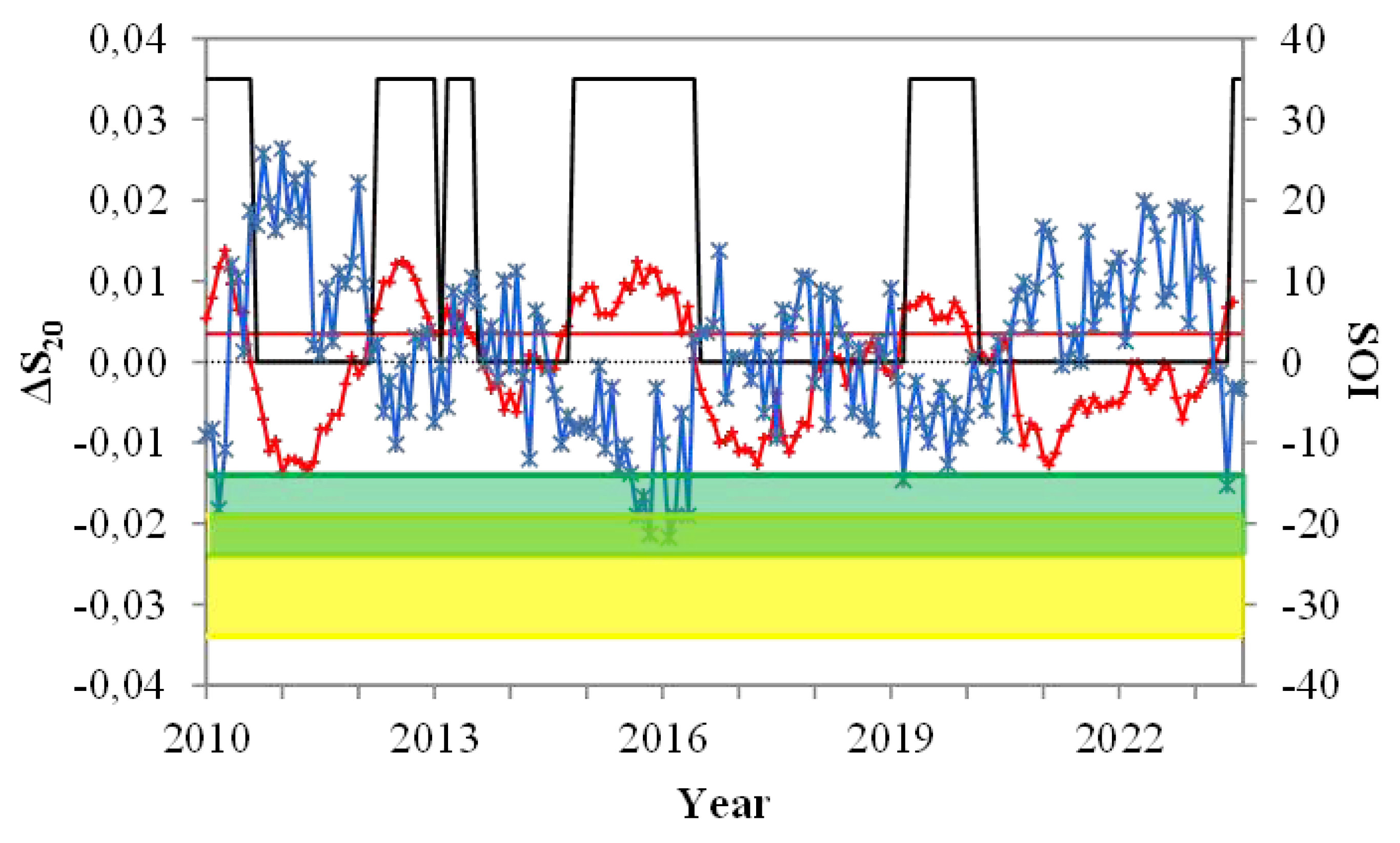
- Forecasting analysis performed by both NTA and M-NTA verified that the 2015-2016 El Niño was characterized as a “moderate to strong” event and not “one of the strongest on record”, as various forecasting reports of that period claimed.
- 2)
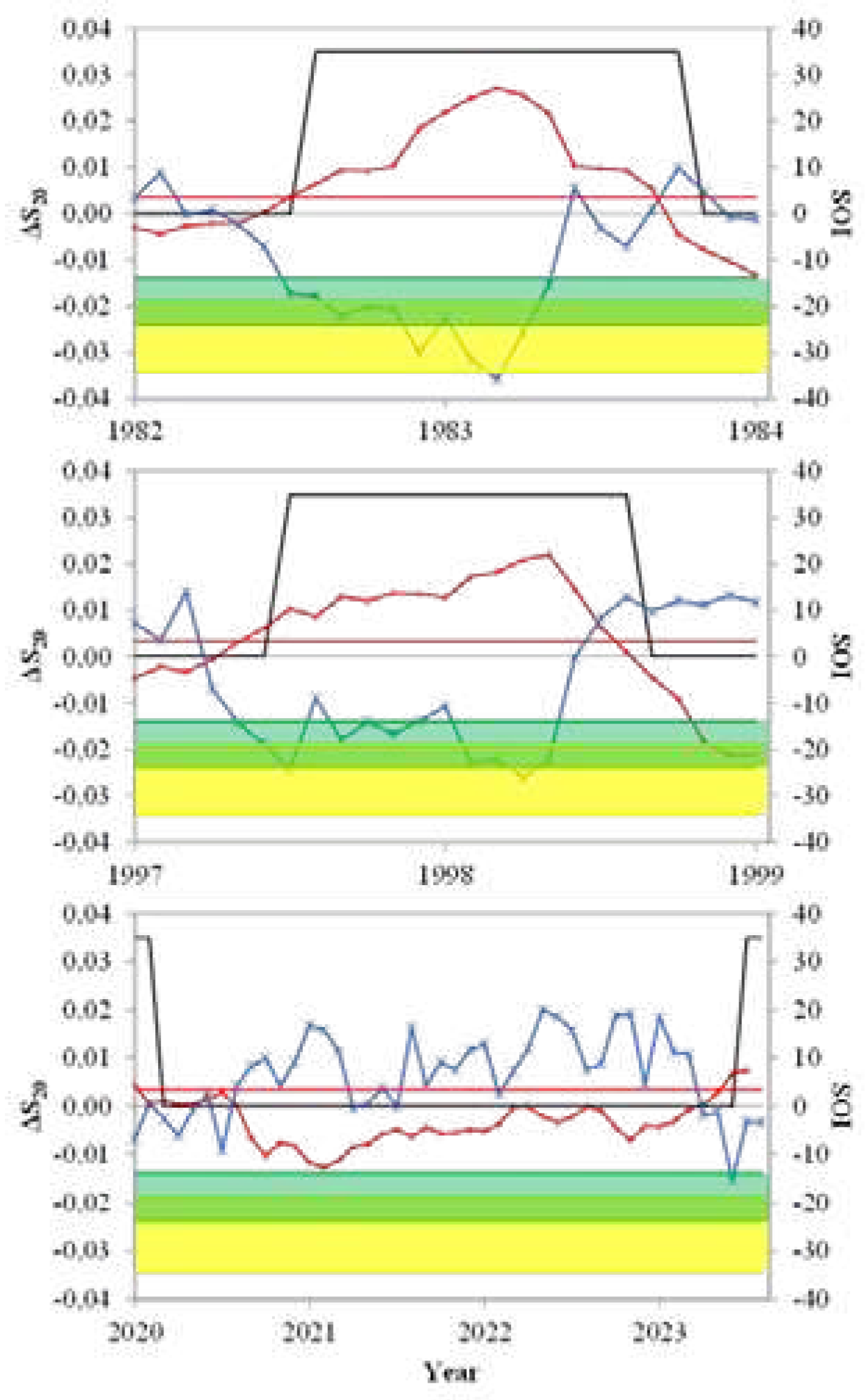
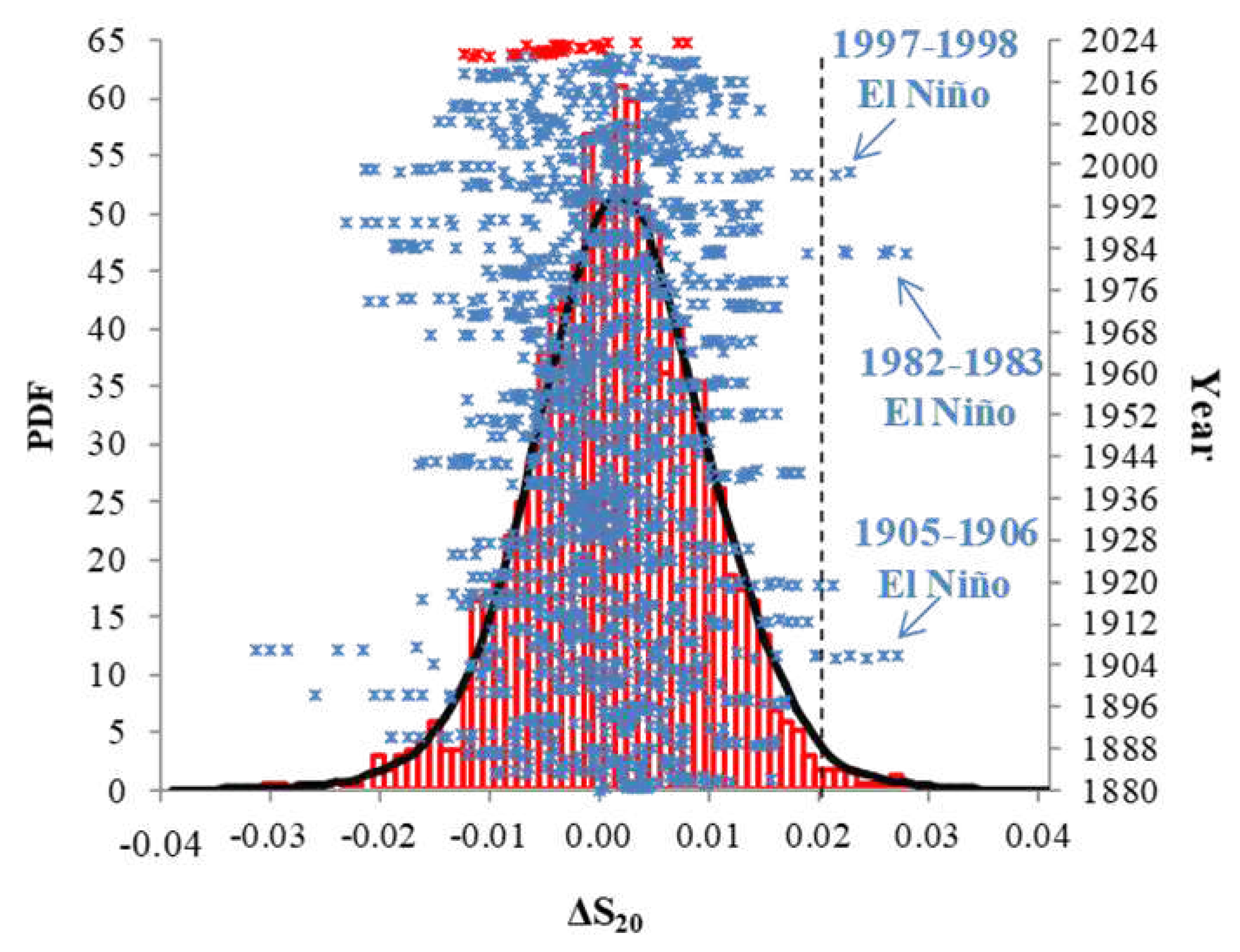
- The SOI time series during the period January 2021 - July 2023 shows a variance that doesn’t foreshadow a strong 2023-2024 El Niño. Furthermore, the variation of entropy change in natural time, during the 2023-2024 El Niño, is less pronounced compared to the corresponding ones during past El Niño events. Finally, according to the probability density function of the ΔS_20 dataset, all the values during January 2021-July 2023 remain below the threshold m + s, where m (s) is the mean (standard deviation) of the dataset.
- 3)
- The M-NTA model appears to adequately estimate the interevent time from 1982 to 1997, two years that correspond to exceptional ONI values of the overall time series. The estimated time of the intermediate event between 1997 and 2016 is estimated to be (17.4, 26.1) years. The average recurrence time of the ONI extremes observed in 2015 was found to be between (18.9, 127.6) years.
- 4)
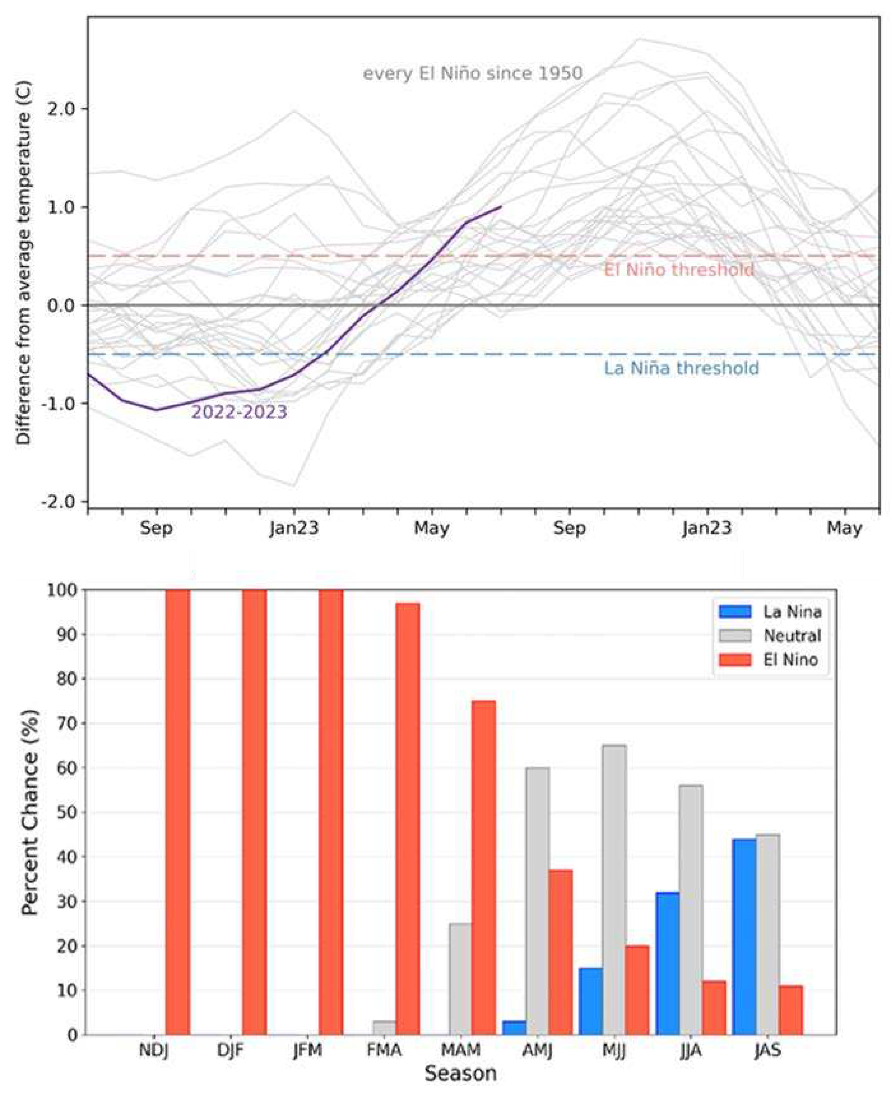
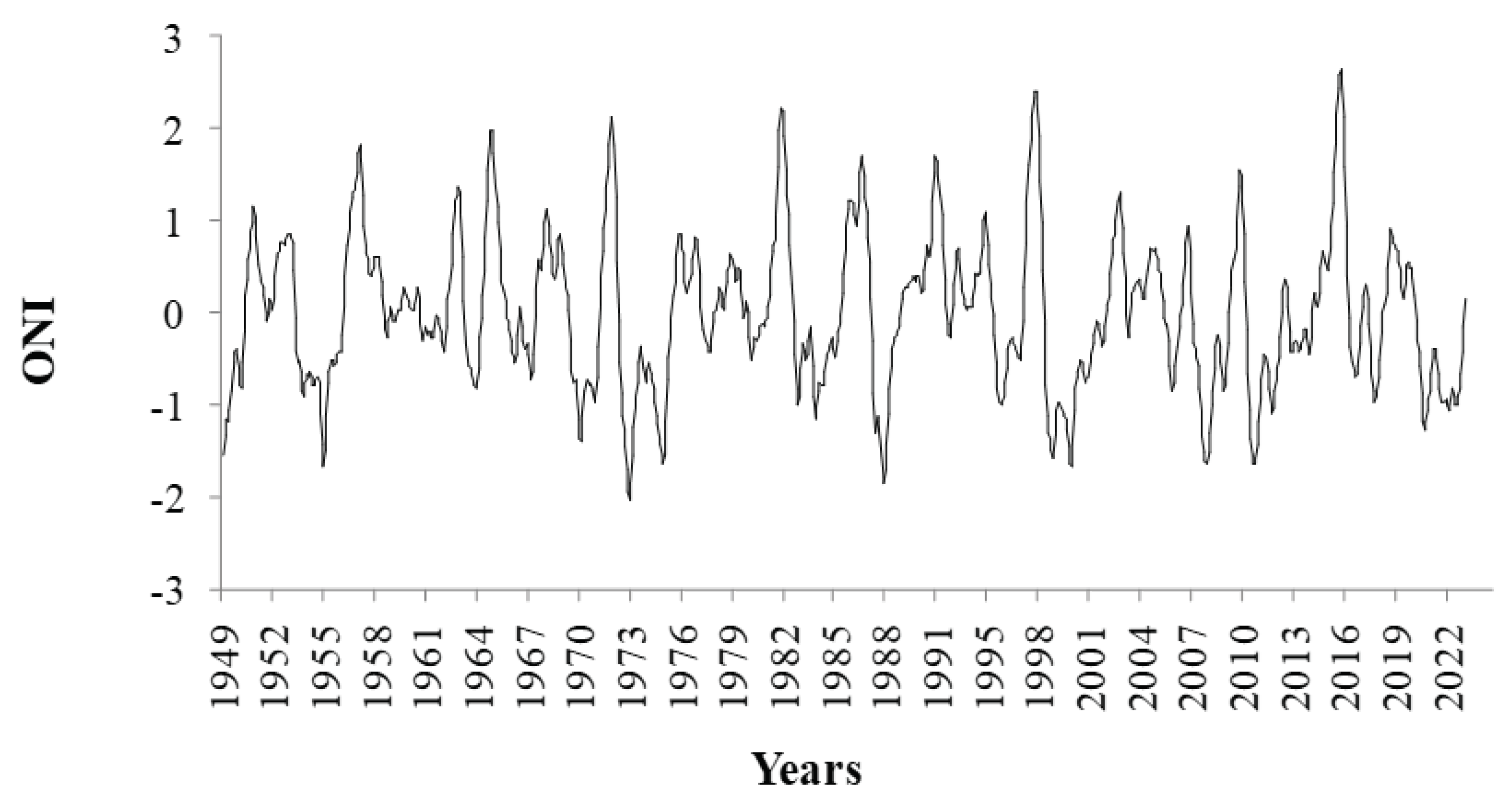
- Regarding the intensity of the ongoing 2023-2024 El Nino event, an ONI value 2.64 occurred only in 2015 (moderate to strong El Nino) and the model predicts a recurrence period of over 85 years. So, it is unlikely to reappear in 2023. Instead, values from 2.14 to 2.40 coming from 1997 or 2016 may appear.
- 5)
- The extremely low SOI values observed in the last three strong ENSO events do not appear to be related to the ongoing ENSO event (2023-2024). On the other hand, the January 1983 SOI value could be related to the 2015-2016 ENSO, while the February 1983 SOI value is expected to affect years after 2038. As for the May 2023 SOI value, it may be related to the minimum SOI of 2019.
Author Contributions
Funding
Data Availability Statement
Conflicts of Interest
References
- Walker, G.T.; Bliss, E.W. World Weather V. Mem. Roy. Meteor. Soc. 1932, 4 (36), 53-84.
- Power, S.B.’ Kociuba, G. The impact of global warming on the Southern Oscillation Index. Clim. Dyn. 2011, 37, 1745–1754. https://link.springer.com/article/10.1007/s00382-010-0951-7.
- Rasmusson, E.M.; Carpenter, T. H. Variations in tropical sea surface temperature and surface wind fields associated with the Southern Oscillation/El Niño. Mon. Weather Rev. 1982, 110(5), 354-384. [CrossRef]
- Troup, A.J. The Southern Oscillation. Q. J. R. Meteorol. Soc. 1965, 91, 490–506. https://rmets.onlinelibrary.wiley.com/doi/abs/10.1002/qj.49709139009.
- Yun, KS., Lee, JY., Timmermann, A. et al. Increasing ENSO–rainfall variability due to changes in future tropical temperature–rainfall relationship. Commun. Earth Environ. 2021, 2, 43. 2021. [CrossRef]
- Neelin, J.D.; Latif, M. El Nino dynamics. Phys. Today 1998, 51(12), 32. [CrossRef]
- Cai, W.; Ng, B.; Geng, T. et al. Anthropogenic impacts on twentieth-century ENSO variability changes. Nat. Rev. Earth Environ. 2023, 4, 407–418. [CrossRef]
- Singh, M.; Sah, S.; Singh, R. The 2023-24 El Niño event and its possible global consequences on food security with emphasis on India. Food Sec. 2023, 15, 1431–1436. [CrossRef]
- Ubilava, D.; Abdolrahimi M. The El Niño impact on maize yields is amplified in lower income teleconnected countries. Environ. Res. Lett., 2019, 14 Article 054008. https://iopscience.iop.org/article/10.1088/1748-9326/ab0cd0/meta.
- Glantz, M.H.; Ramirez, I.J. Reviewing the Oceanic Niño Index (ONI) to Enhance Societal Readiness for El Niño’s Impacts. Int. J. Disaster Risk. Sci., 2020, 11, 394–403. [CrossRef]
- Gurdek-Bas, R.; Benthuysen, J.A.; Harrison, H.B. et al.: The El Niño Southern Oscillation drives multidirectional inter-reef larval connectivity in the Great Barrier Reef. Sci. Rep. 2022,12, 21290. [CrossRef]
- Khanke, H. R.; Azizi, M.; Asadipour, E.; Barati, M. Climate Changes and Vector-borne Diseases with an Emphasis on Parasitic Diseases: A Narrative Review. Health Emerg. Disasters Quart., 2023 8(4), 293-300. [CrossRef]
- Thompson A. El Niño May Break a Record and Reshape Weather around the Globe. Scientific American, 2023, https://www.scientificamerican.com/article/el-nino-may-break-a-record-and-reshape-weather-around-the-globe/.
- Yin, J.; Xu, J.; Xue, Y.; Xu, B.; Zhang, C.; Li, Y.; Ren, Y. Evaluating the impacts of El Niño events on a marine bay ecosystem based on selected ecological network indicators. Sci. Total Environ., 2021, 763, 144205. [CrossRef]
- Barber, R.T.; Chavez, F.P. Biological consequences of El Nino. Science. 1983, 222(4629), 1203-1210. https://www.science.org/doi/abs/10.1126/science.222.4629.1203.
- WMO: 2022, https://public.wmo.int/en/our-mandate/climate/el-ni%C3%B1ola-ni%C3%B1a-update.
- Hamlington, B. D.; Willis, J. K.; Vinogradova, N. The emerging golden age of satellite altimetry to prepare humanity for rising seas. Earth's Future, 2023, 11(11), e2023EF003673. [CrossRef]
- Omid, A. Advances and challenges in climate modeling. Climatic Change, 2022, 170(1-2). [CrossRef]
- Varotsos, C.A.; Tzanis, C.G.; Sarlis, N.V. On the progress of the 2015–2016 El Niño event. Atmos. Chem. Phys., 2016a, 16, 2007–2011. [CrossRef]
- Varotsos, C.A.; Tzanis, C.; Cracknell, A.P. Precursory signals of the major El Niño Southern Oscillation events. Theor. Appl. Climatol., 2016b, 124(3), 903-912. https://link.springer.com/article/10.1007/s00704-015-1464-4.
- National Oceanic and Atmospheric Administration (NOAA), El Niño/Southern Oscillation (ENSO) Diagnostic Discussion, issued by Climate Prediction Center. 2023, https://www.cpc.ncep.noaa.gov/products/analysis_monitoring/enso_advisory/ensodisc.shtml.
- Varotsos, P. A.; Sarlis, N.V.; Skordas, E.S. Long-range correlations in the electric signals that precede rupture. Phys. Rev. E, 2002, 66, 011902. https://journals.aps.org/pre/abstract/10.1103/PhysRevE.66.011902.
- Varotsos, P. A.; Sarlis, N.V.; Tanaka, H.K.; Skordas, E.S. Some properties of the entropy in the natural time. Phys. Rev. E, 2005, 71, 032102. [CrossRef]
- Sarlis, N.V.; Skordas, E.S.; Varotsos, P.A. Nonextensivity and natural time: The case of seismicity. Phys. Rev. E, 2010 82, 021110. https://journals.aps.org/pre/abstract/10.1103/PhysRevE.82.021110..
- Sarlis, N.V.; Skordas, E.S.; Varotsos, P.A. Similarity of fluctuations in systems exhibiting Self-Organized Criticality, EPL 2011a ,96, 28006. [CrossRef]
- Sarlis, N.V.; Skordas, E.S.; Varotsos, P.A. The change of the entropy in natural time under time-reversal in the Olami– Feder–Christensen earthquake model. Tectonophysics, 2011b, 513, 49– 53. [CrossRef]
- Varotsos, P.A.; Sarlis, N.V.; Skordas, E.S. Natural Time Analysis: The new view of time. Precursory Seismic Electric Signals, Earthquakes and other Complex Time-Series. Springer-Verlag, Berlin Heidelberg. ISBN 978-3-642-16449-4. 2011. [CrossRef]
- Fawcett, T. An introduction to ROC analysis. Pattern Recogn. Lett., 2006, 27, 861–874. [CrossRef]
- Sarlis, N.V.; Christopoulos, S.-R.G. Visualization of the significance of Receiver Operating Characteristics based on confidence ellipses. Comput. Phys. Commun., 2014 185, 1172–1176. [CrossRef]
- Varotsos, C.A.; Efstathiou, M.N.; Christodoulakis, J. The lesson learned from the unprecedented ozone hole in the Arctic in 2020 A novel nowcasting tool for such extreme event. J. Atmos. Sol.-Terr. Phys., 2020a, 207, 105330. [CrossRef]
- Varotsos C.A.; Mazei Y.; Novenko E.; Tsyganov A.N.; Olchev A.; Pampura T.; Mazei N.; Fatynina Y.; Saldaev D.; Efstathiou M.A. New Climate Nowcasting Tool Based on Paleoclimatic Data. Sustainability, 2020b, 12, 5546. [CrossRef]
- Varotsos, C.A.; Mazei, Y.; Saldaev, D.; Novenko, E.; Efstathiou, M.; Voronova, T.; Xue, Y. Nowcasting of air pollution episodes in megacities: A case study for Athens, Greece. Atmos. Pollut. Res., 2021, 12, 101099. [CrossRef]
- Varotsos P.A.; Sarlis N.V.; Skordas E.S. Order parameter fluctuations in natural time and b-value variation before large earthquakes. Nat. Hazards Earth Syst. Sci., 2012, 12(11), 3473-3481. [CrossRef]
- Varotsos P.A.; Sarlis N.V.; Skordas E.S.; Tanaka H. A plausible explanation of the b-value in the Gutenberg-Richter law from first Principles. Proc. Jpn. Acad., Ser. B, 2004,80(9), 429-434. https://www.jstage.jst.go.jp/article/pjab/80/9/80_9_429/_article/-char/ja/.
| ONI value x0 |
Nowcasted mean inter-event time t [in years] |
The lower limit of the 95%-confidence interval of t. |
The upper limit of the 95%-confidence interval of t. |
|---|---|---|---|
| 1.74 | 3.0 (2.6) | 2.5 (2.2) | 3.7 (3.2) |
| 1.84 | 3.5 (3.1) | 2.9 (2.6) | 4.3(3.8) |
| 1.94 | 4.1 (3.6) | 3.4 (3.1) | 5.1 (4.4) |
| 2.04 | 4.8 (4.3) | 4.0 (3.6) | 6.0 (5.2) |
| 2.14 | 9.2 (8.2) | 7.6 (6.9) | 11.4 (10.0) |
| 2.24 | 12.1 (10.8) | 10.1 (9.2) | 15.1 (13.2) |
| 2.57 | 51.4 (45.9) | 42.8 (38.9) | 64.3 (56.0) |
| 2.64 | 102.1 (91.2) | 85.1 (77.3) | 127.6 (111.1) |
| SOI value x0 |
Nowcasted mean inter-event time t [in years] |
The lower limit of the 95%-confidence interval of t |
The upper limit of the 95%-confidence interval of t |
|---|---|---|---|
| -19.0 | 3.6 | 3.0 | 4.5 |
| -21.3 | 5.4 | 4.5 | 6.8 |
| -21.7 | 5.8 | 4.9 | 7.2 |
| -26.1 | 12.5 | 10.4 | 15.6 |
| -30.0 | 24.6 | 20.6 | 30.6 |
| -31.4 | 31.4 | 26.2 | 39.1 |
| -35.7 | 66.3 | 55.4 | 82.5 |
Disclaimer/Publisher’s Note: The statements, opinions and data contained in all publications are solely those of the individual author(s) and contributor(s) and not of MDPI and/or the editor(s). MDPI and/or the editor(s) disclaim responsibility for any injury to people or property resulting from any ideas, methods, instructions or products referred to in the content. |
© 2024 by the authors. Licensee MDPI, Basel, Switzerland. This article is an open access article distributed under the terms and conditions of the Creative Commons Attribution (CC BY) license (http://creativecommons.org/licenses/by/4.0/).


