Dynamic Comprehensive Evaluation of a 660MW Ultra-Supercritical Coal-Fired Unit Based on Improved Criteria Importance through Inter-criteria Correlation and Entropy Weight Method

Preprint

Article

Dynamic Comprehensive Evaluation of a 660MW Ultra-Supercritical Coal-Fired Unit Based on Improved Criteria Importance through Inter-criteria Correlation and Entropy Weight Method

Altmetrics

Downloads

Views

Comments

A peer-reviewed article of this preprint also exists.

Haotian Yuan,

Xiaojing Ma^*,

Zening Cheng,Tusongjiang Kari

Haotian Yuan,

Xiaojing Ma^*,

Zening Cheng,Tusongjiang Kari

This version is not peer-reviewed

Submitted:

05 February 2024

Posted:

06 February 2024

You are already at the latest version

Alerts

Abstract

To address the issue of traditional static evaluation models being unable to comprehensively analyse the performance of ultra-supercritical coal-fired units under varying loads, we propose a dynamic comprehensive evaluation model based on the improved Criteria Importance Through Inter-criteria Correlation (CRITIC) method and Entropy Weight Method (EWM). The comprehensive performance evaluation index system of ultra-supercritical coal fired units is constructed by examining the boiler performance, turbine performance, plant power performance, environmental performance, and flexible performance of coal powered units. The CRITIC and EWM methods are used to calculate the weights of the indicators, which are then combined with the static evaluation results. Using a dynamic comprehensive evaluation model, we analysed ultra-supercritical coal-fired units, taking into account time weight. This allowed us to obtain the comprehensive dynamic real-time evaluation value of the units under different loads. The research indicates that the dynamic comprehensive evaluation model, which uses an improved CRITIC and EWM, has significant advantages in improving evaluation accuracy, weight-balanced distribution, and generality. Provides more accurate, reasonable, and reliable evaluation results for practical decision making.

Keywords:

Subject: Engineering - Energy and Fuel Technology

1. Introduction

As global climate change and pollution continue to worsen, countries have set carbon-neutral and dual-carbon targets to drive the transformation of the energy industry towards a more sustainable direction [1]. As an important part of traditional energy, the development and reform of coal-fired units under the background of dual carbon is particularly important [2]. In recent years, with increasing environmental concerns and the rise of clean energy, the comprehensive assessment of coal-fired units has become increasingly important [3]. In recent years, the comprehensive performance evaluation methods of coal-fired power plants have emerged, and many scholars at home and abroad have proposed a variety of comprehensive evaluation methods, such as analytical hierarchy process, entropy weight method, rank-sum ratio comprehensive evaluation method and fuzzy comprehensive evaluation method [4]. Ma et al. [5] proposed a comprehensive dynamic performance evaluation method to comprehensively understand the overall performance of coal-fired units under load changes, and to provide a basis for future optimization and improvement. Chen et al. [6] used fuzzy analytical hierarchy process and improved criteria importance through intercriteria correlation (CRITIC) to empower evaluation indicators, which reflected the rationality of comprehensive evaluation indicators and the effectiveness of evaluation methods. Wang et al. [7] determined the weights of the evaluation indicators by combining the entropy weighting method (EWM) and the subjective weighting method to achieve a comprehensive evaluation of the flexibility of coal-fired units. Huang et al. [8] analysed the distribution characteristics of carbon emissions from buildings across six aspects and provided recommendations for development. Wang et al. [9] assessed the long-term operational status of near-zero emission coal-fired units. Ma et al. [10] established the assessment framework of source-network-load interaction to provide a set of systematic indicators and methods for low-carbon development of coal-fired units and a more sustainable development path for coal-fired power plants. Comprehensive evaluation can be divided into static comprehensive evaluation and dynamic comprehensive evaluation [11]. In the static comprehensive evaluation, the evaluation object is evaluated comprehensively in a single period based on the information of each index of the evaluation object [11]. Dynamic comprehensive evaluation uses the same evaluation method to perform static comprehensive evaluation of evaluation objects at different time periods, and integrates with information aggregation operators to obtain the dynamic comprehensive evaluation value of evaluation objects [12]. At present, many scholars are paying attention to dynamic comprehensive evaluation. In 2007, Guo et al. [13] first proposed two types of information aggregation operators that can be used for dynamic comprehensive evaluation. On this basis, Li et al. [14] proposed a series of dynamic comprehensive evaluation methods based on the technique for order preference by similarity to ideal solution. Wang et al. [15] built an evaluation index system of the basic emergency response capability of the power grid based on the analysis of time and space dimensions, in order to achieve a dynamic and comprehensive evaluation of the emergency response capability of the power grid. Zhang et al. [16] proposed a new dynamic comprehensive evaluation model of multi-source uncertainty indicators based on the generalised grey incentive factors, and proved the effectiveness and feasibility of the model in combination with practical cases. This paper aims to solve the problem that the traditional static evaluation model cannot analyze the comprehensive performance of ultra-supercritical coal-fired units under varying loads. The evaluation index system for ultra-supercritical coal-fired units was constructed using the entropy weight method and the improved CRITIC method to determine the static weights of each index. A dynamic comprehensive evaluation model was then created by combining the time-series three-dimensional data table. On the basis of ensuring the accuracy, reliability and rationality of the evaluation results, the key indicators affecting the performance of coal-fired units are explored.

2. The Construction of Index System

2.1. Principle of Index System Construction

Coal-fired units are an extremely complex energy consumption system, combined with the economic and environmental benefits of the development of coal-fired units, the index system includes all aspects of the characteristics of the development of coal-fired units under the dual-carbon target, and can reflect the development characteristics of coal-fired units under the low-carbon target. Therefore, the index system should be based on the following construction principles [17]:

The principle of independence: the degree of coupling between the primary index and the secondary index of the index system should be chosen to be low, and redundancy, cross-information and noise between indicators should be reduced.

Operability principle: the selection of indicators should be easy to quantify, the data source should be reliable and easy to measure, collect and obtain, and it should ensure that the indicator data can be processed in a standardised way.

Completeness principle: the selection of evaluation indicators should be able to reflect the characteristics and connotation of the overall performance of coal-fired units in a comprehensive, multifaceted and accurate manner. When selecting evaluation indicators, special attention should be paid to the selection of qualitative and quantitative indicators.

Objectivity principle: in the selection of indicators, the selected indicators can truly and accurately reflect the objectivity of the evaluation object, without complicating subjective factors, so as to make a fair and impartial comprehensive evaluation of the evaluation object.

Dynamic principle: the index system is a dynamically changing process in the selection process. Therefore, the dynamic change of indicators over time should be fully considered in the selection of indicators. Horizontal comparison indicators should be selected with a clear trend of change in order to differentiate, so as to avoid the selection of no change or small changes in the data.

2.2. Index System of Coal-Fired Units

The evaluation criteria for coal-fired units are based on current national standards, relevant industry regulations, current management standards and methods of various Group companies, and local processes [18]. According to the selection principle of the evaluation index system, through the feasibility analysis of the initial index, combined with the actual situation of the site, the main factors of the coal-fired power plant are decomposed layer by layer, and the evaluation index system of the comprehensive performance of the coal-fired power plant is constructed, including 5 first-level evaluation indicators and 23 second-level evaluation indicators. Figure 1 shows the comprehensive evaluation index system of coal-fired units.

Materials and Methods should be described with sufficient details to allow others to replicate and build on published results. Please note that publication of your manuscript implicates that you must make all materials, data, computer code, and protocols associated with the publication available to readers. Please disclose at the submission stage any restrictions on the availability of materials or information. New methods and protocols should be described in detail while well-established methods can be briefly described and appropriately cited.

Research manuscripts reporting large datasets that are deposited in a publicly avail-able database should specify where the data have been deposited and provide the relevant accession numbers. If the accession numbers have not yet been obtained at the time of submission, please state that they will be provided during review. They must be provided prior to publication.

Interventionary studies involving animals or humans, and other studies require ethical approval must list the authority that provided approval and the corresponding ethical approval code.

This is an example of a quote.

3. Methods

3.1. Improve CRITIC Method

Criteria Importance Through Intercrieria Correlation (CRITIC) [6] is an objective weighting method based on data volatility, and considers the comparative strength of evaluation indicators and the principle of conflict to comprehensively measure the objective weights between indicators.

To address issues with determining evaluation index weights in the original CRITIC, this paper introduces the concept of information entropy to improve the method, resulting in ICRITIC. The original CRITIC method has problems in calculating indicator weights, mainly due to the excessive weight of indicators caused by direct attribute assignment and correlation between indicators. This issue affects the accuracy and fairness of evaluation results.

ICRITIC is highly objective and versatile, allowing for a comprehensive reflection of the relationship between evaluation indicators. It also avoids any potential bias towards certain indicators that may be present in other methods. In practical applications, the ICRITIC method proposed in this paper provides a more accurate, reasonable, and reliable way to determine the weight of evaluation indicators.

Step 1: select m evaluation indications for n evaluation objects, establish the evaluation indicator system, construct the level matrix and standardize the processing.

Step 2: the variability of the evaluation index

\{\begin{matrix} {\bar{x}}_{j} = \frac{1}{m} \sum_{i = 1}^{m} x_{i j} \\ S_{j} = \sqrt{\frac{\sum_{i = 1}^{m} {(x_{i j} - {\bar{x}}_{j})}^{2}}{m - 1}} \end{matrix}, (1 \leq i \leq m, 1 \leq j \leq n),

(1)

In the formula,

x_{i j}

is the evaluation matrix of each index,

S_{j}

is the standard deviation of the evaluation index.

Step 3: the conflict of evaluation indicators

R_{j} = \sum_{i = 1}^{m} (1 - |r_{i j}|), (1 \leq i \leq m, 1 \leq j \leq n)

(2)

In the formula,

R_{j}

is the conflict of evaluation index.

Step 4: information of evaluation indicators

\{\begin{matrix} p_{i j} = \frac{{x^{'}}_{i j}}{\sum_{j = 1}^{n} {x^{'}}_{i j}} \\ E_{j} = - \frac{1}{ln m} \sum_{i = 1}^{m} p_{i j} ln p_{i j} \\ C_{j} = (E_{j} + \frac{S_{j}}{{\bar{x}}_{j}}) \times R_{j} \end{matrix}, (1 \leq i \leq m, 1 \leq j \leq n),

(3)

In the formula,

p_{i j}

is the characteristic of evaluation index,

E_{j}

is the information entropy of evaluation index,

C_{j}

is the information content of evaluation index.

Step 5: objective weights of evaluation indicators

w_{j}^{'} = \frac{C_{j}}{\sum_{j = 1}^{n} C_{j}}, (1 \leq j \leq n)

(4)

In the formula,

w_{j}^{'}

is the weight of evaluation index.

3.2. Entropy Weight Method

Entropy weight method (EWM) [18,19] is an objective weighting method. The weight of each index’s entropy is calculated based on its dispersion, and the weight of the objective index is then determined.

Step 1: The original data matrix composed of m evaluation objects and n evaluation indicators is denoted as

X = {(x_{i j})}_{m \times n}

Step 2: data normalization processing

\{\begin{matrix} {x^{'}}_{i j} = \frac{x_{i j} - min (x_{i j})}{max (x_{i j}) - min (x_{i j})} \\ {x^{'}}_{i j} = \frac{max (x_{i j}) - x_{i j}}{max (x_{i j}) - min (x_{i j})} \end{matrix}, (1 \leq i \leq m, 1 \leq j \leq n),

(5)

In the formula,

x_{i j}^{'}

is the standardised value of the evaluation indicators (without negative indicators).

Step 3: characteristic proportion of evaluation index

f_{i j} = {x^{'}}_{i j} / \sum_{j = 1}^{n} {x^{'}}_{i j}, (1 \leq i \leq m, 1 \leq j \leq n)

(6)

In the formula,

f_{i j}

is the characteristic of evaluation index.

Step 4: the information entropy of evaluation index

H_{j} = - \frac{1}{ln m} \sum_{i = 1}^{m} f_{i j} ln f_{i j}, (1 \leq i \leq m, 1 \leq j \leq n)

(7)

In the formula,

H_{j}

is the information entropy of evaluation index.

Step 5: objective weights of evaluation indicators

w_{j} = \frac{1 - H_{j}}{\sum_{j = 1}^{n} (1 - H_{j})},, (1 \leq j \leq n)

(8)

In the formula,

w_{j}

is the weight of evaluation index.

3.3. Combinatorial Weighting

In order to avoid an accident in the calculation process and the neglect of indicators by objective assignment, the overall weight is as close as possible to the objective weight, taking into account the advantages of each objective weight assignment. This paper adopts the minimum information entropy principle to synthesize the index weights obtained by ICRITIC and EWM. The Lagrange multiplier method is then used to optimize and obtain the comprehensive weights [20,21].

{W_{j}}^{C W} = \frac{\sqrt{W_{j}^{C R I T I C} * W_{j}^{E W M}}}{\sum_{j = 1}^{n} \sqrt{W_{j}^{C R I T I C} * W_{j}^{E W M}}}

(9)

In the formula,

{W_{j}}^{C W}

is the combined weight of the evaluation index,

W_{j}^{C R I T I C}

is the weight of the evaluation index calculated by CRITIC,

W_{j}^{E W M}

is the weight of the evaluation index calculated by EWM.

3.4. Aggregation Operator

In 1998, Yager proposed the ordered weighted average (OWA) operator [22,23], which is an aggregation method of multi-attribute decision information between the maximum and minimum operators. Later, Guo et al. [13] proposed time ordered weighted averaging (TOWA) operator and time ordered weighted geometric averaging (TOWGA) operator.

3.4.1. TOWA Operator

Let

N = \{1, 2, \dots, n\}

〈u_{i}, a_{i}〉

is TOWA pair, where

u_{i}

is the time-induced component and

a_{i}

is the data component.

F (〈u_{1}, a_{1}〉, \dots, 〈u_{p}, a_{p}〉) = \sum_{j = 1}^{p} λ_{j} b_{j}

(10)

In the formula, vectors

λ = {(λ_{1}, λ_{2}, \dots, λ_{p})}^{T}

and vectors

\vec{F}

are related weighted vectors,

λ_{j} \in [0, 1]

and

\sum_{j = 1}^{n} λ_{j} = 1

b_{j}

represents the second component of the TOWA operator corresponding to time j, so the function is called an n-dimensional TOWA operator.

3.4.2. TOWGA Operator

Let

N = \{1, 2, \dots, n\}

〈v_{i}, c_{i}〉

is TOWA pair, where

v_{i}

is the time-induced component and

c_{i}

is the data component.

G (〈v_{1}, c_{1}〉, \dots, 〈v_{p}, c_{p}〉) = \prod_{j = 1}^{p} d_{j}^{{λ^{'}}_{j}}

(11)

In the formula, vectors

λ^{'} = {({λ^{'}}_{1}, {λ^{'}}_{2}, \dots, {λ^{'}}_{p})}^{T}

and vectors

\vec{G}

are related weighted vectors,

λ_{j}^{'} \in [0, 1]

and

\sum_{j = 1}^{n} {λ^{'}}_{j} = 1

d_{j}

represents the second component of the TOWA operator corresponding to time j, so the function is called an n-dimensional TOWA operator.

3.4.3. TOWA-TOWGA Hybrid Model

According to the definition of aggregation operators, TOWA operators care about functionality and TOWGA operators care about balance, both have advantages and disadvantages [24]. Therefore, based on the static evaluation results and considering the influence of the time factor, the TOWA-TOWGA hybrid model is used to perform a dynamic comprehensive evaluation of the performance of ultra-supercritical coal-fired units.

Y_{i} = α_{1} F (λ_{t}) + α_{2} G (λ_{t})

(12)

In the formula,

α_{1}

and

α_{2}

are the proportion of TOWA and TOWGA operators respectively,

0 \leq α_{1} \leq 1

0 \leq α_{2} \leq 1

α_{1} + α_{2} = 1

3.5. Determination of Time Weight

In dynamic comprehensive evaluation, time weighting reflects the relative importance of the evaluation object in different time periods in the process of information aggregation. Therefore, both subjective and objective factors need to be fully considered when determining time weights. On the one hand, the knowledge and experts experience should be taken into account, and on the other hand, objective information from time samples should be taken into account [13]. For the solution of the time weight, it is necessary to have a definition of the "time degree":

θ = \sum_{t = 1}^{p} \frac{p - t}{p - 1} λ_{t}

(13)

In the formula,

θ

is the time degree,

λ_{t}

is the time weight vector.

Table 1 shows the value of "time degree" reflects the importance of time series to operators in the process of aggregation. When

θ

approaches 0, it indicates that the decision maker is paying more attention to the data in the most recent period. When

θ

approaches 1, it indicates that the decision maker pays more attention to data in the distant time period. When

θ

is the tent threshold with a value of 0.5, it indicates that the decision maker attaches the same importance to the sample information in each time period.

Under the condition of determining the "time degree", the programming method is used to determine the time weight. Through in-depth mining of sample information and comprehensive consideration of the relative importance of the evaluation object in different time periods, the time weight vector of the sample is clarified. Calculate the weight coefficient according to the variance formula [13]:

D^{2} (λ) = \sum_{i = 1}^{p} \frac{1}{p} {[λ_{t} - E (λ)]}^{2} = \frac{1}{p} \sum_{i = 1}^{p} λ_{t}^{2} - \frac{1}{p^{2}}

(14)

In the formula,

D^{2} (λ)

is the variance,

E (λ)

is the mean value of the time weight coefficient. TTherefore, the least variance method is used to solve the nonlinear programming problem [13]:

\{\begin{matrix} min (\frac{1}{p} \sum_{i = 1}^{p} λ_{t}^{2} - \frac{1}{p^{2}}) \\ s t . \{\begin{matrix} θ = \sum_{= 1}^{n} \frac{p - t}{p - 1} λ_{t} \\ \sum_{t = 1}^{p} λ_{t} = 1 \end{matrix} \\ λ_{t} \in [0, 1] \\ t = 1, 2, \dots, n \end{matrix}

(15)

4. Results and discussion

Based on the consultation of experts and the combination of the actual situation of the site, this paper takes the operating data of a 660MW coal-fired unit in Xinjiang from February 2023 to August 2023 as the research object. The operating data with a stable operating time of more than 1 hour and a load variation range within ±2% have been selected for the analysis. At the same time, the variable working condition data with load variation range between 25% and 98%, excluding the selected stable operation data, is analysed based on the three sets of data selected in this paper. Due to the influence of environmental factors in the summer, turbine heat acceptance (THA) does not operate at 100% heat consumption during operation. Therefore, this paper selects data from summer 90%THA coal-fired units for comparative analysis.

4.1. Determination of Combinatorial Weights

The combined weights of evaluation indicators were obtained based on the objective weight data obtained by ICRITIC and EWM. Table 2 and Table 3 respectively show the combined weights of different evaluation indicators for the coal-fired units in different environments, where

T_{1}

T_{6}

represent February, March, April, June, July and August respectively.

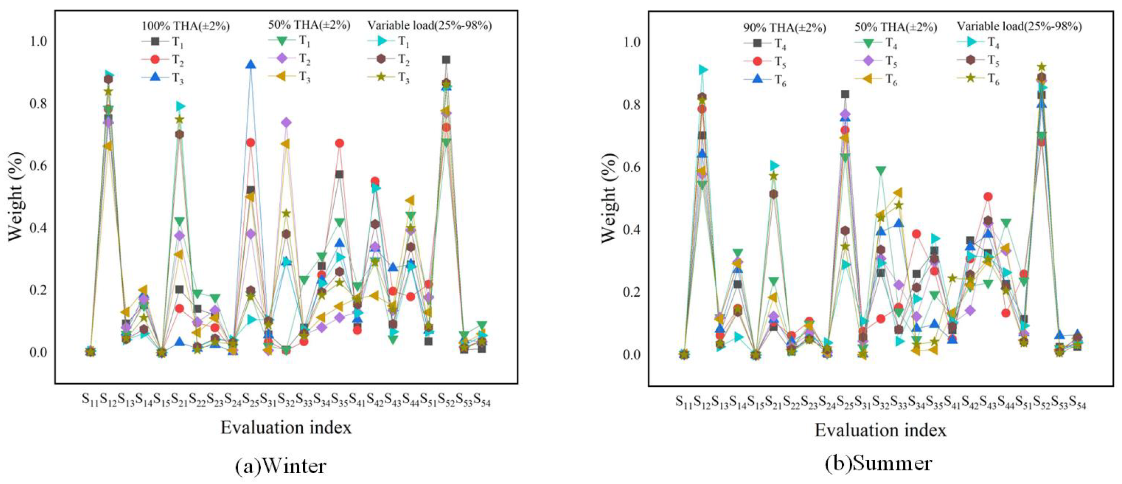
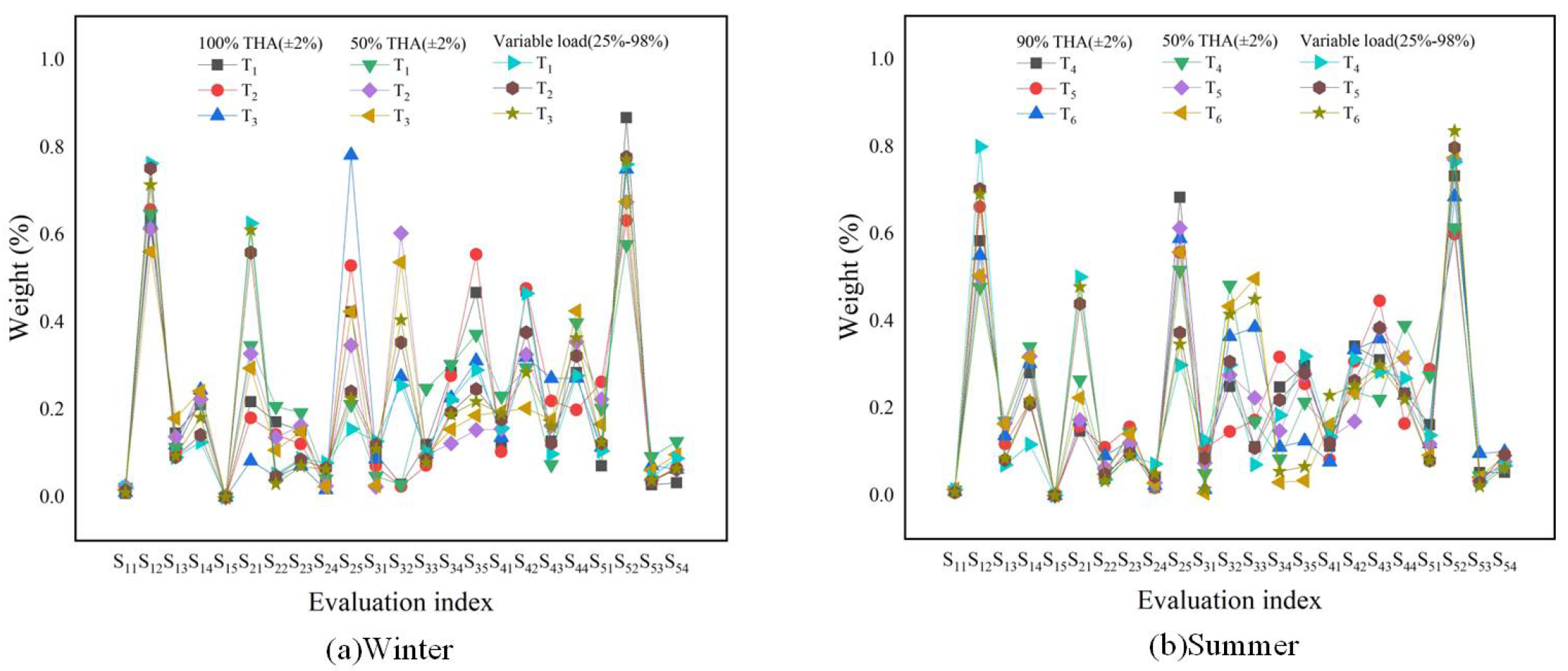
According to Figure 2 and Figure 3, to evaluate the effectiveness of ICRITIC, we tested and calculated the weight of evaluation indicators and compared it with CRITIC before the improvement. The comparison results indicate that the improved ICRITIC can eliminate any unjustified weight bias present in the original method. This leads to a more accurate evaluation of index weight and a more objective and comprehensive assessment.

4.2. Determination of Combinatorial Weights

According to the advice of relevant experts, when

θ

is the tent threshold with a value of 0.3 and solve the programming equation with minimum variance to obtain the time weight vector:

λ = [\begin{matrix} 0 . 1333 & 0 . 3333 & 0 . 5333 \end{matrix}]

The static assessment results of each index are aggregated over time to produce the dynamic comprehensive assessment of the index. Where

α_{1}

and

α_{2}

are the tent threshold with a value of 0.5. Tab. 4 shows the final evaluation results of each indicator.

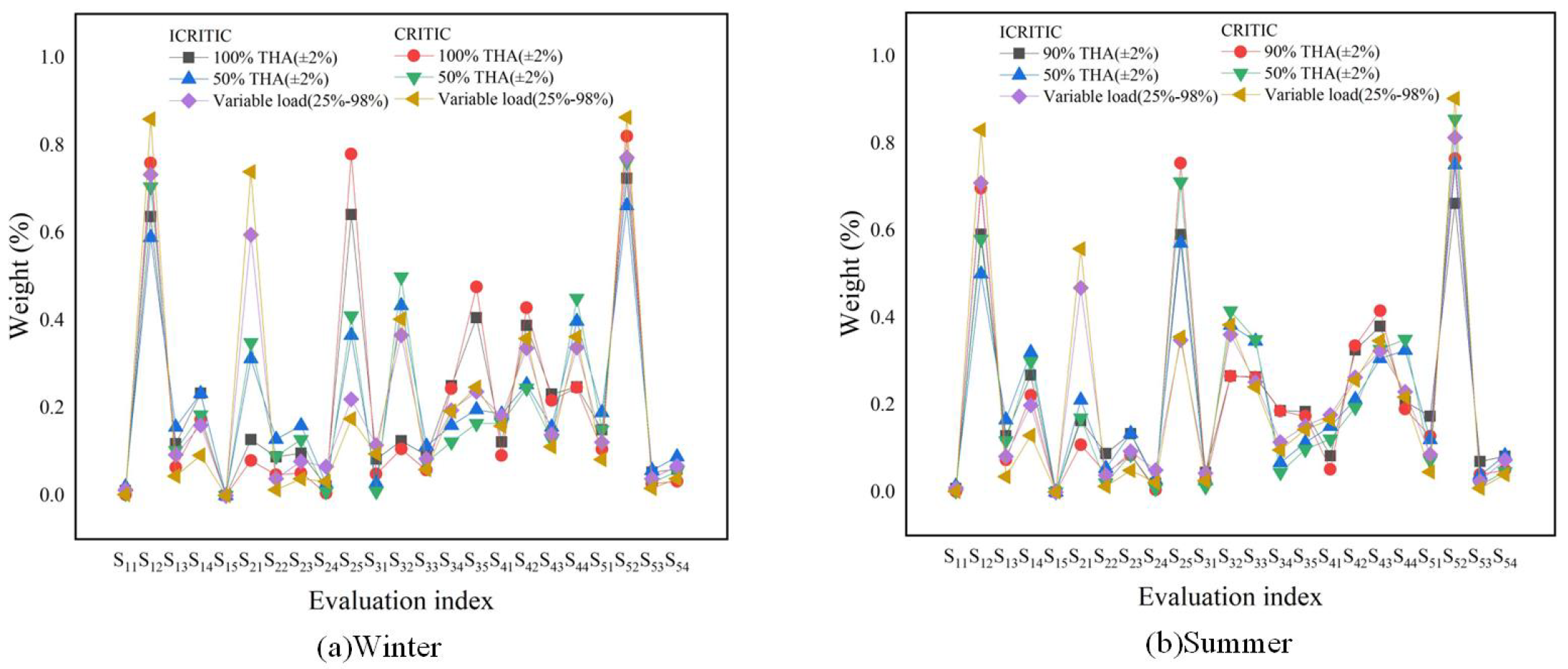
According to Table 4 and Figure 4, analysis of evaluation results under different circumstances:

From the boiler performance, the load of coal-fired units fluctuates greatly in summer and winter, and the load change can lead to the adjustment of system parameters that affect the performance of boiler oxygen and the air preheater. The temperature difference between summer and winter is large, causing the air heater to be affected by the temperature change and thus affecting the air leakage rate of the air heater.

From the steam turbine performance, under different operating conditions in summer and winter, coal-fired units need to adjust the running state of the steam turbines to meet the needs of the power grid. The main steam pressure increases in weight while the condenser temperature decreases slightly due to load variation. The change in load will result in a change in steam properties which will have an effect on the operating condition of the condenser. In summer, when the ambient temperature is higher, the temperature of the cooling water may rise, causing the temperature of the condenser to increase. Although the ambient temperature is lower in winter, the temperature of the cooling water can still be higher.

From the power consumption rate performance, under varying operating conditions in different seasons, the circulating pump may require the use of valves or frequency conversion speed regulation to adjust the flow rate. This can cause the operating point of the circulating pump to deviate from the design condition, resulting in decreased pump efficiency. These factors can lead to an increase in power consumption of the circulating pump. During winter operation at 100% THA (±2%), the amount of coal burned increases, resulting in a corresponding increase in SO₂ emissions from flue gas. To comply with stringent environmental emission standards, the quantity of desulfurizer will be increased, resulting in higher power consumption of the desulfurization system.

From the environmental performance, the combustion system experiences varying load conditions during summer and winter operations, which can result in combustion process instability. The desulfurization system’s performance has been reduced, and the flue gas is now contaminated with incompletely combusted pulverized coal and particulate matter. This results in an increase in SO₂ concentration, which in turn leads to higher rates of ammonia escape and smoke emissions.

From the flexibility performance, the coal-fired units will adjust their load instantly based on the power system’s demand during different load operations in summer and winter. Automatic generation control (AGC) must respond quickly to these changes to ensure the frequency stability of the frequency of the power system, so as to meet the requirements of the power system and ensure the quality and reliability of the power supply.

According to the comparison of the improved critic, it can be seen that the improved method can more fully reflect the relationship between evaluation indicators, avoid undue weight bias that may occur in the original method, make the weights more balanced and stable, and thus improve the accuracy of indicator weights.

5. Conclusions

In order to analyse the change in overall performance of a 660 MW ultra-supercritical coal-fired unit in Xinjiang under varying operating conditions, a dynamic overall evaluation model based on an ICRITIC-EWM is proposed in this paper. The ICRITIC-EWM is used to improve the objective accuracy of static weights, and the TOWA-TOWGA mixed operator model is combined to aggregate the evaluation process of coal-fired units in the time dimension, so as to realise the dynamic comprehensive evaluation of coal-fired units under changing operating conditions.

1.: First item; This paper proposes a dynamic comprehensive evaluation model based on ICRITIC-EWM. The model aims to make the static weights of each evaluation index more objective, enabling efficient and accurate determination of the static weight parameters of coal-fired units.
2.: Based on the actual running data of the power plant and the power plant performance assessment model in this paper, and analyzes the five comprehensive performances of the object power plant. Figure 4 and Table 4 show the different factors that affect the performance level of a power plant. shows the different factors that can affect the performance level of a power plant. These include the air leakage rate of the air preheater, condenser temperature, desulfurization power consumption rate, circulating pump power consumption rate, SO₂ concentration, dust emission concentration, ammonia escape rate, and AGC response time. It is important for the operator of the power plant to consider these factors when aiming to improve the plant’s performance.
3.: Most power plants do not conduct a comprehensive performance analysis for variable load conditions due to the lack of resources or expertise. Thus, this paper proposes using a dynamic and comprehensive evaluation model based on ICRITIC-EWM to obtain power plant operating state evaluation results at variable load. Furthermore, it is essential to conduct additional research on how to integrate the control system to establish a closed-loop regulation in the practical application of the power plant. This will enable the power plant to be automatically adjusted to achieve optimal operating conditions.

Author Contributions

H.Y. established a dynamic comprehensive evaluation model and verified it. M.X. established a dynamic comprehensive evaluation model. M.X. corrected the manuscript and put forward many suggestions for improvement. Z.C. put forward some suggestions when building the model, and analyzed the evaluation results. T.K. cexamined and revised the paper’s model. All authors have read and agreed to the published version of the manuscript.

Funding

This work is supported by Xinjiang Uygur Autonomous Region Major Science and Technology Special Project (2022A01002-2); National Natural Science Foundation of China (12362021); Xinjiang Uygur Autonomous Region Tianshan Talent Training Plan (2022TSYCCX0054); and Xinjiang Uygur Autonomous Region Tianshan Talent Training Plan (2022TSYCJC0031).

Data Availability Statement

Data is contained within the article

Conflicts of Interest

The authors declare no conflict of interest.

References

Chang, S.; Zhuo, J.; Meng, S. Clean coal technologies in China: current status and future perspectives. Engineering 2016, 2, 447–459. [Google Scholar] [CrossRef]
Wang, W.; Li, Z.; Lyu, J. Eliminating Outdated Capacity to Promote Energy Conservation in China’s Coal-Fired Power Industry. Engineering 2019, 5, 194–196. [Google Scholar] [CrossRef]
Tontu, M.; Sahin, B.; Bilgili, M. Analysis and performance assessment of coal-fired based integrated energy system for multigeneration. Energy Sources Part A: Recovery Util. Environ. Eff. 2023, 45, 6131–6149. [Google Scholar] [CrossRef]
Zhang, X.; He, N. Study on Classification and Applicability of Comprehensive Evaluation Methods. Stat. Decis. 2022, 8, 31–36. [Google Scholar]
Ma, T.; Li, M.J.; Xue, X.D. Study of Peak-load regulation characteristics of a 1000MWe S-CO2 Coal-fired power plant and a comprehensive evaluation method for dynamic performance. Appl. Therm. Eng. Des. Process. Equip. Econ. 2023, 221, 119892. [Google Scholar] [CrossRef]
Chen, C.; Yan, X.Y.; Qi, H.R.; Kang, Y.L. An evaluation method of a roof photovoltaic access distribution network based on the weight of FAHP-improvement CRITIC combination. Power Syst. Prot. Control. 2023, 51, 97–108. [Google Scholar]
Wang, Z.J.; Chen, W.; Zhu, X.X. Comprehensive Evaluation Method for Thermal Power Unit Flexibility Based on Data-driven and its Application. Mod. Electr. Power 2021. [Google Scholar]
Huang, Z.; Zhou, H.; Miao, Z. Life-Cycle Carbon Emissions (LCCE) of Buildings: Implications, Calculations, and Reductionss. Engineering 2024. [Google Scholar] [CrossRef]
Wang, S. Near-zero air pollutant emission technologies and applications for clean coal-fired power. Engineering 2020, 6, 1408–1422. [Google Scholar] [CrossRef]
Ma, L.; Wang, R.; Fan, J. Index and evaluation method of source-network-load interaction for low-carbon development of coal-fired power plants. In 2022 4th International Conference on Electrical Engineering and Control Technologies (CEECT); IEEE: Piscataway, NJ, USA, 2022; pp. 1049–1053. [Google Scholar]
Zhang, F.M. Dynamic comprehensive evaluation method and its applicatio; Beijing: Science Press, China, 2018. [Google Scholar]
Zhou, Y.F.; Hu, W.; Min, Y. Dynamic Comprehensive Evaluation Method of Power Industry Development Level Based on Provincial Data. Autom. Electr. Power Syst. 2016, 40, 76–83. [Google Scholar]
Guo, Y.J.; Yao, Y.; Yi, P.T. A Method and Application of Dynamic Comprehensive Evaluation. Syst. Eng. -Theory Pract. 2007, 10, 154–158. [Google Scholar] [CrossRef]
Li, M.J.; Yuan, N.; Xu, L.M. ynamic Evaluation Method Based on Vertical Projection Methos. Chin. J. Manag. Sci. 2020, 28, 208–219. [Google Scholar]
Wang, D.; Fang, X.Y.; Chen, X.G. CDynamic comprehensive evaluation of power grid emergency capability based on fuzzy-two-stage super efficiency SBM. Control. Decis. 2021, 36, 1333–1341. [Google Scholar]
Zhang, Q.; Fang, Z.G. Research on the dynamic comprehensive evaluation model of multi-Source uncertain indexes based on the generalized grey incentive factors. Syst. Eng. Electron. 2019, 41, 586–593. [Google Scholar]
Yang, S. Research on Technical and Economic Evaluation of Thermal Power Flexibility Modification Project; North China Electric Power University: Beijing, China, 2022. [Google Scholar]
Wu, D.F. General Energy Consumption Evaluation Methods of Large Coal-Fired Power Generation Units; North China Electric Power University: Beijing, China, 2020. [Google Scholar]
Chen, H.H.; Sun, W.F.; Zou, X.X. Evaluation method of power source reaching service term based on Fuzzy Analytical Hierar-chy Process and the Entropy Weight Method. J. Power Supply 2022. [Google Scholar]
Feldman, Y.; Gulberg, Y. An extension of the immersed boundary method based on the distributed Lagrange multiplier approach. J. Comput. Phys. 2016, 322, 248–266. [Google Scholar] [CrossRef]
Mokhtar, M.A.; Darpe, A.K.; Gupta, K. Investigations on bending-torsional vibrations of rotor during rotor-stator rub using Lagrange multiplier method. J. Sound Vib. 2017, 401, 94–113. [Google Scholar] [CrossRef]
Yager, R.R. On ordered weighted averaging aggregation operators in multicriteria decision makin. IEEE Trans. Syst. Man Cybern. 1988, 18, 183–190. [Google Scholar] [CrossRef]
Yager, R.R.; Filev, D.P. Induced Ordered Weighted Averaging Operators. IEEE Trans. Syst. Man Cybern. Part B 1999, 29, 141–150. [Google Scholar] [CrossRef] [PubMed]
Jiang, Y.J.; Wan, Z.; Chen, J.H. Dynamic comprehensive evaluation on governance effect of regional maritime accidents. J. Saf. Environ. 2023. [Google Scholar]

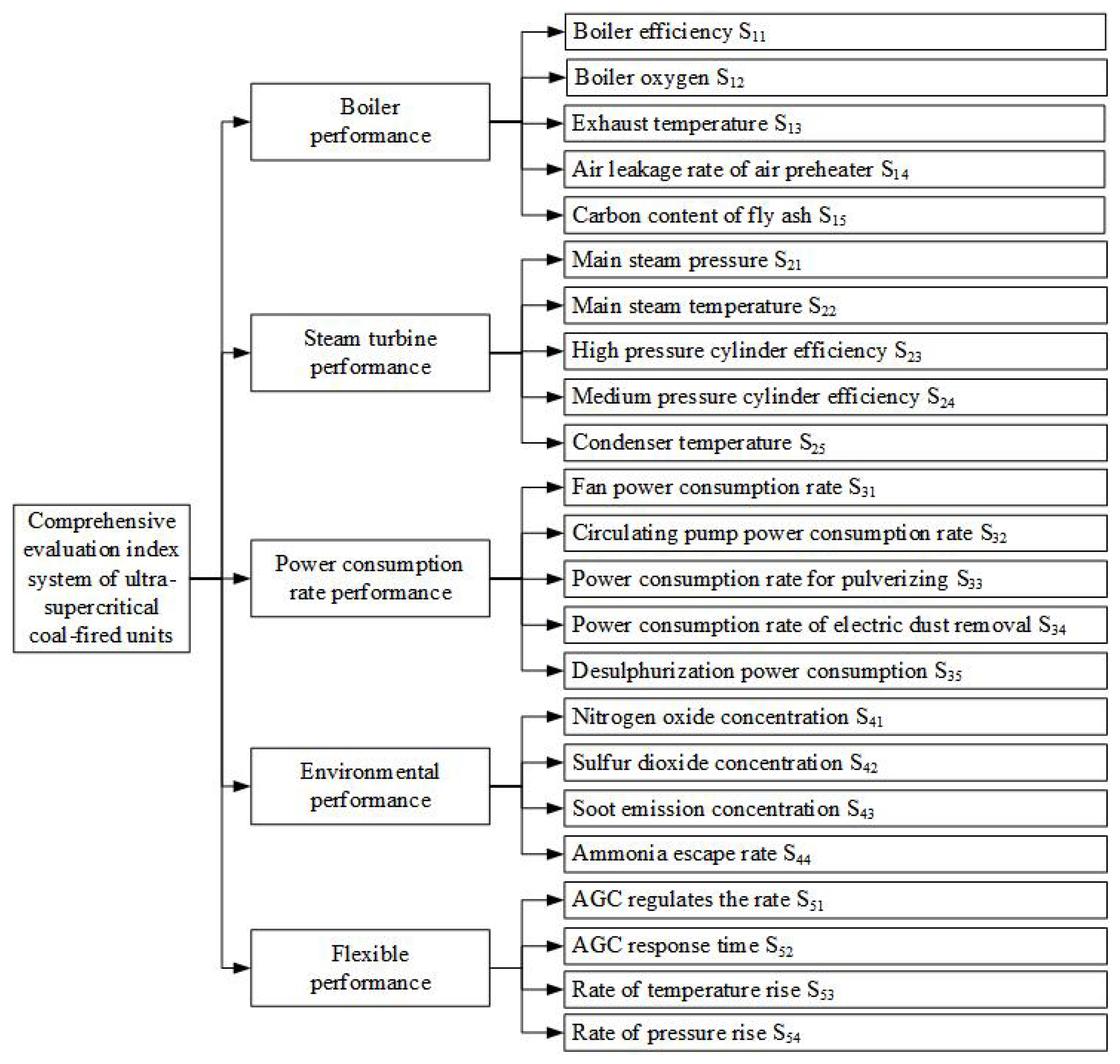
Figure 1. Comprehensive evaluation index system of coal-fired units

Figure 2. The indicators’ combined weights are determined using the CRITIC in various environments.

Figure 3. The indicators’ combined weights are determined using the ICRITIC in various environments.

Figure 4. The indicators’ combined weights are determined using the ICRITIC in various environments.

Table 1. Scale reference table for "time degree".

$θ$	Significance
0.1	Great emphasis on recent data
0.3	Pay more attention to recent data
0.5	Also focus on period data
0.7	Pay more attention to the forward data
0.9	Great emphasis on forward data
0.2, 0.4, 0.6, 0.8	The intermediate case corresponding to the above two adjacent judgments

Table 2. Static evaluation results in winter.

Index	100%THA(±2%)			50%THA(±2%)			Variable load(25%-98%)
Index	$T_{1}$	$T_{2}$	$T_{3}$	$T_{1}$	$T_{2}$	$T_{3}$	$T_{1}$	$T_{2}$	$T_{3}$
$S_{11}$	0.0080	0.0122	0.0111	0.0226	0.0254	0.0161	0.0205	0.0144	0.0099
$S_{12}$	0.6344	0.6577	0.6244	0.6474	0.6134	0.5613	0.7631	0.7522	0.7143
$S_{13}$	0.1462	0.1058	0.1195	0.1131	0.1376	0.1803	0.0908	0.0915	0.0943
$S_{14}$	0.2113	0.2243	0.2449	0.2169	0.2236	0.2423	0.1256	0.1420	0.1816
$S_{15}$	0.0000	0.0000	0.0000	0.0000	0.0000	0.0000	0.0000	0.0000	0.0000
$S_{21}$	0.2178	0.1807	0.0830	0.3461	0.3281	0.2949	0.6262	0.5593	0.6110
$S_{22}$	0.1716	0.1429	0.0471	0.2073	0.1359	0.1073	0.0524	0.0474	0.0302
$S_{23}$	0.1518	0.1213	0.0710	0.1932	0.1636	0.1493	0.0882	0.0859	0.0708
$S_{24}$	0.0350	0.0256	0.0168	0.0417	0.0249	0.0240	0.0781	0.0662	0.0632
$S_{25}$	0.4237	0.5295	0.7821	0.2117	0.3475	0.4244	0.1552	0.2412	0.2248
$S_{31}$	0.0976	0.0713	0.0870	0.0472	0.0231	0.0264	0.1275	0.1198	0.1096
$S_{32}$	0.0292	0.0240	0.2759	0.0282	0.6038	0.5370	0.2553	0.3535	0.4052
$S_{33}$	0.1199	0.0725	0.0982	0.2486	0.0969	0.0953	0.1034	0.0862	0.0782
$S_{34}$	0.2855	0.2772	0.2270	0.3037	0.1224	0.1547	0.2230	0.1937	0.1885
$S_{35}$	0.4677	0.5551	0.3119	0.3723	0.1537	0.1866	0.2908	0.2468	0.2185
$S_{41}$	0.1166	0.1037	0.1366	0.2312	0.1556	0.1950	0.1580	0.1775	0.1903
$S_{42}$	0.4714	0.4768	0.3200	0.2962	0.3261	0.2028	0.4656	0.3767	0.2849
$S_{43}$	0.1274	0.2200	0.2714	0.0740	0.1633	0.1767	0.0983	0.1230	0.1615
$S_{44}$	0.2846	0.1995	0.2720	0.3986	0.3550	0.4255	0.2780	0.3228	0.3634
$S_{51}$	0.0715	0.2632	0.1142	0.2029	0.2231	0.1665	0.1055	0.1226	0.1252
$S_{52}$	0.8677	0.6324	0.7506	0.5780	0.6750	0.6754	0.7611	0.7779	0.7718
$S_{53}$	0.0280	0.0375	0.0718	0.0921	0.0392	0.0613	0.0452	0.0359	0.0384
$S_{54}$	0.0328	0.0669	0.0635	0.1270	0.0628	0.0968	0.0882	0.0635	0.0646

Table 3. Static evaluation results in summer.

Index	90%THA(±2%)			50%THA(±2%)			Variable load(25%-98%)
Index	$T_{4}$	$T_{5}$	$T_{6}$	$T_{4}$	$T_{5}$	$T_{6}$	$T_{4}$	$T_{5}$	$T_{6}$
$S_{11}$	0.0094	0.0063	0.0094	0.0124	0.0130	0.0142	0.0126	0.0071	0.0073
$S_{12}$	0.5838	0.6621	0.5509	0.4771	0.5025	0.5046	0.8002	0.7027	0.6911
$S_{13}$	0.1255	0.1180	0.1371	0.1695	0.1651	0.1645	0.0701	0.0813	0.0848
$S_{14}$	0.2813	0.2135	0.3026	0.3410	0.3194	0.3167	0.1170	0.2089	0.2169
$S_{15}$	0.0000	0.0000	0.0000	0.0000	0.0000	0.0000	0.0000	0.0000	0.0000
$S_{21}$	0.1477	0.1583	0.1712	0.2646	0.1734	0.2239	0.5009	0.4394	0.4787
$S_{22}$	0.0388	0.1104	0.0909	0.0519	0.0640	0.0488	0.0365	0.0485	0.0332
$S_{23}$	0.1113	0.1569	0.1253	0.1448	0.1203	0.1415	0.0920	0.0957	0.0921
$S_{24}$	0.0183	0.0174	0.0229	0.0216	0.0285	0.0276	0.0717	0.0432	0.0495
$S_{25}$	0.6839	0.5571	0.5897	0.5171	0.6138	0.5582	0.2988	0.3732	0.3464
$S_{31}$	0.0920	0.1074	0.0135	0.0501	0.0741	0.0054	0.1269	0.0853	0.0138
$S_{32}$	0.2497	0.1461	0.3647	0.4825	0.2762	0.4340	0.2992	0.3067	0.4155
$S_{33}$	0.1117	0.1728	0.3859	0.1700	0.2238	0.4969	0.0704	0.1087	0.4496
$S_{34}$	0.2487	0.3178	0.1110	0.0833	0.1474	0.0298	0.1841	0.2189	0.0549
$S_{35}$	0.2979	0.2558	0.1249	0.2142	0.2785	0.0340	0.3194	0.2803	0.0662
$S_{41}$	0.1127	0.0819	0.0767	0.1517	0.1315	0.1628	0.1354	0.1211	0.2295
$S_{42}$	0.3424	0.3073	0.3340	0.2378	0.1697	0.2359	0.3122	0.2631	0.2521
$S_{43}$	0.3108	0.4462	0.3592	0.2205	0.3837	0.2845	0.2837	0.3846	0.2985
$S_{44}$	0.2342	0.1647	0.2300	0.3900	0.3151	0.3168	0.2687	0.2312	0.2199
$S_{51}$	0.1622	0.2897	0.1186	0.2748	0.1181	0.0921	0.1380	0.0795	0.0795
$S_{52}$	0.7328	0.5992	0.6849	0.6139	0.7710	0.7752	0.7646	0.7977	0.8362
$S_{53}$	0.0522	0.0420	0.0965	0.0445	0.0331	0.0411	0.0295	0.0294	0.0211
$S_{54}$	0.0528	0.0691	0.1001	0.0669	0.0777	0.0915	0.0680	0.0935	0.0632

Table 4. Results of dynamic comprehensive evaluation.

Index	Winter			Summer
Index	100%THA (±2%)	50%THA (±2%)	Variable load (25%-98%)	90%THA (±2%)	50%THA (±2%)	Variable load (25%-98%)
$S_{11}$	0.0110	0.0198	0.0126	0.0083	0.0136	0.0079
$S_{12}$	0.6367	0.5897	0.7333	0.5913	0.5002	0.7091
$S_{13}$	0.1182	0.1560	0.0929	0.1290	0.1654	0.0816
$S_{14}$	0.2334	0.2326	0.1601	0.2684	0.3208	0.1991
$S_{15}$	0.0000	0.0000	0.0000	0.0000	0.0000	0.0000
$S_{21}$	0.1279	0.3125	0.5955	0.1637	0.2114	0.4683
$S_{22}$	0.0883	0.1285	0.0383	0.0885	0.0541	0.0384
$S_{23}$	0.0962	0.1596	0.0780	0.1335	0.1347	0.0933
$S_{24}$	0.0217	0.0264	0.0661	0.0204	0.0270	0.0500
$S_{25}$	0.6415	0.3661	0.2200	0.5908	0.5708	0.3486
$S_{31}$	0.0829	0.0277	0.1153	0.0450	0.0258	0.0434
$S_{32}$	0.1248	0.4342	0.3660	0.2661	0.3832	0.3616
$S_{33}$	0.0918	0.1126	0.0840	0.2643	0.3462	0.2521
$S_{34}$	0.2508	0.1602	0.1947	0.1869	0.0672	0.1145
$S_{35}$	0.4063	0.1961	0.2370	0.1849	0.1136	0.1517
$S_{41}$	0.1225	0.1859	0.1816	0.0829	0.1505	0.1768
$S_{42}$	0.3887	0.2531	0.3367	0.3261	0.2128	0.2634
$S_{43}$	0.2319	0.1559	0.1391	0.3802	0.3064	0.3239
$S_{44}$	0.2481	0.3978	0.3378	0.2075	0.3256	0.2299
$S_{51}$	0.1499	0.1893	0.1216	0.1740	0.1204	0.0864
$S_{52}$	0.7248	0.6618	0.7724	0.6619	0.7512	0.8136
$S_{53}$	0.0528	0.0569	0.0384	0.0699	0.0388	0.0248
$S_{54}$	0.0599	0.0882	0.0672	0.0823	0.0834	0.0733

Disclaimer/Publisher’s Note: The statements, opinions and data contained in all publications are solely those of the individual author(s) and contributor(s) and not of MDPI and/or the editor(s). MDPI and/or the editor(s) disclaim responsibility for any injury to people or property resulting from any ideas, methods, instructions or products referred to in the content.

© 2024 by the authors. Licensee MDPI, Basel, Switzerland. This article is an open access article distributed under the terms and conditions of the Creative Commons Attribution (CC BY) license (http://creativecommons.org/licenses/by/4.0/).

Copyright: This open access article is published under a Creative Commons CC BY 4.0 license, which permit the free download, distribution, and reuse, provided that the author and preprint are cited in any reuse.

MDPI Initiatives

Important Links

Choose an area of interest and we will send you notifications of new preprints at your preferred frequency.

Disclaimer

Dynamic Comprehensive Evaluation of a 660MW Ultra-Supercritical Coal-Fired Unit Based on Improved Criteria Importance through Inter-criteria Correlation and Entropy Weight Method

Abstract

1. Introduction

2. The Construction of Index System

2.1. Principle of Index System Construction

2.2. Index System of Coal-Fired Units

3. Methods

3.1. Improve CRITIC Method

3.2. Entropy Weight Method

3.3. Combinatorial Weighting

3.4. Aggregation Operator

3.4.1. TOWA Operator

3.4.2. TOWGA Operator

3.4.3. TOWA-TOWGA Hybrid Model

3.5. Determination of Time Weight

4. Results and discussion

4.1. Determination of Combinatorial Weights

4.2. Determination of Combinatorial Weights

5. Conclusions

Author Contributions

Funding

Data Availability Statement

Conflicts of Interest

References

MDPI Initiatives

Important Links

Subscribe