Submitted:
05 February 2024
Posted:
06 February 2024
You are already at the latest version
Abstract
Weak interaction processes continue to be hot topics in fundamental physics research. In this paper, we briefly review some recent advances in the theoretical study of beta and double-beta decays that include both the nuclear and atomic part of these processes. On the nuclear side, we present a statistical approach for the computation of the nuclear matrix elements (NME) for neutrinoless double-beta (0νββ). A range of NME values, the most probable value for NME, and the associated theoretical uncertainty are given. Correlations with other related observables are shown as well. On the atomic side, we first briefly review the methods used to get the electrons’ wave functions. Further, we use them for the computation of some relevant kinematic quantities such as Fermi functions, electron spectra and angular correlation between the emitted electrons. Then, we present applications of these calculations to the experimental data analysis related to the search of the Lorentz invariance violation in two-neutrino double-beta (2νββ) decay and description of the decay rates and decay rate ratios for allowed and unique forbidden electron capture (EC) processes.
Keywords:
beta decay
; double-beta decay
; space phase factors
; nuclear matrix elements
; decay rates
; Lorentz violation
1. Introduction
The study of weak interaction transitions plays an essential role in physics research because they can provide critical information on various hot topics in atomic, nuclear, particle physics, and astrophysics. For example, the study of beta transitions is essential in describing the reactor processes[1], properties of the nuclei far from stability[2], or understanding the evolution of the stars [3,4]. Also, the study of double-beta decay (DBD) offers a broad range of very current topics related to the nuclear structure, validity of some symmetry laws, yet-unknown properties of neutrinos and constraining physics scenarios beyond the Standard Model (SM) [5,6,7,8,9,10].
Beta and double-beta decay rates can be written as a product of an atomic and a nuclear part. The atomic part, namely the phase space factors (PSF), encompasses the perturbation of the movement of the emitted leptons (electrons, protons) due to their interaction with the Coulomb field and electron cloud of the daughter nucleus, while the nuclear part, the nuclear matrix elements (NME) is related to the nuclear structure of the nuclei involved in the decay. For the ) decay channel, a third term appears as follows:
where and are PSF and NME for the and decay modes, is the axial vector coupling constant and is a beyond SM parameter associated with different possible mechanisms that can trigger the decay.
For beta transitions, the probability per unit time that a nucleus with atomic mass A and charge Z decays for a -forbidden -branch is given by [11]:
where g is the weak interaction coupling constant, p is the momentum of -particle, W = is the total energy of -particle and is the maximum -particle energy. = , in decay (Q is the mass difference between initial and final states of neutral atoms). Eq. (2) is written in natural units ( ) so that the unit of momentum is , the unit of energy is , and the unit of time is ℏ /. The shape factors which appear in Eq. (2) are defined as:
where and contains the nuclear matrix elements and , and are bilinear combinations of radial components of the electron wave function.
As seen from the above formulas, in order to reliably predict beta and double-beta decay half-lives, interpret the measured electron spectra, extract information about neutrino properties or constrain different BSM scenarios for decay occurrence, both nuclear and atomic part require accurate computation. The two terms, PSF and NME, are calculated separately with atomic and nuclear methods. NME calculation is a hot topic in the description of the weak interaction processes that lasts for a long time and which is still not satisfactorily solved. For DBD, a second order weak interaction process, this problem is crucial since NME appear in the half-life formulas at a power of two and any uncertainty in the computation is amplified in terms of half-lives prediction. For beta decay the NME calculation is important as well for quantitative predictions of the decay rates and it is not an easy task, since the nuclei undergoing beta transitions belong to different nuclear mass region and have various nuclear structures.
In this paper we give a brief review of some recent advances in the computation of NME for DBD and kinematic quantities such as Fermi functions, electron spectra and angular correlation between electrons relevant for data analyses. In Section 2, we present an analysis and new estimations of the NME for decay. We comment on the present status of the NME computation and briefly present a statistical model aiming to study the stability of NME calculated with interacting Shell model (ISM) method, at small, random variations of some model effective Hamiltonians. Also, we predict a range of the NME values and give the most likely value of it with a predicted theoretical error. In Section 3 we resume different approaches for obtaining the w.f. of the emitted electrons, which are the basic ingredients in the computation of other relevant kinematic quantities for beta and double-beta transitions. In Section 4 we resume the theoretical framework developed for investigating the LIV in decay, while in section 5 we present a study of the electron capture (EC) processes using the Dirac-Hartree-Fock-Slater (DHFS) method. Finally, we end up with conclusions to this review.
2. Nuclear Matrix Elements
The computation of the NME for DBD is a long-standing problem that still needs to be satisfactorily solved. Until recently, their computation was performed with nuclear methods that use phenomenologically effective NN potentials. The most well known are: interaction shell model (ISM) [12,13,14,15,16,17], proton-neutron quasi-random phase approximation (pnQRPA) methods [7,18,19,20,21,22], IBM [23], Energy Density Functional [24], PHFB [25], Coupled-Cluster method (CC) [26], in-medium generator coordinate method (IM-GCM) [27] and valence-space in-medium similarity renormalization group method (VS-IMSRG) [28], were largely discussed over time. The current situation is that there are still significant differences between NME values calculated with different methods [29]). These methods have their strengths or weaknesses, depending on the different approximations on which they are built. These are mainly related to the dimension of the model spaces for the single-particle basis and the number and type of the NN correlations involved in the calculation. For example, pnQRPA, IBM, can use large model spaces for the single-particle states but only a few types of correlations between nucleons, while ISM can use only a restricted model space (only one shell) but includes all types of correlations and preserve the symmetries. As mentioned above, the common feature of these methods is that they all employ phenomenological effective NN potentials in the NME computation. Here, an important aspect is that while pnQRPA derives the NN effective potential from infinite matter using the Brueckner approach and adapts their form by multiplying with specific parameters, ISM uses effective NN potentials built for specific model spaces for different nuclear regions and checks their reliability by comparing the theoretical estimations with the data for other observables in the same nuclear mass region. However, as mentioned above, these methods still give differences between NME values, sometimes calculated with the same method (pnQRPA or ISM), which can amount up to factors of three or more, depending on the specific isotope and values of the input parameters considered in the calculation. Because of these uncertainties, there is a need for more fundamental approaches for the NME computation for DBD. In this regard, there is currently a coherent program for advancing such calculations [30], the main idea being to obtain NME values with minimal dependence on the computational model and provide a quantified theoretical uncertainty. The hope is the progress in developing methods based on particle and nuclear effective field theories (EFT)[31], lattice quantum chromodynamics (QCD) [32], and ab-initio nuclear-many-body techniques [33]. However, the current NME values obtained with these methods are still far from good predictions. Available results are only for NME of [26,34], [35] and [35,36]. In this context, the traditional methods still predict NME values close to the experimental measurements. One missing thing would be finding a reliable range of NME values with a predicted uncertainty to provide experimenters with a better plan to calibrate their set-ups, and interpret the results.
In this context, we propose a statistical analysis of NME and applied it to [37] and Xe [38] isotopes. We only consider the standard light LH neutrino exchange mass mechanism, which is most likely to contribute to the decay process. Details of these models can be found in the cited references and we give here only the relevant ingredients. We employed three independent effective Hamiltonians for each isotope, suitable for each nuclear mass region, namely FPD6, GXPF1A, KB3G for and SVD, GCN5082, jj55t for and investigated the effect of small, random variations of the shell model effective Hamiltonians on NME. These effective Hamiltonians are described by a small number of single-particle energies and a finite number of two-body matrix elements. The wave functions produced by these Hamiltonian can also be used to describe and predict other observables, such as the electromagnetic and Gamow-Teller (GT) transition probabilities, nucleon occupation probabilities, spectroscopic factors, etc, using relative simple changes of the transition operators in terms of effective charges and quenching factors. These effective charges and quenching factors are calibrated to the existing data. For NME, such calibrations are not yet possible due to the lack of data. However, different existing effective Hamiltonians for nuclei involved in a given decay produce smaller ranges of the NME values.
The main goals of our study were: (a) for each starting effective Hamiltonian find correlations between NME and the other observables that are accessible experimentally; (b) find theoretical ranges for each observable; (c) establish the shape of different distributions for each observable and starting Hamiltonians; (d) use this information to find weights of contributions from different starting Hamiltonians to the "optimal" distribution of the NME; (e) find an "optimal" value of the NME and its predicted probable range (theoretical error). We refer further to the relevant results obtained for , which is one of the most experimentally studied isotope.
For example, in Table 1, we present the correlations that we found between several relevant observables. The notations are obvious and the letters "P" and "D" added to the name of the observables denote "parent" and "daughter" nuclei. The calculations were done with the ISM in the jj55 model space consisting of the 0g7/2, 1d5/2, 1d3/2, 2s1/2 and 0h11/2 orbitals that assume as a core, covering the sector of the nuclear chart between (N, Z) = 50-82. We generated 1000 effective Hamiltonians from each starting Hamiltonian via random perturbations within the range of to their two-body matrix elements (TBME). The methodology of calculating the NME () within ISM was extensively described elsewhere [13], and we do not repeat here the details of the calculation. First of all, as expected, and are strongly correlated, so an accurate computation of may help in the computation of . Overall, from Table 1, one can see that the SVD starting Hamiltonian produces NMEs that are closest to the experimental value, thus needing the least amount of quenching when compared to those of GCN5082 or jj55t. For the PGT and DGT, one observes that the SVD results are closest to the experimental data for the parent nucleus, overestimating the result by much less than GCN5082 and jj55t. However, for the daughter’s GT, GCN5082 was best, with SVD underestimating the result the most. For PB(E2)↑ and DB(E2)↑, SVD shows values closest to the experiment. The excitation energies are better described by GCN5082, in large part because the GCN5082 starting Hamiltonian was fine-tuned with data for more nuclei and energy levels than SVD and jj55t. Interestingly, the correlations between the NME and the strengths of the parent and daughter GT transitions to the first state in are significantly reduced, while the correlation with the NME is very strong. One explanation for this phenomenon could be related to the fact that the product of the GT matrix elements describing transitions to the first state in does not significantly contribute to the total sum of all excited states in the intermediate nucleus.
Figure 1 (taken from [38]) shows the probability distribution functions (PDF) for the three starting effective Hamiltonians and their weighted sum. To calculate each PDF, we use the Bayesian approach, described in detail in [38]. Based on our statistical analysis summarized in this Figure, one can infer that with 90 % confidence, the NME lies between 1.55 and 2.65, with a mean value of about 1.99 and a standard deviation of 0.37.
3. Electron Wave Functions
To calculate the kinematic part of the beta and double-beta transitions, one needs to get reliable wave functions (w.f.) for the emitted electrons, which includes their interaction with the Coulomb-type field given by the protons and electronic cloud of the daughter nucleus. They are the essential ingredients to compute Fermi functions, PSF, electron spectra, decay rates and all other needed kinematic quantities (experimentally measurable). Until now, several methods were used to calculate the electron w.f. for continuous and bound states to describe the beta and double-beta transitions. We resume here some of them.
Approach A. In a non-relativistic treatment used in early calculations of the DBD decay rate [39,40], the electron w.f were taken as solutions of the Schrödinger equation in a Coulomb potential given by a point-like nucleus, and the Fermi function was built as a scattering solution for a point charge to a plane wave, evaluated at the origin:
where , "+" ("-") are for electrons (positrons), is the fine structure constant, is the energy of the outgoing lepton and is its momentum.
This approximation fails badly for heavy nuclei, but it has the advantage that the DBD rate can be integrated analytically, resulting in a polynomial in powers of Q-value.
Approach B. In a relativistic treatment, the electron w.f. were obtained as solutions of the Dirac equation with a Coulomb potential given by a point charge, and the Fermi function can be written as: [7]
with
with the same sign convention as above. R is the cut-off radius in the evaluation of the Dirac equation, which is taken to match the radius of the daughter nucleus (i.e., fm). In another version of this relativistic treatment, the electron w.f. and Fermi functions were obtained by solving a Dirac equation with Coulomb potential given by a spherical finite-size charge (nucleus). The Fermi function can be also obtained in an analytical form by retaining the first term in a series expansion of the electron w.f. in spherical functions [5].
These analytical forms of the Fermi functions were extensively used for computing DBD half-lives in many works [5,7]. We also note that the screening effect, which proved to be important, was not included in both of these methods.
Approach C
The Fermi functions are built from the exact electron w.f. [41], which are obtained by solving numerically the Dirac equation in a spherical Coulomb potential given by a finite-size charged nucleus, and including the electron screening effect. The details of the calculations can be found in refs. [41,42,43].
where fm is the nuclear radius. To compute the Fermi function and PSF, we have to obtain the electron factors [6]:
with
which are related to the electron radial w.f., f and g:
which g and f are the radial solutions of the above Dirac equation.
We note that in ref. [41] the Coulomb potential () from the Dirac equation has the form given by a finite size charged nucleus while in refs. [42,43] the Coulomb potential was built from a realistic distribution of the protons in the daughter nucleus. The difference between the Coulomb-type potentials can be seen in Figure 2 from [42]. Notably, the differences in the PSF values for DBD with double-electron emission, computed with the two types of Coulomb potentials, amount at most to a few percent, while for other decay channels the differences may be relevant. We mention that in both of these methods, the screening effect was introduced as a renormalization of the Coulomb potential with a Thomas Fermi function [41,42,43]. To obtain the radial electron/positron w.f. the Dirac equation was solved using the subroutines package RADIAL [44].
There are differences when applying the approaches (A-C) to calculating the electron spectra. For example, in Figure 2 is presented the summed energy electron spectra for the decay of and its deviation due to LIV effects, with methods A, B and C as is specified in the caption. One can see a large difference between the non-relativistic and relativistic treatments and between the B and C approaches.
Approach D In this approach, the electron w.f. are obtained with the DHFS method using a Coulomb potential given by a nucleus with a diffuse surface. More details can be found in [46]. This method also gives accurate calculations of the kinematic quantities that appear in the beta and double-beta decay studies and better applies to EC processes, as we will se in section 5. The Dirac equation is solved iteratively: one starts with predefined w.f. and computes the potential, then the equation is solved to obtain the new w. f., and the potential is recalculated until a convergence criterion is reached. The DHFS method constructs the potential as a sum of three components: the nuclear potential generated by a nucleus with a realistic Fermi proton charge distribution, the electronic potential as a mean field generated by the charge distribution of the electronic cloud and the exchange potential assuring the asymptotic condition at as [44]:
In this approach, the screening effect is considered by including the mean-field treatment of the electronic potential component, .
4. Lorentz Violation in the Neutrino Sector
Lorentz invariance violation (LIV) is a current topic that joins the increasing effort to test the SM limits. The theoretical framework which introduces LIV contributions is the SM extension (SME) theory [47], including operators that break Lorentz invariance for all the particles in the SM. In particular, the neutrino sector of SME provides the theoretical framework for a rich phenomenology for searching evidence of LIV [48]. The first experimental searches were done in the neutrino oscillations experiments [49–51]. Another LIV signature in the neutrino sector can appear due to the so-called counter-shaded effects associated with the oscillation-free operators of mass dimension three, which cannot be investigated in these experiments. Beta and double-beta decays offers the possibility to investigate the LIV effects related to the time-like (isotropic) component of this oscillation-free operator whose size is controlled by the coefficient . In refs. [52] the LIV effects in decay were calculated for the summed energy spectra of electrons employing a non-relativistic approximation for the electron radial w.f. Currently, the accuracy required in the DBD experiments far exceeds this approximation. Therefore, precise computation of the electron spectra is needed. Recently, experiments like EXO-200 [53], CUPID-0 [54], NEMO-3 [55], CUORE [56], GERDA[57] have provided limits for the parameter from the analysis of the summed energy spectra of electrons in decays, using theoretical predictions of these spectra performed with approximate methods of calculation. In [45], we examined the effects of LIV on summed energy spectra of electrons and quantities related to them using Fermi functions built with exact electron w.f. (Approach C is described in section 3). First, we derived the complete formalism for LIV analyses in decay. For the sake of consistency, we give here the final formulas, while the detailed derivation of them can be found in refs.[45,58,59].
The DBD decay rate can be written as a sum of the SM decay rate and its deviation due to LIV [52]:
As it was already mentioned earlier, the decay rate can be written as a product of NME and PSF.
Since the nuclear part does not contain neutrinos, and the LIV effects appear through the change of the neutrino momentum, only affected are the phase space factors , where the neutrino energy and momentum appear explicitly. The angular differential DBD rate within the SM can be expressed as [5,58]:
A similar formula can be written within SME [58]:
The spectrum part ( ) and the angular correlation part () of the decay rate can be obtained by integrating Eqs. (17)-(18) over the lepton energies. C is a constant, G and H are the PSF associated with the two decay rate parts, is the angle between the two emitted electrons, is the angular correlation coefficient defined as the ratio of and decay rates, and is the coefficient that governs the size of the LIV effects. Besides the summed energy electron spectra, one can also define another quantity related to the summed energy electron spectra that can be compared with experimental measurements, :
The PSF expressions and their deviations due to LIV can be gathered as follows [58]:
Until now, the LIV investigations have been done in several DBD experiments and are limited to extracting the LIV coefficient from the analysis of the summed electron spectra. The deviation of the summed energy electron spectrum due to LIV effects was presented in section 3, Figure 3 (taken from [45]), and it is displayed as a shift of the maximum of the spectrum to higher energy. This deviation was computed using improved electron w.f. (Method C) and up-dated Q-values [45]). In our next works [58,59], we computed the LIV deviations of the summed energy electron spectra for all DBD isotopes of experimental interest. Then, we also extended our study to the single electron spectra (Figure 4) and electron angular correlation (Figure 5b), providing thus additional possible LIV investigations by analyzing these spectra as well.
Single electron spectra can also undergo LIV deviations, but they can only be investigated in experiments using detectors with tracking systems of individual electrons. Also, we suggested the analysis of the quantities (Eq. 20) in the vicinity of the Q-values, where larger LIV deviations of the SM spectra would be expected, as seen in Figure 5. By comparing the electron and angular correlation spectra computed with and without LIV contributions, one can get information about the observability of the LIV effects with the current experimental statistics. Further, we proposed a new, alternative method to constrain the LIV parameter. This consists in comparing the measured value of the angular correlation coefficient k, which can be determined in the DBD experiments with electron tracking systems [60] by using the forward-backwards asymmetry, with its theoretical value. Eq. 22 shows how the coefficient can be determined by measuring the balance between the number of electrons emitted forward and backward.
Finally, we mention that the search for LIV effects will has a greater chance of success in the future DBD experiments as the statistics for the DBD events, especially in the vicinity of the Q-values, will improve. Also, there are more chances to be observed in DBD experiments with tracking detectors for individual electrons. We hope our works have strenghtened the theoretical support necessary for further research into LIV effects in DBD.
5. Decay rates for EC processes
Electron capture processes manifest across a broad spectrum of isotopes [61] and play a crucial role in practical applications such as radionuclide metrology [62] and nuclear medicine [63]. In these applications, the relevance is that most Auger electrons emitted during EC processes possess kinetic energies in the range of a few keV, enabling precise deposition within a confined area, thus allowing targeted irradiation of tumour sites. EC processes also play a determinant role in fundamental physics research like nuclear astrophysics [64] and Dark Matter and DBD experiments for accurate background characterization [65]. Notably, in the precise measurement of the in , a critical background contribution emerges from EC, as its decay peak closely aligns with that of the peak [66]. That is why there is a great interest in understanding these processes better, and in this regard, theoretical support is crucial.
In this context, we develop a program to calculate EC processes for a wide nuclear region, A=7-204 [68]. We give here only the main ingredients of our work, highlighting the improvements and the obtained results. The decay rate () for allowed and unique-forbidden transition is defined as [67]:
where is the Coulomb amplitude, represents the energy of the emitted neutrino, denote the overlap and exchange corrections and is the shake-up and shake-off correction. The angular momentum of the electron capture transition is represented as L, and contains the nuclear matrix element. The total energy of the captured electron is given by , with the binding energy and the electron rest-mass energy. The momentum of the bound electron is obtained as , and the momentum of the emitted neutrino is denoted . The relative occupation number is obtained as .
The decay energy Q is calculated as the atomic mass different between the initial and final atom:
where and are the and X-ray radiation energies released by the final nucleus/ atom. The total binding energy of the electronic cloud is represented as .
More details can be found in [68]. The most important elements of the calculation are the electron w.f., the single-electron binding energies and the total electron binding energies. We utilize the DHFS self-consistent framework for their computation. The framework is validated by comparing the single-electron energies and the total binding energies we obtained with the experimental ones, thus observing a good agreement. By comparison, other models artificially induce the convergence of energies to specific values for each atomic number. A mention-worthy approach is the BETASHAPE (BS) program [69]. One significant improvement of our work is a refined energy balance in Eq. 24. We consider the whole system (the initial and final atom), not only the nuclei and the captured electron. The binding energies of electrons that do not participate directly in the decay (spectator electrons) change between the initial and final state. This has an important effect on the energy balance, affecting the neutrino energy, which enters directly in the decay rate Eq. 23. This approach yielded improved agreement with experimental values for EC fractions, particularly in low-energy transitions.
For our calculations, we computed the w. f. of all electrons in the initial atom in the ground state configuration and in the final atom, considering all possible configurations after an electron is captured. Then, we computed the shake-up and shake-off correction and the exchange and overlap correction using the w.f.s of the electrons.
In Table 2 (taken from [68]), we present a comparison of the decay constant ratios for multiple shells. We employ the use of ratios in order to reduce the NME, thus obtaining measurable quantities independent of the nuclear model. We outline a few important cases compared to other experimental (RD) [71] and theoretic results. The experimental values marked with are taken from [70]. We also compare our results with other results from [70] computed using a self-interaction-corrected model, the Krieger-Li-Iafrate (KLI) [72]. In Table 2 we present five allowed transitions Be, Mn, Fe, Cd, I, a first unique forbidden transition Ca and a second unique transition La.
We noted deviations from experimental values below 2% for the ratios across all models, increasing to 12% for captures from higher shells. The BS model and our model consistently provided the most accurate values. Additionally, our model’s validity was tested by comparing theoretical predictions to experimental values across a wide range of atomic numbers and transition energies, revealing excellent agreement (below two standard deviations) in most cases.
Lastly, we emphasize that refined energetics contribute to improved agreement between experimental and theoretical EC ratios, particularly in low-energy transitions. This characteristic holds potential implications for determining the neutrino mass scale from electron capture processes. Our findings have significant implications for future studies in the EC field and related nuclear physics and astrophysics applications.
6. Conclusions
We briefly reviewed some recent advances in the theoretical study of beta and double-beta decays. A statistical approach for determining the NME for is presented on the nuclear side. We studied the stability of the NME values against small, random variations of some effective Hamiltonians used in the computation and their correlation with other observables that are accessible experimentally. From this statistical study, we predicted a theoretical range of the NME values and determined an optimal NME value together with a predictable error. On the atomic side, we briefly reviewed the methods for getting the electron w.f. . Then, we use them to compute relevant, measurable quantities for the data analysis in beta and double-beta decay experiments. First, we deduced the theoretical formulas for electron spectra deviations and angular correlation deviations in decay due to LIV. We proposed the search of possible LIV effects in the summed electron energy and single electron spectra and angular correlation, as well as a new, alternative method to constrain the coefficient that governs the size of the LIV effects. Then, we presented a formalism based on the DHFS approach to compute decay rates and decay ratios from atomic multi-shells, for allowed and unique forbidden EC processes. Our calculations display a good agreement with experimental data. We hope, the results reviewed in this paper represent relevant advances that can improve data analyses in beta and double-beta decay experiments.
Author Contributions
“Conceptualization, S.S.; methodology, S.S., V.S.; software, V.S.; validation, S.S.; preparation S.S and V.S.; draft preparation V.S.; visualization, V.S.; review and editing, S.S.; project administration, S.S.; All authors have read and agreed to the published version of the manuscript.”
Funding
This work was supported by the Romanian Ministry of Research, Innovation and Digitization, project PNRR-I8/C9-CF264, Contract No. 760.100
Institutional Review Board Statement
“Not applicable”
Informed Consent Statement
“Not applicable”
Data Availability Statement
No new data were created or analyzed in this study. Data sharing is not applicable to this article
Conflicts of Interest
“The authors declare no conflicts of interest.” “The funders had no role in the design of the study; in the collection, analyses, or interpretation of data; in the writing of the manuscript; or in the decision to publish the results”.
References
- A. Algora et al. Beta-decay studies for applied and basic nuclear physics. Eur. Phys. J. A 2021, 57, 83. [CrossRef]
- A. C. Mueller, and B. M. Sherrill. Nuclei at the Limits of Particle Stability. Annual Review of Nuclear and Particle Science 1993, 43, 529–583. [CrossRef]
- K. Langanke, and M.Wiescher. Nuclear reactions and stellar processes. Rep. Prog. Phys. 2001, 64, 1657. [CrossRef]
- F.-K. Thielemann et al. The r-, p-, and νp-Process. J. Phys.: Conf. Ser. 2010, 202, 012006. [CrossRef]
- M. Doi, T. Kotani, E. Takasugi. Double-beta decay and Majorana neutrino. Prog. Theor. Phys. Suppl. 1985, 83, 1. [CrossRef]
- T. Tomoda. Double beta decay. Rep. Prog. Phys. 1991, 54, 53. [CrossRef]
- J. Suhonen, O. Civitarese. Weak-interaction and nuclear-structure aspects of nuclear double beta decay. Physics Reports 1998, 300, 123–214. [CrossRef]
- J. D. Vergados, H. Ejiri, F. Simkovic. Theory of neutrinoless double-beta decay. Rep. Prog. Phys. 2012, 75, 106301. [CrossRef] [PubMed]
- M. J. Dolinski, A.W. P. Poon, andW. Rodejohann. Neutrinoless Double-Beta Decay: Status and Prospects. Annu. Rev. Nucl. Part. Sci. 2019, 69, 219–251. [CrossRef]
- A. Barabash. Double Beta Decay Experiments: Recent Achievements and Future Prospects. Universe 2023, 9(6), 290. [CrossRef]
- N. B. Gove and M. J. Martin. LOG-f TABLES FOR BETA DECAY. NUCLEAR DATA TABLES 1971, 10, 205. [CrossRef]
- E. Caurier, G. Martínez-Pinedo, F. Nowacki, A. Poves, and A. P. Zuker. The shell model as a unified view of nuclear structure. Rev. Mod. Phys. 2005, 77, 427. [CrossRef]
- M. Horoi, S. Stoica. Shell model analysis of the neutrinoless double-β decay of 48Ca. Phys. Rev. C 2010, 81, 024321. [CrossRef]
- M. Horoi, and B. A. Brown. Shell-Model Analysis of the 136Xe Double Beta Decay Nuclear Matrix Elements. Phys. Rev. Lett. 2013, 110, 222502. [CrossRef] [PubMed]
- M. Horoi, and A. Neacsu. Shell model predictions for 124Sn double-β decay. Phys. Rev. C 2016, 93, 024308. [CrossRef]
- A. Neacsu, and M. Horoi. Shell model studies of the 130Te neutrinoless double-β decay. Phys. Rev. C 2015, 91, 024309. [CrossRef]
- R. A. Sen’kov and M. Horoi. Accurate shell-model nuclear matrix elements for neutrinoless double-β decay. Phys. Rev. C 2014, 90, 051301(R). [CrossRef]
- D.-L. Fang, A. Faessler, V. Rodin, and F. Šimkovic. Neutrinoless double-β decay of deformed nuclei within quasiparticle random-phase approximation with a realistic interaction. Phys. Rev. C 2011, 83, 034320. [CrossRef]
- M. Kortelainen and J. Suhonen. Improved short-range correlations and 0νββ nuclear matrix elements of 76Ge and 82Se. Phys. Rev. C 2007, 75, 051303(R). [CrossRef]
- V. Rodin, A. Faessler, F. Simkovic, and P. Vogel. Assessment of uncertainties in QRPA 0νββ-decay nuclear matrix elements. Nucl. Phys. A 2006, 766, 107. [CrossRef]
- F. Šimkovic, G. Pantis, J. D. Vergados, and A. Faessler. Additional nucleon current contributions to neutrinoless double β decay. Phys. Rev. C 1999, 60, 055502. [CrossRef]
- S. Stoica and H. Klapdor-Kleingrothaus. Critical view on double-beta decay matrix elements within Quasi Random Phase Approximation-based methods. Nucl. Phys. A 2001, 694, 269. [CrossRef]
- J. Barea, and F. Iachello. Neutrinoless double-β decay in the microscopic interacting boson model. Phys. Rev. C 2009, 79, 044301. [CrossRef]
- T. R. Rodriguez and G. Martinez-Pinedo. Energy Density Functional Study of Nuclear Matrix Elements for Neutrinoless ββ Decay. Phys. Rev. Lett. 2010, 105, 252503. [CrossRef] [PubMed]
- P. K. Rath et al. Neutrinoless ββ decay transition matrix elements within mechanisms involving light Majorana neutrinos, classical Majorons, and sterile neutrinos. Phys. Rev. C 2013, 88, 064322. [CrossRef]
- S. Novario et al. Coupled-Cluster Calculations of Neutrinoless Double-β Decay in 48Ca. Phys. Rev. Lett. 2021, 126, 182502. [CrossRef]
- J. J. Griffin, and J. A. Wheeler. Collective Motions in Nuclei by the Method of Generator Coordinates. Phys. Rev. 1957, 108, 311. [CrossRef]
- S. R. Stroberg, H. Hergert, S. K. Bogner, and J. D. Holt. Nonempirical Interactions for the Nuclear Shell Model: An Update. Annual Review of Nuclear and Particle Science 2019, 69, 307–362. [CrossRef]
- J. Engel, J. Menéndez. Status and future of nuclear matrix elements for neutrinoless double-beta decay: A review. Rep. Prog. Phys. 2017, 80, 046301. [CrossRef]
- V. Cirigliano et al. Towards precise and accurate calculations of neutrinoless double-beta decay. J. Phys. G 2022, 49, 120502. [CrossRef]
- V. Cirigliano et al. New Leading Contribution to Neutrinoless Double-β Decay. Phys. Rev. Lett. 2018, 120, 202001. [CrossRef]
- X. Feng, L.-C. Jin, Z.-Y. Wang, and Z. Zhang. Finite-volume formalism in the 2HI+HI→2 transition: An application to the lattice QCD calculation of double beta decays. Phys. Rev. D 2021, 103, 034508. [CrossRef]
- Z. Davoudi, and S. V. Kadam. Path from Lattice QCD to the Short-Distance Contribution to 0νββ Decay with a Light Majorana Neutrino. Phys. Rev. Lett. 2021, 126, 152003. [CrossRef]
- J. M. Yao et al. Ab Initio Treatment of Collective Correlations and the Neutrinoless Double Beta Decay of 48Ca. Phys. Rev. Lett. 2020, 124, 232501. [CrossRef] [PubMed]
- A. Belley et al. Ab Initio Neutrinoless Double-Beta Decay Matrix Elements for 48Ca, 76Ge, and 82Se. Phys. Rev. Lett. 2021, 126, 042502. [CrossRef] [PubMed]
- D. Patel, P. C. Srivastava, V. K. B. Kota, and R. Sahu. Large-scale shell-model study of two-neutrino double beta decay of 82Se, 94Zr, 108Cd, 124Sn, 128Te, 130Te, 136Xe, and 150Nd. Nucl. Phys. A 2024, 1042, 122808. [CrossRef]
- M. Horoi, A. Neacsu, S. Stoica. Statistical analysis for the neutrinoless double-β-decay matrix element of 48Ca. Phys. Rev. C 2022, 106, 054302. [CrossRef]
- M. Horoi, A. Neacsu, S. Stoica. Predicting the neutrinoless double-β-decay matrix element of 136Xe using a statistical approach. Phys. Rev. C 2023, 107, 045501. [CrossRef]
- E. J. Konopinski. The theory of beta radio activity; Clarendon P.: Oxford, United Kingdom, 1996.
- H. Primakoff and S. P. Rosen. Double beta decay. Rep. Prog. Phys. 1959, 22, 121. [CrossRef]
- J. Kotila, F. Iachello. Phase-space factors for double-β decay. Phys. Rev. C 2012, 85, 034316. [CrossRef]
- M. Mirea, T. Pahomi, and S. Stoica. Values of the Phase Space Factors Involved in Double Beta Decay. Romanian Reports in Physics 2015, 67, 872. [CrossRef]
- S. Stoica and M. Mirea. New calculations for phase space factors involved in double-β decay. Phys. Rev. C 2013, 88, 037303. [CrossRef]
- F. Salvat and J. M. Fernández-Varea. radial: A Fortran subroutine package for the solution of the radial Schrödinger and Dirac wave equations. Comput. Phys. Commun. 2019, 240, 165. [CrossRef]
- O. Niţescu, S. Ghinescu, and S. Stoica. Lorentz violation effects in 2νββ decay. J. Phys. G 2020, 47, 055112. [CrossRef]
- O. Niţescu, R. Dvornický, and F. Šimkovic. Exchange correction for allowed β decay. Phys. Rev. C 2023, 107, 025501. [CrossRef]
- D. Colladay, and V. A. Kostelecký. Lorentz-violating extension of the standard model. Phys. Rev. D 1998, 58, 116002. [CrossRef]
- V. A. Kostelecký and M. Mewes. Lorentz and CPT violation in the neutrino sector. Phys. Rev. D 2004, 70, 031902(R). [CrossRef]
- A. A. Aguilar-Arevalo et al. (MiniBooNE Collaboration). Test of Lorentz and CPT violation with short baseline neutrino oscillation excesses. Phys. Lett. B 2013, 718, 1303–1308. [CrossRef]
- K. Abe et al. (Super-Kamiokande Collaboration). Test of Lorentz invariance with atmospheric neutrinos. Phys. Rev. D 2015, 91, 052003. [CrossRef]
- P. Adamson et al. (The MINOS Collaboration). Search for Lorentz invariance and CPT violation with muon antineutrinos in the MINOS Near Detector. Phys. Rev. D 2012, 85, 031101. [CrossRef]
- J. S. Díaz. Limits on Lorentz and CPT violation from double beta decay. Phys. Rev. D 2014, 89, 036002. [CrossRef]
- J. B. Albert et al. (EXO-200 Collaboration). First search for Lorentz and CPT violation in double beta decay with EXO-200. Phys. Rev. D 2016, 93, 072001. [CrossRef]
- O. Azzolini et al. First search for Lorentz violation in double beta decay with scintillating calorimeters. Phys. Rev. D 2019, 100, 092002. [CrossRef]
- R. Arnold et al. Detailed studies of 100Mo two-neutrino double beta decay in NEMO-3. Eur. Phys. J. C 2019, 40, 440. [CrossRef]
- C. Brofferio, O. Cremonesi, and S. Dell’Oro. Neutrinoless Double Beta Decay Experiments With TeO2 Low-Temperature Detectors. Front. Phys. 2019, 7, 86. [CrossRef]
- L. Pertoldi. earch for Lorentz and CPT symmetries violation in double-beta decay using data from the GERDA experiment. Ph. D. thesis, Universita degli Studi di Padova, 2017.
- S. Ghinescu, O. Niţescu, and S. Stoica. Probing Lorentz violation in 2νββ using single electron spectra and angular correlations. Phys. Rev. D 2022, 105, 055032. [CrossRef]
- O. Niţescu, S. Ghinescu, M. Mirea, and S. Stoica. Probing Lorentz violation in 2νββ using single electron spectra and angular correlations. Phys. Rev. D 2021, 103, L031701. [CrossRef]
- R. Arnold et al. Probing new physics models of neutrinoless double beta decay with SuperNEMO. Eur. Phys. J. C 2010, 70, 927. [CrossRef]
- J. M. Gates et al. Synthesis of rutherfordium isotopes in the 238U(26Mg, xn)264-xRf reaction and study of their decay properties. Phys. Rev. C 2008, 77, 034603. [CrossRef]
- R. Broda, P. Cassette, and K. Kossert. Radionuclide metrology using liquid scintillation counting. Metrologia 2007, 44, S36. [CrossRef]
- E. Bezak, B. Q. Lee, T. Kibédi, A. E. Stuchbery, and K. A. Robertson. Auger radiation targeted into DNA: A therapy perspective. Eur. J. Nucl. Med. Mol. Imaging 2006, 33, 1352. [CrossRef] [PubMed]
- K. Langanke, G. Martínez-Pinedo, and R. G. T. Zegers. Electron capture in stars. Rep. Prog. Phys. 2021, 84, 066301. [CrossRef]
- M. Faverzani et al. The HOLMES Experiment. J. Low Temp. Phys. 2016, 184, 922. [CrossRef]
- E. Aprile et al. (XENON Collaboration). Double-weak decays of 124Xe and 136Xe in the XENON1T and XENONnT experiments. Phys. Rev. C 2022, 106, 024328. [CrossRef]
- W. Bambynek et al. Orbital electron capture by the nucleus. Rev. Mod. Phys 1977, 49, 77. [CrossRef]
- V. A. Sevestrean, O. Niţescu, S. Ghinescu, and S. Stoica. Self-consistent calculations for atomic electron capture. Phys. Rev. A 2023, 108, 012810. [CrossRef]
- X. Mougeot. BetaShape: A new code for improved analytical calculations of beta spectra. EPJ Web of Conferences 2017, 146, 12015. [CrossRef]
- X. Mougeot et al. Influence of the atomic modeling on the electron capture process. arXiv:2111.15321.
- Atomic and Nuclear data - LABORATOIRE NATIONAL HENRI BECQUEREL. Available online: Http://www.lnhb.fr/home/nuclear-data/nuclear-data-table/.
- J. B. Krieger, Yan Li, and G. J. Iafrate. Systematic approximations to the optimized effective potential: Application to orbital-density-functional theory. Phys. Rev. A 1992, 46, 5453. [CrossRef]
Figure 1.
PDFs of neutrinoless NME distribution for the gen5082, jj55t, and SVG Hamiltonians, and their weighted sum [38].
Figure 1.
PDFs of neutrinoless NME distribution for the gen5082, jj55t, and SVG Hamiltonians, and their weighted sum [38].
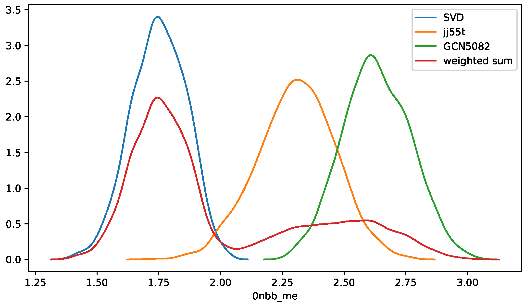
Figure 2.
Realistic proton density for Sm [42]
Figure 2.
Realistic proton density for Sm [42]
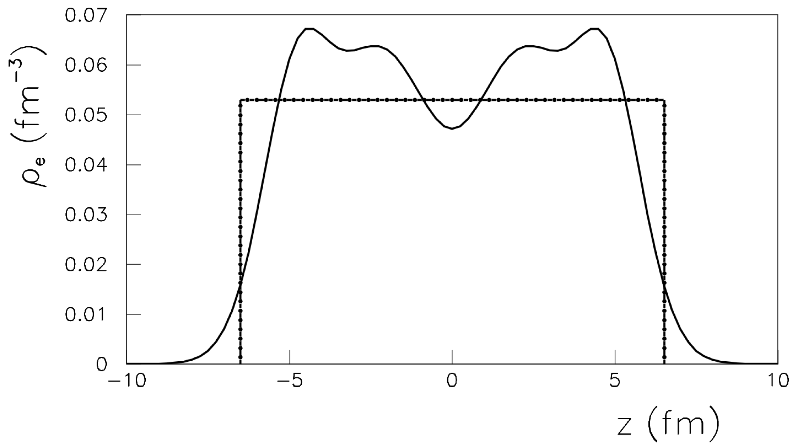
Figure 3.
Summed energy spectra of electrons in decay (a) and deviations due to LIV (b) for Xe [45].
Figure 3.
Summed energy spectra of electrons in decay (a) and deviations due to LIV (b) for Xe [45].
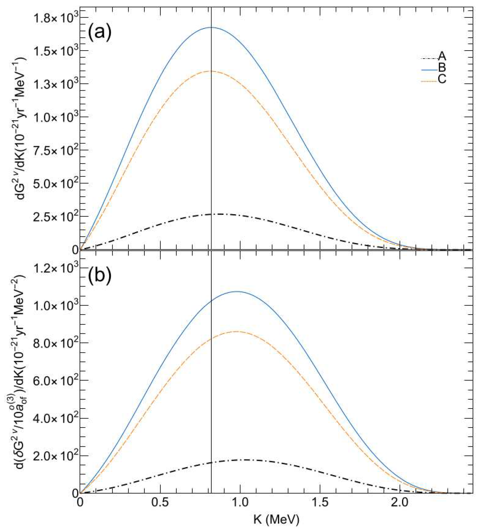
Figure 4.
Normalized single electron spectra for Xe ; SM with solid line and the LIV first-order corrected with dashed line [58].
Figure 4.
Normalized single electron spectra for Xe ; SM with solid line and the LIV first-order corrected with dashed line [58].
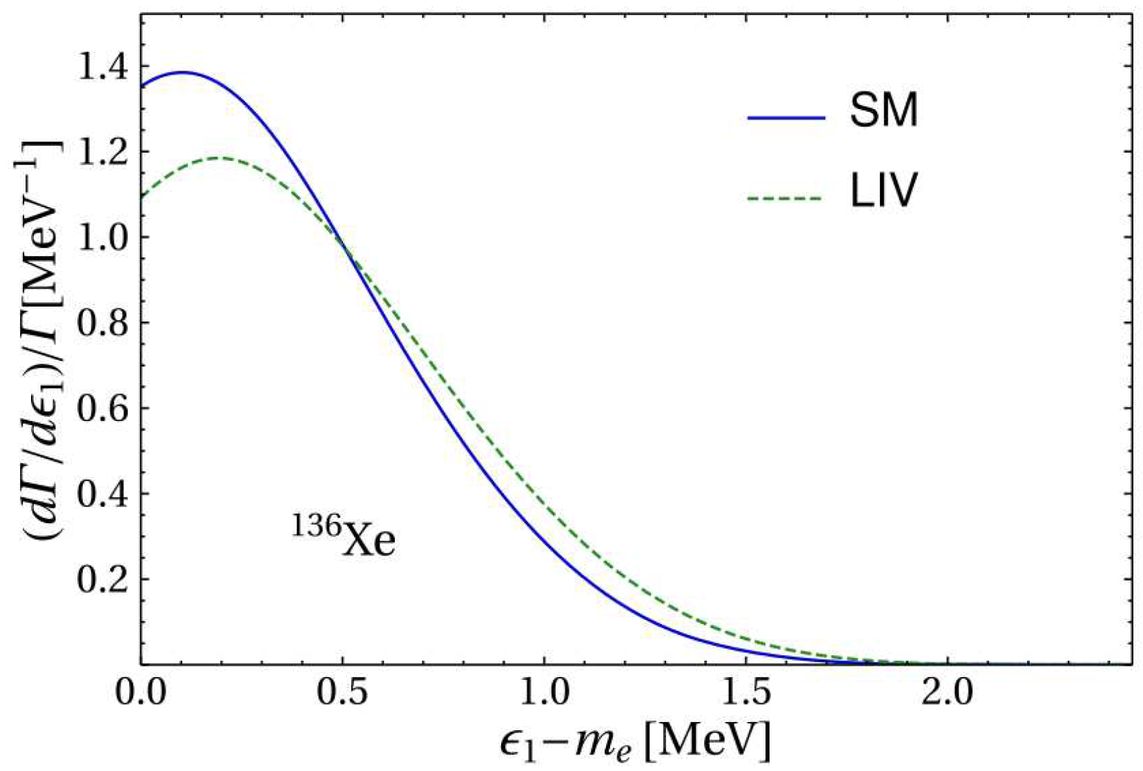
Figure 5.
Both figure are form ref. [59] (dashed for upper limit and dot-dashed for lower limit)
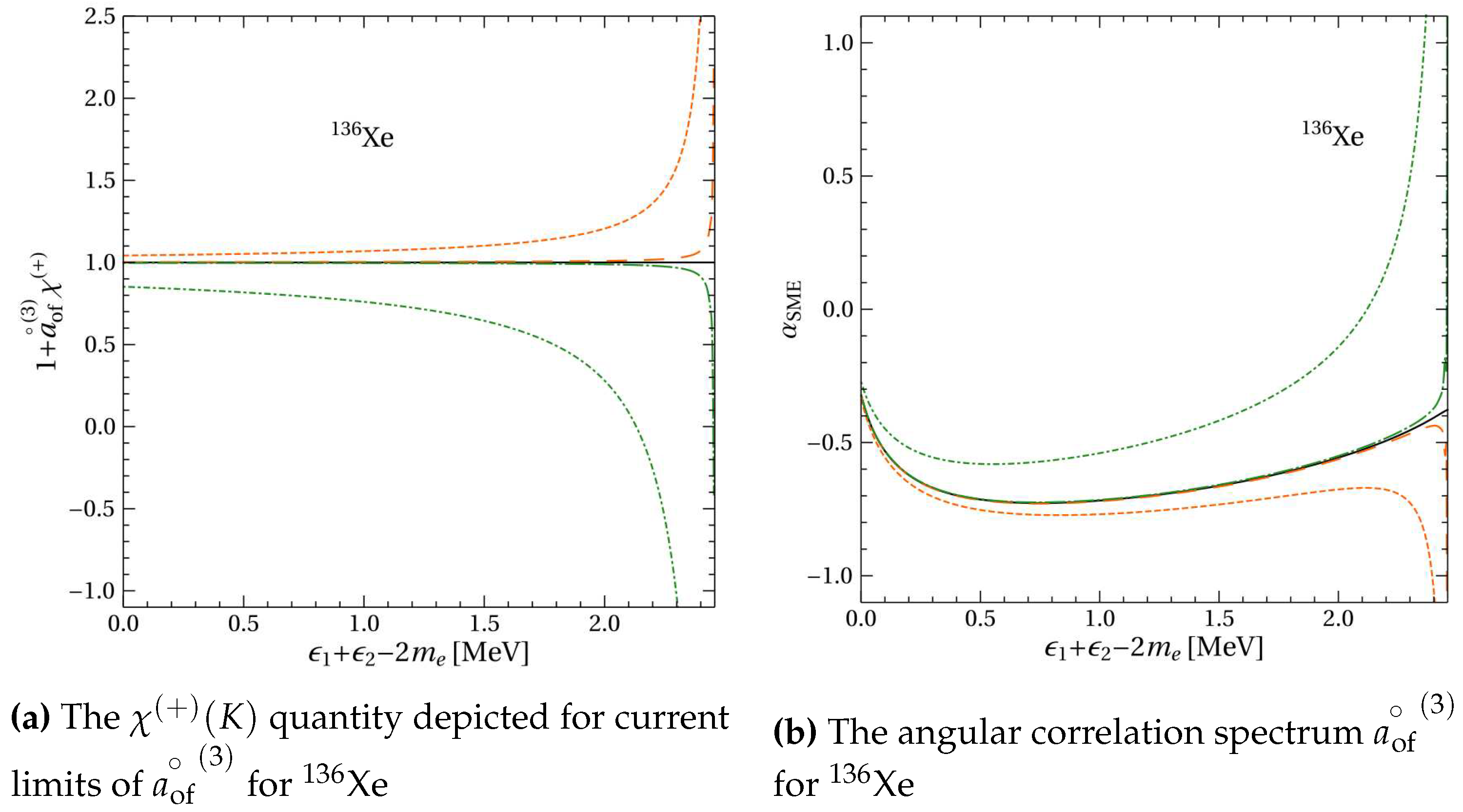

Table 1.
Correlation matrix for 9 observables of Xe from [38].
Table 1.
Correlation matrix for 9 observables of Xe from [38].
| D | D | D | D | P | P | D | |||
| 1 | 0.8 | 0.78 | 0.74 | 0.72 | 0.38 | 0.25 | -0.18 | -0.42 | |
| 0.8 | 1 | 0.47 | 0.43 | 0.42 | 0.52 | 0.44 | -0.049 | -0.24 | |
| D | 0.78 | 0.47 | 1 | 0.95 | 0.96 | 0.53 | 0.34 | -0.54 | -0.79 |
| D | 0.74 | 0.43 | 0.95 | 1 | 0.99 | 0.5 | 0.32 | -0.56 | -0.84 |
| D | 0.72 | 0.42 | 0.96 | 0.99 | 1 | 0.55 | 0.35 | -0.55 | -0.88 |
| D | 0.38 | 0.52 | 0.53 | 0.5 | 0.55 | 1 | 0.76 | -0.23 | -0.58 |
| P | 0.25 | 0.44 | 0.34 | 0.32 | 0.35 | 0.76 | 1 | -0.25 | -0.43 |
| P | -0.18 | -0.049 | -0.54 | -0.56 | -0.55 | -0.23 | -0.25 | 1 | 0.65 |
| D | -0.42 | -0.24 | -0.79 | -0.84 | -0.88 | -0.58 | -0.43 | 0.65 | 1 |
Table 2.
Comparison between several theoretical models results and measured electron capture decay ratios for isotopes studied in [70].
Table 2.
Comparison between several theoretical models results and measured electron capture decay ratios for isotopes studied in [70].
| Isotope | [70] | Quantity | BS[70] | KLI[70] | [68] | RD[71] |
| (keV) | frozen orbitals | |||||
| 1 | ||||||
| 1 | ||||||
| 1 | ||||||
| 1 |
Disclaimer/Publisher’s Note: The statements, opinions and data contained in all publications are solely those of the individual author(s) and contributor(s) and not of MDPI and/or the editor(s). MDPI and/or the editor(s) disclaim responsibility for any injury to people or property resulting from any ideas, methods, instructions or products referred to in the content. |
© 2024 by the authors. Licensee MDPI, Basel, Switzerland. This article is an open access article distributed under the terms and conditions of the Creative Commons Attribution (CC BY) license (http://creativecommons.org/licenses/by/4.0/).
Copyright: This open access article is published under a Creative Commons CC BY 4.0 license, which permit the free download, distribution, and reuse, provided that the author and preprint are cited in any reuse.


