Submitted:
25 January 2024
Posted:
09 February 2024
You are already at the latest version
Abstract
Keywords:
1. Introduction
2. The Research Gap: Naturally Caused Armed Conflict
3. Theory and Hypotheses
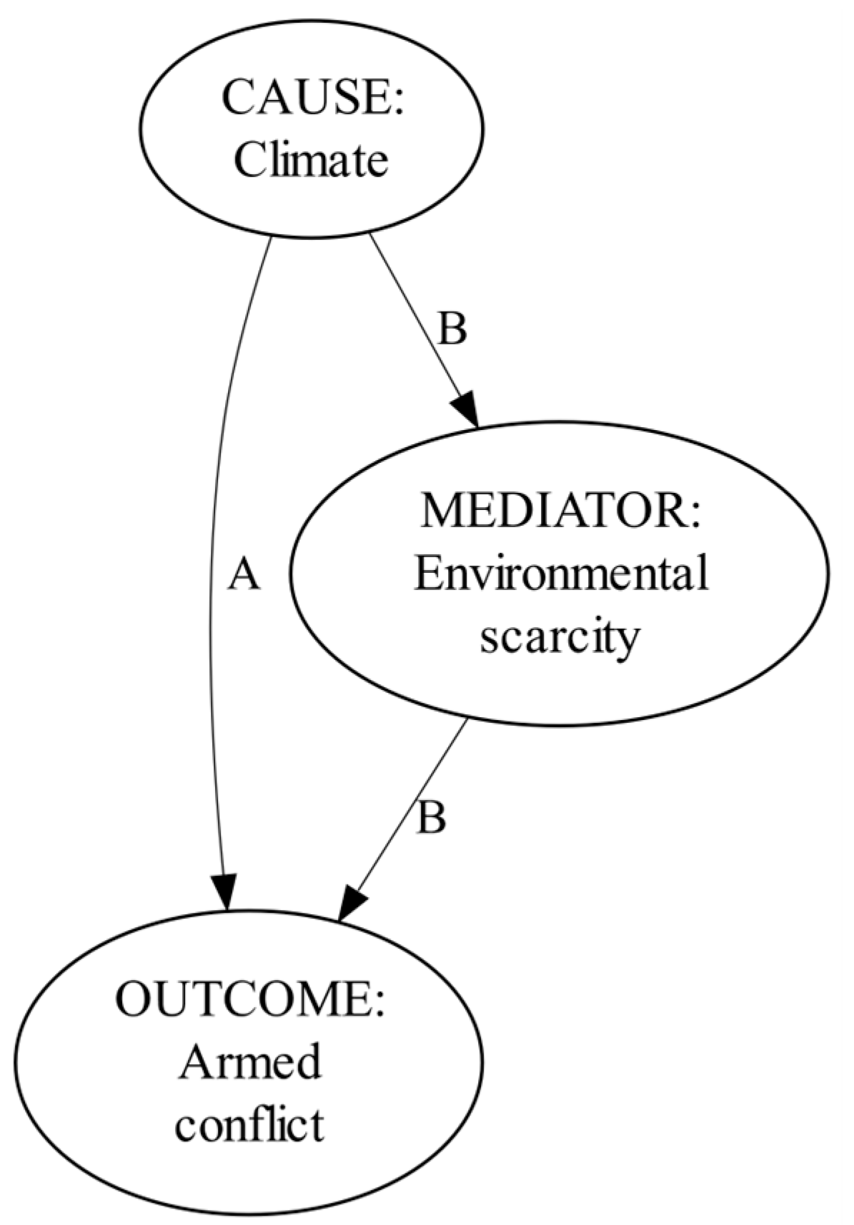
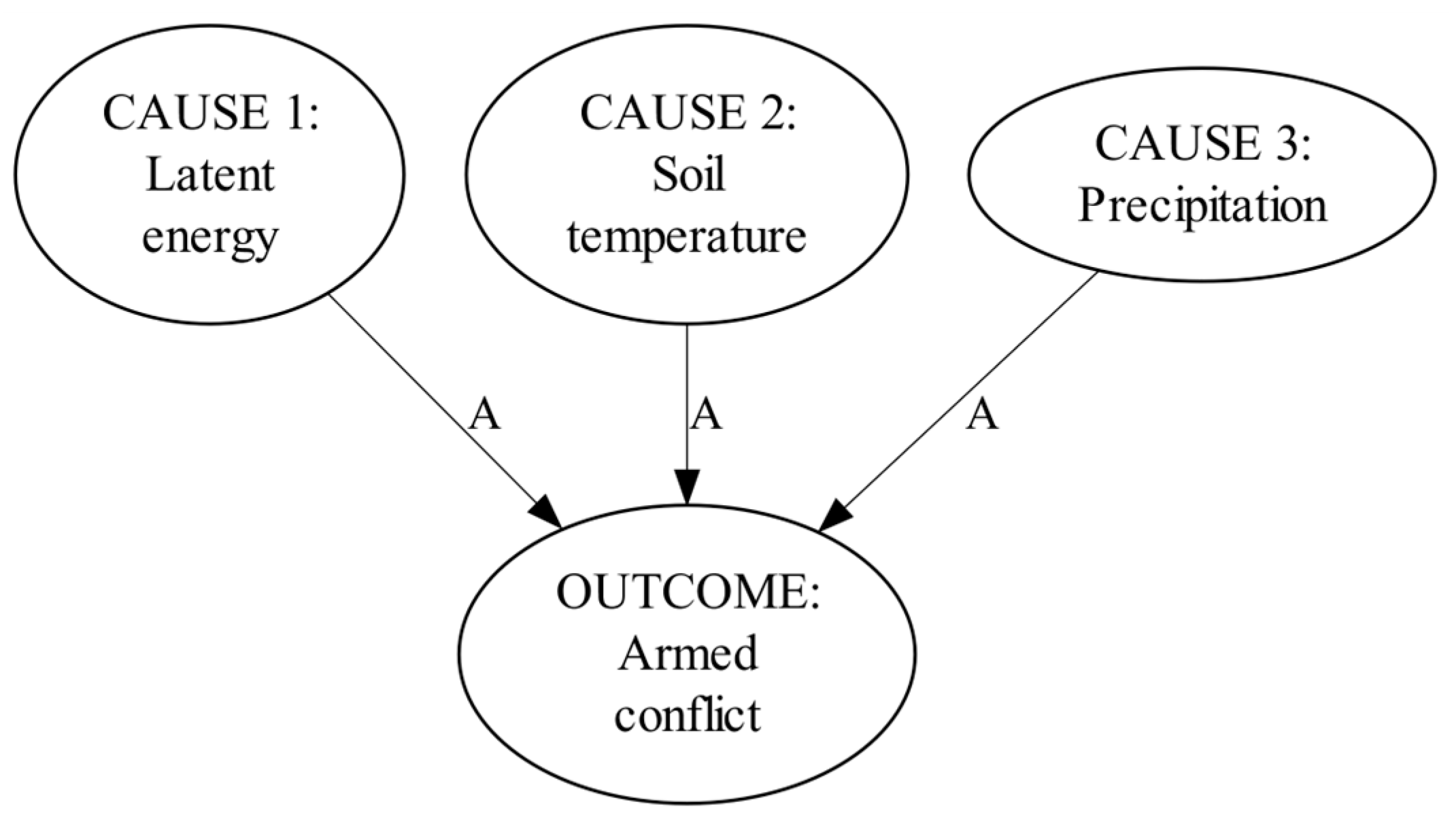
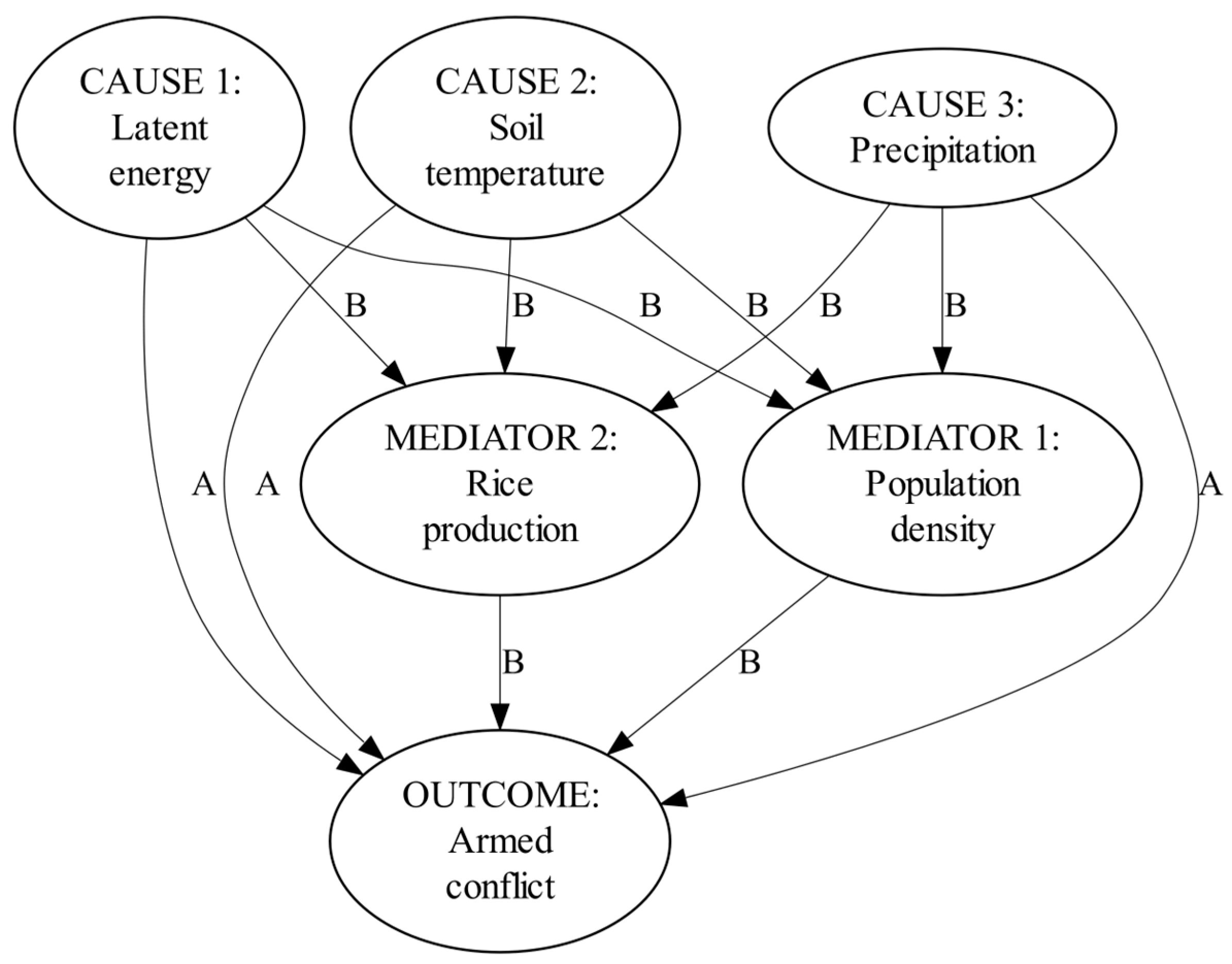
- H1 a): An increase in latent energy in the form of heat directly causes an increase in armed conflict activity.
- H1 b): An increase in soil temperature directly causes an increase in armed conflict activity.
- H1 c): An increase in precipitation (Heat is defined as the energy emanating from the physical surroundings (Glickman and Zenk 2000)) directly causes a decrease in the armed conflict activity.
- H2 a): An increase in latent energy indirectly causes an increase in armed conflict activity.
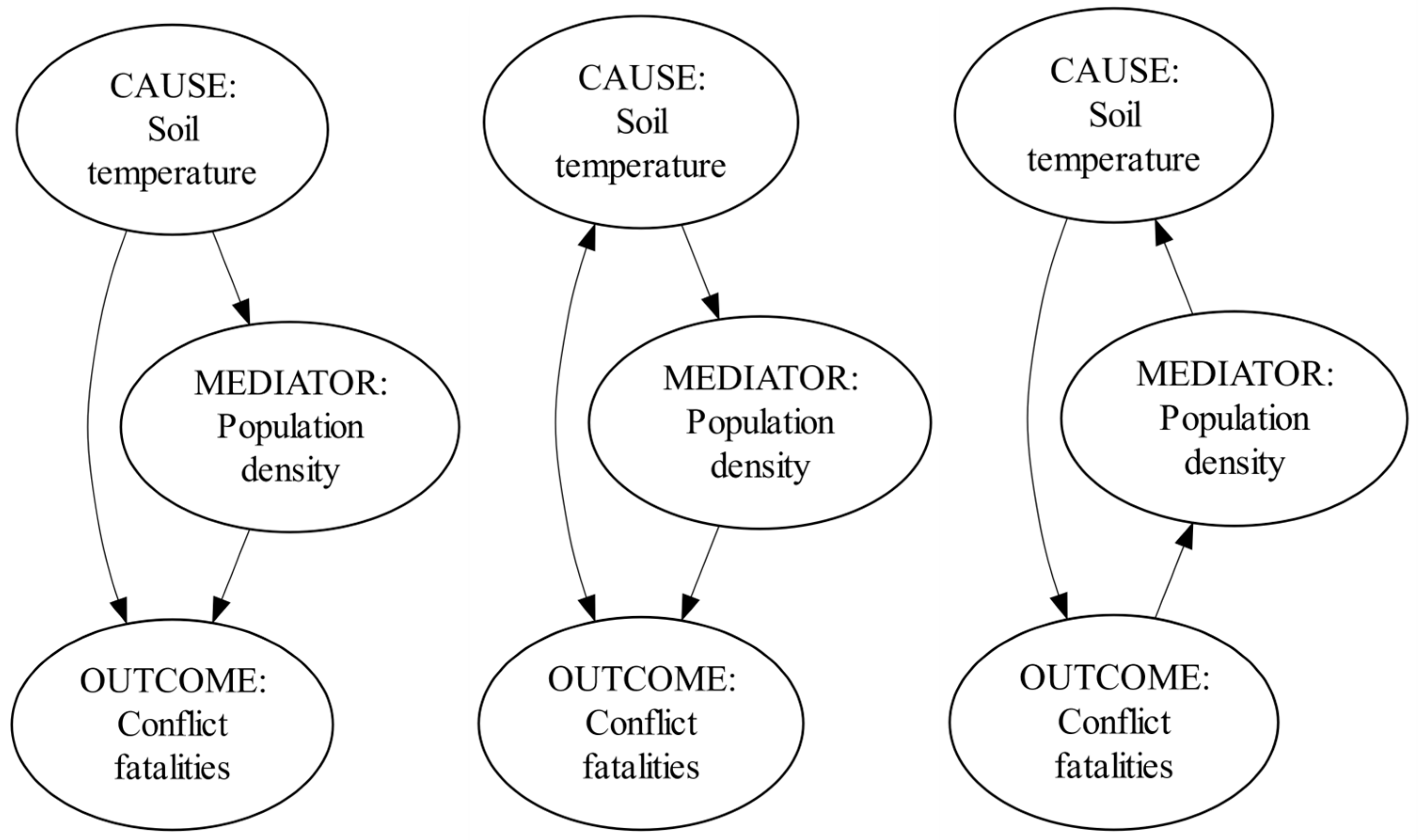
- H2 b): An increase in soil temperature indirectly causes an increase in armed conflict activity.
- H2 c): An increase in precipitation indirectly causes a decrease in armed conflict activity.
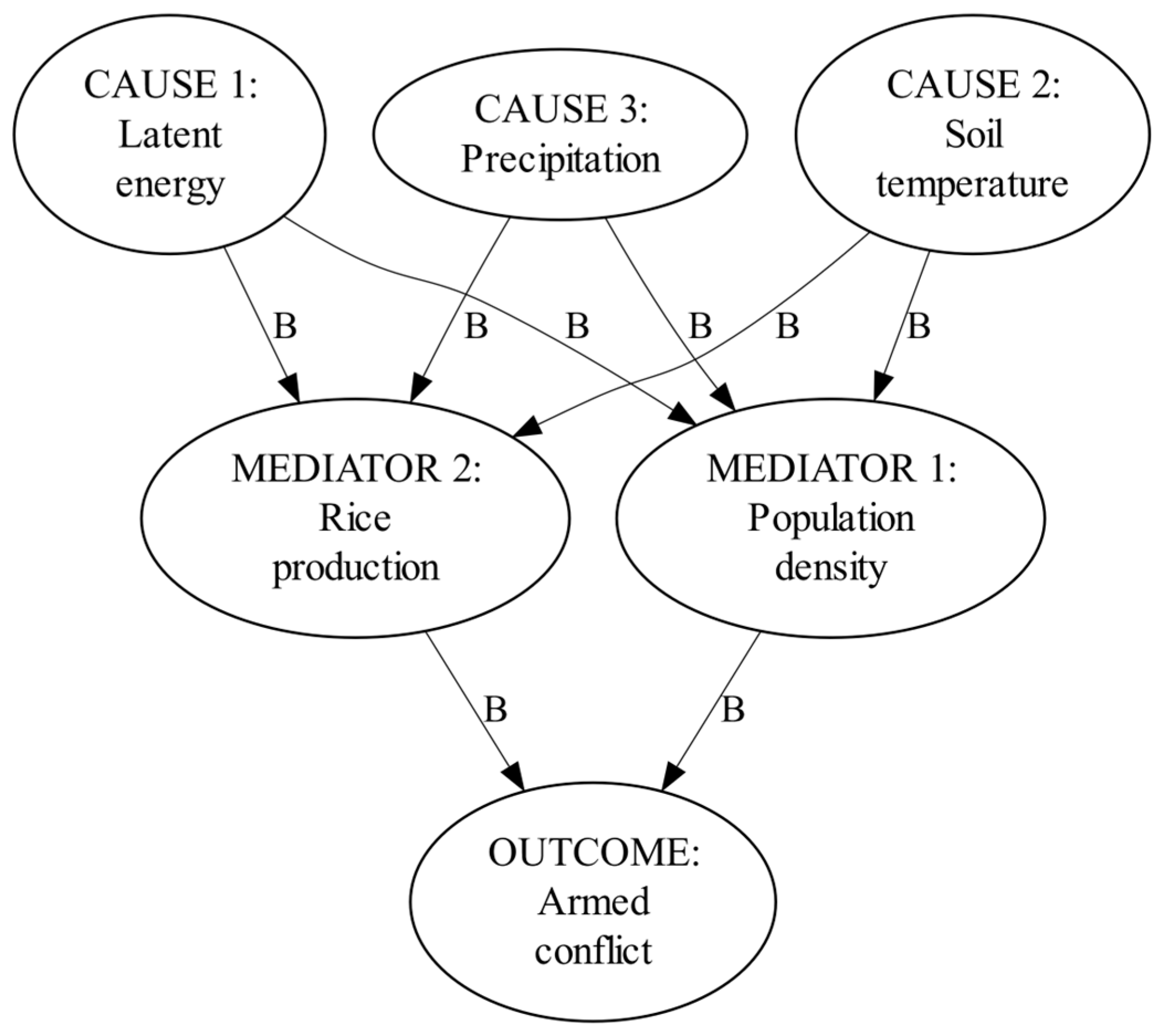
- H3 a): Given the indirect paths from the climatological processes to armed conflict activity, rice production causally mediates the indirect effects of climatological processes on armed conflict activity, by causing an additional decrease in armed conflict activity.
- H3 b): Given the indirect paths from the climatological processes to armed conflict activity, population density causally mediates the indirect effects of climatological processes on armed conflict activity, by causing an additional increase in armed conflict activity.
4. Data and Methods
4.1. Data Sources
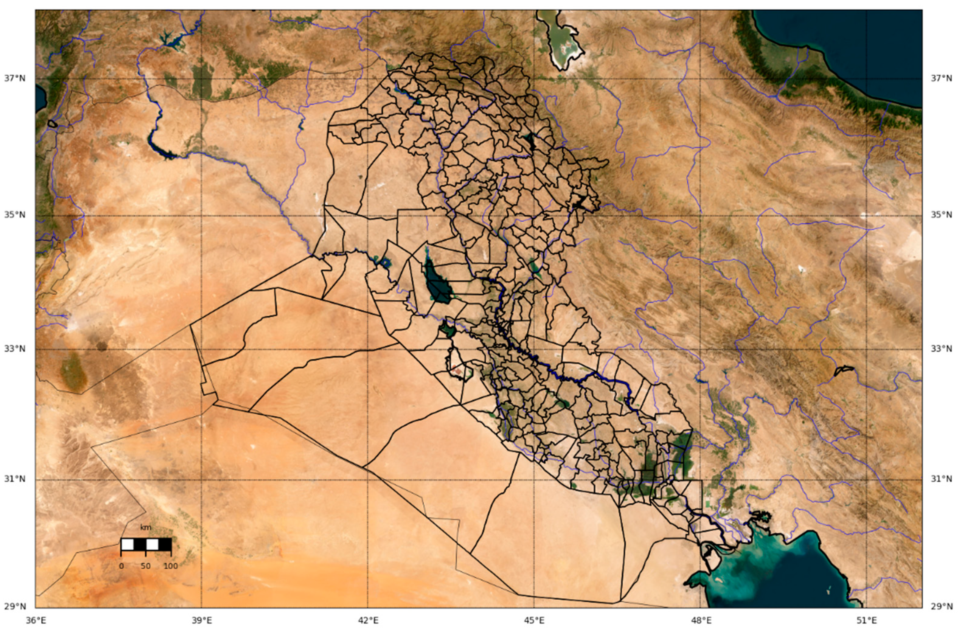
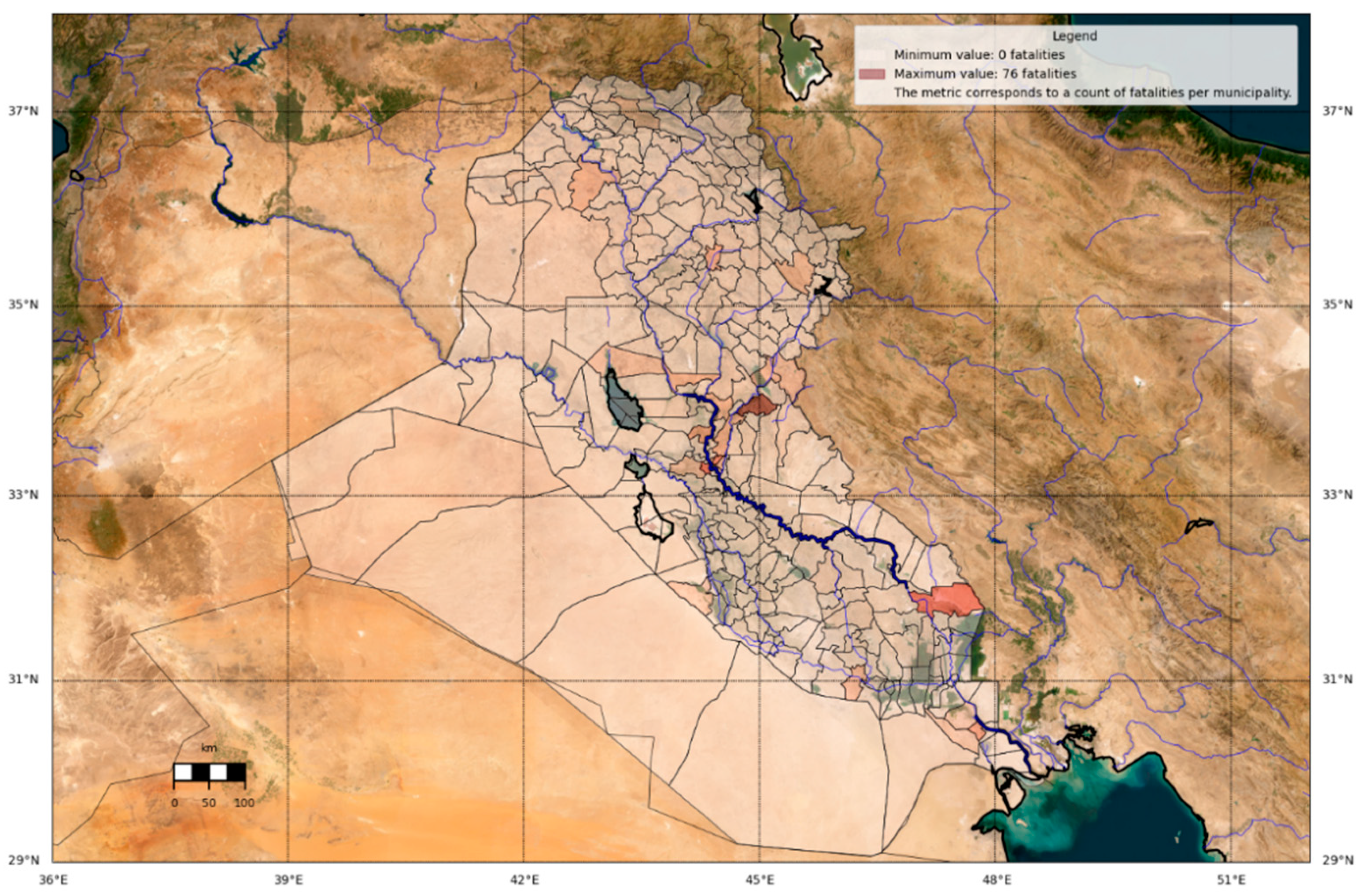
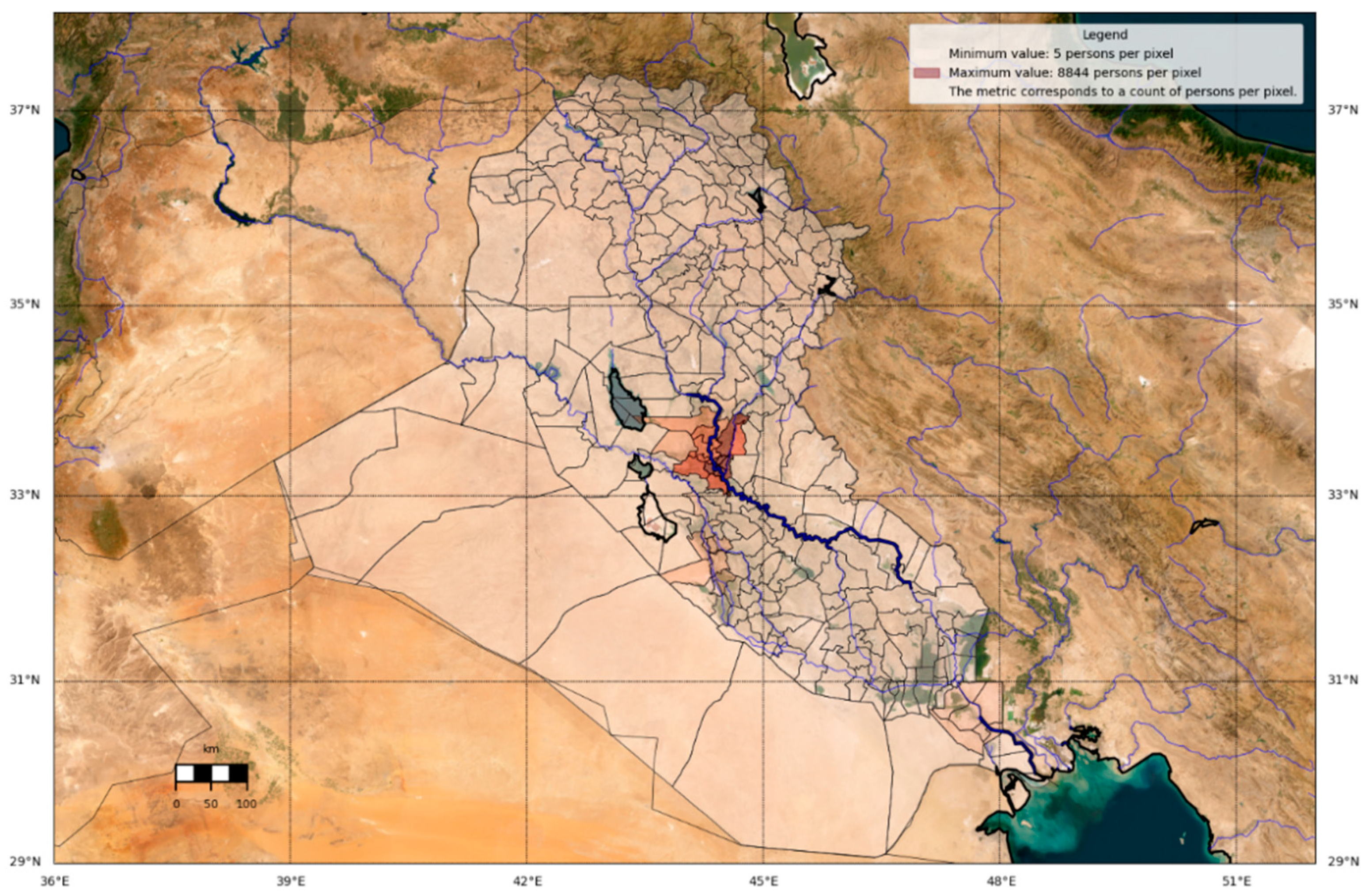
4.2. Methods
| Causal Discovery | Causal Identification | Causal Estimation |
| Retrieval of a causal structure from non-experimental observations. | Verification if a causal query has a unique answer and, if so, formulation of a causal effect as a quantity that is yet to be estimated (i.e., causal estimand). | Calculation of a causal effect as a quantity that has been estimated (i.e., causal estimate), and testing that its probability is not due to randomness. |
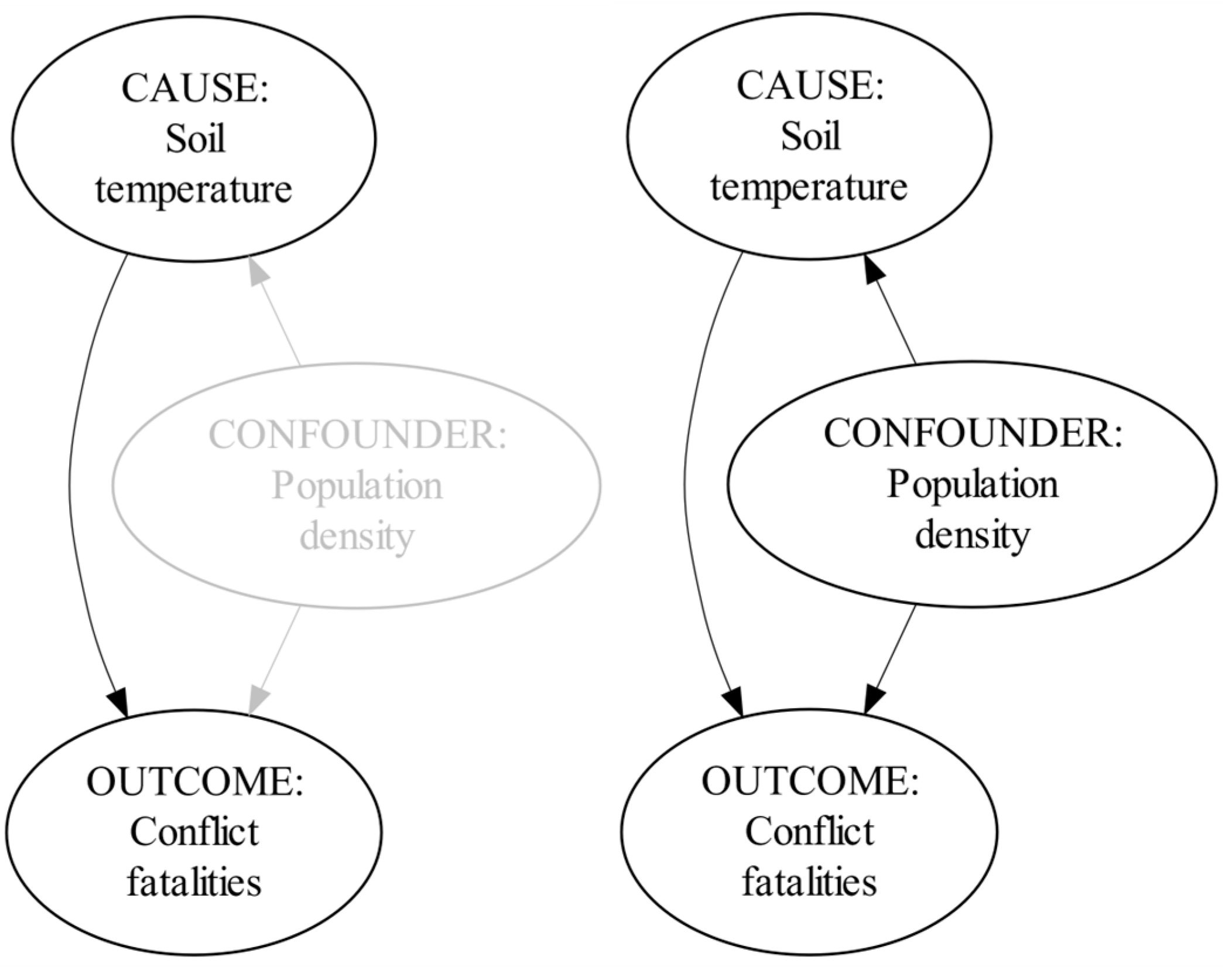
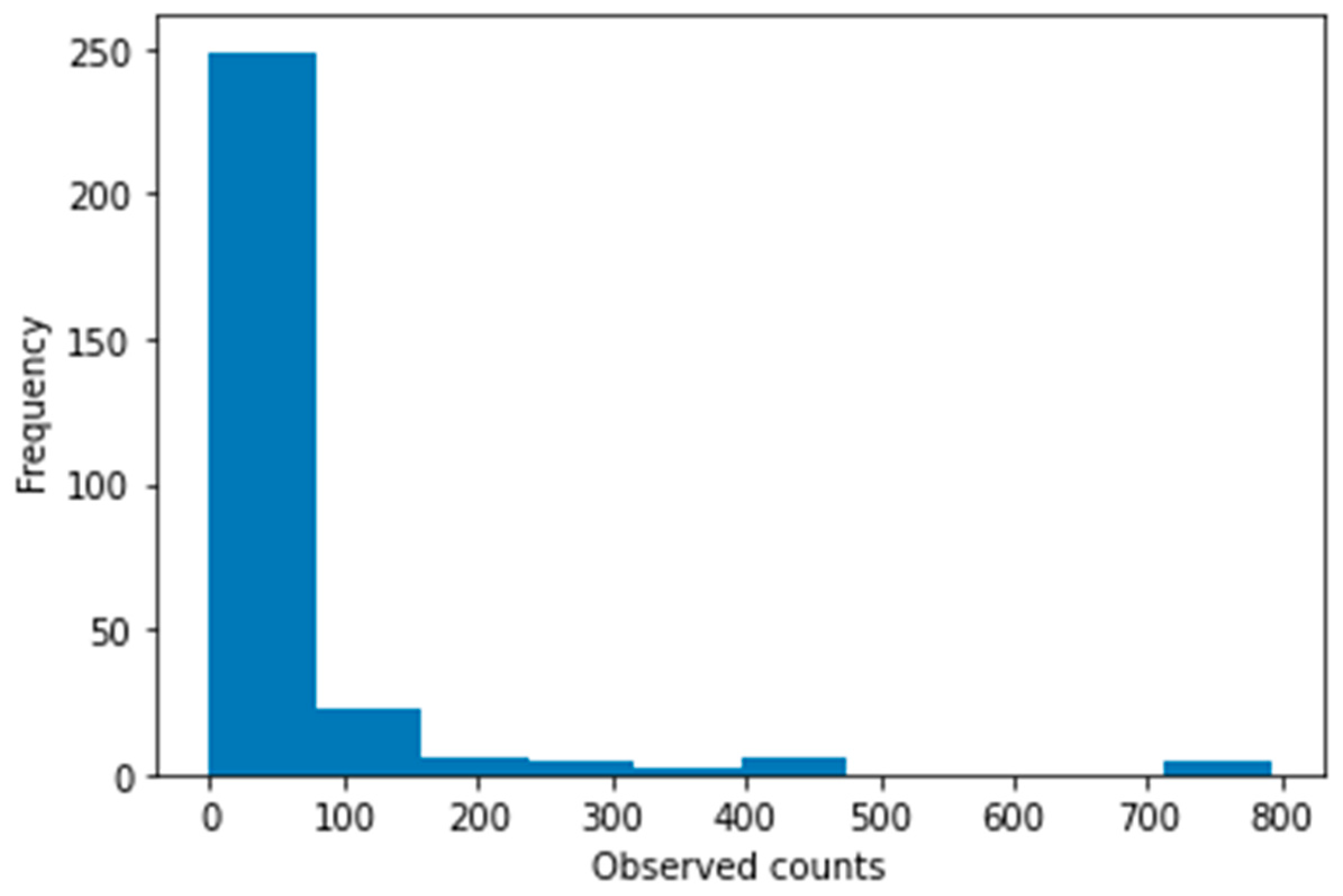
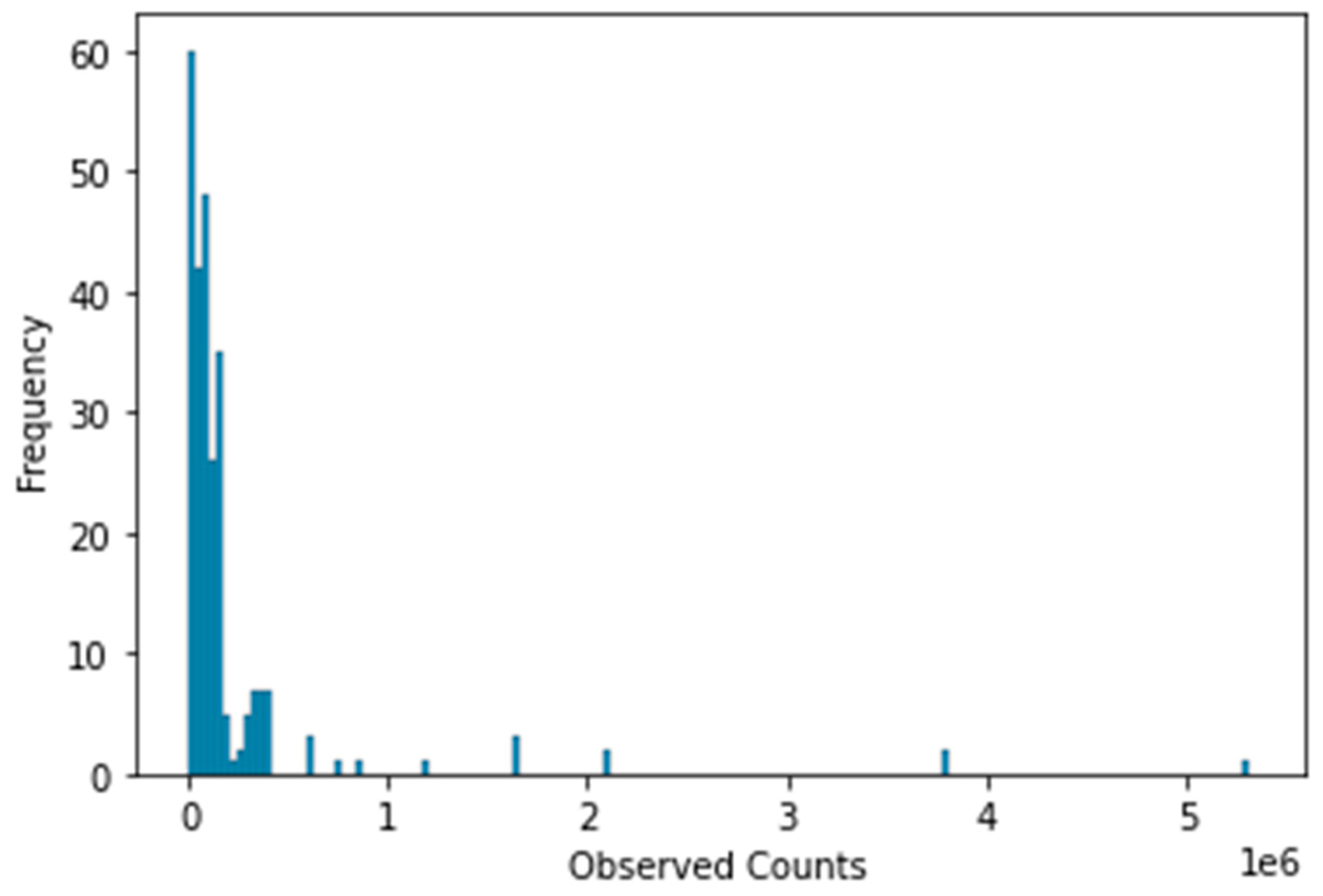
5. Results
Empirical Causal Structure
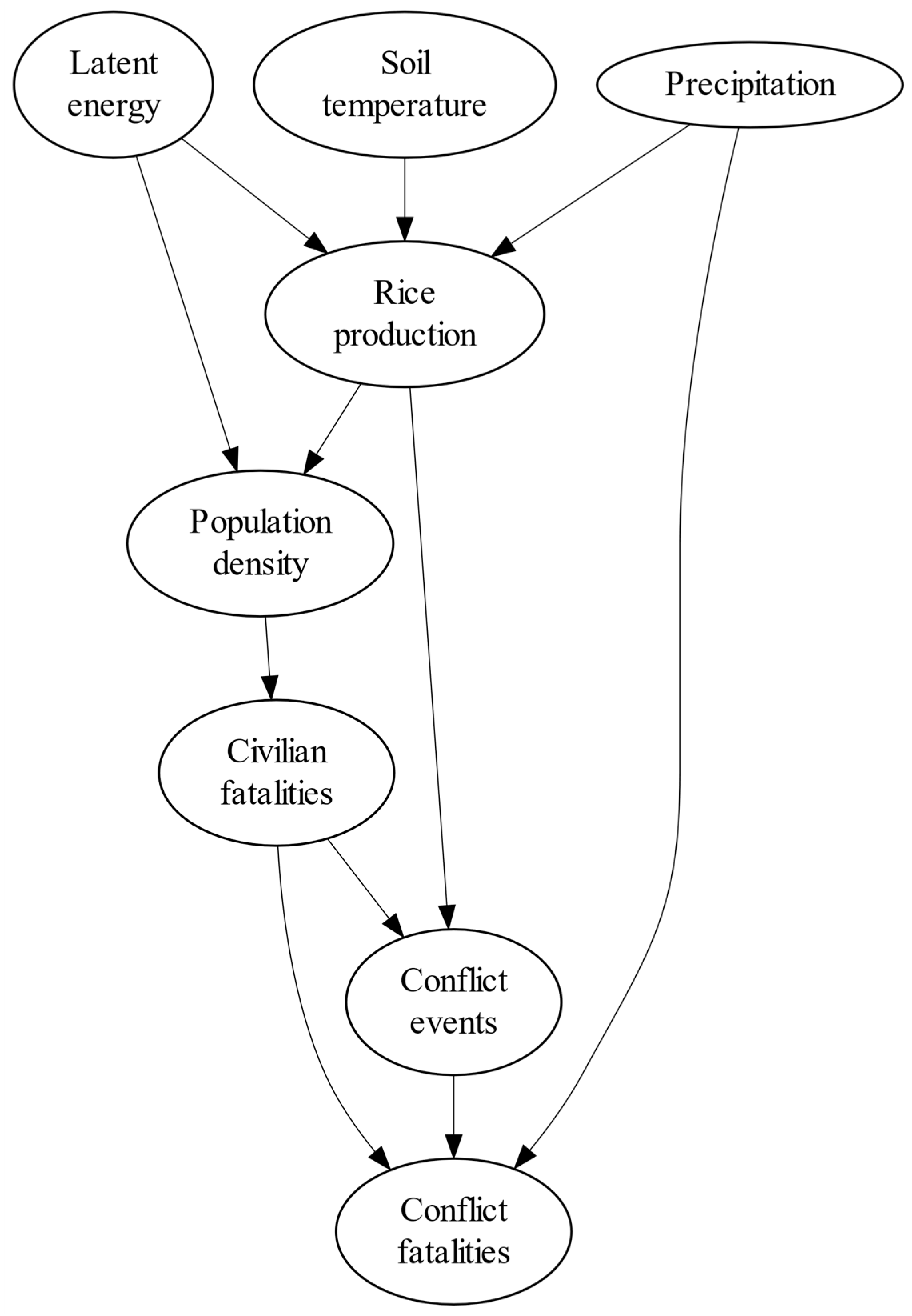
| Causal nodes: | Degree | Degree Centrality |
Betweenness Centrality |
Closeness Centrality |
| Soil Temperature |
1 |
0.125 |
0 |
0 |
| Precipitation | 2 | 0.25 | 0 | 0 |
| Latent energy | 3 | 0.25 | 0 | 0 |
| Rice Production | 5 | 0.625 | 0.152 | 0.375 |
| Population Density | 3 | 0.375 | 0.080 | 0.333 |
| Apart from degree metric which counts the number of edges per node, all the centrality metrics range from 0 to 1. 0 characterizes nodes on the periphery of empirical causal structure, and 1 characterizes the maximum centrality of node for the empirical causal structure. For more on centrality metrics, please refer to Hansen et al. (2020). | ||||
Causal Hypotheses
| Intervention Variables: | |
| Soil Temperature | 1.201e+18*** (8.055e+24) |
| Precipitation | 88.764 (141.988) |
| Latent energy | 506.108* (7.2e+13) |
| Rice Production | -36.417*** (6.827) |
| Population Density | 138.097* (75.33) |
| The table shows standardized causal estimates. The estimation of causal effects was conducted with Generalized Linear Models and Negative-Binomial distribution. Reflecting the uncertainty of estimated causal effects, the corresponding standard errors are in the brackets. Statistical significance level: 5%: *; 1%: **; 0.1%: ***. | |
6. Discussion
6.1. Contributions
6.2. Research Caveats
6.3. Future Directions
6.4. Policy Relevance
7. Conclusion
References
- Abatzoglou, John T., Solomon Z. Dobrowski, Sean A. Parks, and Katherine C. Hegewisch. “TerraClimate, a High-Resolution Global Dataset of Monthly Climate and Climatic Water Balance from 1958–2015.” Scientific Data 5, no. 1 (January 9, 2018). [CrossRef]
- Al-Muqdadi, Sameh W., Mohammed F. Omer, Rudy Abo, and Alice Naghshineh. “Dispute over Water Resource Management—Iraq and Turkey.” Journal of Environmental Protection 07, no. 08 (January 1, 2016): 1096–1103. [CrossRef]
- Acemoglu, Daron, Leopoldo Fergusson, and Simon Johnson. “Population and Conflict.” The Review of Economic Studies 87, no. 4 (August 21, 2019): 1565–1604. [CrossRef]
- Adano, W.R., Ton Dietz, Karen Witsenburg, and Fred Zaal. “Climate Change, Violent Conflict and Local Institutions in Kenya’s Drylands.” Journal of Peace Research 49, no. 1 (January 1, 2012): 65–80. [CrossRef]
- Ash, Konstantin, and Nick Obradovich. “Climatic Stress, Internal Migration, and Syrian Civil War Onset.” Journal of Conflict Resolution 64, no. 1 (July 25, 2019): 3–31. [CrossRef]
- Baechler, Günther. Violence through Environmental Discrimination: Causes, Rwanda Arena, and Conflict Model, 1998. https://ci.nii.ac.jp/ncid/BA47069955.
- Bai, Ying, and James Kai-Sing Kung. “Climate Shocks and Sino-Nomadic Conflict.” The Review of Economics and Statistics 93, no. 3 (August 1, 2011): 970–81. [CrossRef]
- Bergholt, Drago, and Päivi Lujala. “Climate-Related Natural Disasters, Economic Growth, and Armed Civil Conflict.” Journal of Peace Research 49, no. 1 (January 1, 2012): 147–62. [CrossRef]
- Bernauer, Thomas, and Tobias Siegfried. “Climate Change and International Water Conflict in Central Asia.” Journal of Peace Research 49, no. 1 (January 1, 2012): 227–39. [CrossRef]
- Bertsimas, Dimitris, and Omid Nohadani. “Robust Maximum Likelihood Estimation.” Informs Journal on Computing 31, no. 3 (July 1, 2019): 445–58. [CrossRef]
- Bhardwaj, Jessica, Atifa Asghari, Isabella Aitkenhead, Madeleine Jackson, and Yuriy Kuleshov. “Climate Risk and Early Warning Systems: Adaptation Strategies for the Most Vulnerable Communities.” The Journal of Science Policy & Governance 18, no. 02 (June 21, 2021). [CrossRef]
- Bhattacharya, Rohit, Daniel Malinsky, and Ilya Shpitser. “Causal Inference Under Interference And Network Uncertainty.” PubMed 2019 (July 1, 2019). https://pubmed.ncbi.nlm.nih.gov/31885520.
- Bhattacharya, Rohit, Razieh Nabi, and Ilya Shpitser. “Semiparametric Inference For Causal Effects In Graphical Models With Hidden Variables.” ArXiv (Cornell University), March 27, 2020. arXiv:10.48550/arxiv.2003.12659.
- Bhattacharya, Rohit, Tushar Nagarajan, Daniel Malinsky, and Ilya Shpitser. “Differentiable Causal Discovery under Unmeasured Confounding.” ArXiv (Cornell University), March 18, 2021, 2314–22. arXiv:10.48550/arXiv.2010.06978.
- Bollobás, Béla. Random Graphs, 2001. [CrossRef]
- Bongers, Stephan, Patrick Forré, Jonas Peters, and Joris M. Mooij. “Foundations of Structural Causal Models with Cycles and Latent Variables.” Annals of Statistics 49, no. 5 (October 1, 2021). [CrossRef]
- Buhaug, Halvard, Tor A. Benjaminsen, Espen Sjaastad, and Ole Magnus Theisen. “Climate Variability, Food Production Shocks, and Violent Conflict in Sub-Saharan Africa.” Environmental Research Letters 10, no. 12 (December 1, 2015): 125015. [CrossRef]
- Caruso, Raul, Ilaria Petrarca, and Roberto Ricciuti. “Climate Change, Rice Crops and Violence. Evidence from Indonesia.” Social Science Research Network, January 1, 2014. [CrossRef]
- Cederman, Lars-Erik, and Nils B. Weidmann. “Predicting Armed Conflict: Time to Adjust Our Expectations?” Science 355, no. 6324 (February 3, 2017): 474–76. [CrossRef]
- Chadefaux, Thomas. “Conflict Forecasting and Its Limits.” Data Science 1, no. 1–2 (December 8, 2017): 7–17. [CrossRef]
- Couttenier, Mathieu, and Raphael Soubeyran. “Drought and Civil War in Sub-Saharan Africa.” The Economic Journal 124, no. 575 (July 16, 2013): 201–44. [CrossRef]
- Deligiannis, Tom. “The Evolution of Environment-Conflict Research: Toward a Livelihood Framework.” Global Environmental Politics 12, no. 1 (February 1, 2012): 78–100. [CrossRef]
- Dinar, Shlomi, David Katz, Lucia De Stefano, and Brian Blankespoor. “Climate Change, Conflict, and Cooperation: Global Analysis of the Effectiveness of International River Treaties in Addressing Water Variability.” Political Geography 45 (March 1, 2015): 55–66. [CrossRef]
- Fjelde, Hanne, and Nina von Uexkull. “Climate Triggers: Rainfall Anomalies, Vulnerability and Communal Conflict in Sub-Saharan Africa.” Political Geography 31, no. 7 (September 1, 2012): 444–53. [CrossRef]
- Ghimire, Ramesh, and Susana Ferreira. “Floods and Armed Conflict.” Environment and Development Economics 21, no. 1 (June 5, 2015): 23–52. [CrossRef]
- Glickman, Todd, and Walter Zenk. Glossary of Meteorology. American Meteorological Society EBooks, 2000. http://ci.nii.ac.jp/ncid/BA51955944.
- “Gridded Population of the World, Version 4 (GPWV4): Population Density.” Data set, January 1, 2018. https://catalog.data.gov/dataset/gridded-population-of-the-world-version-4-gpwv4-population-density.
- Hansen, Derek L., Ben Shneiderman, Marc A. Smith, and Itai Himelboim. “Calculating and Visualizing Network Metrics.” In Elsevier EBooks, 79–94, 2020. [CrossRef]
- Hayhoe, K. “Climate Change Is a Threat Multiplier.” AGU Fall Meeting Abstracts 2020 (December 1, 2020). http://ui.adsabs.harvard.edu/abs/2020AGUFMSY018..04H/abstract.
- Hegre, Håvard, Joakim Karlsen, Håvard Mokleiv Nygård, Håvard Strand, and Henrik Urdal. “Predicting Armed Conflict, 2010-20501.” International Studies Quarterly 57, no. 2 (December 6, 2012): 250–70. [CrossRef]
- Hegre, Håvard, Håvard Mokleiv Nygård, and Peder Landsverk. “Can We Predict Armed Conflict? How the First 9 Years of Published Forecasts Stand Up to Reality.” International Studies Quarterly 65, no. 3 (January 30, 2021): 660–68. [CrossRef]
- Hendrix, Cullen S., and Sarah M. Glaser. “Trends and Triggers: Climate, Climate Change and Civil Conflict in Sub-Saharan Africa.” Political Geography 26, no. 6 (August 1, 2007): 695–715. [CrossRef]
- Hendrix, Cullen S., and Idean Salehyan. “Climate Change, Rainfall, and Social Conflict in Africa.” Journal of Peace Research 49, no. 1 (January 1, 2012): 35–50. [CrossRef]
- Hilbe, Joseph M. Negative Binomial Regression, 2011. [CrossRef]
- Hitchcock, Christopher, and Judea Pearl. “Causality: Models, Reasoning and Inference.” The Philosophical Review 110, no. 4 (October 1, 2001): 639. [CrossRef]
- Holland, Paul W. “Statistics and Causal Inference.” Journal of the American Statistical Association 81, no. 396 (December 1, 1986): 945–60. [CrossRef]
- Homer-Dixon, Thomas. Environment, Scarcity, and Violence, 2010. [CrossRef]
- ———. “Environmental Scarcities and Violent Conflict: Evidence from Cases.” International Security 19, no. 1 (January 1, 1994): 5. [CrossRef]
- ———. “On the Threshold: Environmental Changes as Causes of Acute Conflict.” International Security 16, no. 2 (January 1, 1991): 76. [CrossRef]
- Homer-Dixon, Thomas, and Jessica Blitt. Ecoviolence : Links among Environment, Population and Security. Rowman & Littlefield EBooks, 1998. http://ci.nii.ac.jp/ncid/BA42666538.
- Hsiang, Solomon, and Marshall Burke. “Climate, Conflict, and Social Stability: What Does the Evidence Say?” Climatic Change 123, no. 1 (October 17, 2013): 39–55. [CrossRef]
- Hsiang, Solomon, Marshall Burke, and Edward Miguel. “Quantifying the Influence of Climate on Human Conflict.” Science 341, no. 6151 (September 13, 2013). [CrossRef]
- Hsiang, Solomon, Kyle C. Meng, and Mark A. Cane. “Civil Conflicts Are Associated with the Global Climate.” Nature 476, no. 7361 (August 1, 2011): 438–41. [CrossRef]
- Hudgens, Michael G., and M. Elizabeth Halloran. “Toward Causal Inference with Interference.” Journal of the American Statistical Association 103, no. 482 (June 1, 2008): 832–42. [CrossRef]
- Huffman, George. IMERG V06 Quality Index, NASA, 2019.
- Huffman, George J., Robert F. Adler, David T. Bolvin, and Eric Nelkin. “The TRMM Multi-Satellite Precipitation Analysis (TMPA).” In Springer EBooks, 3–22, 2009. [CrossRef]
- Ide, Tobias, Miguel Rodriguez Lopez, Christiane Fröhlich, and Jürgen Scheffran. “Pathways to Water Conflict during Drought in the MENA Region.” Journal of Peace Research 58, no. 3 (July 2, 2020): 568–82. [CrossRef]
- International Food Policy Research Institute, 2019, “Global Spatially-Disaggregated Crop Production Statistics Data for 2010 Version 2.0”, Harvard Dataverse, V4. [CrossRef]
- “Inventing Temperature: Measurement and Scientific Progress.” Choice Reviews Online 43, no. 01 (September 1, 2005): 43–0373. [CrossRef]
- Koren, Ore. “Food Resources and Strategic Conflict.” Journal of Conflict Resolution 63, no. 10 (March 11, 2019): 2236–61. [CrossRef]
- Koubi, Vally. “Climate Change and Conflict.” Annual Review of Political Science 22, no. 1 (May 11, 2019): 343–60. [CrossRef]
- Koubi, Vally, Thomas Bernauer, Anna Kalbhenn, and Gabriele Spilker. “Climate Variability, Economic Growth, and Civil Conflict.” Journal of Peace Research 49, no. 1 (January 1, 2012): 113–27. [CrossRef]
- Kress, Moshe. “Modeling Armed Conflicts.” Science 336, no. 6083 (May 18, 2012): 865–69. [CrossRef]
- Lee, Jaron J. R., Rohit Bhattacharya, Razieh Nabi, and Ilya Shpitser. “Ananke: A Python Package For Causal Inference Using Graphical Models.” ArXiv (Cornell University), January 26, 2023. arXiv:10.48550/arxiv.2301.11477.
- Lundberg, Ian, Rebecca A. Johnson, and Brandon Stewart. “What Is Your Estimand? Defining the Target Quantity Connects Statistical Evidence to Theory.” American Sociological Review 86, no. 3 (June 1, 2021): 532–65. [CrossRef]
- Mach, Katharine J., Caroline M. Kraan, W. Neil Adger, Halvard Buhaug, Marshall Burke, James D. Fearon, Christopher B. Field, et al. “Climate as a Risk Factor for Armed Conflict.” Nature 571, no. 7764 (June 12, 2019): 193–97. [CrossRef]
- Malinsky, Daniel, and David Danks. “Causal Discovery Algorithms: A Practical Guide.” Philosophy Compass 13, no. 1 (November 23, 2017): e12470. [CrossRef]
- McNally, Amy, Kristi R. Arsenault, Sujay V. Kumar, Shraddhanand Shukla, Peter Y. Peterson, Shugong Wang, Chris Funk, Christa D. Peters-Lidard, and J. P. Verdin. “A Land Data Assimilation System for Sub-Saharan Africa Food and Water Security Applications.” Scientific Data 4, no. 1 (February 14, 2017). [CrossRef]
- Muñoz-Sabater, Joaquín, Emanuel Dutra, Anna Agusti-Panareda, Clément Albergel, Gabriele Arduini, Gianpaolo Balsamo, Souhail Boussetta, et al. “ERA5-Land: A State-of-the-Art Global Reanalysis Dataset for Land Applications.” Earth System Science Data 13, no. 9 (September 7, 2021): 4349–83. [CrossRef]
- Nichols, Austin. “Causal Inference with Observational Data.” Stata Journal 7, no. 4 (December 1, 2007): 507–41. [CrossRef]
- Pearl, Judea. “Causal Inference in Statistics: An Overview.” Statistics Surveys 3, no. none (January 1, 2009). [CrossRef]
- ———. “The Do-Calculus Revisited.” ArXiv (Cornell University), October 16, 2012. arXiv:10.48550/arxiv.1210.4852.
- Raleigh, Clionadh. “Political Marginalization, Climate Change, and Conflict in African Sahel States.” International Studies Review 12, no. 1 (March 1, 2010): 69–86. [CrossRef]
- Raleigh, Clionadh, and Håvard Hegre. “Population Size, Concentration, and Civil War. A Geographically Disaggregated Analysis.” Political Geography 28, no. 4 (May 1, 2009): 224–38. [CrossRef]
- Raleigh, Clionadh, Andrew M. Linke, Håvard Hegre, and Joakim Karlsen. “Introducing ACLED: An Armed Conflict Location and Event Dataset.” Journal of Peace Research 47, no. 5 (September 1, 2010): 651–60. [CrossRef]
- Reuveny, Rafael. “Climate Change-Induced Migration and Violent Conflict.” Political Geography 26, no. 6 (August 1, 2007): 656–73. [CrossRef]
- Robins, James M. “A New Approach to Causal Inference in Mortality Studies with a Sustained Exposure Period—Application to Control of the Healthy Worker Survivor Effect.” Mathematical Modelling 7, no. 9–12 (January 1, 1986): 1393–1512. [CrossRef]
- Rodríguez-Labajos, Beatriz, and Joan Martinez-Alier. “Political Ecology of Water Conflicts.” Wiley Interdisciplinary Reviews: Water 2, no. 5 (June 3, 2015): 537–58. [CrossRef]
- Rubin, Donald B. “Bayesian Inference for Causal Effects: The Role of Randomization.” Annals of Statistics 6, no. 1 (January 1, 1978). [CrossRef]
- ———. “Causal Inference Using Potential Outcomes.” Journal of the American Statistical Association 100, no. 469 (March 1, 2005): 322–31. [CrossRef]
- ———. “Estimating Causal Effects of Treatments in Randomized and Nonrandomized Studies.” Journal of Educational Psychology 66, no. 5 (October 1, 1974): 688–701. [CrossRef]
- Runge, Jakob, Peer Nowack, Marlene Kretschmer, Seth Flaxman, and Dino Sejdinovic. “Detecting and Quantifying Causal Associations in Large Nonlinear Time Series Datasets.” Science Advances 5, no. 11 (November 1, 2019). [CrossRef]
- Running, Steve, Mu Qiaozhen. MOD16A2 MODIS/Terra Evapotranspiration 8-day L4 Global 500m SIN Grid. NASA LP DAAC. - University of Montana and MODAPS SIPS - NASA. (2015). http://doi.org/10.5067/MODIS/MOD16A2.006.
- Sagi, Omer, and Lior Rokach. “Explainable Decision Forest: Transforming a Decision Forest into an Interpretable Tree.” Information Fusion 61 (September 1, 2020): 124–38. [CrossRef]
- Sakaguchi, Kendra, Anil Varughese, and Graeme Auld. “Climate Wars? A Systematic Review of Empirical Analyses on the Links between Climate Change and Violent Conflict.” International Studies Review 19, no. 4 (October 5, 2017): 622–45. [CrossRef]
- Shpitser Ilya, and Judea Pearl. “Complete Identification Methods for the Causal Hierarchy.” Journal of Machine Learning Research, June 1, 2008. [CrossRef]
- Slettebak, Rune. “Don’t Blame the Weather! Climate-Related Natural Disasters and Civil Conflict.” Journal of Peace Research 49, no. 1 (January 1, 2012): 163–76. [CrossRef]
- Spirtes, Peter, Clark Glymour, and Richard Scheines. Causation, Prediction, and Search. Lecture Notes in Statistics, 1993. [CrossRef]
- Sundberg, Ralph, and Erik Melander. “Introducing the UCDP Georeferenced Event Dataset.” Journal of Peace Research 50, no. 4 (July 1, 2013): 523–32. [CrossRef]
- Suzuki, Susumu, Volker Krause, and J. David Singer. “The Correlates of War Project: A Bibliographic History of the Scientific Study of War and Peace, 1964-2000.” Conflict Management and Peace Science 19, no. 2 (September 1, 2002): 69–107. [CrossRef]
- Sweijs, Tim, Marlijn de Haan, Hugo van Manen. Unpacking the Climate Security Nexus Seven Pathologies Linking Climate Change to Violent Conflict, The Hague: The Hague Centre for Strategic Studies, 2022.
- Tian, Jin, and Judea Pearl. “A General Identification Condition for Causal Effects.” National Conference on Artificial Intelligence, July 28, 2002, 567–73. [CrossRef]
- Tir, Jaroslav, and Paul F. Diehl. “Demographic Pressure and Interstate Conflict: Linking Population Growth and Density to Militarized Disputes and Wars, 1930-89.” Journal of Peace Research 35, no. 3 (May 1, 1998): 319–39. [CrossRef]
- Urdal, Henrik. “People vs. Malthus: Population Pressure, Environmental Degradation, and Armed Conflict Revisited.” Journal of Peace Research 42, no. 4 (July 1, 2005): 417–34. [CrossRef]
- Ward, Michael D. “Can We Predict Politics? Toward What End?: Table 1.” Journal of Global Security Studies 1, no. 1 (February 1, 2016): 80–91. [CrossRef]
- Wills, Peter R., and François G. Meyer. “Metrics for Graph Comparison: A Practitioner’s Guide.” PLOS ONE 15, no. 2 (February 12, 2020): e0228728. [CrossRef]
- Wolfson, Murray, Anil Puri, and Mario Martelli. “The Nonlinear Dynamics of International Conflict.” Journal of Conflict Resolution 36, no. 1 (March 1, 1992): 119–49. [CrossRef]
- Xiao, Li-Ye, Xiaodong Fang, and Y. Ye. “Reclamation and Revolt: Social Responses in Eastern Inner Mongolia to Flood/Drought-Induced Refugees from the North China Plain 1644–1911.” Journal of Arid Environments 88 (January 1, 2013): 9–16. [CrossRef]
- Yin, Weiwen. “Climate Shocks, Political Institutions, and Nomadic Invasions in Early Modern East Asia.” Journal of Conflict Resolution 64, no. 6 (December 12, 2019): 1043–69. [CrossRef]
- Yoffe, Shira, Aaron T. Wolf, and Mark Giordano. “Conflict and Cooperation over International Freshwater Resources: Indicators of Basins at Risk.” Journal of the American Water Resources Association 39, no. 5 (October 1, 2003): 1109–26. [CrossRef]
Disclaimer/Publisher’s Note: The statements, opinions and data contained in all publications are solely those of the individual author(s) and contributor(s) and not of MDPI and/or the editor(s). MDPI and/or the editor(s) disclaim responsibility for any injury to people or property resulting from any ideas, methods, instructions or products referred to in the content. |
© 2024 by the authors. Licensee MDPI, Basel, Switzerland. This article is an open access article distributed under the terms and conditions of the Creative Commons Attribution (CC BY) license (https://creativecommons.org/licenses/by/4.0/).


