1. Introduction
Strong evidence for the universe’s accelerated expansion is provided by several current standard observations, e.g. type Ia Supernovae (SNeIa), the cosmic microwave background (CMB) radiation, large scale structure (LSS), the Planck satellite, baryon acoustic oscillations (BAO) and the Wilkinson microwave anisotropy probe (WMAP). It is observed that modified gravity could provide a more accurate description of the universe’s accelerating expansion. As far as we are aware, modified gravity offers a straightforward gravitational substitute for the dark energy paradigm. These theories of dark energy are based on expanding the Einstein-Hilbert action with gravitational components. This has the effect of altering the universe’s evolution, either early or late. In modified gravity, there are numerous examples of these models in the literature [
1,
2,
3]. The universe expanded at an incredibly fast rate during the inflationary phase. The discovery of the inflationary era in the late 1970s and early 1980s helped to resolve some of the Big Bang model’s issues. Cosmological models that bounce could be a valid explanation for the universe at both early and late times, according to evidence. A uniform description of this could be provided by modified gravity. A phantom fluid or field is needed to explain the accelerated expansion in standard general relativity. Ultimately, this phantom field results in a large rupture or a singularity of the crushing kind [
4].
Modified gravity is another explanation for the universe’s late-time acceleration. In the initial phase
gravity has been exploited with
R in the Einstein-Hilbert action which is the scalar curvature. This notion is easy to understand, workable and very effective. However, at present General Relativity (GR) has numerous variations. As a result we obtain
theory if the Lagrangian is a function of both
R and the energy-momentum tensor’s trace
T [
5,
6,
7,
8,
9,
10,
11,
12,
13,
14,
15,
16,
17,
18,
19,
20,
21,
22,
23,
24,
25,
26,
27]. In this gravity theory, some of the basic aspects are as follows: (i) here the trace of the energy-momentum tensor
T and (ii) the Ricci scalar
R which have considerable intrinsic features to the matter Lagrangian. Moreover, the quantum field effect as well as the particle creation potentiality are some other attributes to
gravity. All these aspects of modified gravity theories are available in the following review work [
28]. In order to account for heat conduction, viscosity, and quantum effects, the
T term is introduced. There is another explanation for the late time cosmic acceleration. Observational restrictions have been applied to
gravity. However,
gravity presents an intriguing substitute for
gravity and
G referes to the Gauss-Bonnet invariant. Numerous studies in the literature demonstrate that inflation and late-time acceleration can be explained by
gravity [
29,
30,
31,
32,
33,
34,
35,
36,
37,
38,
39,
40,
41,
42]. Here, the analysis of the universe’s physical properties in
gravity is our primary goal.
Understanding of the late-time acceleration of the universe is largely dependent on the mainstream cosmological model. However, a wide variety of models explaining the primary characteristics of the cosmos may be found in the literature. Age, horizon, and fuzziness issues in the standard model are successfully resolved by models based on a power-law of the scale factor [
43,
44,
45,
46]. In general the expansion rate of the universe is described by the Hubble constant
. In the recent past, we have observed the statistically significant tensions in
which refers to the difference between its direct local distance ladder measurements and consideration of the standard
CDM model. For example there is approximately 4.4
tension in value of
determined by SH0ES measurement
(68% CL) [
47] and
(68% CL) [
48]. This discrepancy in the value of
is referred as
tension. Some important researches on
tension are given in Refs. [
49,
50,
51,
52,
53,
54,
55,
56,
57,
58,
59,
60,
61].
In view of the above mentioned motivation, the plan of the present study is outlined as: in
Section 2, a brief mathematical overview of the metric and
gravity theory along with the solution to the field equations have been provided. In
Section 3, observational analysis has been executed within the observational constraints of the model parameters. The physical parameters involved in the model are presented by the help of plots in
Section 4. At last,
Section 5 is designed for relevant comments on the entire investigation.
2. The Action and Cosmological Solutions
2.1. Field Equations
In four-dimensional space-time, the modified Gauss-Bonnet gravity operates as
where
and
is the matter Lagrangian which depends upon
and matter fields. The Gauss-Bonnet invariant
G is defined as
. The Gauss-Bonnet invariant is obtained from
,
and
.
From Eq. (
1), the gravitational field equations are derived as
where
is the energy momentum tensor arising from
.
The flat FLRW space-time metric is
where the symbols have their usual meanings.
Now, we calculate the Einstien field equations using Eqs.
2 and
1 as
where
is the Hubble parameter and
.
In the present model, we are taking and this term denotes the difference with general relativity. Here is an arbitrary positive constant.
2.2. Power law cosmology
To implement the power-law based cosmological model, we take the scale factor [
62] as
where
represents the current value of the scale factor and
is a dimensionless parameter.
Now, the scale factor may be used to characterise the Hubble parameter as
Additionally, the scale factor can be provided via the redshift as
, where
H takes the following form in terms of
z:
We take into account cosmological characteristics like the pressure, the energy density, the EOS parameter, the Hubble parameter, the deceleration parameter, etc. to comprehend the history of the universe. A dimensionless variable known as the deceleration parameter may be used to calculate the universe’s acceleration or deceleration phase. The definition of the deceleration parameter
q is
Now, the following three cases may arise: (i) if
, then the phase of the universe is decelerating, (ii) if
, it is accelerating and (iii) if
, it is expanding continuously. As a result, Eqs. (
8) – (
12) provide
So, using the deceleration parameter
q and redshift, we can describe the Hubble parameter as follows
Let us now get the expressions for the energy density and the pressure by solving Eqs. (
4) and (
5), which are given as
We accept and as unity for further analysis, and we limit and q using three current observational data sets: , BAO and Pantheon compilation of SN Ia data.
3. Observational Constraints on Model Parameters
In this section, observational data sets are utilised to restrict the values of
and
q that occur in the tilted Hubble parametrization. In this model, we employ the
, BAO, and Pantheon data sets, as well as their combined data collections. The
data points are given in [
63]. The information on BAO and Pantheon compilation of SN Ia data are sourced from [
64] and [
65,
66,
67,
68] respectively.
3.1. Observed Hubble Data (OHD) set
We utilise the 57-point OHD data from [
63]. The best-fit values of
and
q are now found using the standard chi-square test. The Chi-square is calculated as follows
where
and
are respectively the observed and theoretical values and
is the standard deviation at
.
3.2. BAO Data set
Let us utilize BAO data to evaluate and verify the probable predictions of our cosmological models at various redshift values. This will obviously offer a unique method to examine the expansion parameters of the presently accelerating universe at low redshift values. Here the BAO dataset has been obtained from the current surveys, e.g. 6dFGS, SDSS and WiggleZ, spanning in the specific redshift range
. The basic idea behind this is as follows: the dimensionless amount serves to obtain a clear-cut indication of the primordial baryon-photon acoustic oscillations in the matter power spectrum. Hence
3.3. Pantheon Data set
For the redshift range of
, we utilise the Pantheon data compilation, which has 1048 data points. This data is taken from different supernovae survey, e.g. In the range of
,
,
,
,
, and
respectively, C
fA1 - 4, CSP, SDSS, SNLS, PS1, high
z gives 147, 25, 335, 236, 279, 26 SN Ia for each Sample. The investigation of the expansion rate heavily relies on SNeIa. To assess the theoretically expected apparent magnitude (m) and absolute magnitude (
M) with respect to colour and stretch, we thus compute the distance modulus
as follows
where
and
are respectively the luminosity distance and the nuisance parameter.
These are given by
respectively.
Now, the minimum
function is given as
3.4. Joint OHD + Pantheon Data set
By performing joint statistical analysis using
and Pantheon data sets, we obtain stronger constraints. Therefore, the chi-sq function for joint data sets can be written as
3.5. Joint OHD + BAO + Pantheon Data set
By performing joint statistical analysis using
, BAO and Pantheon data sets, we obtain even stronger and more reliable constraints. Therefore, the chi-sq function for joint data sets can be written as
4. Results under the gravity model
4.1. Parameter Estimation
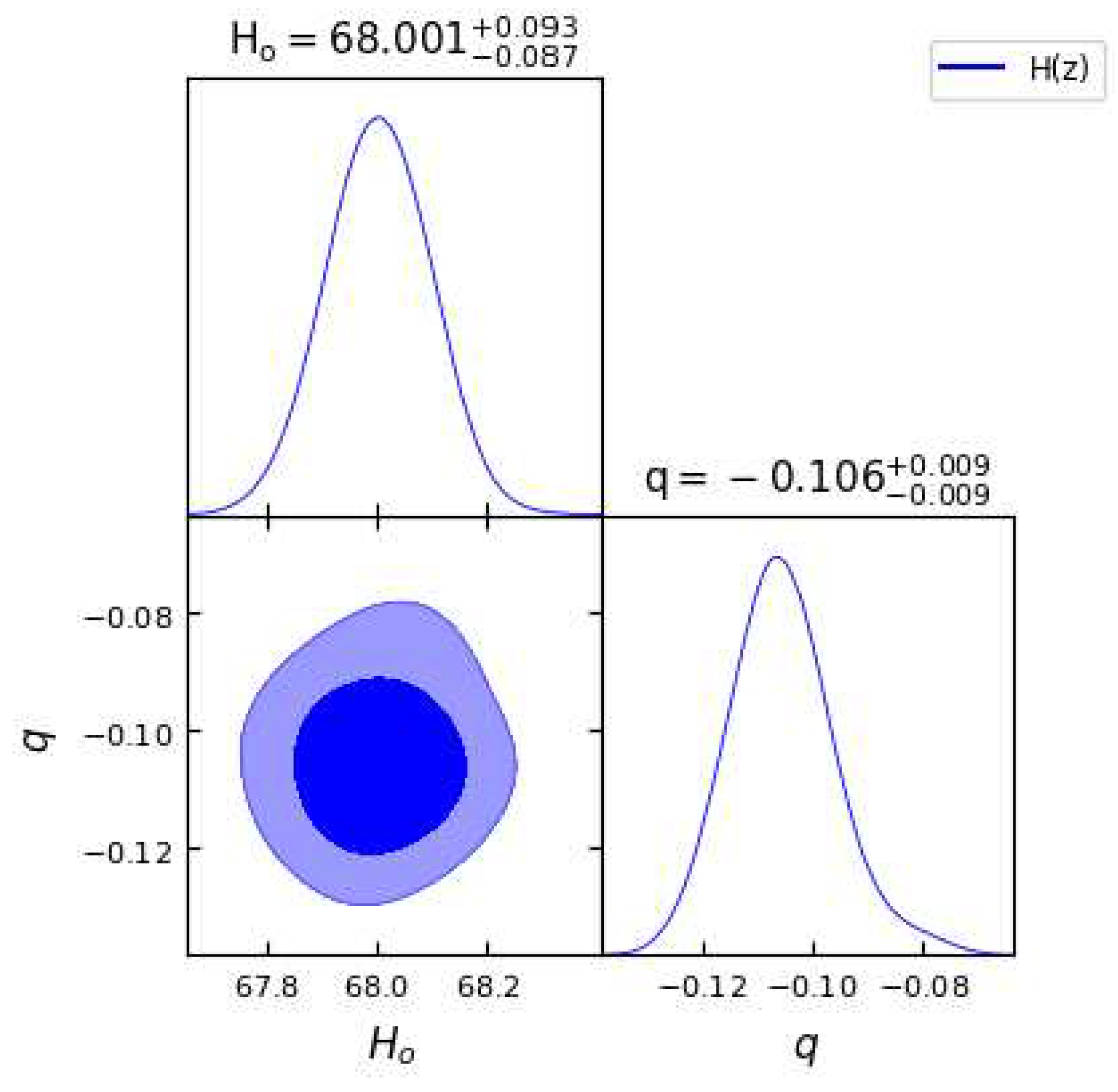
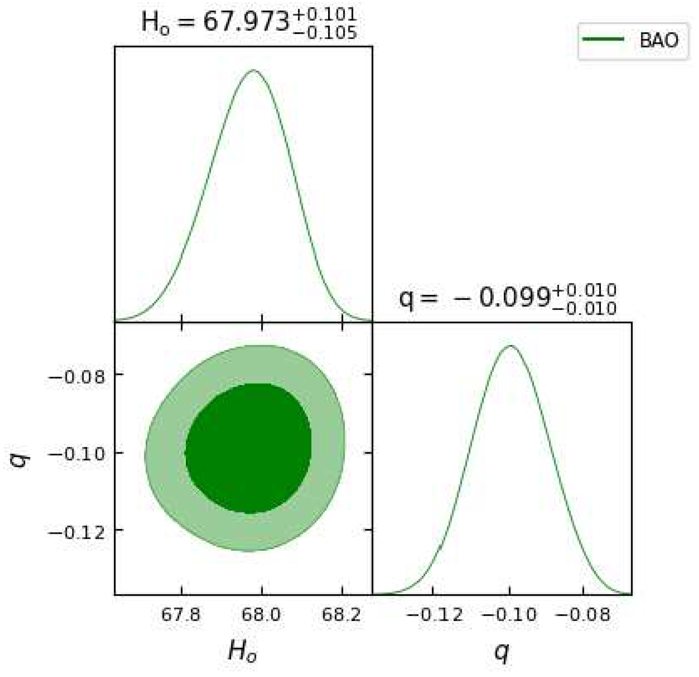
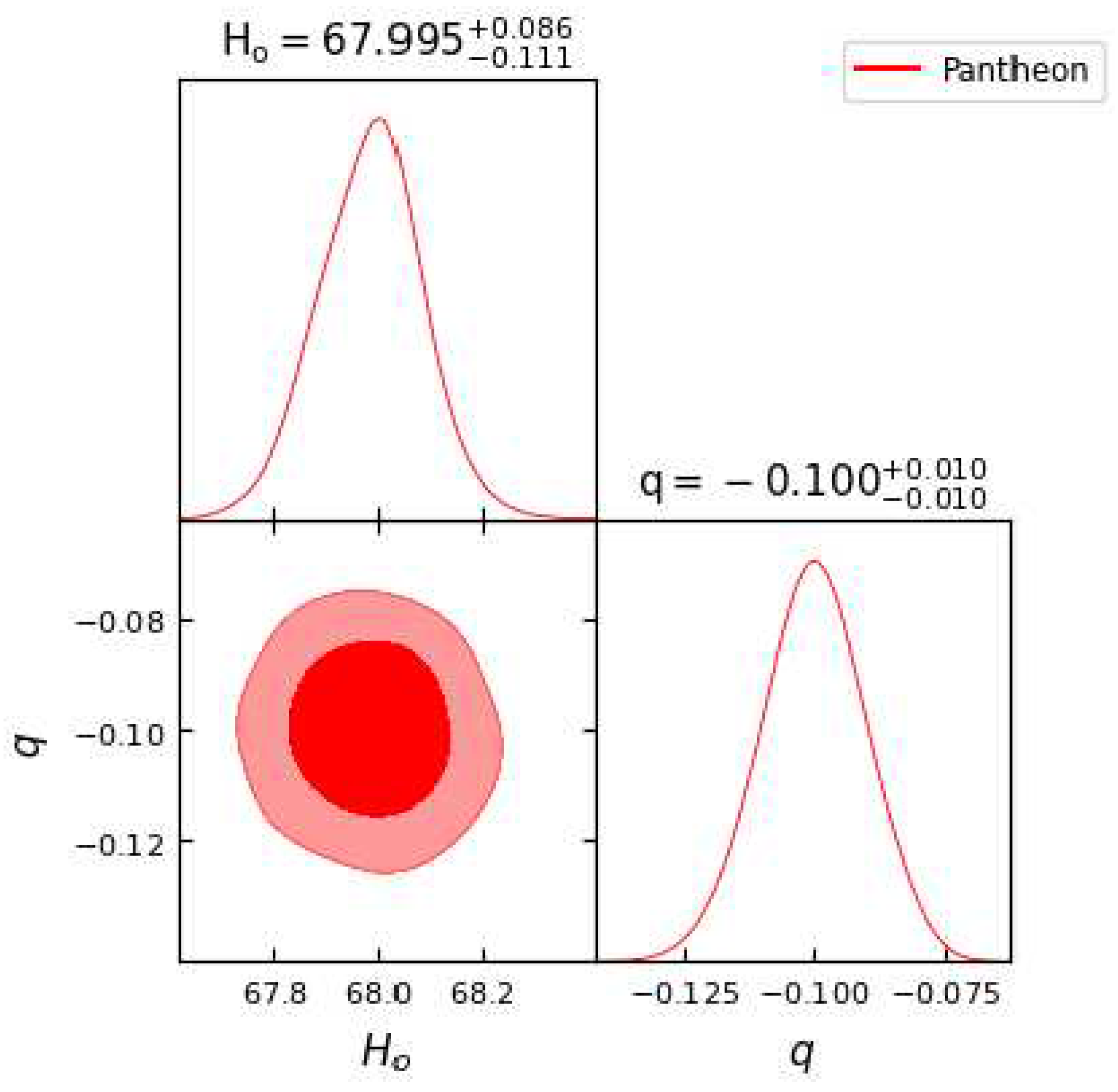
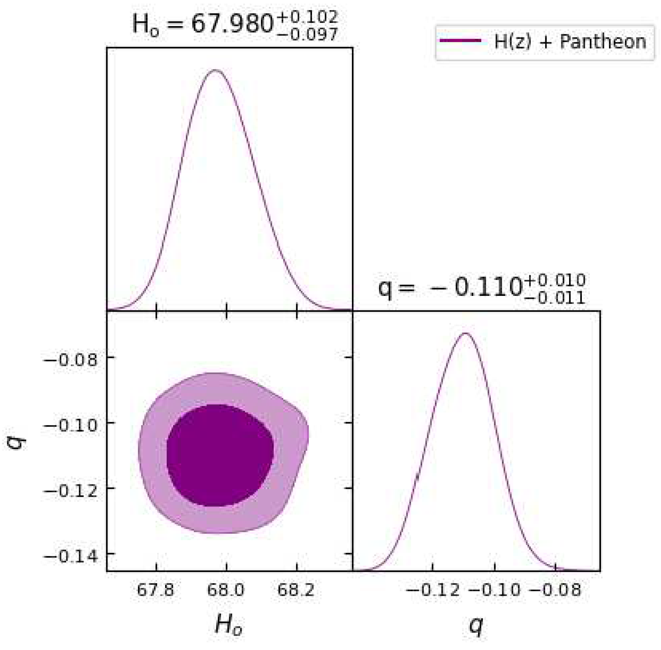
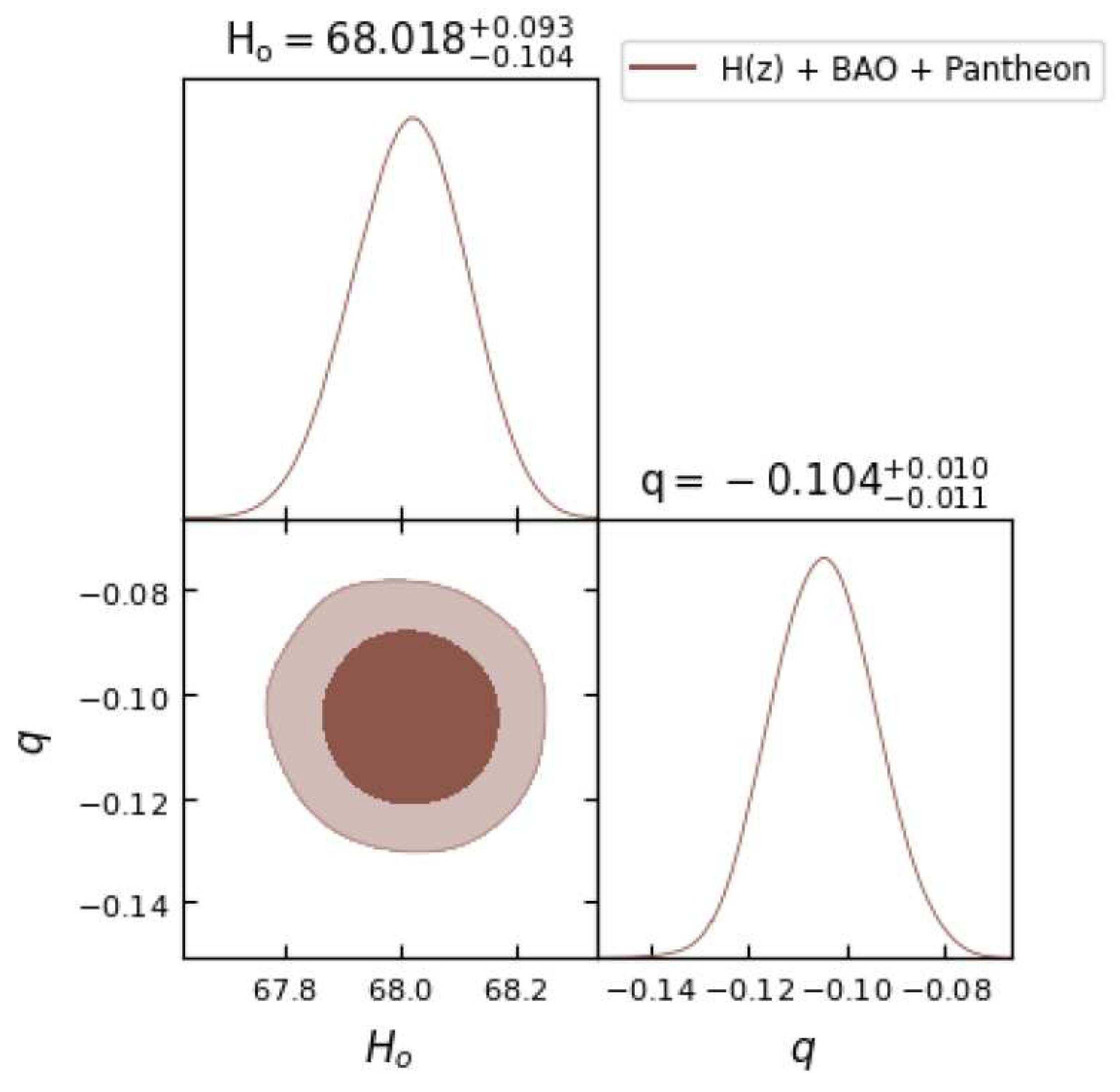
The two-dimensional contour plots for
and
q parameter using the data sets OHD, BAO, Pantheon and their combinations OHD + Pantheon and OHD + BAO + Pantheon are shown in the
Figure 1,
Figure 2,
Figure 3,
Figure 4 and
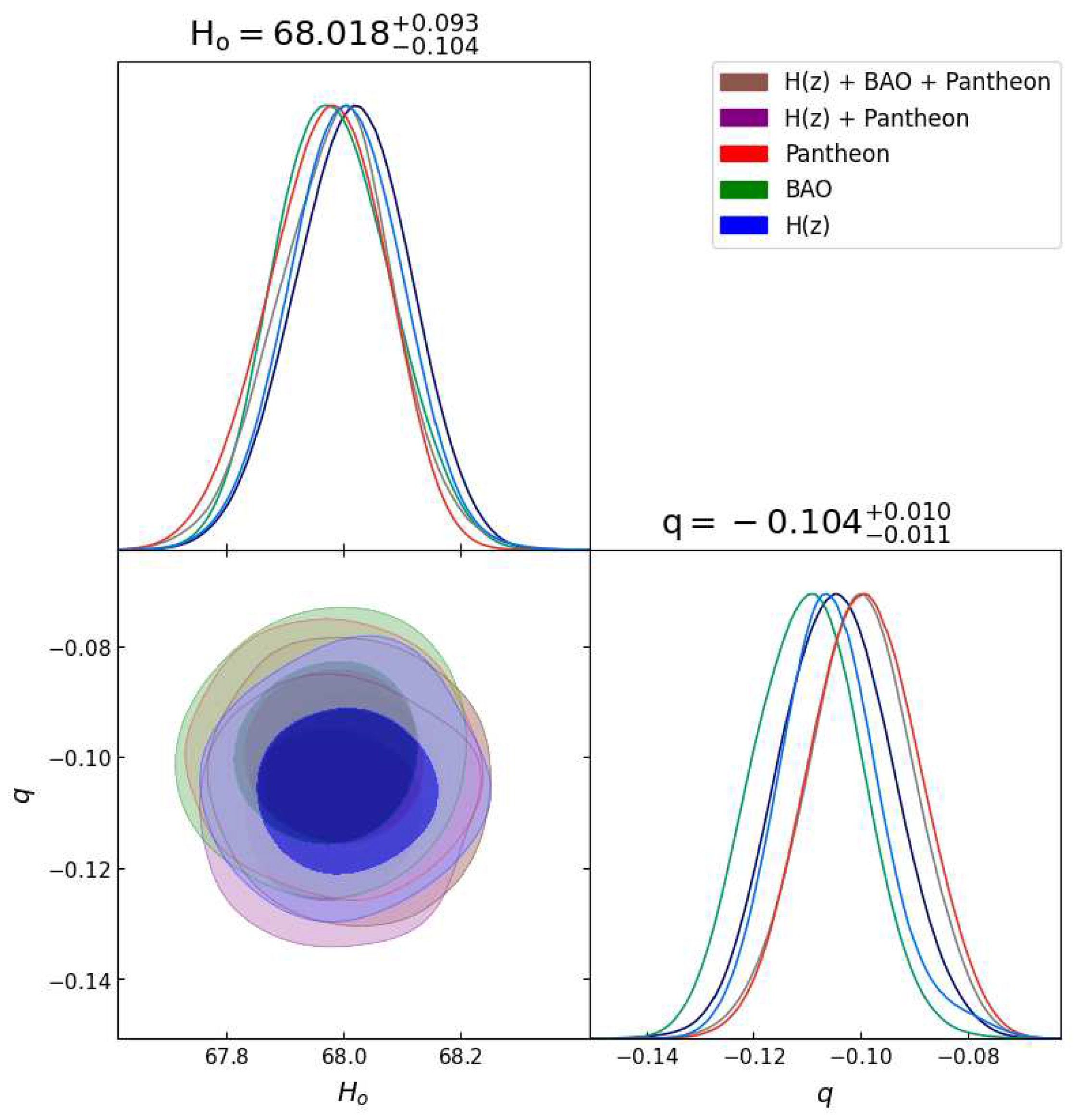
Figure 5 respectively. Their combined nature can be seen in
Figure 6. The obtained values of
and
q parameters by implementing the data sets are presented in
Table 1. We observe that the obtained values of parameter
q are negative, indicating
, which clearly gives the indication of an accelerating universe, as discussed in the theory section.
Figure 1.
In this figure we have exhibited one-dimensional marginalized distribution and two-dimensional contours by using the dataset.
Figure 1.
In this figure we have exhibited one-dimensional marginalized distribution and two-dimensional contours by using the dataset.
Figure 2.
In this figure we have exhibited one-dimensional marginalized distribution and two-dimensional contours by using the BAO dataset.
Figure 2.
In this figure we have exhibited one-dimensional marginalized distribution and two-dimensional contours by using the BAO dataset.
Figure 3.
In this figure we have exhibited one-dimensional marginalized distribution and two-dimensional contours by using the Pantheon dataset.
Figure 3.
In this figure we have exhibited one-dimensional marginalized distribution and two-dimensional contours by using the Pantheon dataset.
Figure 4.
In this figure we have exhibited one-dimensional marginalized distribution and two-dimensional contours by using the combination of and Pantheon dataset.
Figure 4.
In this figure we have exhibited one-dimensional marginalized distribution and two-dimensional contours by using the combination of and Pantheon dataset.
Figure 5.
In this figure we have exhibited one-dimensional marginalized distribution and two-dimensional contours by using the combination of , BAO and Pantheon dataset.
Figure 5.
In this figure we have exhibited one-dimensional marginalized distribution and two-dimensional contours by using the combination of , BAO and Pantheon dataset.
Figure 6.
In this figure we have exhibited one-dimensional marginalized distribution and two-dimensional contours by using the combined variability across all dataset combinations.
Figure 6.
In this figure we have exhibited one-dimensional marginalized distribution and two-dimensional contours by using the combined variability across all dataset combinations.
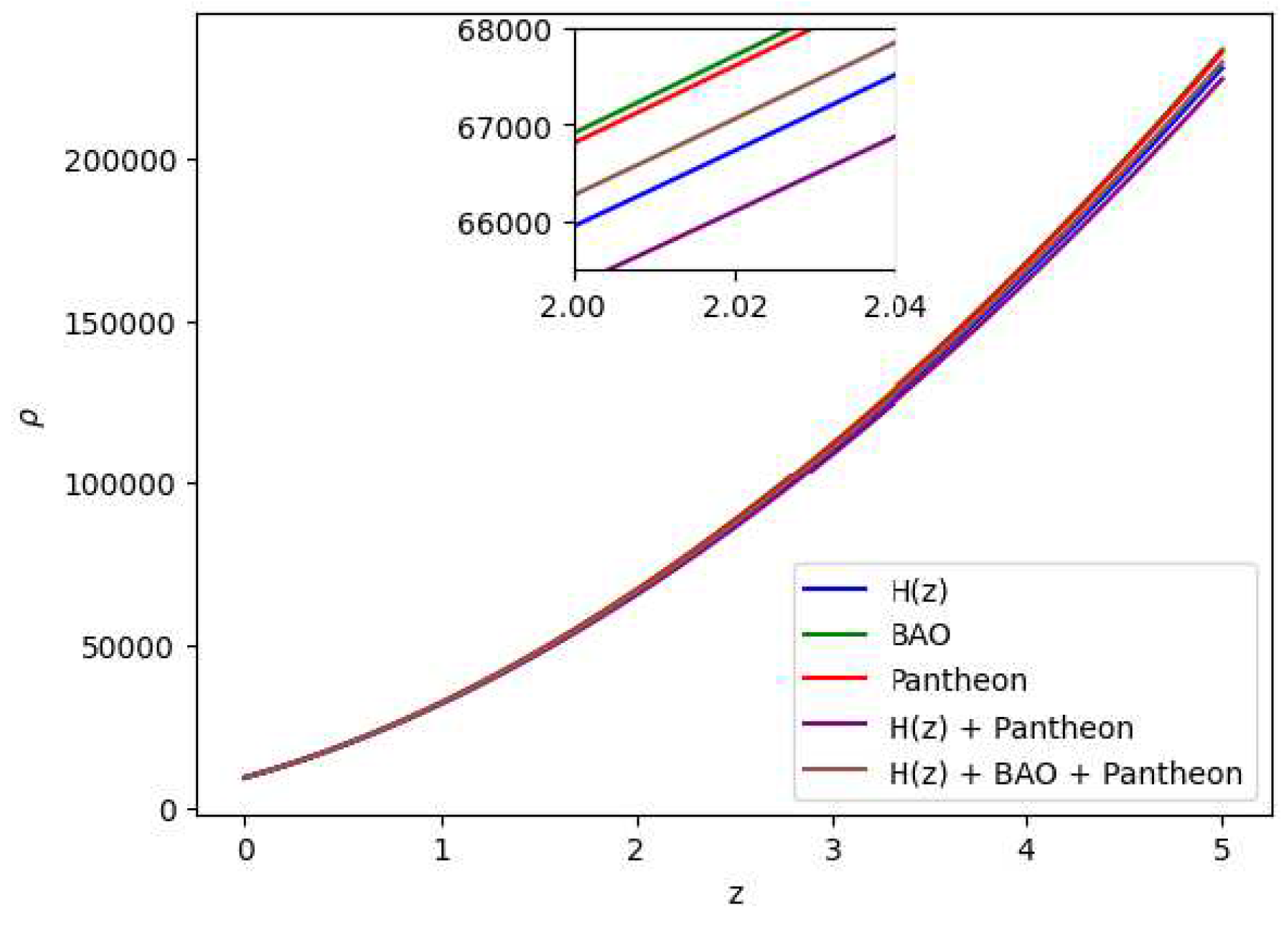
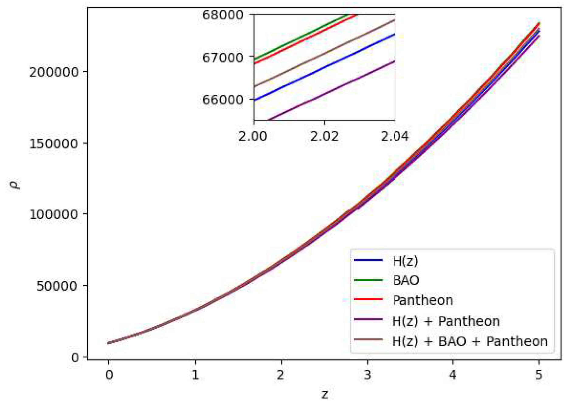
Figure 7.
In this figure we have exhibited the dynamic variation of the energy density () over the redshift (z) under various parameter conditions derived from distinct combinations of the , BAO and Pantheon datasets.
Figure 7.
In this figure we have exhibited the dynamic variation of the energy density () over the redshift (z) under various parameter conditions derived from distinct combinations of the , BAO and Pantheon datasets.
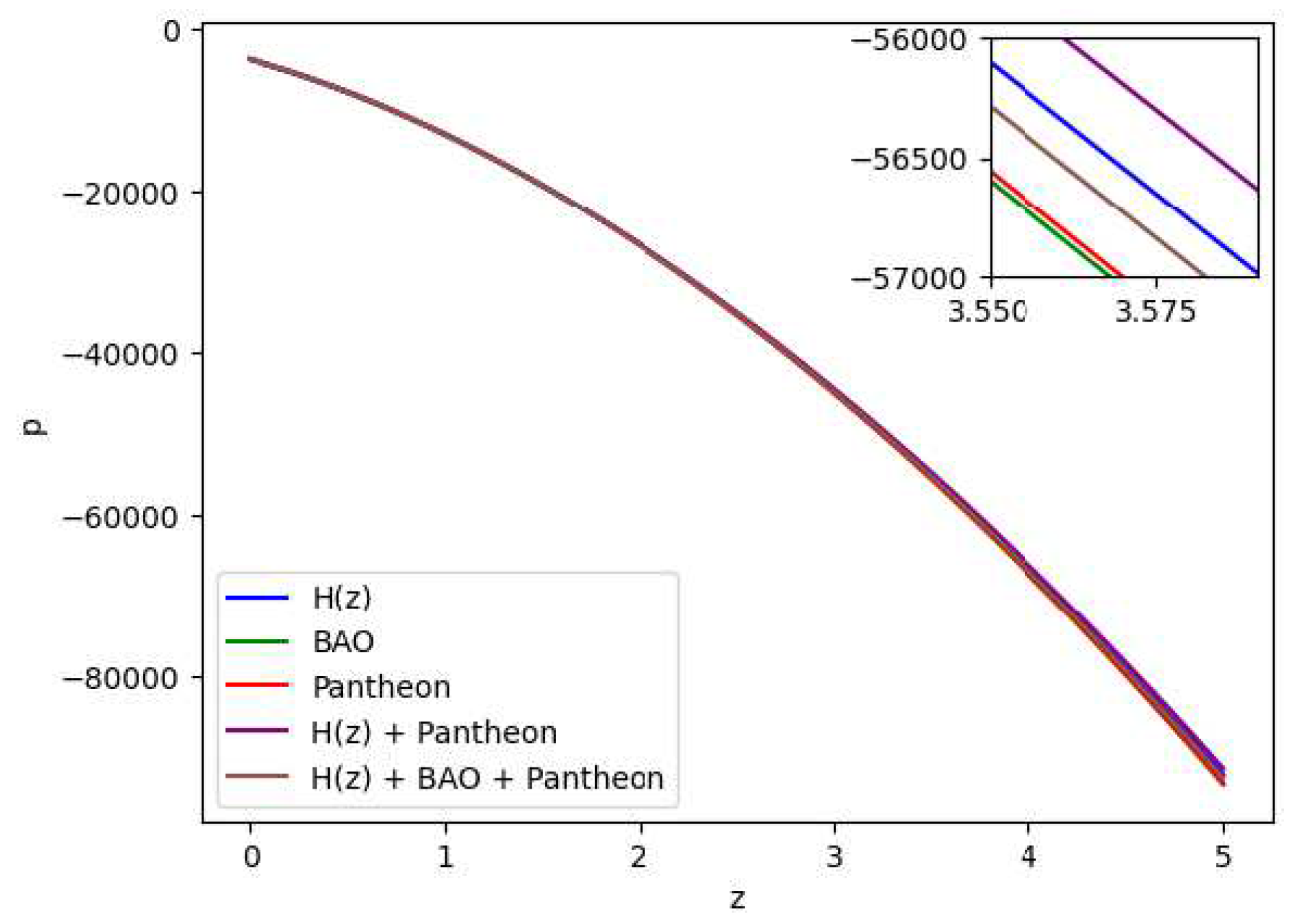
Figure 8.
In this figure we have exhibited the dynamic variation of the pressure (p) over the redshift (z) under various parameter conditions derived from distinct combinations of the , BAO and Pantheon datasets.
Figure 8.
In this figure we have exhibited the dynamic variation of the pressure (p) over the redshift (z) under various parameter conditions derived from distinct combinations of the , BAO and Pantheon datasets.
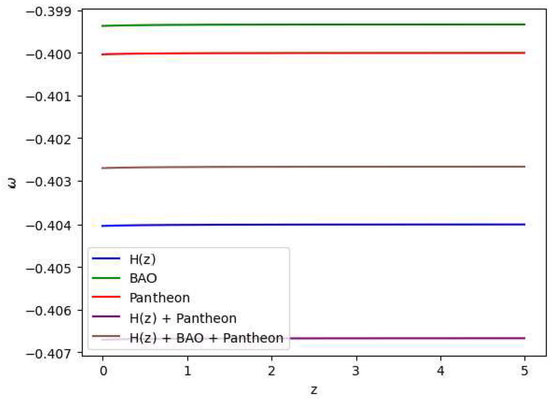
Figure 9.
In this figure we have exhibited variation of the equation of state parameter () vs the redshift (z) which demonstrates that dark energy contributes to the accelerated expansion of the universe, however with a bit variations with the redshift and thus potentially leading to interesting cosmological consequences.
Figure 10.
In this figure we have exhibited the features of the State Finder plots of , and .
Figure 10.
In this figure we have exhibited the features of the State Finder plots of , and .
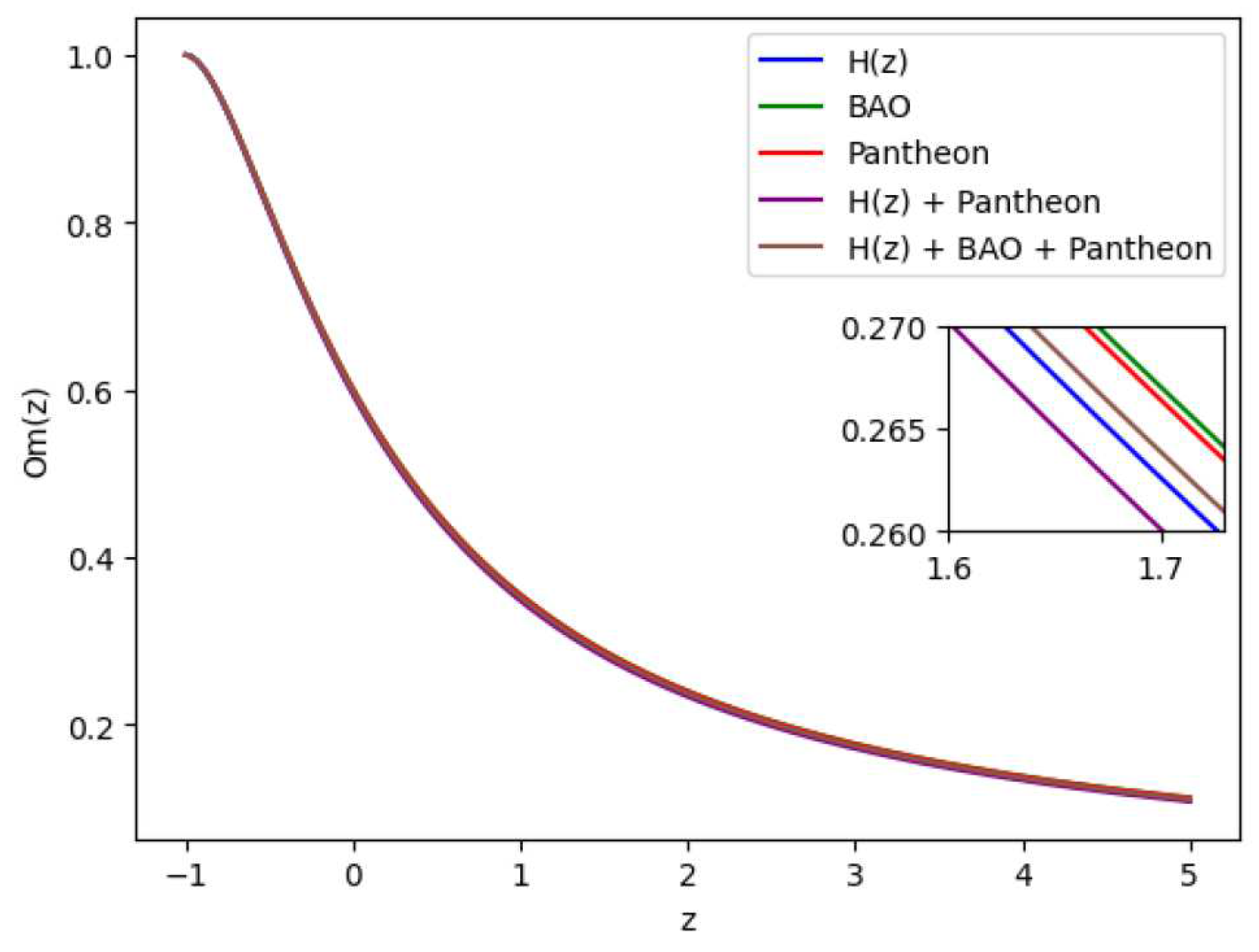
Figure 11.
In this figure we have exhibited variations of with z across for different combined datasets by considering the values obtained from each dataset.
Figure 11.
In this figure we have exhibited variations of with z across for different combined datasets by considering the values obtained from each dataset.
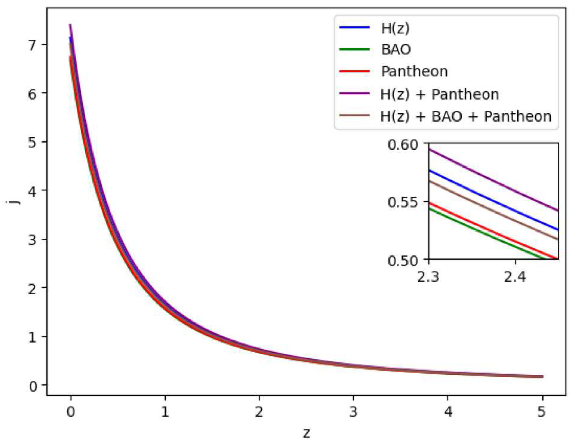
Figure 12.
In this figure we have exhibited the feature of the Jerk parameter j vs z. Here values of j at z = 0 are as follows: for = 7.127 , for BAO = 6.663 , for Pantheon = 6.731 , for + Pantheon = 7.387 and for + BAO + Pantheon = 6.997
Figure 12.
In this figure we have exhibited the feature of the Jerk parameter j vs z. Here values of j at z = 0 are as follows: for = 7.127 , for BAO = 6.663 , for Pantheon = 6.731 , for + Pantheon = 7.387 and for + BAO + Pantheon = 6.997
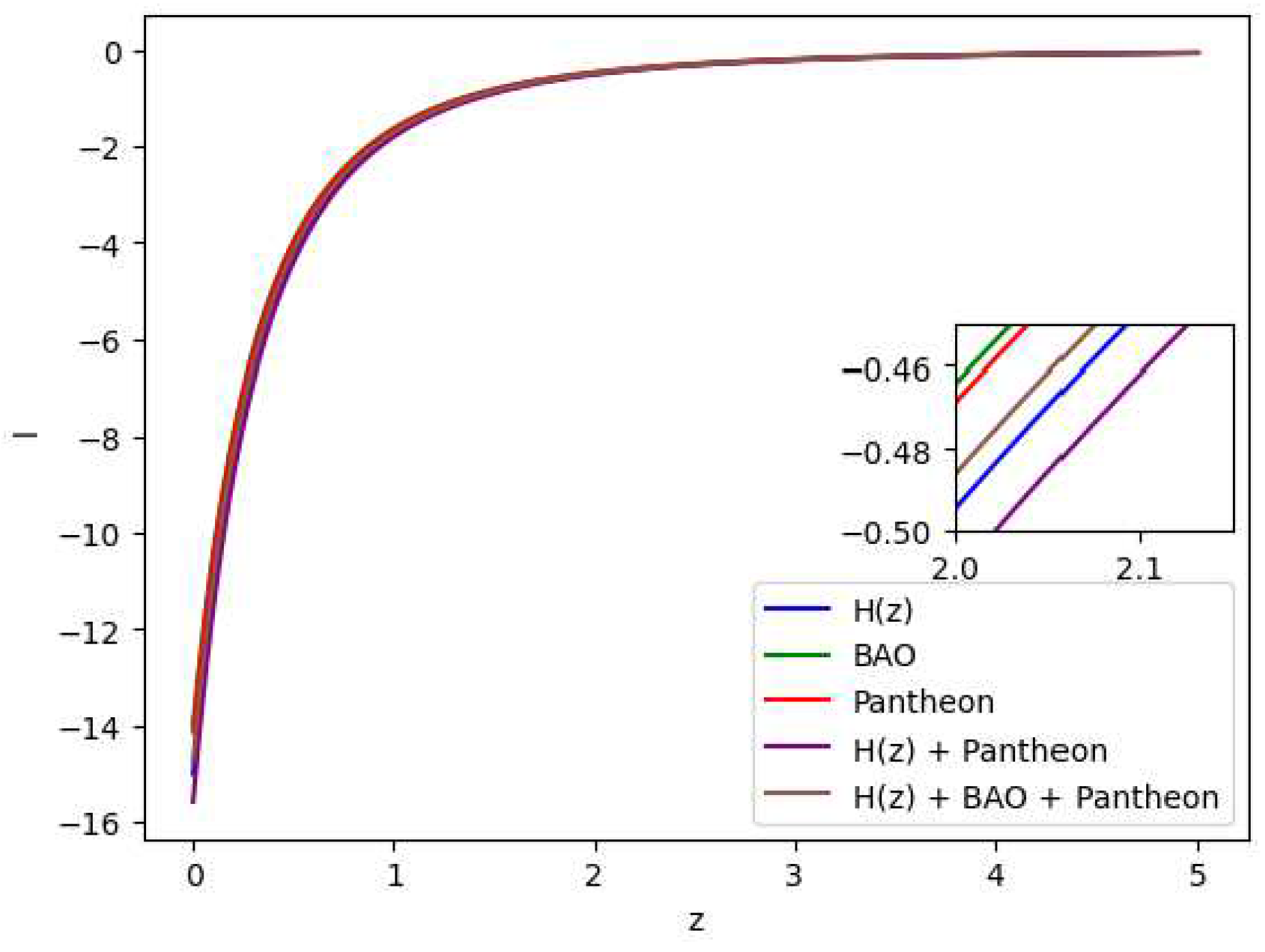
Figure 13.
In this figure we have exhibited the feature of the Lerk parameter l vs z.
Figure 13.
In this figure we have exhibited the feature of the Lerk parameter l vs z.
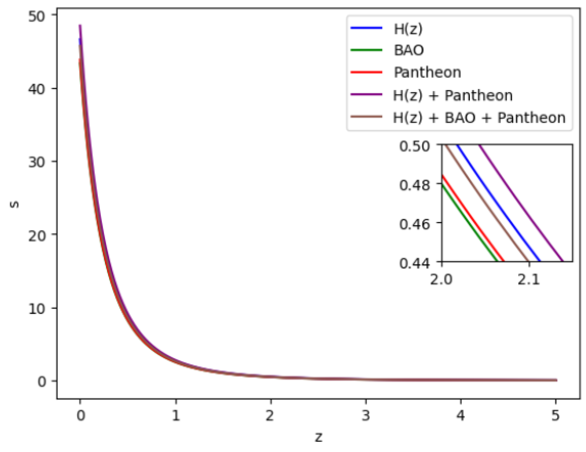
Figure 14.
In this figure we have exhibited the feature of the Snap parameter s vs z.
Figure 14.
In this figure we have exhibited the feature of the Snap parameter s vs z.
4.2. Energy Conditions
Energy conditions (ECs) or similarly construct cosmic principles that explain the distribution of matter and energy across the universe. They are based on Einstein’s gravitational equations and replicate the rules of the cosmos. These circumstances indicate the distribution of matter and energy in space. Hence the energy conditions can be expressed as follows:
- (i)
Weak Energy Condition (WEC): ,
- (ii)
Null Energy Condition (NEC): ,
- (iii)
Strong Energy Condition (SEC): ,
- (iv)
Dominant Energy Condition (DEC): .
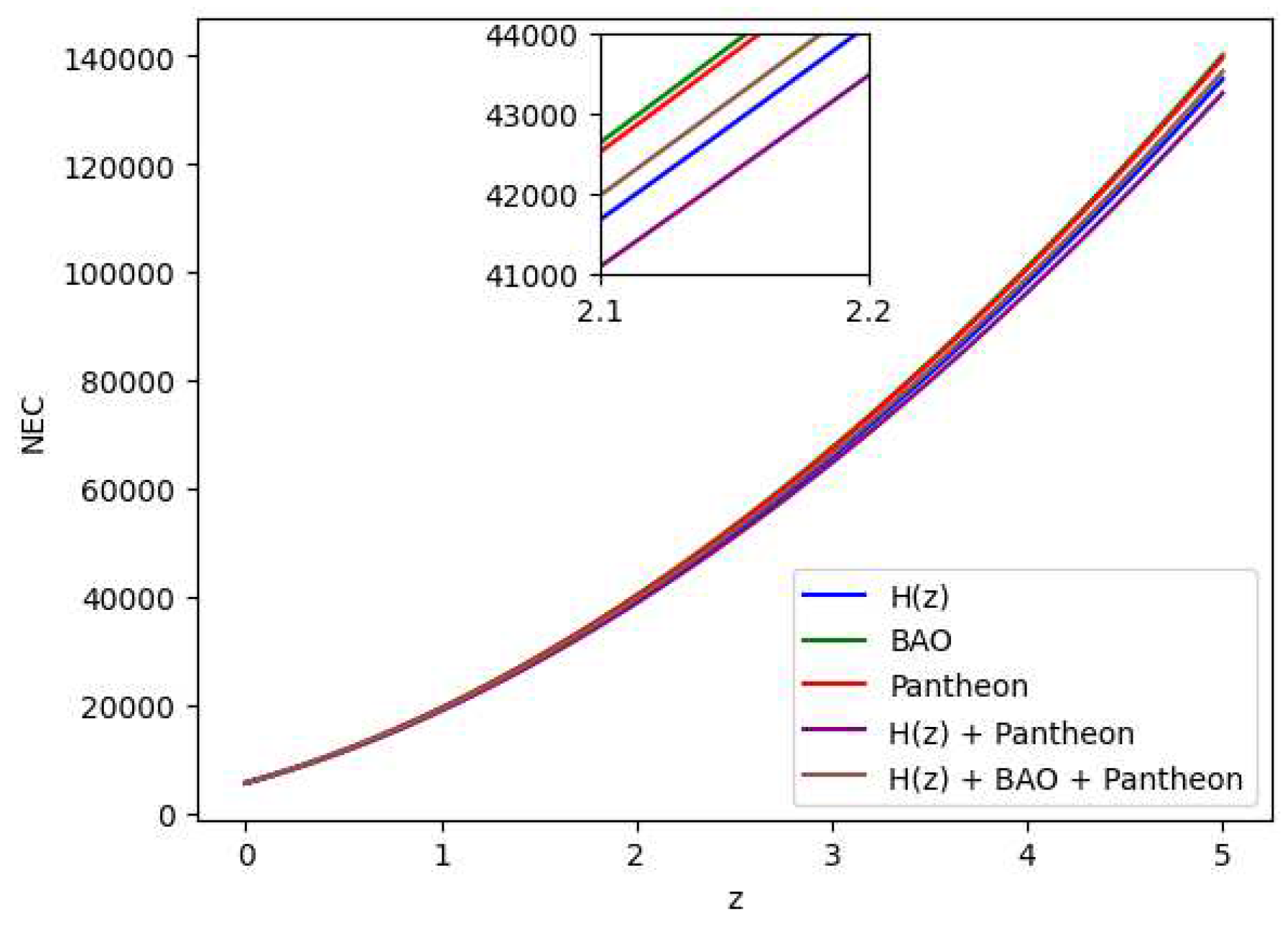
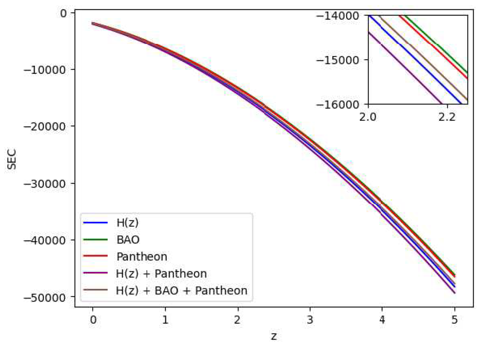
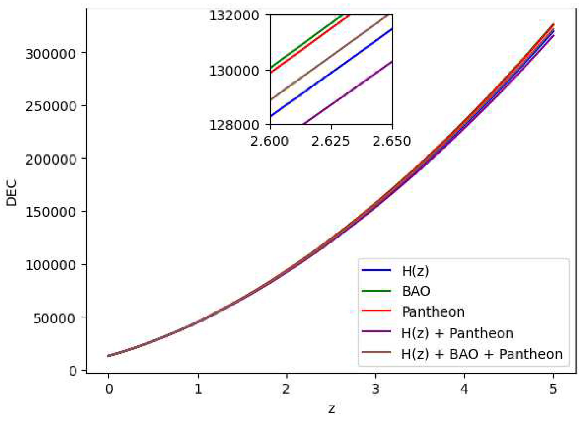
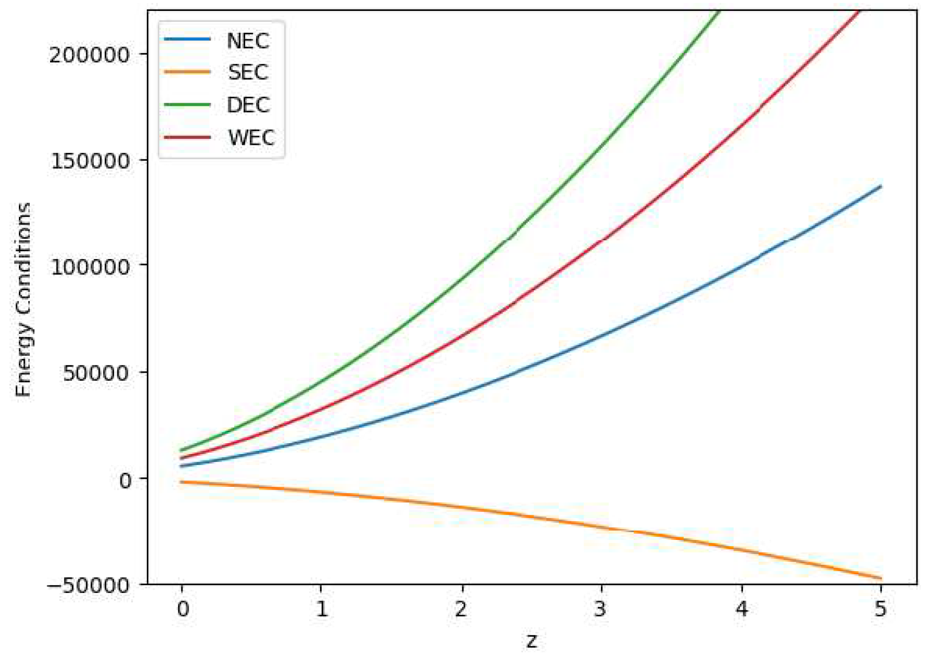
All the energy conditions seperately as well as jointly are shown in
Figure 15,
Figure 16,
Figure 17,
Figure 18 and
Figure 19 by using the Bayesian Analysis of the parameters. Except for Strong Energy Condition (SEC), our results show that Null Energy Condition (NEC), Weak Energy Condition (WEC), and Dominant Energy Condition (DEC) are all satisfied. The SEC violation is justified by the universe’s fast growth. Therefore, the
theory of gravity has potential to explain the current scenario of the late-time acceleration without any need for the cosmological constant as well dark energy in the universe’s energy content. It is to note that the distribution of the energy density
with respect to time
t is shown in
Figure 7, whereas the distribution of the pressure is shown in
Figure 8.
4.3. State Finder Diagnotics
Basically, state finder diagnostics help us to obtain hidden features of the status of dark energy and thus mysteries attached to the history of the universe. As we employ a cosmic compass, these diagnostics lead us through the complexities of cosmic evolution. The r and s parameters are used in state finder diagnostics. Using these characteristics, we can gain a better understanding of the evolution of the universe. Consider them cosmic metres that offer data on the expansion of the universe and its constituent components. These are basically dimensionless parameters which encapsulate the essence of the cosmic development and thus serve as a filter to aid in our understanding of the underlying dynamics of the universe.
Now, the general mathematical expression for the required parameter, expressed in terms of
H, is as follows:
whereas the equations for
r and
s in our model, when expressed in terms of
q, become
The scale factor trajectories in the resulting model may be shown in
Figure 10 to follow a specific set of paths. Our strategy is consistent with the results for the cosmic diagnostic pair from power law cosmology.
4.4. Om(z) parameter
When assessing various dark energy hypotheses in academic works, researchers commonly use the state finder parameters
and the Om diagnosis. The important
parameter is formed when the Hubble parameter
H and the cosmic redshift
z combine which can be defined as
where
corresponds to the current value of the Hubble parameter. According to Shahalam et al. [
69], the negative, zero, and positive values of
indicate the quintessence (
),
CDM, and phantom (
) dark energy (DE) hypotheses, respectively.
The
parameter can be provided for our model as follows:
4.5. Cosmographic Parameters
Many cosmological parameters, given as higher-order derivatives of the scalar component, are examined to comprehend the universe’s expansion history better. As a result, these characteristics are extremely useful for investigating the dynamics of the cosmos. For example, the Hubble parameter
H depicts the universe’s expansion rate, the deceleration parameter
q depicts the universe’s phase transition whereas the jerk parameter
j, snap parameter
s and lerk parameter
l are required to study dark energy theories and their dynamics. These are as follows:
5. Discussion and conclusion
The motivation behind the research paper was to examine the Ricci scalar R and the Gauss-Bonnet invariant G to characterize a cosmological model in flat space-time via gravity. Here we wanted to investigate the observational limitations under a power law cosmology that relies on two parameters - (the Hubble constant) and q (the deceleration parameter) utilizing the 57-point data, 8-point BAO data, 1048-point Pantheon data, joint data of + Pantheon and joint data of + BAO + Pantheon. The outcomes for and q are realistic within observational ranges. As can be noted that our estimate of is remarkably consistent with various recent Planck Collaboration studies under the CDM model.
We have shown via several graphical demonstrations (Figsures 1–19 and Table I) that the obtained values for
and
q satisfactorily correspond to the results observed by the Plank collaboration group. Along with this graphical presentation we have also analyzed the model by studying the energy conditions, the jerk parameter, the lerk parameter and the Om diagnostics as well as the state finder diagnostic tools. According to our study, the power law cosmology within the context of
gravity provides the most comprehensive explanation for the important aspects of cosmic evolution. Furthermore, at the final stage of this paper, we have seen the work of Singh et al. [
70] that prescribes for a cosmological model with power law under the framework of modified theory with higher order curvature term. They [
70] have obtained
,
;
,
and
,
by using
data, Pantheon compilation of SN Ia data and joint data of H(z) + Pantheon respectively. In this paper, the constrained values from the proposed model are as follows:
km s
Mpc
,
;
km s
Mpc
,
;
km s
Mpc
,
;
km s
Mpc
,
;
km s
Mpc
,
by using
data, 8-point BAO data, 1048-point Pantheon data, joint data of
+ Pantheon and joint data of
+ BAO + Pantheon respectively. As a suitable methodology the welknown and effective Markov Chain Monte Carlo (MCMC) has been uniquely employed in the present investigatin.
At this point it is worthwhile to mention that the proposed model has been minimized
tensions and it is calibrated only
,
,
,
and
for
data, 8-point BAO data, 1048-point Pantheon data, joint data of
+ Pantheon and joint data of
+ BAO + Pantheon respectively when we analyzed the estimated values of
in this paper with the value of
obtained by Plank Collaboration [
48]. Moreover, because of the constant value of deceleration parameter
q in power-law cosmology, it could not able to describe the red-shift transition and the proposed model fails to explain the early deceleration phase of the universe. However, one can describes the early deceleration phase of the Universe by choosing appropriate value of
in
. But at the same time one can note that the model fails to explain the late-time acceleration of the Universe.
Finally, even though we have obtained so many useful features, the power-law cosmology seems not a completely packagable technique to study to entire dynamics and eventual fate of the Universe. In this connection, however there may have some scopes to explore thermodynamical aspects, especially entropy, of the late-time acceleration of the Universe and following the works in the Refs. [
70,
71,
72] may be tackled in future projects.
Author Contributions
Conceptualization and writing—original draft preparation, L.K.S.; writing—original draft preparation, S.P. & K.C.K.M.; writing—review and editing, M.K., S.R. & A.K.Y. All authors have read and agreed to the published version of the manuscript.
Funding
The research by M.K. was carried out in Southern Federal University with financial support of the Ministry of Science and Higher Education of the Russian Federation (State contract GZ0110/23-10-IF).
Data Availability Statement
In the present study, we have used available observational data only where no data has been produced in any new form.
Acknowledgments
SR gratefully acknowledges support from the Inter-University Centre for Astronomy and Astrophysics (IUCAA), Pune, India under its Visiting Research Associateship Programme as well as the facilities under ICARD, Pune at CCASS, GLA University, Mathura, India. LKS is also thankful to IUCAA for approving a short visit there when the idea of the present work has been conceived.
Conflicts of Interest
The authors declare no conflict of interest.
References
- Nojiri, S.; Odintsov, S.D.; Tretyakov, P.V. Prog. Theor. Phys. Suppl. 2008 172, 81–89.
- Cognola, G.; Gastaldi, M.; Zerbini, S. Int. J. Theor. Phys. 2008 47, 898–910.
- Bamba, K. Cosmological Issues in F(T) Gravity Theory, arXiv:1504.04457 [gr-qc].
- Odintsov, S.D.; Oikonomou, V.K.; Banerjee, S. Nucl. Phys. B 2019 938, 935–956.
- Yadav, A.K.; Rahaman, F.; Ray, S. Int. J. Theor. Phys. 2011 50, 871–881.
- Yadav, A.K. Astrophys. Space Sci. 2011 335, 565–575.
- Alvarenga, F.G.; de la Cruz-Dombriz, A.; Houndjo, M.J.S.; Rodrigues, M.E.; Sáez-Gómez, D. Phys. Rev. D 2013 87, 103526.
- Das, A.; Rahaman, F.; Guha, B.K.; Ray, S. Eur. Phys. J. C 2016 76, 654.
- Alves, M.E.S.; Moraes, P.H.R.S.; de Araujo, J.C.N.; Malheiro, M. Phys. Rev. D 2016 94, 024032.
- Yadav, A.K. Astrophys. Space Sci. 2016 361, 276.
- Yousaf, Z.; Bamba, K.; Bhatti, M.Z.U.H. Phys. Rev. D 2016 93, 124048.
- Das, A.; Ghosh, S.; Guha, B.K.; Das, S.; Rahaman, F.; Ray, S. Phys. Rev. D 2017 95, 124011.
- Deb, D.; Rahaman, F.; Ray, S.; Guha, B.K. Phys. Rev. D 2018 97, 084026.
- Deb, D.; Ketov, S.V.; Maurya, S.K.; Khlopov, M.; Moraes, P.H.R.S.; Ray, S. Mon. Not. R. Astron. Soc. 2018 485, 5652.
- Sharma, L.K.; Yadav, A.K.; Sahoo, P.K.; Singh, B.K. Res. Phys. 2018 10, 738–742.
- Nagpal, R.; Pacif, S.K.J.; Singh, J.K.; Bamba, K.; Beesham, A. Eur. Phys. J. C 2018 78, 946.
- Sharma, L.K.; Yadav, A.K.; Singh, B.K. New Astron. 2020 79, 101396.
- Sharma, L.K.; Singh, B.K.; Yadav, A.K. Int. J. Geom. Meth. Mod. Phys. 2020 17, 2050111.
- Deb, D.; Ketov, S.V.; Khlopov, M.; Ray, S. J. Cosmol. Astropart. Phys. 2019 10, 070.
- Deb, D.; Rahaman, F.; Ray, S.; Guha, B.K. J. Cosmol. Astropart. Phys. 2019 03, 044.
- Biswas, S.; Ghosh, S.; Guha, B.K.; Rahaman, F.; Ray, S. Ann. Phys. 2019 401, 1–20.
- Biswas, S.; Shee, D.; Ray, S.; Guha, B.K. Eur. Phys. J. C 2020 80, 175.
- Yadav, A.K.; Sharma, L.K.; Singh, B.K.; Sahoo, P.K. New Astron. 2020 78, 101382.
- Biswas, S.; Deb, D.; Ray, S.; Guha, B.K. Ann. Phys. 2021 428, 168429.
- Tripathy, S.K.; Mishra, B.; Khlopov, M.; Ray, S. Int. J. Mod. Phys. D 2021 30, 214000.
- Maurya, S.K.; Tello-Ortiz, F.; Ray, S. Phys. Dark Univ. 2021 31, 100753.
- Singh, A. Eur. Phys. J. C 2023 83, 696.
- Bamba, K.; Capozziello, S.; Nojiri, S.; Odintsov, S.D. Astrophys. Space Sci. 2012 342, 155–228.
- Nojiri, S.; Odintsov, S.D.; Gorbunova, O.G. J. Phys. A 2006 39, 6627.
- Nojiri, S.; Odintsov, S.D. Phys. Lett. B 2005 631, 1–6.
- Cognola, G.; Elizalde, E.; Nojiri, S.; Odintsov, S.D.; Zerbini, S. Phys. Rev. D 2006 73, 084007.
- Li, B.; Barrow, J.D.; Mota, D.F. Phys. Rev. D 2007 76, 044027.
- Elizalde, E.; Myrzakulov, R.; Obukhov, V.V.; Saez-Gomez, D. Class. Quant. Grav. 2010 27, 095007.
- Garcia, N.M.; Lobo, F.S.N.; Mimoso, J.P.; Harko, T. J. Phys. Conf. Ser. 2011 314, 012056.
- Izumi, K. Phys. Rev. D 2014 90, 044037.
- Bamba, K.; Makarenko, A.N.; Myagky, A.N.; Odintsov, S.D. Phys. Lett. B 2014 732, 349–355.
- Escofet, A.; Elizalde, E. Mod. Phys. Lett. A 2016 31, 1650108.
- Oikonomou, V.K. Phys. Rev. D 2015 92, 124027.
- Oikonomou, V.K. Astrophys. Space Sci. 2016 361, 211.
- Makarenko, A.N. Int. J. Geom. Meth. Mod. Phys. 2016 13, 1630006.
- Makarenko, A.N.; Myagky, A.N. Int. J. Geom. Meth. Mod. Phys. 2017 14, 1750148.
- Kleidis, K.; Oikonomou, V.K. Int. J. Geom. Meth. Mod. Phys. 2017 15, 1850064.
- Lohiya, D.; Sethi, M. Class. Quant. Grav. 1999 16, 1545.
- Sethi, M.; Batra, A.; Lohiya, D. Phys. Rev. D 1999 60, 108301.
- Batra, A.; Lohiya, D.; Mahajan, S.; Mukherjee, A. Int. J. Mod. Phys. D 2000 9, 757–773.
- Zhu, Z.H.; Hu, M.; Alcaniz, J.S.; Liu, Y.X. Astron. Astrophys. 2008 483, 15–18.
- Riess, A.G. et al., Astrophys. J. Lett. 2022 934, L7.
- Aghanim, N. et al. [Planck Collaboration], Astron. Astrophys. 2020 641, A6.
- Abdalla, E. et al., JHEP 2022 34, 49–211.
- Perivolaropoulos, L.; Skara, F. New Astron. Rev. 2022 95, 101659.
- Kumar, S.; Nunes, R.C. Phys. Rev. D 2016 94, 123511.
- Kumar, S.; Nunes, R.C.; Yadav, S.K. Eur. Phys. J. C 2019 79, 576.
- Kumar, S. Phys. Dark Univ. 2021 33, 100862.
- de Araujo, J.C.N.; De Felice, A.; Kumar, S.; Nunes, R.C. Phys. Rev. D 2021 104, 104057.
- Hu, J.P.; Wang, F.-Y. Universe 2023 9, 94.
- Vagnozzi, S. Universe 2023 9, 393.
- Kroupa, P. et al., The many tensions with dark-matter based models and implications on the nature of the Universe 2023 arXiv:2309.11552.
- Bernui, A.; Valentino, E.Di; Giare, W.; Kumar, S.; Nunes, R.C. Phys. Rev. D 2023 107, 103531.
- Akarsu, O.; Kumar, S.; Özülker, E.; Vazquez, J.A., Phys. Rev. D 2021 104, 123512.
- Akarsu, O.; Kumar, S.; Özülker, E.; Vazquez, J.A.; Yadav, A. Phys. Rev. D 2023 108, 023513.
- Akarsu, O.; Valentino, E.Di.; Kumar, S.; Nunes, R.C.; Vazquez, J.A.; Yadav, A. ΛsCDM model: A promising scenario for alleviation of cosmological tensions 2023 arXiv.2307.10899.
- Kumar, S. Mon. Not. R. Astron. Soc. 2012 422, 2532–2538.
- Bouali, A.; Chaudhary, H.; Harko, T.; Lobo, F.S.N.; Ouali, T.; Pinto, M.A.S. Mon. Not. R. Astron. Soc. 2023 526, 4192–4208.
- Alam, S. et al., Phys. Rev. D 2021 103, 083533.
- Scolnic D.M. et al. [Pan-STARRS1], Astrophys. J. 2018 859, 101.
- S. Jha, S.; R. P. Kirshner, R.P.; P. Challis, P. et al. Astron. J. 2006 131, 527.
- M. Hicken, M.; P. Challis, P.; S. Jha, S. et al. Astrophys. J. 2009 700, 331.
- Contreras, C.; Hamuy, M.; Phillips, M.M.; Folatelli, G. et al. Astron. J. 2010 139, 519.
- Shahalam, M.; Sami, S.; Agarwa, A. Mon. Not. R. Astron. Soc. 2015 448, 2948–2959.
- Singh, J.K.; Shaily, Pradhan, A.; Beesham, A. Power law cosmology in modified theory with higher order curvature term 2023 arXiv: 2304.09917.
- Debnath, U.; Chattopadhyay, S.; Hussain, I.; Jamil, M.; Myrzakulov, R. Eur. Phys. J. C 2012 72, 1875.
- Manna, G.; Majumder, B.; Das, A. Eur. Phys. J. Plus 2020 135, 107.
|
Disclaimer/Publisher’s Note: The statements, opinions and data contained in all publications are solely those of the individual author(s) and contributor(s) and not of MDPI and/or the editor(s). MDPI and/or the editor(s) disclaim responsibility for any injury to people or property resulting from any ideas, methods, instructions or products referred to in the content. |
© 2024 by the authors. Licensee MDPI, Basel, Switzerland. This article is an open access article distributed under the terms and conditions of the Creative Commons Attribution (CC BY) license (http://creativecommons.org/licenses/by/4.0/).
