Preprint
Article

Uncertainty Analysis of Predictive Models for Water Quality Index: Comparative Analysis of XGBoost, Random Forest, SVM, KNN, Gradient Boosting, and Decision Tree Algorithms.

Submitted:

14 February 2024

Posted:

15 February 2024

You are already at the latest version

A peer-reviewed article of this preprint also exists.

Abstract
Groundwater represents a pivotal asset in conserving natural water reservoirs for potable consumption, irrigation, and diverse industrial uses. Nevertheless, human activities intertwined with industry and agriculture contribute significantly to groundwater contamination, highlighting the critical necessity to appraise water quality for safe drinking and effective irrigation. This research primarily focused on employing the Water Quality Index (WQI) to gauge water's appropriateness for these purposes. However, the generation of an accurate WQI can prove time-intensive owing to potential errors in sub-index calculations. In response to this challenge, an artificial intelligence (AI) forecasting model was devised, aiming to streamline the process while mitigating errors. The study collected 422 data samples from Mirpurkash, a city nestled in the province of Sindh, for a comprehensive exploration of the region's WQI attributes. Furthermore, the study probed into unraveling the interdependencies amidst variables in the physiochemical analysis of water. Diverse machine learning classifiers were employed for WQI prediction, with findings revealing that random forest and gradient boosting eclipsed other algorithms, achieving an accuracy rate of 99%. In close pursuit were SVM and XGBoost, registering accuracy scores of approximately 95% and 93%, respectively, while KNN and Decision Trees garnered accuracy rates of 88% and 87%, respectively. In addition to WQI prediction, the study conducted an uncertainty analysis of the models using the R-factor, providing insights into the reliability and consistency of predictions. This dual approach, combining accurate WQI prediction with uncertainty assessment, contributes to a more comprehensive understanding of water quality in Mirpurkash and enhances the reliability of decision-making processes related to groundwater utilization
Keywords: 
Subject: 
Computer Science and Mathematics  -   Artificial Intelligence and Machine Learning

1. Introduction

Water, as an indispensable resource, plays a fundamental role in sustaining life and supporting various human activities. Among its many sources, groundwater stands as a crucial reservoir essential for drinking, agriculture, and industrial processes in Pakistan. However, the escalating impact of human interventions, particularly in industrial and agricultural sectors, poses a substantial threat to the quality of this invaluable resource [1,2,3,4]. The condition of groundwater in Pakistan, including areas like Mirpurkhas in the province of Sindh, has faced mounting challenges due to extensive usage, urbanization, and agricultural runoff, leading to contamination concerns and a decline in overall quality. The region's reliance on groundwater for daily consumption and agricultural needs amplifies the urgency for effective water quality assessment measures [2,5,6,7]. Contamination of groundwater due to these anthropogenic activities has heightened concerns regarding its suitability for consumption and irrigation purposes, necessitating robust methods for accurate evaluation and monitoring [8,9,10,11].
Traditionally, assessing water quality, especially the determination of the Water Quality Index (WQI), relied heavily on manual calculations and established formulas based on a set of parameters [9,12,13,14,15]. These methods often entail time-consuming processes and are prone to human errors, particularly in complex calculations involving multiple interdependent factors [16,17,18]. In recent years, the integration of artificial intelligence and machine learning techniques, implemented using programming languages like Python, alongside specialized libraries such as scikit-learn, XGBoost, and pandas, has emerged as a transformative approach to overcome the limitations of traditional methods. Machine learning models, such as Random Forest, Gradient Boosting, Support Vector Machines (SVM), K-Nearest Neighbors (KNN), and Decision Trees, were developed and trained using these tools. They offer the advantage of learning patterns and relationships from vast datasets, enabling more accurate and efficient prediction of WQI [19,20,21].
This study, conducted in the geographic area of Mirpurkhas in Sindh, collected an extensive dataset of 422 samples to comprehensively understand the region's water quality characteristics. Leveraging Python and various machine learning libraries such as scikit-learn, XGBoost, and pandas, the research employed these tools to preprocess data, build, train, and evaluate machine learning classifiers for predicting WQI [22,23]. The results indicated that Random Forest and Gradient Boosting outperformed other algorithms, achieving an exceptional accuracy rate of 99%. Following closely were SVM and XGBoost, scoring approximately 95% and 93% accuracy, respectively, while KNN and Decision Trees demonstrated accuracy rates of 88% and 87%, respectively. These findings underscore the efficacy of Python-based machine learning techniques implemented with specialized libraries in accurately predicting WQI, showcasing their potential for advancing water quality assessment methods, particularly in groundwater evaluation [24,25,26]. Through an interdisciplinary approach integrating environmental science and machine learning, this research aims to contribute to the advancement of accurate and efficient water quality assessment methods, utilizing the potential of artificial intelligence and predictive modeling implemented through Python-based tools and specialized libraries.
Beyond WQI prediction, this study integrates an uncertainty analysis using the R-factor, providing a nuanced perspective on the reliability and consistency of our predictive models. The combined approach of accurate WQI prediction and uncertainty assessment contributes to a more holistic understanding of water quality dynamics in Mirpurkash. Ultimately, this research aims to inform robust decision-making processes regarding groundwater utilization, considering both the accuracy of predictions and the inherent uncertainties associated with them. The integration of artificial intelligence (AI) forecasting models, specifically machine learning classifiers, such as Random Forest, Gradient Boosting, SVM, XGBoost, KNN, and Decision Trees, has proven to be instrumental in predicting the Water Quality Index (WQI) with remarkable accuracy. However, the accuracy of predictions alone does not provide a complete picture, and understanding the structure of these models is essential for a comprehensive assessment of uncertainty.
The research paper is structured to encompass several key sections. Beginning with an Introduction that highlights the significance of groundwater, particularly in the context of Mirpurkhas in Sindh, it emphasizes the challenges of water quality and the need for advanced assessment methods, summarizing previous studies on groundwater quality, traditional Water Quality Index (WQI) determination methods, their limitations, and existing research on applying machine learning in water quality assessment. The Methodology section outlines the steps undertaken, including data collection of 422 samples, data preprocessing, feature selection, and the utilization of machine learning algorithms such as Random Forest, Gradient Boosting, SVM, XGBoost, KNN, and Decision Trees and evaluation of uncertainty in above machine learning algorithms. The subsequent Results section presents the performance metrics of these models in predicting WQI accuracy rates. Following this, the Discussion interprets the outcomes, compares model performances, addresses limitations, and suggests further research avenues. Finally, a Conclusion summarizes the key findings, reinforces the significance of employing machine learning in water quality assessment, and suggests future implications.

2. Materials and Methods

2.1. Study Area

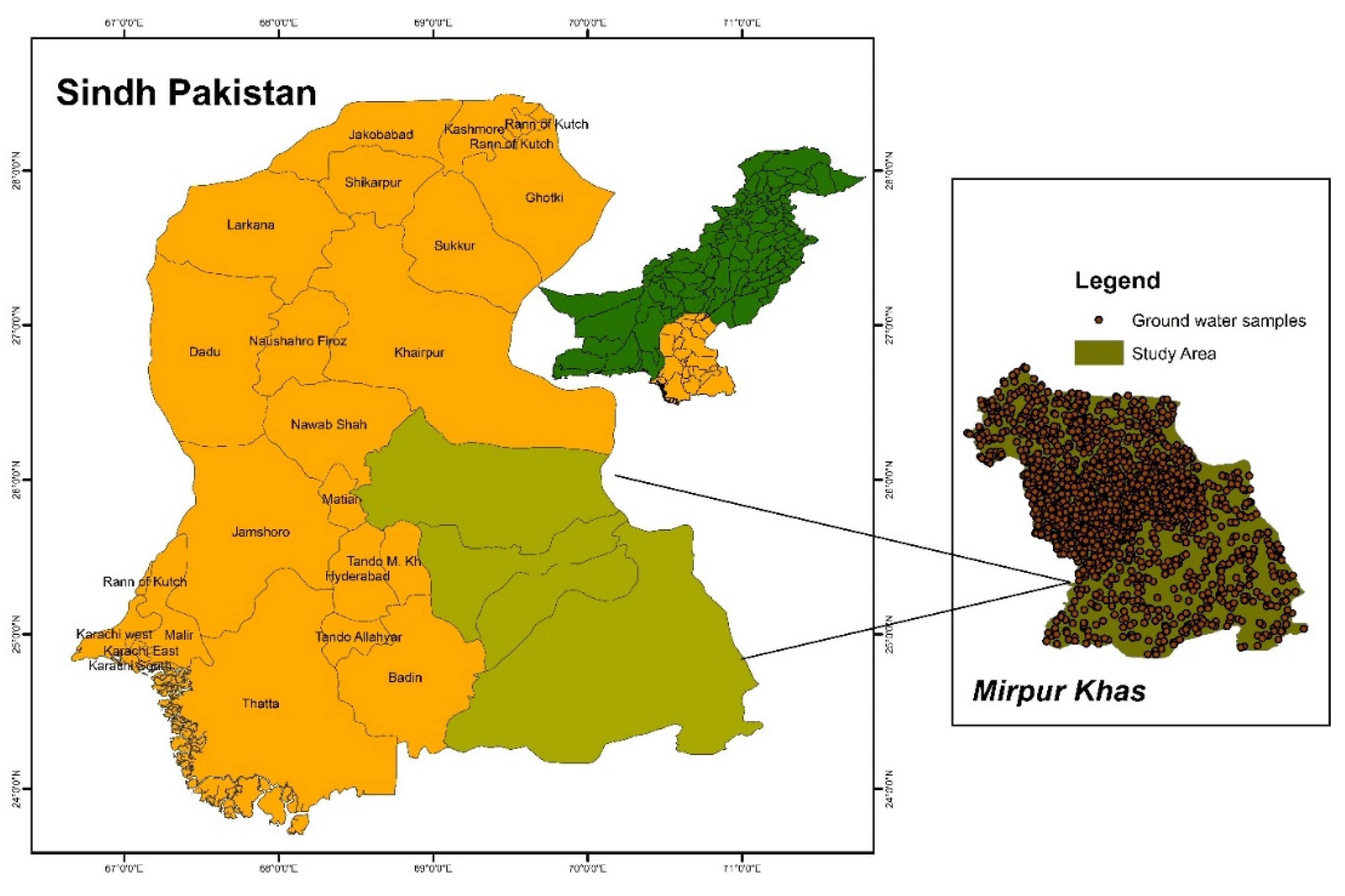
Mirpurkhas, situated in the Sindh province of Pakistan, experiences an arid to semi-arid climate characterized by scorching summers with temperatures often exceeding 40 degrees Celsius (104 degrees Fahrenheit) from April to September. Monsoons, occurring between July and September, bring moderate to heavy rainfall, providing relief from the intense heat. Winters are relatively mild, ranging from around 10 to 20 degrees Celsius (50 to 68 degrees Fahrenheit). Geographically, Mirpurkhas is located near the Indus River in the southern part of Pakistan and is renowned for its agricultural activities [7,27]. Wells play a crucial role in providing groundwater for various purposes, including drinking water supply and agricultural irrigation, supporting the local livelihoods within this semi-arid region.
Mirpurkhas, a town located in the Sindh province of Pakistan, heavily relies on well water for various purposes. The inhabitants of Mirpurkhas primarily utilize well water for drinking, agricultural irrigation, and domestic needs [28,29]. Wells in the region serve as a primary source of groundwater, supplying water to the local community. The quality of well water in Mirpurkhas is crucial for sustaining daily activities and agricultural practices. However, like many areas reliant on groundwater, the water quality in wells can be susceptible to contamination from various sources such as agricultural runoff, industrial activities, and natural factors [30,31,32].
Figure 1. study area and ground water sampling points.
Preprints 98939 g001

2.2. Methodology

The research methodology involved the collection of 422 water samples from multiple sites across Mirpurkhas, Sindh, Pakistan, covering various locations deemed significant for groundwater extraction and consumption. Parameters including pH levels, temperature, dissolved oxygen, turbidity, nitrates, and other physiochemical characteristics were measured using standardized water testing procedures and equipment [33,34,35]. Following data collection, a rigorous preprocessing phase was conducted to ensure data accuracy and suitability for machine learning analysis. This stage encompassed handling missing values through imputation methods, outlier removal, and normalization or scaling to ensure uniformity across parameters. Feature engineering was performed to extract pertinent features and reduce dimensionality for enhanced model performance. Feature selection techniques were employed, including Variance Inflation Factor (VIF) and Information Gain (IG), to identify influential parameters affecting water quality. These methods aimed to reduce redundancy and select the most informative features for modeling [36,37].
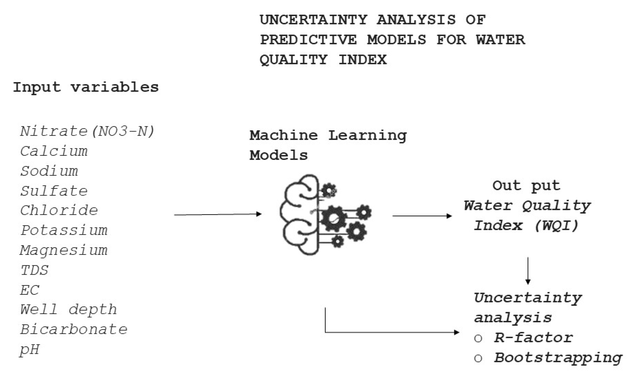
For model development, Python programming language was utilized along with machine learning libraries such as scikit-learn, XGBoost, pandas, and numpy. Supervised learning algorithms, including Random Forest, Gradient Boosting, Support Vector Machines (SVM), XGBoost, K-Nearest Neighbors (KNN), and Decision Trees, were implemented and trained using the preprocessed dataset [38,39]. Hyperparameter tuning through techniques like grid search and cross-validation optimized the models. The performance of the developed models was evaluated using common metrics such as accuracy, confusion matrix , Friedman test and Nemenyi test [40,41]. The uncertainty of models predictions has been evaluated using R-factor and Bootstrapping.
Figure 2. Methodology used for predicting water quality index for given input variables.
Preprints 98939 g002
The data underwent resampling using a 5-fold cross-validation technique to assess model robustness and generalizability. The dataset was divided into 70% training and 30% testing subsets to validate model predictions on unseen data [42]. Results interpretation involved comparing and analyzing the outcomes of various machine learning classifiers to identify the most accurate models for predicting the Water Quality Index (WQI). Models demonstrating the highest accuracy rates were further analyzed to understand the impact of different parameters on WQI prediction and water quality assessment.
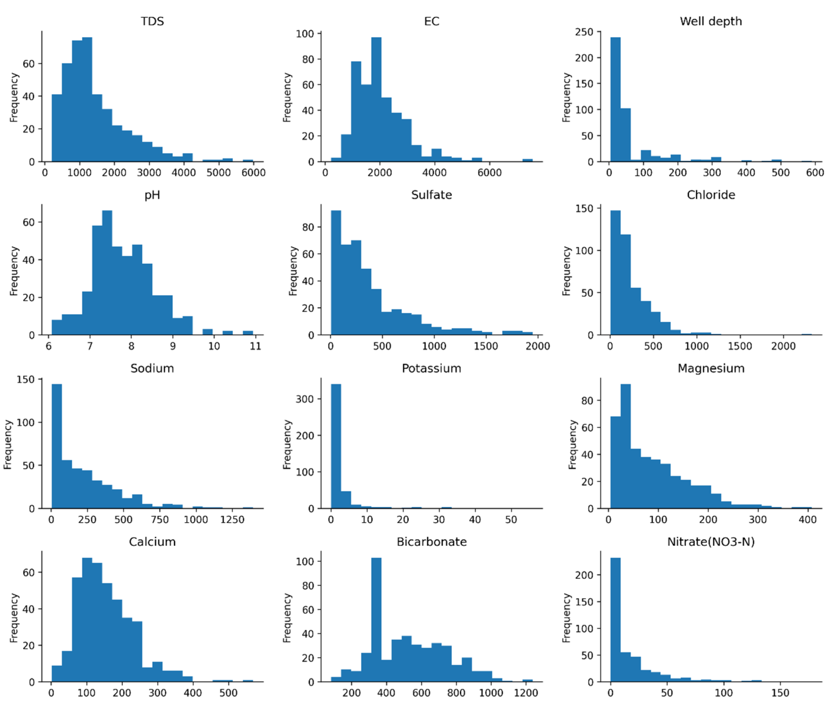
The variables that have been used in our research to determine the water quality index are shown in Figure 3.
The VIF analysis highlights varying degrees of multicollinearity among the features considered for water quality assessment in Mirpurkhas, Sindh, Pakistan. Notably, certain parameters, such as 'TDS', 'Sodium', 'Calcium', and 'Magnesium', exhibited notably high VIF values, indicative of strong multicollinearity among these variables. Conversely, 'Potassium', 'Well Depth', and 'Nitrate (NO3-N)' demonstrated relatively lower VIF values, suggesting lower levels of multicollinearity in comparison [43].
Table 1. Variance Inflation Factor (VIF) values indicating multicollinearity among water quality assessment features in Mirpurkhas, Sindh, Pakistan.
Feature VIF
TDS 4209.78
Sodium 1137.34
Calcium 425.13
Magnesium 380.55
Bicarbonate 58.74
Sulfate 39.68
Chloride 31.69
pH 20.16
EC 10.20
Nitrate (NO3-N) 5.45
Well Depth 1.70
Potassium 1.43
The Variance Inflation Factor (VIF) values, obtained from the assessment of water quality parameters in Mirpurkhas, Sindh, reveal varying degrees of multicollinearity among features considered for predicting the Water Quality Index (WQI). Features such as 'TDS', 'Sodium', 'Calcium', and 'Magnesium' exhibit notably high VIF values, suggesting strong interdependencies among these variables. This significant multicollinearity potentially impacts the accuracy of predictive models developed for water quality assessment [44]. Parameters with lower VIF values, including 'Potassium', 'Well Depth', and 'Nitrate (NO3-N)', indicate weaker correlations, potentially posing less influence on multicollinearity issues within predictive models. Addressing high multicollinearity, particularly among variables with elevated VIF values, becomes crucial in enhancing the reliability and precision of predictive models for more accurate water quality assessment in the Mirpurkhas region.
Table 2. Information Gain (IG) values indicating corresponding information gain of each water quality assessment feature in Mirpurkhas, Sindh, Pakistan.
Feature IG
Nitrate (NO3-N) 0.876
Calcium 0.869
Sodium 0.869
Sulfate 0.869
Chloride 0.869
Potassium 0.869
Magnesium 0.869
TDS 0.816
EC 0.784
Well Depth 0.525
Bicarbonate 0.520
pH 0.509
The Information Gain (IG) analysis highlights the relevance of various features in predicting the Water Quality Index (WQI) in Mirpurkhas, Sindh, Pakistan. Features such as 'Nitrate (NO3-N)', 'Calcium', 'Sodium', 'Sulfate', 'Chloride', 'Potassium', and 'Magnesium' exhibit higher IG values, indicating their considerable relevance in predicting WQI. Conversely, 'pH', 'Bicarbonate', 'Well Depth', 'EC', and 'TDS' present relatively lower IG values, suggesting comparatively lesser impact in predicting the WQI. Understanding the relevance of these features assists in selecting the most influential variables for the development of accurate predictive models for water quality assessment.
However, it's important to note that while IG values help identify influential features, the absolute value of IG alone might not necessarily determine the direct impact or importance of a feature in predicting the WQI [45]. Other factors such as domain knowledge, the nature of the dataset, and the specific context of the water quality assessment should also be considered when selecting influential variables for building accurate predictive models. Therefore, while IG values provide valuable insights, the selection of the most influential variables should involve a comprehensive analysis that integrates multiple factors beyond IG values alone.

Uncertainty Analysis

R-factor 

While various factors contribute to the uncertainty in predicting Water Quality Index (WQI), including modeling, sampling errors, data preparation, and pre-processing, this study specifically addresses the uncertainty linked to individual model structures and input parameter selection. To assess model structure uncertainty, the analysis involves examining a set of three predicted WQI values during the testing phase for each observed WQI. These predictions are generated by the aforementioned predictive models.
The mean and standard deviation are computed for each predicted set, serving as parameters for a designated normal distribution function. Employing the 'Monte Carlo' simulation method, 1000 WQI values are generated for each observed value based on this distribution. While other methods like Latin Hypercube [46] , Lagged Average [47], and Multimodal Nesting [48] are utilized for sample generation, the Monte Carlo technique has demonstrated greater applicability, especially in hydrology and water-related sciences [49]. To quantify the uncertainty associated with WQI prediction, the 95% prediction confidence interval (i.e., the interval between the 97.5% and 2.5% quantiles), known as the prediction uncertainty of 95% (95PPI), is determined using the generated WQI values for each observed WQI. Specifically, the uncertainty is computed using the defined R-factor equation (1).
The formula for the calculation of the R-factor is expressed as:
R f a c t o r = s p s x         ( 1 )
Here, s x   represents the standard deviation of the observed values, and s p   is determined using Equation (2):
s p = i = 1 J ( U L i L L i ) J             ( 2 )
In this equation, J denotes the number of observed data points, while U L i and L L i correspond to the i-th values of the upper quartile (97.5%) and lower quartile (2.5%) of the 95% prediction confidence interval band (95PPI).
Other approaches, such as the Coefficient of Variation (CV), Prediction Interval Coverage Probability (PICP), and Prediction Interval Normalized Root-mean-square Width (PINRW), have been proposed as substitutes for the R-factor method [50]. Nevertheless, these alternative methods solely rely on either observed or predicted data. In contrast, the R-factor method takes into account both observed and predicted data, making it a more comprehensive metric for characterizing prediction uncertainty [51,52]. The inherent uncertainty in predictive models arises from various sources, including the complexity of the underlying data and the dynamic nature of water quality parameters. The structure of machine learning models contributes significantly to this uncertainty, and exploring their characteristics sheds light on the reliability of predictions.

Bootstrapping

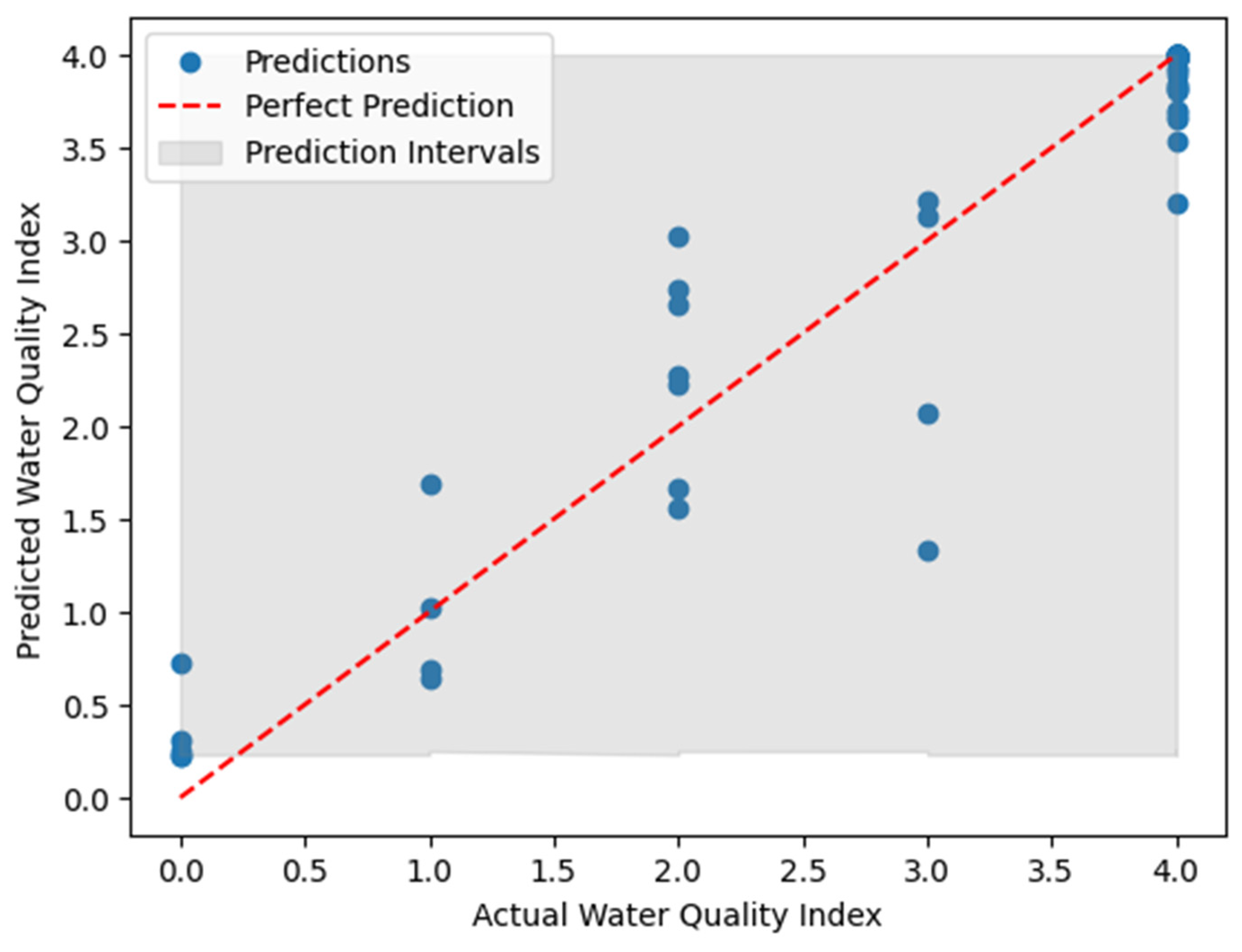
In the uncertainty analysis of predictive models for water quality index, generating prediction intervals is crucial for understanding the range of possible values for each prediction. This step involves using bootstrapping, a resampling technique that provides a measure of the uncertainty associated with the model's predictions. Bootstrapping involves creating multiple bootstrap samples by randomly drawing observations with replacement from the original dataset. For each bootstrap sample, the model is trained, and predictions are made on the test set. This process is repeated numerous times (in our case, 1000 iterations), resulting in a distribution of predicted values for each data point.
Interpretation of Mean Squared Error (MSE) : The Mean Squared Error on the Test Set (0.108) indicates the average squared difference between the actual water quality index values and the predicted values. A lower MSE generally suggests better model performance, demonstrating that the model's predictions are, on average, close to the true values.
However, the MSE alone may not provide a complete picture, as it does not account for the uncertainty in the predictions. This is where prediction intervals come into play. The generated prediction intervals using bootstrapping offer insights into the variability and uncertainty associated with the model's predictions. The lower and upper bounds of the intervals (calculated at the 2.5th and 97.5th percentiles, respectively) represent the plausible range within which the true water quality index values are likely to fall. The scatter plot (Figure 4 )of actual versus predicted values, along with the shaded gray area representing the prediction intervals, provides a clear visualization of the model's performance and the associated uncertainty. The narrower the prediction intervals, the more confident we can be in the model's predictions.
A narrow prediction interval suggests that the models has a high degree of certainty in its predictions. A wider prediction interval indicates higher uncertainty, emphasizing the need for caution when relying on specific predictions in these regions. By incorporating bootstrapping to generate prediction intervals, we not only assess the model's accuracy through MSE but also gain a comprehensive understanding of the uncertainty inherent in the water quality index predictions. This holistic approach enhances the reliability and robustness of the predictive modeling process, making it more applicable and informative for water quality management and decision-making.

Random Forest and Gradient Boosting

These ensemble methods aggregate predictions from multiple decision trees, which individually capture different patterns in the data. The robustness of Random Forest and Gradient Boosting lies in their ability to mitigate overfitting and enhance predictive accuracy. However, the ensemble nature introduces uncertainty due to the variability in individual tree predictions.

Support Vector Machines (SVM) and XGBoost

SVM focuses on finding the hyperplane that best separates data into classes, while XGBoost optimizes the performance of weak learners through boosting. The structural complexity of SVM and the iterative refinement process of XGBoost contribute to their predictive power but also introduce uncertainty, particularly in capturing non-linear relationships and intricate patterns.

K-Nearest Neighbors (KNN) and Decision Trees

KNN relies on proximity-based classification, and Decision Trees partition the data based on feature splits. These models are interpretable and less complex, but their simplicity can lead to uncertainty when faced with intricate relationships in the data. KNN's reliance on neighbors introduces variability, while Decision Trees' sensitivity to data changes may affect stability.
Understanding the interplay between model structure and uncertainty is crucial for reliable water quality assessments. The ensemble nature of Random Forest and Gradient Boosting, along with the iterative optimization in SVM and XGBoost, contributes to their robust performance but introduces variability. Simpler models like KNN and Decision Trees may be more interpretable but can exhibit uncertainty in capturing complex relationships. The uncertainty associated with each model's structure emphasizes the importance of a nuanced approach to water quality prediction. Integrating uncertainty analysis, such as the R-factor, alongside accurate predictions allows for a more informed and cautious interpretation of water quality assessments, fostering a holistic understanding for effective decision-making as shown in Table 3.
3. Results

3.1. AUC based performance evaluation

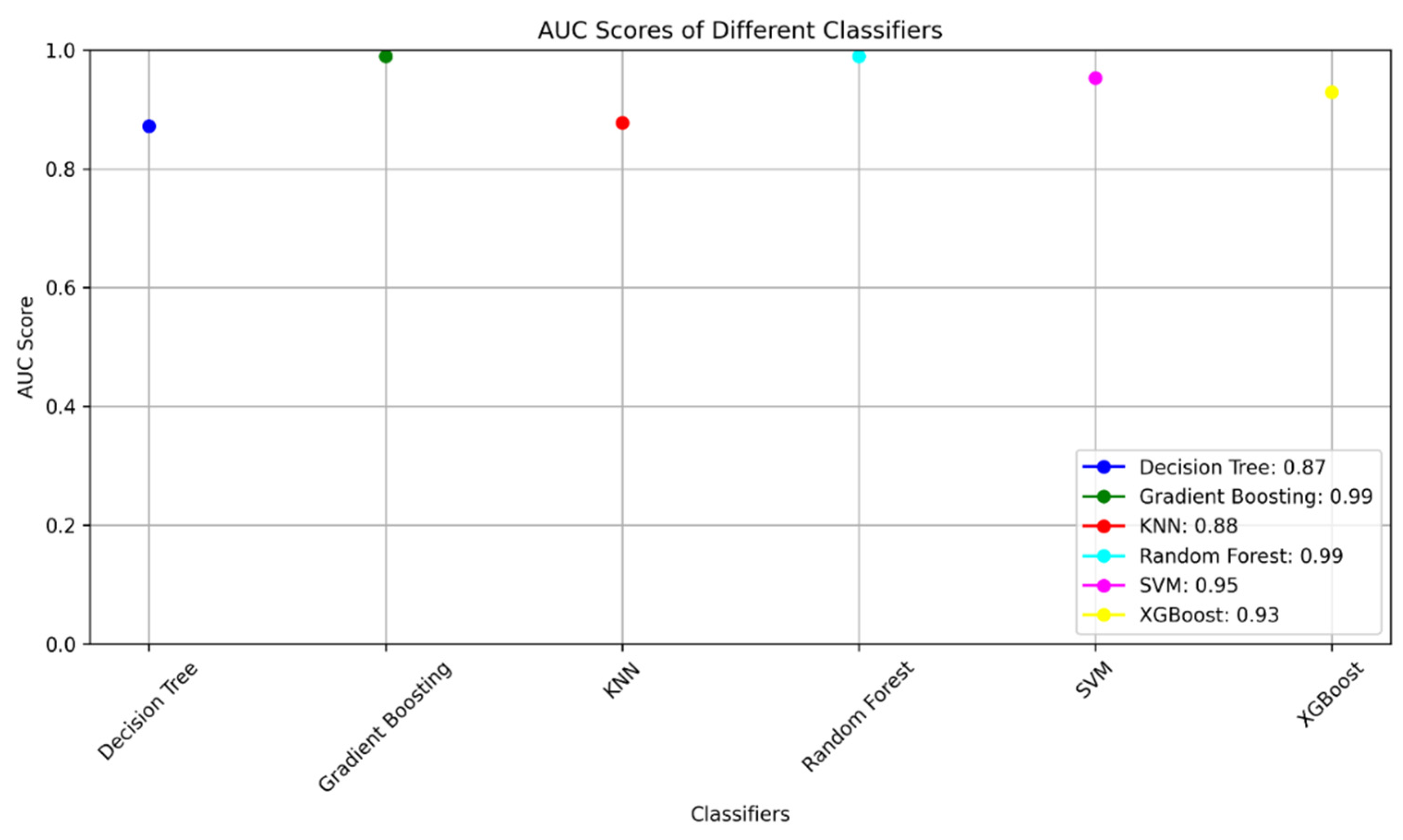
The AUC values obtained for predicting water quality index using various machine learning models provide insights into the efficacy of each model in discriminating between different water quality classes (Table 4 and Figure 5). A Decision Tree (DT) with an AUC of 0.81 indicates reasonable discriminatory power, while Random Forest (RF) and XGBoost models exhibit high AUC values of 0.94 and 0.95, respectively, reflecting their strong performance in accurately categorizing water quality. Gradient Boosting also demonstrates excellent discriminatory power with an AUC of 0.95. Support Vector Machine (SVM) performs admirably with an AUC of 0.93, suggesting effective classification. K-Nearest Neighbors (KNN) exhibits good discriminatory power, though not as high as some other models, with an AUC of 0.84. These AUC values collectively highlight the varying degrees of effectiveness among the models, emphasizing the importance of choosing models with superior discriminatory capabilities when predicting water quality index for informed decision-making in environmental management.

3.2. Statistical Analysis using Friedman Test

The Friedman Test was employed to assess the overall performance variation among multiple machine learning algorithms utilized for predicting the Water Quality Index (WQI) in the Mirpurkhas region of Sindh, Pakistan. The computed Friedman Test statistic yielded an F-value of 5.0 with a corresponding p-value of 0.4159 [53]. This analysis examines whether there exists a statistically significant difference in the performance of the various machine learning models employed for water quality assessment. The obtained p-value of 0.4159, exceeding the conventional significance level of 0.05, indicates insufficient evidence to reject the null hypothesis. Therefore, based on this statistical test, there appears to be no significant difference observed in the predictive performance of the machine learning algorithms utilized for WQI prediction in the Mirpurkhas region [54].
Table 5. The table presents the results of the Friedman Test, indicating an F-value of 5.0 and a corresponding p-value of 0.4159.
Test Value
Friedman Test - F-value 5.0
Friedman Test - p-value 0.4159

3.3. Nemenyi Test for pairwise comparisons

Each value in the matrix represents the critical distance between pairs of algorithms. In this matrix [55]: Rows and columns correspond to the XGB Classifier, Random Forest Classifier, Support Vector Classifier, K Neighbors Classifier, Gradient Boosting Classifier, Decision Tree Classifier respectively (labeled 1 to 6). The value of 1.0 along the diagonal signifies the comparison of an algorithm with itself, showing a critical distance of zero (as expected). The NaN (Not a Number) values outside the diagonal indicate that there is no significant difference between those pairs of algorithms based on the Nemenyi Test at a specific significance level.
The critical distance values are used in post-hoc tests like the Nemenyi Test to compare the average ranks of different algorithms and determine which pairs of algorithms exhibit statistically significant differences in performance [56]. If the difference in the average ranks of two algorithms exceeds the critical distance value, it suggests a statistically significant difference in their performance.
Table 6. The table illustrates the critical distance values obtained from the Nemenyi Test for pairwise comparisons among six machine learning classifiers (XGB Classifier, Random Forest Classifier, Support Vector Classifier, K Neighbors Classifier, Gradient Boosting Classifier, Decision Tree Classifier ).
XGB Classifier Random Forest Classifier Support Vector Classifier K Neighbors Classifier Gradient Boosting Classifier Decision Tree Classifier
1 1.0 NaN NaN NaN NaN NaN
2 NaN 1.0 NaN NaN NaN NaN
3 NaN NaN 1.0 NaN NaN NaN
4 NaN NaN NaN 1.0 NaN NaN
5 NaN NaN NaN NaN 1.0 NaN
6 NaN NaN NaN NaN NaN 1.0

3.3. Confusion matrix

A confusion matrix serves as a tabular tool employed in machine learning and classification endeavors to assess the efficacy of a classification algorithm. It condenses the model's predictions on a dataset, contrasting them with the actual labels [57]. This matrix proves instrumental in discerning the nature of errors made by a model, including instances of false positives and false negatives. Tables 1 through 6 in our study showcase the confusion matrices for all machine learning algorithms utilized, offering a comprehensive overview of their performance.
Table 7. The table represents a confusion matrix detailing the classification results for a multi-class classification for XGB Classifier.
True\Predicted Class 1 Class 2 Class 3 Class 4 Class 5
Class 1 2 (TP) 3 (FN) 0 0 0
Class 2 0 3 (TP) 0 1 (FP) 0
Class 3 0 3 (FP) 1 (TP) 2 (FP) 1 (TN)
Class 4 0 2 (FP) 0 1 (TP) 1 (TN)
Class 5 0 0 0 2 (FP) 62 (TP)
Table 8. The table represents a confusion matrix detailing the classification results for a multi-class classification for Random Forest Classifier.
True\Predicted Class 1 Class 2 Class 3 Class 4 Class 5
Class 1 4 (TP) 1 (FN) 0 0 0
Class 2 2 (FP) 1 (TP) 0 0 1 (FN)
Class 3 0 1 (FP) 1 (TP) 2 (FP) 3 (TN)
Class 4 0 1 (FP) 0 0 3 (TN)
Class 5 0 0 0 0 64 (TP)
Table 9. The table represents a confusion matrix detailing the classification results for a multi-class classification for SVC (Support Vector Classifier with probability=True).
True\Predicted Class 1 Class 2 Class 3 Class 4 Class 5
Class 1 4 (TP) 1 (FN) 0 0 0
Class 2 2 (FP) 1 (TP) 0 0 1 (FN)
Class 3 1 (FP) 0 0 0 6 (FN)
Class 4 0 0 0 0 4 (FN)
Class 5 0 0 0 0 64 (TP)
Table 10. The table represents a confusion matrix detailing the classification results for a multi-class classification for KNN classifier.
True\Predicted Class 1 Class 2 Class 3 Class 4 Class 5
Class 1 3 (TP) 2 (FN) 0 0 0
Class 2 3 (TP) 0 0 0 1 (FN)
Class 3 0 2 (FP) 1 (TP) 1 (FP) 3 (TN)
Class 4 0 0 0 0 4 (TN)
Class 5 0 1 (FP) 1 (TP) 2 (FP) 60 (TP)
Table 11. The table represents a confusion matrix detailing the classification results for a multi-class classification for Gradient Boosting Classifier.
True\Predicted Class 1 Class 2 Class 3 Class 4 Class 5
Class 1 4 (TP) 1 (FN) 0 0 0
Class 2 2 (FP) 1 (TP) 0 1 (FP) 0
Class 3 0 2 (FP) 2 (TP) 2 (FP) 1 (TN)
Class 4 0 2 (FP) 0 1 (TP) 1 (TN)
Class 5 0 0 0 0 64 (TP)
Table 12. The table represents a confusion matrix detailing the classification results for a multi-class classification for Decision Tree Classifier.
True\Predicted Class 1 Class 2 Class 3 Class 4 Class 5
Class 1 4 (TP) 1 (FN) 0 0 0
Class 2 2 (FP) 2 (TP) 0 0 0
Class 3 0 1 (FP) 4 (TP) 1 (FP) 1 (TN)
Class 4 0 1 (FP) 1 (FP) 1 (TP) 1 (TN)
Class 5 0 1 (FP) 1 (FP) 2 (FP) 60 (TP)
These tables exhibit the counts of true positives (TP), false positives (FP), false negatives (FN), and true negatives (TN) for each class predicted by each respective classifier in a 5-class classification problem for predicting the Water Quality Index (WQI) in the specified region.
Table 13. the table represent the water quality ranges and it’s corresponding classes.
Classes WQI Range Water Quality
Class 1 0-25 Excellent water quality
Class 2 26-50 Good water quality
Class 3 51-75 Fair water quality
Class 4 76-100 Poor water quality
Class 5 Above 100 Very poor to unacceptable water quality
Total count of class 5 instances among all classifiers:
62 + 64 + 64 + 60 + 64 + 60 = 374
Calculating the percentage of WQI values that belong to class 5:
P e r c e n t a g e   o f   C l a s s   5   W Q I = T o t a l   c o u n t   o f   i n s t a n c e s C o u n t   o f   C l a s s   5   i n s t a n c e s × 100
P e r c e n t a g e   o f   C l a s s   5   W Q I = 374 422 × 100 88.63 %
Approximately 88.63% of the Water Quality Index (WQI) values fall into class 5, which represents very poor to unacceptable water quality.
Figure 6. Testing sample result for RF classifier.
Preprints 98939 g006

4. Discussion and conclusion

In conclusion, this study harnessed the power of machine learning classifiers to predict the Water Quality Index (WQI) for the Mirpurkhas region in Sindh, Pakistan, unraveling the significance of model structures and variable importance. Notably, XGBoost and Gradient Boosting emerged as stellar performers, surpassing other models with impressive accuracy rates of 95%, while RandomForest closely followed suit, showcasing its effectiveness in WQI prediction for the region.
An additional layer of insight was gained through an uncertainty analysis, employing the R-factor to assess the reliability and consistency of predictions across the machine learning classifiers. The Information Gain (IG) analysis shed light on the pivotal role of physiochemical variables in WQI prediction, with certain variables, including 'Nitrate (NO3-N)', 'Calcium', and 'Sodium', exhibiting significant influence on water quality assessment. The prominence of specific variables underscores the critical importance of targeted monitoring and management for parameters such as 'Nitrate (NO3-N)', 'Calcium', and 'Sodium' to maintain or improve water quality standards in Mirpurkhas. The study not only demonstrates the potential of machine learning for rapid and accurate water quality assessment but also emphasizes the need to consider uncertainties associated with predictions.
Despite the promising results, limitations such as dataset size and variable scope were acknowledged, prompting recommendations for future research to include more diverse data and additional water quality parameters. Advanced strategies, including feature engineering, ensemble methods, remote sensing integration, real-time monitoring systems, and hybrid models, were proposed to enhance predictive accuracy and provide a more nuanced understanding of water quality dynamics in the region. In essence, this study not only highlights the effectiveness of machine learning in predicting WQI but also acknowledges the critical role of certain variables in water quality assessment. The incorporation of an uncertainty analysis using the R-factor adds a layer of confidence in the reliability of predictions, contributing to informed decision-making for water resource management in the Mirpurkhas region and serving as a valuable foundation for future research endeavors.

References

  1. Rao, E.P.; Puttanna, K.; Sooryanarayana, K.; Biswas, A.; Arunkumar, J. Assessment of nitrate threat to water quality in India. In The Indian nitrogen assessment; Elsevier, 2017; pp. 323–333. [Google Scholar] [CrossRef]
  2. Wanke, H.; Nakwafila, A.; Hamutoko, J.; Lohe, C.; Neumbo, F.; Petrus, I.; David, A.; Beukes, H.; Masule, N.; Quinger, M. Hand dug wells in Namibia: an underestimated water source or a threat to human health? Physics and Chemistry of the Earth, Parts A/B/C 2014, 76, 104–113. [Google Scholar] [CrossRef]
  3. Brown, T.C.; Froemke, P. Nationwide assessment of nonpoint source threats to water quality. BioScience 2012, 62, 136–146. [Google Scholar] [CrossRef]
  4. Lapworth, D.; Boving, T.; Kreamer, D.; Kebede, S.; Smedley, P. Groundwater quality: Global threats, opportunities and realising the potential of groundwater. 2022, 811, 152471. [Google Scholar] [CrossRef] [PubMed]
  5. Memon, A.H.; Lund, G.M.; Channa, N.A.; Younis, M.; Ali, S.; Shah, F.B. Analytical Study of Drinking Water Quality Sources of Dighri Sub-division of Sindh, Pakistan. 2016. [Google Scholar]
  6. Khan, S.; Aziz, T.; Noor-Ul-Ain, A.K.; Ahmed, I.; Nida, A. Drinking water quality in 13 different districts of Sindh, Pakistan. Health Care Curr Rev 2018, 6, 1000235. [Google Scholar] [CrossRef]
  7. Akhan, F.; Siddqui, I.; USMANI, T. of Larkana and Mirpurkhas Districts of Sind. Jour. Chem. Soc. Pak. Vol 2006, 28, 131. [Google Scholar]
  8. Hayder, G.; Kurniawan, I.; Mustafa, H.M. Implementation of machine learning methods for monitoring and predicting water quality parameters. Biointerface Res. Appl. Chem 2020, 11, 9285–9295. [Google Scholar] [CrossRef]
  9. Avila, R.; Horn, B.; Moriarty, E.; Hodson, R.; Moltchanova, E. Evaluating statistical model performance in water quality prediction. Journal of environmental management 2018, 206, 910–919. [Google Scholar] [CrossRef] [PubMed]
  10. Ashwini, K.; Vedha, J.; Priya, M. Intelligent model for predicting water quality. Int. J. Adv. Res. Ideas Innov. Technol. ISSN 2019, 5, 70–75. [Google Scholar]
  11. Kalin, L.; Isik, S.; Schoonover, J.E.; Lockaby, B.G. Predicting water quality in unmonitored watersheds using artificial neural networks. Journal of environmental quality 2010, 39, 1429–1440. [Google Scholar] [CrossRef]
  12. McGrane, S.J. Impacts of urbanisation on hydrological and water quality dynamics, and urban water management: a review. Hydrological Sciences Journal 2016, 61, 2295–2311. [Google Scholar] [CrossRef]
  13. Dutt, V.; Sharma, N. Potable water quality assessment of traditionally used springs in a hilly town of Bhaderwah, Jammu and Kashmir, India. Environmental monitoring and assessment 2022, 194, 30. [Google Scholar] [CrossRef] [PubMed]
  14. Lermontov, A.; Yokoyama, L.; Lermontov, M.; Machado, M.A.S. River quality analysis using fuzzy water quality index: Ribeira do Iguape river watershed, Brazil. Ecological Indicators 2009, 9, 1188–1197. [Google Scholar] [CrossRef]
  15. De Pauw, N.; Vanhooren, G. Method for biological quality assessment of watercourses in Belgium. Hydrobiologia 1983, 100, 153–168. [Google Scholar] [CrossRef]
  16. Zhang, Y.; Guo, F.; Meng, W.; Wang, X.-Q. Water quality assessment and source identification of Daliao river basin using multivariate statistical methods. Environmental monitoring and assessment 2009, 152, 105–121. [Google Scholar] [CrossRef]
  17. Lenat, D.R. Water quality assessment of streams using a qualitative collection method for benthic macroinvertebrates. Journal of the North American Benthological Society 1988, 7, 222–233. [Google Scholar] [CrossRef]
  18. Behmel, S.; Damour, M.; Ludwig, R.; Rodriguez, M. Water quality monitoring strategies—A review and future perspectives. Science of the Total Environment 2016, 571, 1312–1329. [Google Scholar] [CrossRef] [PubMed]
  19. Hassan, M.M.; Hassan, M.M.; Akter, L.; Rahman, M.M.; Zaman, S.; Hasib, K.M.; Jahan, N.; Smrity, R.N.; Farhana, J.; Raihan, M. Efficient prediction of water quality index (WQI) using machine learning algorithms. Human-Centric Intelligent Systems 2021, 1, 86–97. [Google Scholar] [CrossRef]
  20. Lap, B.Q.; Du Nguyen, H.; Hang, P.T.; Phi, N.Q.; Hoang, V.T.; Linh, P.G.; Hang, B.T.T. Predicting water quality index (WQI) by feature selection and machine learning: a case study of An Kim Hai irrigation system. Ecological Informatics 2023, 74, 101991. [Google Scholar] [CrossRef]
  21. Ding, F.; Zhang, W.; Cao, S.; Hao, S.; Chen, L.; Xie, X.; Li, W.; Jiang, M. Optimization of water quality index models using machine learning approaches. Water Research 2023, 243, 120337. [Google Scholar] [CrossRef] [PubMed]
  22. Van Rossum, G. Python Programming Language. In Proceedings of the USENIX annual technical conference; 2007; pp. 1–36. [Google Scholar]
  23. Saabith, A.S.; Vinothraj, T.; Fareez, M. Popular python libraries and their application domains. International Journal of Advance Engineering and Research Development 2020, 7. [Google Scholar]
  24. Bansal, S.; Ganesan, G. Advanced evaluation methodology for water quality assessment using artificial neural network approach. Water Resources Management 2019, 33, 3127–3141. [Google Scholar] [CrossRef]
  25. Gevrey, M.; Rimet, F.; Park, Y.S.; Giraudel, J.L.; Ector, L.; Lek, S. Water quality assessment using diatom assemblages and advanced modelling techniques. Freshwater biology 2004, 49, 208–220. [Google Scholar] [CrossRef]
  26. Uddin, M.G.; Olbert, A.I.; Nash, S. Assessment of water quality using Water Quality Index (WQI) models and advanced geostatistical technique. Civil Engineering Research Association of Ireland (CERAI). Civil Engineering Research Association of Ireland (CERAI), 2020; 594–599. [Google Scholar]
  27. Soomro, A.; Mangrio, M.; Bharchoond, Z.; Mari, F.; Pirzada, P.; Lashari, B.; Bhatti, M.; Skogerboe, G. Maintenance plans for irrigation facilities of pilot distributaries in Sindh Province, Pakistan. Volume 3-Bareji Distributary, Mirpurkhas District; IWMI, 1997. [Google Scholar]
  28. Van der Hoek, W.; Boelee, E.; Konradsen, F. Irrigation, domestic water supply and human health; Encyclopedia of Life Support Systems (EOLSS): Paris, France, 2002. [Google Scholar]
  29. Van der Hoek, W.; Konradsen, F.; Ensink, J.H.; Mudasser, M.; Jensen, P.K. Irrigation water as a source of drinking water: is safe use possible? Tropical medicine & international health 2001, 6, 46–54. [Google Scholar] [CrossRef]
  30. Akhtar, N.; Syakir Ishak, M.I.; Bhawani, S.A.; Umar, K. Various natural and anthropogenic factors responsible for water quality degradation: A review. Water 2021, 13, 2660. [Google Scholar] [CrossRef]
  31. Khatri, N.; Tyagi, S. Influences of natural and anthropogenic factors on surface and groundwater quality in rural and urban areas. Frontiers in life science 2015, 8, 23–39. [Google Scholar] [CrossRef]
  32. Burri, N.M.; Weatherl, R.; Moeck, C.; Schirmer, M. A review of threats to groundwater quality in the anthropocene. Science of the Total Environment 2019, 684, 136–154. [Google Scholar] [CrossRef]
  33. Udhayakumar, R.; Manivannan, P.; Raghu, K.; Vaideki, S. Assessment of physico-chemical characteristics of water in Tamilnadu. Ecotoxicology and environmental safety 2016, 134, 474–477. [Google Scholar] [CrossRef]
  34. Patil, P.; Sawant, D.; Deshmukh, R. Physico-chemical parameters for testing of water–A review. International journal of environmental sciences 2012, 3, 1194–1207. [Google Scholar]
  35. Brusseau, M.; Walker, D.; Fitzsimmons, K. Physical-chemical characteristics of water. In Environmental and pollution science; Elsevier, 2019; pp. 23–45. [Google Scholar] [CrossRef]
  36. Kroll, C.N.; Song, P. Impact of multicollinearity on small sample hydrologic regression models. Water Resources Research 2013, 49, 3756–3769. [Google Scholar] [CrossRef]
  37. Sulaiman, M.S.; Abood, M.M.; Sinnakaudan, S.K.; Shukor, M.R.; You, G.Q.; Chung, X.Z. Assessing and solving multicollinearity in sediment transport prediction models using principal component analysis. ISH Journal of Hydraulic Engineering 2021, 27, 343–353. [Google Scholar] [CrossRef]
  38. Iliou, T.; Anagnostopoulos, C.-N.; Nerantzaki, M.; Anastassopoulos, G. A novel machine learning data preprocessing method for enhancing classification algorithms performance. In Proceedings of the Proceedings of the 16th International Conference on Engineering Applications of Neural Networks (INNS), 2015; Nerantzaki, M., Ed.; pp. 1–5. [CrossRef]
  39. Werner de Vargas, V.; Schneider Aranda, J.A.; dos Santos Costa, R.; da Silva Pereira, P.R.; Victória Barbosa, J.L. Imbalanced data preprocessing techniques for machine learning: a systematic mapping study. Knowledge and Information Systems 2023, 65, 31–57. [Google Scholar] [CrossRef]
  40. Veček, N.; Črepinšek, M.; Mernik, M. On the influence of the number of algorithms, problems, and independent runs in the comparison of evolutionary algorithms. Applied Soft Computing 2017, 54, 23–45. [Google Scholar] [CrossRef]
  41. Liang, G.; Zhang, C. A comparative study of sampling methods and algorithms for imbalanced time series classification. In Proceedings of the AI 2012: Advances in Artificial Intelligence: 25th Australasian Joint Conference, Sydney, Australia, 4-7 December 2012; Proceedings 25, 2012. pp. 637–648. [Google Scholar] [CrossRef]
  42. Browne, M.W. Cross-validation methods. Journal of mathematical psychology 2000, 44, 108–132. [Google Scholar] [CrossRef]
  43. Daoud, J.I. Multicollinearity and regression analysis. In Proceedings of the Journal of Physics: Conference Series; 2017; p. 012009. [Google Scholar] [CrossRef]
  44. Akram, P.; Solangi, G.S.; Shehzad, F.R.; Ahmed, A. Groundwater Quality Assessment using a Water Quality Index (WQI) in Nine Major Cities of Sindh, Pakistan. International Journal of Research in Environmental Science (IJRES) 2020, 6, 18–26. [Google Scholar] [CrossRef]
  45. Wijaya, D.R.; Sarno, R.; Zulaika, E. Information Quality Ratio as a novel metric for mother wavelet selection. Chemometrics and Intelligent Laboratory Systems 2017, 160, 59–71. [Google Scholar] [CrossRef]
  46. Singhee, A.; Rutenbar, R.A. Why quasi-Monte Carlo is better than Monte Carlo or Latin hypercube sampling for statistical circuit analysis. IEEE Transactions on Computer-Aided Design of Integrated Circuits and Systems 2010, 29, 1763–1776. [Google Scholar] [CrossRef]
  47. Hoffman, R.N.; Kalnay, E. Lagged average forecasting, an alternative to Monte Carlo forecasting. Tellus A: Dynamic Meteorology and Oceanography 1983, 35, 100–118. [Google Scholar] [CrossRef]
  48. Feroz, F.; Hobson, M.P. Multimodal nested sampling: an efficient and robust alternative to Markov Chain Monte Carlo methods for astronomical data analyses. Monthly Notices of the Royal Astronomical Society 2008, 384, 449–463. [Google Scholar] [CrossRef]
  49. Noori, R.; Karbassi, A.; Moghaddamnia, A.; Han, D.; Zokaei-Ashtiani, M.; Farokhnia, A.; Gousheh, M.G. Assessment of input variables determination on the SVM model performance using PCA, Gamma test, and forward selection techniques for monthly stream flow prediction. Journal of hydrology 2011, 401, 177–189. [Google Scholar] [CrossRef]
  50. Pan, M.; Li, C.; Liao, J.; Lei, H.; Pan, C.; Meng, X.; Huang, H. Design and modeling of PEM fuel cell based on different flow fields. Energy 2020, 207, 118331. [Google Scholar] [CrossRef]
  51. Pirmohamed, M.; Burnside, G.; Eriksson, N.; Jorgensen, A.L.; Toh, C.H.; Nicholson, T.; Kesteven, P.; Christersson, C.; Wahlström, B.; Stafberg, C. A randomized trial of genotype-guided dosing of warfarin. New England Journal of Medicine 2013, 369, 2294–2303. [Google Scholar] [CrossRef]
  52. Sharafati, A.; Yasa, R.; Azamathulla, H.M. Assessment of stochastic approaches in prediction of wave-induced pipeline scour depth. Journal of Pipeline Systems Engineering and Practice 2018, 9, 04018024. [Google Scholar] [CrossRef]
  53. Sheldon, M.R.; Fillyaw, M.J.; Thompson, W.D. The use and interpretation of the Friedman test in the analysis of ordinal-scale data in repeated measures designs. Physiotherapy Research International 1996, 1, 221–228. [Google Scholar] [CrossRef] [PubMed]
  54. Pereira, D.G.; Afonso, A.; Medeiros, F.M. Overview of Friedman’s test and post-hoc analysis. Communications in Statistics-Simulation and Computation 2015, 44, 2636–2653. [Google Scholar] [CrossRef]
  55. Pohlert, T. The pairwise multiple comparison of mean ranks package (PMCMR). R package 2014, 27, 9. [Google Scholar]
  56. Garcia, S.; Herrera, F. An Extension on" Statistical Comparisons of Classifiers over Multiple Data Sets" for all Pairwise Comparisons. Journal of machine learning research 2008, 9. [Google Scholar]
  57. Townsend, J.T. Theoretical analysis of an alphabetic confusion matrix. Perception & Psychophysics 1971, 9, 40–50. [Google Scholar] [CrossRef]
Figure 3. Input parameter used for water quality index prediction and assessment.
Preprints 98939 g003
Figure 4. Predicted values, along with the prediction intervals using bootstrapping.
Preprints 98939 g004
Figure 5. The AUC score for different classifiers used for water quality index prediction and assessment.
Preprints 98939 g005
Table 3. R-factor obtain for all the machine Learning Algorithms in WQI Prediction.
Classifier R-factor
K-Nearest Neighbors 0.83
Decision Tree 0.77
Gradient Boosting 0.83
Random Forest 0.83
SVM 0.83
XGBoost 0.83
Table 4. Performance Evaluation of Machine Learning Algorithms in WQI Prediction.
Algorithm AUC
Decision Tree (DT) 0.81
Random Forest (RF) 0.94
Gradient Boosting 0.95
K-Nearest Neighbors (KNN) 0.84
Support Vector Machine (SVM) 0.93
XGBoost 0.95
Disclaimer/Publisher’s Note: The statements, opinions and data contained in all publications are solely those of the individual author(s) and contributor(s) and not of MDPI and/or the editor(s). MDPI and/or the editor(s) disclaim responsibility for any injury to people or property resulting from any ideas, methods, instructions or products referred to in the content.
Copyright: This open access article is published under a Creative Commons CC BY 4.0 license, which permit the free download, distribution, and reuse, provided that the author and preprint are cited in any reuse.
Alerts
Prerpints.org logo

Preprints.org is a free preprint server supported by MDPI in Basel, Switzerland.

Subscribe

© 2025 MDPI (Basel, Switzerland) unless otherwise stated