Kullback-Leibler Divergence(KLD) Formalism of The Stable Queue with KLD Applications to Biometrics

Preprint

Article

Kullback-Leibler Divergence(KLD) Formalism of The Stable Queue with KLD Applications to Biometrics

This version is not peer-reviewed.

Dr Ismail A Mageed^*

This version is not peer-reviewed.

Altmetrics

Downloads

Views

Comments

Submitted:

17 February 2024

Posted:

19 February 2024

You are already at the latest version

Abstract

The paper explores the Kullback-Leibler divergence formalism (KLDF) applied to the stable MG1 queue manifold. More potentially, both service time probability and cumulative functions which make KLDF exact are obtained. The credibility of KLDF is justified through consistency axioms. Some potential applications of Kullback-Leibler divergence to Biometry are presented. The paper concludes with closing remarks combined with some challenging open problems and the next phase of research.

Keywords:

Subject:

Computer Science and Mathematics - Probability and Statistics

I. Introduction

It has been common practice in probabilistic inverse approaches [1] to treat both measurable data and model parameters that are unknown as uncertain. This method provides deeper understanding of the uncertainty associated with the measured data and model parameters. [2–10]. KLD [11–16] is a method used to compare two probability distributions. In Probability and Statistics, when we need to simplify complex distributions or approximate observed data, KL Divergence helps us quantify the amount of information lost in the process of choosing an approximation. KLD measures the difference between the two distributions and assists us with comprehending the trade-off between accuracy and simplicity in statistical modelling.

Shannonian entropic measure [9,17], namely H(p) reads as

H (p) = - \sum_{n = 0}^{\infty} p (n) l n (p (n))

(1)

to define “The minimum number of bits it would take us to encode our information”.

KLD is commonly written as:

D_{K L} (p | | r = \sum_{n = 0}^{\infty} p (n) l n \frac{p (n)}{r (n)}

We can precisely quantify lost when approximating one distribution with another using KL divergence.

This paper provides a roadmap of its contents, starting with some fundamental background in section I. The main results are given in section II. Section III deals with potential KLD applications to Biometrics. Finally, section IV provides conclusions, some emerging open problems, and future pathways of research.

According to [18–20], the maximum entropy state probability of the generalized geometric solution of a stable M/G/1 queue, subject to normalization, mean queue length (MQL), L and server utilization,

ρ

(<1) is given by:

Figure 1. A Stable M/G/1 queue.

p (n) = \{\begin{matrix} 1 - ρ, n = 0 \\ (1 - ρ) g x^{n}, n \geq 1 \end{matrix}

(3)

where

g = \frac{ρ^{2}}{(L - ρ) (1 - ρ)}, x = \frac{L - ρ}{L}

and

L = \frac{ρ}{2} (1 + \frac{1 + ρ C_{s}^{2}}{1 - ρ})

(MQL for the underlying queue),

ρ

(= 1 -

p (0))

and

C_{s}^{2}

is the squared coefficient of variations

) .

Obviously,

p (n)

(c.f., (3)) reads:

p (n) = \{\begin{matrix} 1 - ρ, n = 0 \\ \frac{2 ρ {(\frac{1 + ρ β}{1 - ρ} - 1)}^{n - 1}}{({(\frac{1 + ρ β}{1 - ρ} + 1)}^{n}}, n \geq 1 \end{matrix}

(4)

where

β = C_{s}^{2} .

The reader can observe the difference between our novel approach and that in (3) and (4). Moreover, it is notable that the newly obtained KL formalism in the current paper is more general which reduces to (3) as a special case.

[19] evaluated the credibility of Tsallis’ NME formalism in terms of the four consistency axioms for large systems.

The credibility of KLDF NME formalism as a method of inductive reasoning is in Appendix A.

It has been shown (c.f., [19]) that the EME state steady probability of a stable M/G/1 queue that maximizes Shannon’s entropy function (c.f., [17]),

H (p_{1, S}) = - \sum_{n = 0}^{\infty} p (n) \ln (p (n))

(5)

with requirements,

Normalization,

\sum_{n = 0}^{\infty} p (n) = 1

(6)

SU,

p_{1, S} (0) = \sum_{n = 0}^{\infty} h (n) p (n) = 1 - ρ, ρ = \frac{λ}{μ}

(7)

where

h (n) = 1 for n = 0 and h (n) = 0 for n = 1, 2, \dots .

(8)

P-K MQL,

< n > = \sum_{n = 0}^{\infty} n p (n) = \frac{ρ}{2} (1 + \frac{1 + ρ C_{s}^{2}}{1 - ρ})

(6)

reads

p (n) = \{\begin{matrix} p (0), n = 0 \\ p (0) τ_{s} x^{n} n > 0 \end{matrix}

(10)

where

p (0) = 1 - ρ, τ_{s}

= 2/(1+

C_{s}^{2}

) and

x = \frac{< n > - ρ}{< n >} .

II. MAIN RESULTS

Theorem 1. KLDF, namely,

p_{K L} (n),

under (6)-(9) reads as

p_{K L} (n) = \{\begin{matrix} p_{K L} (0) n = 0 \\ \frac{p_{K L} (0) τ_{s} y^{n}}{q (0)} n > 0 \end{matrix}

(11, KL)

where the initial state probabilities

p_{K L} (0)

satisfy the SU constraint (6)

p_{K L} (0) = 1 - ρ

(12)

Such that

τ_{s} = 2 / (1 + C_{s}^{2})

(13)

y = \frac{< n > - ρ}{< n >} = \frac{ρ}{ρ + {{(τ}_{K L}) p}_{K L} (0)},

y^{n} = {q (n) x}^{n}, M Q L = < n > = \frac{ρ}{2} (1 + \frac{ρ C_{s, K L}^{2}}{1 - ρ})

(14)

with

\frac{ρ (1 - y)}{(1 - ρ) y} = \frac{τ_{s}}{q (0)} = τ_{K L} (15)

(15)

Proof

The Lagrangian, follows by maximizing KLDF under (6)-(9) to satisfy:

[\sum_{n = 0}^{\infty} p_{K L} (n) \ln (\frac{p_{K L} (n)}{q (n)}) - α (\sum_{n = 0}^{\infty} h (n)) + (β - 1) (\sum_{n = 0}^{\infty} 1) - γ (\sum_{n = 0}^{\infty} n) = 0

(16)

Hence,

\ln (\frac{p_{K L} (n)}{q (n)}) + 1 + (β - 1) - α h (n) + γ n = 0

Hence

p_{K L} (n) = q (n) {(e}^{- β}) {(e}^{α h (n)}) {(e}^{- γ n})

(17)

n = 0, (17)

translates to

p_{K L} (0) = q (0) {(e}^{- β}) {(e}^{α})

(18)

Linking (17) with (18) implies

p_{K L} (n) = \frac{p_{K L} (0) q (n) τ_{s} x^{n}}{q (0)},

x = e^{- γ} \in (0,1), τ_{s} = e^{- α} \in (0,1)

(19)

Hence, we have

Define,

y^{n} = {q (n) x}^{n}, y = \frac{< n > - ρ}{< n >},

implies that

p_{K L} (n)

will get the form:

p_{K l} (n) = \{\begin{matrix} p_{K L} (0) n = 0 \\ \frac{p_{K L} (0) τ_{s} y^{n}}{q (0)} n > 0 \end{matrix}

(20, KL)

Thus

1 = p_{K L} (0) + p_{K L} (0) τ_{s} \frac{y}{(1 - y) q (0)}

, implying

\frac{ρ (1 - y)}{(1 - ρ) y} = τ_{K L},

which clearly implies

y = \frac{ρ}{ρ + {{(τ}_{K l}) p}_{K L} (0)}

. This proves the required results.

Clearly, from the above devised result

p_{K L} (n) = \{\begin{matrix} p_{K L} (0) n = 0 \\ \frac{p_{K L} (0) τ_{s} y^{n}}{q (0)} n > 0 \end{matrix}

(20, KI)

It is known that

q (0) \in (0,1

). it is evident that as

q (0) \to 1,

the KL formalism in (20,KL) will get the form:

p_{S h} (n) = \{\begin{matrix} p_{K L} (0) n = 0 \\ p_{K L} (0) τ_{s} y^{n} n > 0 \end{matrix}

which is the obtained Shannonian formalism in [20]. This shows the strength of the newly devised KLD formalism.

Theorem 2. The KL NME formalism,

p_{K L} (n),

are exact when PDFs of service time read as

f_{s, K L} (t) = (1 - τ_{K L}) u_{0} (t) + μ {(τ_{K L})}^{2} e^{- μ τ_{K L}}

(21)

where

u_{0} (t)

reads as

u_{0} (t) = \{\begin{matrix} \infty, t = 0 \\ 0, t \neq 0 \end{matrix}

(22)

such that

\int_{- \infty}^{\infty} u_{0} (t) = 1 and τ_{s} = 2 / (1 + C_{s}^{2}), τ_{K L} = \frac{τ_{s}}{q (0)}

Proof

Q_{K L} (z) (c . f ., [20])

for

p_{K L} (n) (c . f ., 20, K L)

reads as

Q_{K L} (z) = \sum_{n = 0}^{\infty} p_{K L} (n) z^{n}, |z| < 1

(23)

H e n c e,

by replacing

p_{K L} (n)

of (20,KL) into (23), we have

Q_{K L} (z) = \sum_{n = 0}^{\infty} p_{K L} (n) z^{n} =

p_{K L} (0) + \frac{p_{K L} (0) τ_{K L} y z}{(1 - y z)} = \frac{p_{K l} (0) (1 - y z (1 - τ_{K L}))}{1 - y z}

(24)

Following [21],

Q_{K l} (z) = \frac{p_{K L} (0) (1 - z) (F_{s, K L}^{*} (λ - λ z))}{F_{s, K L}^{*} (λ - λ z) - z}

(25)

where

F_{s, K l}^{*} (θ) = E [e^{- θ s}] = \int_{0}^{\infty} e^{- θ t} f_{s, K l} (t) d t

(26)

Hence,

\frac{(1 - z) (F_{s, K L}^{*} (λ - λ z))}{F_{s, K L}^{*} (λ - λ z) - z} = \frac{(1 - y z (1 - τ_{K L}))}{1 - y z}

(27)

Following (27), yields

F_{s, K L}^{*} (λ - λ z) = \frac{z ((1 - y z (1 - τ_{K L}))}{((1 - y z (1 - τ_{K L})) - (1 - z) (1 - y z))} = \frac{(1 - y z (1 - τ_{K L}))}{y τ_{K L} - y z + 1}

(28)

Define,

λ - λ z = θ

. Therefore,

z = 1 - \frac{θ}{λ}

(29)

Thus,

F_{s, K L}^{*} (θ) = \frac{μ τ_{K L} + θ (1 - τ_{K L})}{θ + μ τ_{K L}} = (1 - τ_{K L}) + \frac{μ {(τ_{K L})}^{2}}{θ + μ τ_{K L}}

(30)

By inverting Laplace-StieltjesTransform,

F_{s, K L}^{*} (θ)

the GE_Kl-type pdf

f_{s, K L} (t)

(c.f., (21)) follows.

It is observed that as

q (0) \to 1

τ_{K L} \to τ_{s}

, which reduces to the Shannonian limiting case obtained (c,f., [20]).

Corollary 1. The CDF

F_{s, K L} (t) o

f the GE_KL type of service time with the PDFs

f_{s, K L} (t)

of Theorem 2 is captured fully by

F_{s, K l} (t)}

, which reads as

F_{s, K L} (t) = 1 - τ_{K L} e^{- μ τ_{K L} t}

τ_{s}

= 2/(1+

C_{s,}^{2}

τ_{K L} = \frac{τ_{s}}{q (0)} .

Proof

We have

F_{s, K L} (t)

\int_{0}^{t} f_{s, K L} (x) d x

\int_{0}^{t} (1 - τ_{K L}) u_{0} (x) d x + μ τ_{K L} \int_{0}^{t} e^{- μ τ_{K L} x} d x = (1 - τ_{K L}) + \frac{μ τ_{K L}}{μ τ_{K L}} (1 - e^{- μ τ_{K L} t}) = 1 - τ_{K L} e^{- μ τ_{K L} t} QED

(c.f., 31)

For

q (0) \to

1, the novel derivation (31) reduces to the formula in [20],

F_{s} (t)

1 - τ_{s} e^{- τ_{s} μ t}

with

τ_{s} = \frac{2}{C_{s}^{2} + 1} .

Corollary 2. Following (21), we have

E (s_{K L}) = \frac{1}{μ}

(32)

E (s_{K L}^{2}) = \frac{2}{μ^{2} τ_{K L}}

(33)

C_{s, K L}^{2} = \frac{E (s_{K L}^{2})}{{(E (S_{K L}))}^{2}} - 1 = \frac{(2 - τ_{K L})}{τ_{K L}}

(34)

{τ_{K L} = \frac{τ_{s}}{q (0)}, τ}_{s} = 2 / (1 + C_{s}^{2})

Proof

The mean of

S_{K L}

is given by

E (S_{K L}) = \int_{0}^{\infty} t f_{s . K L} (t) d t = \int_{0}^{\infty} t μ τ_{K L} e^{- μ τ_{K L} t} d t = μ τ_{K L} \int_{0}^{\infty} t e^{- μ τ_{K L} t} d t

(35)

Introducing

Γ (m) = \int_{0}^{\infty} w^{m - 1} e^{- w} d w

(36)

and substituting

w = μ τ_{K L} t

on (35) and since

Γ (2) = 1,

it is implied that

E (s_{K L}) = \frac{μ τ_{K L}}{μ^{2} {(τ_{K L})}^{2}} Γ (2) = \frac{1}{μ} .

Moreover,

E (s_{K L}^{2}) = \int_{0}^{\infty} t^{2} f_{s, K L} (t) d t = \int_{0}^{\infty} t^{2} μ τ_{K L} e^{- μ τ_{K L} t} d t = μ τ_{K L} \int_{0}^{\infty} t^{2} e^{- μ τ_{K L} t} d t

(36)

Let

w = μ τ_{K L} t

E (s_{K L}^{2})

is given by (33). Hence

C_{s, q, R}^{2}

by (34).

q (0) \to

1, the new derivations (32)-(34) reduce to that in [20],

E (S) = \frac{1}{μ}

(37)

E (S^{2}) = \frac{2}{μ^{2} τ_{K L}}

(38)

C_{s, K L}^{2} = \frac{E (S^{2})}{{(E (S))}^{2}} - 1 = \frac{(2 - τ_{K L})}{τ_{K L}}

(39)

with

{τ_{K L} = \frac{τ_{s}}{q (0)}, τ}_{s} = 2 / (1 + C_{s}^{2}) .

III. KLD APPLICATIONS TO BIOMETRICS

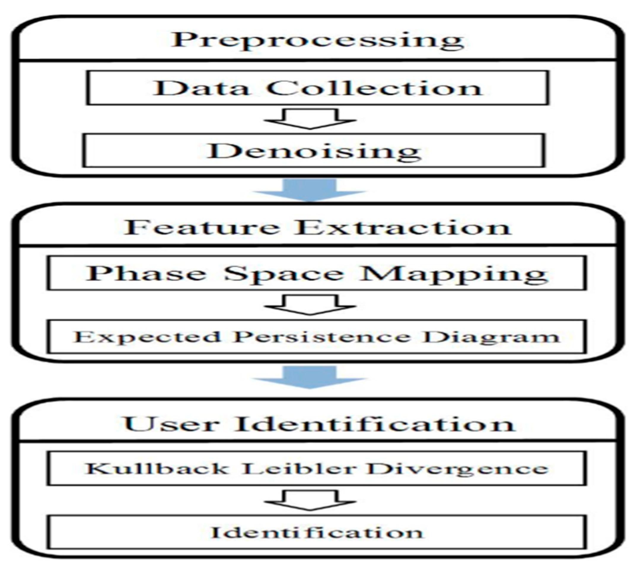
The use of biometric information was addressed by [25], specifically accelerometer data collected by smartphones, for advanced authentication and on-line user identification. The proposed approach utilizes homological analysis to monitor the inherent walking patterns of different users in the accelerometer data. By transforming the expected persistence diagrams into probability distribution functions and measuring the discrepancy in walking patterns using the KLD, users can be identified with high accuracy.

In [25] a proposed user identification system that utilizes accelerometer data was employed. The raw data is then filtered, and the magnitude of the accelerometer readings is calculated. The system focuses on identifying the user’s activity, specifically walking, by extracting the associated accelerometer data. This is illustrated by Figure 2.

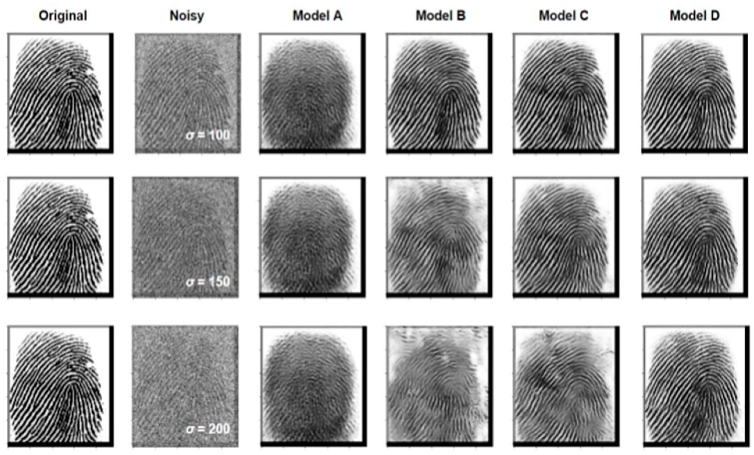
The Sokoto Coventry Fingerprint Dataset (SOCOFing) [26] was used in this study to construct and evaluate different models. SOCOFing is a biometric fingerprint database consisting of 6,000 grayscale images collected from 600 African subjects. The dataset was partitioned into training, validation, and testing sets, and four neural network architectures were trained and evaluated, with the Res-WCAE model outperforming others in terms of noise reduction and achieving state-of-the-art performance. This can be seen from Figure 3 (c.f., [26]).

To improve the ability of the proposed model [26] to make accurate predictions on unseen data, a regularized cost function that includes KLD regularization was introduced. This regularization is achieved by incorporating a prior distribution into the cost function.

Recently [27], LSR has been found to be effective in reducing the variation within a class by minimizing KLD between a uniform distribution and the predicted distribution of a neural network. This regularization method helps improve the performance of the network by providing more robust and generalized predictions, particularly in classification tasks where reducing overconfidence and overfitting are important considerations.

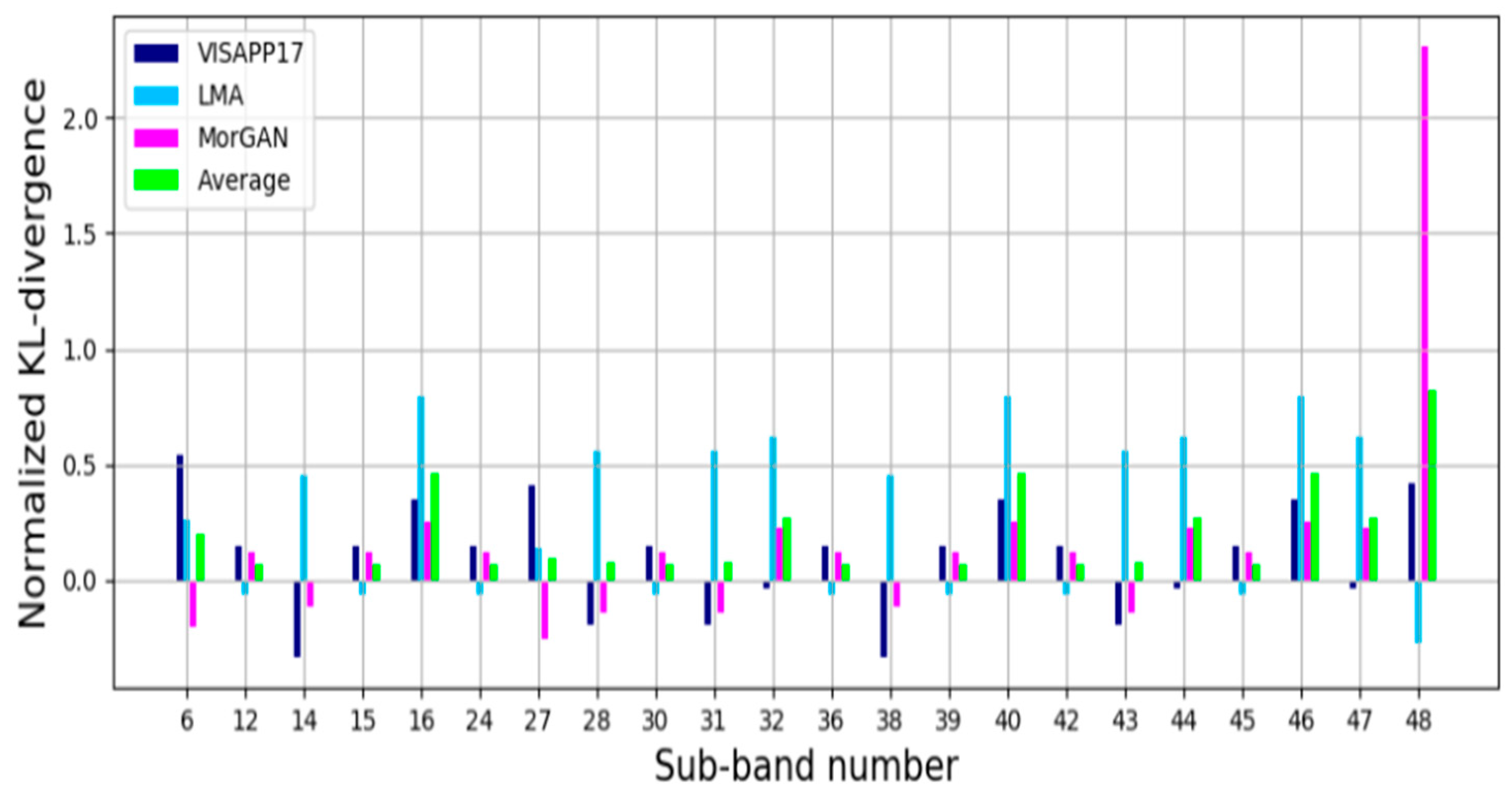
To select the most informative sub-bands [28], the KL-divergence values of each dataset are normalized and averaged across the three datasets. Higher KL-divergence values indicate more discriminative sub-bands for classification. The sub-bands are chosen based on the highest average KLD values from all datasets, allowing for the identification of sub-bands that are discriminative across different datasets, as shown by Figure (c.f., [28]).

IV. SUMMARY, RESEARCH QUESTIONS COMBINED WITH NEXT PHASE RESEARCH

The ever-challenging problem of finding the closed form expression of the KLD formalism of the stable

M / G / 1

queue is solved in this paper. More fundamentally, the corresponding service time PDF and CDF for which the derived KLDF is exact are obtained. Some potential KLD applications to Biometrics are highlighted.

These are few emerging research questions:

Can we unlock the mystery of the threshold of the obtained CDF(c.f., (31))?
A really challenging open problem is replacing the proposed KLD in this paper by the corresponding KLD for Ismail’s Entropy(IE) (c.f., [29]). This is a yet a great challenge to world mathematicians till current.
Is the open problem of finding the info-geometric analysis of the derived KLDF solvable?
Replacing the proposed version of KLD in this paper by the corresponding KLD of Ismail’s entropy(IE)[29], can we get better results to advance Biometrics?

The next phase of research includes solving the above-listed open problems.

Appendix A. KL FORMALISM VS. EME CONSISTEN-CY AXIOMS

1. Uniqueness

It translates to, “If the same problem is solved twice in exactly the same way, the same answer is expected in both cases i.e., the solution should be unique” (c.f., [6]). Let

f_{K L}, h_{K l}

be two PDFs such that:

H_{K l}^{*} (f_{K L, N}) = H_{K}^{*} (h_{K L, N})

(A.1)

Hence,

\sum_{n = 1}^{N} (f_{K L, N}) l n (\frac{(f_{K L, N})}{q (N)}) = \sum_{n = 1}^{N} (h_{K L, n}) l n (\frac{(h_{K L, N})}{q (N)})

(A.2)

By (A.2),it is implied that:

(f_{K L, N}) (l n (f_{K L, N}) - l n (q (N))) = (h_{K L, N}) (l n (h_{K L, N}) - l n (q (N)))

(A.3)

Let the contradiction be true, namely,

(f_{K L, N}) \neq (h_{K L, N})

. Thus

\exists γ > 1

satisfying:

(f_{K L, N}) = γ (h_{K L, N})

(A.4)

Combining (A.3) and (A.4), we get

γ (h_{K L, N}) (l n γ + l n (h_{K L, N}) - l n (q (N)) = (h_{K L, N}) (l n (h_{K L, N}) - l n (q (N))

(A.5)

Since

(h_{K L, N})

is non-zero, (A.5) can be transformed into

γ (l n γ) = (1 - γ) (l n (\frac{(h_{K L, N})}{q (N)})

(A.6)

By default,

q (N) \in (0,1)

By mathematical analysis, we have the following possibilities:

(1): $q (N) <$ $h_{K L, N}$

It is implied that $\frac{(h_{K L, N})}{q (N)} > 1$ , ln( $\frac{(h_{K L, N})}{q (N)}) > 0$ .

This implies by (A.6), $γ > 1,$ that $γ (l n γ) < 0$ (Contradiction)
(2): $q (N) =$ $h_{K L, N}$

It is implied that $\frac{(h_{K L, N})}{q (N)} = 1$ , ln( $\frac{(h_{K L, N})}{q (N)}) = 0$ .

This implies by (A.6), $γ > 1,$ that $γ (l n γ) = 0$ (Contradiction)
(3): $q (N) >$ $h_{K L, N}$

It is implied that $\frac{(h_{K L, N})}{q (N)} < 1$ , ln( $\frac{(h_{K L, N})}{q (N)}) < 0$ .

Hence, KL divergence is negative, which contradicts that fact that KL divergence is non-negative(c.f.[22]).

Therefore., “there cannot be two distinct probability distributions

f_{k L, N}, h_{K L, N} ϵ Ω

having the same KL divergence measure in

Ω

.Thus, KL formalism satisfies the axiom of uniqueness (c.f., [6]).

2. Invariance

The invariance axiom states that “The same solution should be obtained if the same inference problem is solved twice in two different coordinate systems” (c.f., [22]).Following the analytic methodology proposed in [6] and adopting the notation of Subsection 1, let

Ξ

be a coordinate transformation from state

{S_{n}, n = 1,2, \dots, N}

to state

{M_{n}, n = 1,2, \dots, N}

, where M be a transformed set of N possible discrete states, namely

M = \{M_{n}, n = 1,2, \dots, N\}

with

Γ (p_{K l, N} (M_{n})

Ξ^{- 1} (p_{K L, N} (S_{n})

, where J is the Jacobian

J = \frac{\partial (M_{n})}{\partial (S_{n})}

. Moreover, let

Γ Ω

be the closed convex set of all probability distributions

Γ

defined on M such that

Ξ (p_{K l, N} (M_{n}))

> 0 for all

M_{n} ϵ M

, n = 1, 2, ...,N and

\sum_{n = 1}^{N} Ξ (p_{K L, N} (M_{n})) = 1 .

It can be clearly seen that, transforming variables from

S_{n}

∈ S into

R_{n}

∈ R, the extended KLD is transformation invariant [23] namely

H_{K L}^{*} (p_{K L, N}) = H_{K L}^{*} (Ξ (p_{K L,, N}))

(A.7)

Thus, the EME formalism satisfies the axiom of invariance [6] since the minimum in

Ξ Ω

corresponds to the minimum in

Ω

” (c.f., [23]).

3. System Independence

It translates to “It should not matter whether one accounts for independent information about independent systems separately in terms of different probabilities or together in terms of the joint probability” (c.f., [6]). The joint probability for any independent systems Q and M is:

h_{K l, N} (x_{k}, y_{n}) = \Pr (X = x_{k}, Y = y_{n}) = f_{K l, N} (x_{k}) g_{K l, N} (y_{n})

(A.8)

Thus, KLD can be written as

H_{K L}^{*} (h_{K l, N}) = \sum_{n = 1}^{N} (h_{K l, N}) \ln (\frac{(h_{K l, N})}{q (N)}) = \sum_{n = 1}^{N} f_{K l, N} (x_{k}) g_{K l, N} (y_{n}) l n (\frac{(f_{K l, N} (x_{k}) g_{K l, N} (y_{n}))}{q (N)})

(A.9)

Assume that

H_{K L}^{*} (h_{K l, N}) = H_{K L}^{*} {[f}_{K L, N}] + H_{K l}^{*} {[g (Y}_{K L, N})]

(A.10)

By (A.9) and (A.10), this could be rewritten in the simpler form

f g l n (\frac{f g}{q (N)}) = f l n (\frac{f}{q (N)}) + g l n (\frac{g}{q (N)})

(A.11)

Hence,

f g (l n f g - l n q (N)) = f l n f + g l n g - (f + g) l n q (N)

(A.11)

Define

q (N) = 1,

so (A.11) is

f g (l n f g) = f l n f + g l n g

(A.12)

(A.12) implies,

{(f g)}^{f g} = f^{f} g^{g}

(A.13)

Let

f = g = \frac{1}{2}

in (A.13)

Thus

{(\frac{1}{4})}^{\frac{1}{4}} = \frac{1}{2}

(A.14)

(A.14) is impossible. Thus, system independence is defied because of long-range interactions.

4. Subset Independence(SI)

SI in a physical interpretation reads as “It does not matter whether one treats an independent subset of system states in terms of a separate conditional density or in terms of the full system density” (c.f., [24]).

In the given context, the notation and concepts related to an aggregate state of a system, denoted as x, and its associated probability distribution

f_{K l} (x)

. The probability distribution represents the likelihood of the random variable X taking the value x. The text also mentions that the aggregate states

ξ_{i}

, where

i

ranges from 1 to L, can be expressed using this notation.

\sum_{S_{i}^{*}} f_{K L, i} (x_{i j}) = ξ_{i}

(A.15)

We have

H_{K L}^{*} (f_{K L}) = (\sum_{i} \sum_{S_{i}} ξ_{i} f_{K l, i} (x_{i j})

(A.16)

where

f_{K l, i} (x) ϵ Ω .

Equation (A.16) will read as

H_{K l}^{*} (f_{K L}) = [\sum_{i} ξ_{i} \sum_{S_{i}} f_{K L, i} (x_{i j})]

(A.17)

Thus,

H_{K L, i}^{*} (f_{K l, i}) = (\sum_{S_{i}^{*}} (f_{K l, i}) (x_{i j}) l n (\frac{(f_{K l, i}) (x_{i j})}{q (N)}))

(A.18)

Hence,

H_{K L, i}^{*} (f_{K l, i} {(x}_{i j})) = (\sum_{S_{i}^{*}} l n ({(\frac{(f_{K l, i}) (x_{i j})}{q (N)})}^{(f_{K l, i}) (x_{i j})}) = l n (\sum_{S_{i}^{*}} ({(\frac{(f_{K l, i}) (x_{i j})}{q (N)})}^{(f_{K l, i}) (x_{i j})})

(A.19)

Hence, apparently by the above proof it holds that:

\sum_{S_{i}^{*}} ({(\frac{(f_{K l, i}) (x_{i j})}{q (N)})}^{(f_{K l, i}) (x_{i j})} > {(\frac{(f_{K l, i}) (x_{i j})}{q (N)})}^{(f_{K l, i}) (x_{i j})} > {(\frac{(f_{K l, i}) (x_{i j})}{q (N)})}^{q (N)} = \frac{{(f_{K l, i}) (x_{i j})}^{q (N)}}{{(q (N))}^{q (N)}}

(A.20)

By (A.20), there exists a positive real number

0 < σ < 1

satisfying:

{(\frac{(f_{K l, i}) (x_{i j})}{q (N)})}^{(f_{K l, i}) (x_{i j})} = \frac{{(f_{K l, i}) (x_{i j})}^{q (N)}}{σ {(q (N))}^{q (N)}}

(A.21)

Combining (A.19) and (A.21) implies

H_{K L, i}^{*} (f_{K l, i} {(x}_{i j})) = (\sum_{S_{i}^{*}} l n ({(\frac{(f_{K l, i}) (x_{i j})}{q (N)})}^{(f_{K l, i}) (x_{i j})}) = (\frac{{(f_{K l, i})}^{q (N)} (x_{i j})}{σ {(q (N))}^{q (N)}})

(A.22)

Following (A.23),

{(f_{K l, i})}^{q (N)} (x_{i j}) = σ {(q (N))}^{q (N)} H_{K L, i}^{*} (f_{K l, i} {(x}_{i j}))

(A.24)

By (A.24),

f_{K l, i} (x_{i j}) = q (N) σ^{(\frac{1}{q (N)})} {{(H}_{K L, i}^{*} (f_{K l, i} {(x}_{i j})))}^{(\frac{1}{q (N)})}

(A.25)

Linking (A.16) with (A.25) yields

H_{K L}^{*} (f_{K L}) = \sum_{i} ξ_{i} q (N) σ^{(\frac{1}{q (N)})} {{(H}_{K L, i}^{*} (f_{K l, i} {(x}_{i j})))}^{(\frac{1}{q (N)})}

(A.26)

(A.26) implies that KLD satisfies subset independence.

References

Z.S. Agranovich, and V.A. Marchenko, “The inverse problem of scattering theory,” Courier Dover Publications; 2020.
H. Naman, N. Hussien, M. Al-dabag, and H. Alrikabi, “Encryption System for Hiding Information Based on Internet of Things,” 2021, p. 172-183.
I.A.Mageed and Q.Zhang, “Formalism of the Rényian Maximum Entropy (RMF) of the Stable M/G/1 queue with Geometric Mean (GeoM) and Shifted Geometric Mean (SGeoM) Constraints with Potential GeoM Applications to Wireless Sensor Networks (WSNs),” electronic Journal of Computer Science and Information Technology, vol. 9, no. 1, 2023, p.31-40. [CrossRef]
N. Mehr, M. Wang, M. Bhatt, M. Schwager, “Maximum-entropy multi-agent dynamic games: Forward and inverse solutions,” IEEE Transactions on Robotics, 2023. [CrossRef]
J. Korbel, “Calibration invariance of the MaxEnt distribution in the maximum entropy principle,” Entropy, vol. 23, no. 1, 2021, p. 96. [CrossRef]
Golan and D.K. Foley, “Understanding the Constraints in Maximum Entropy Methods for Modeling and Inference,” IEEE Transactions on Pattern Analysis and Machine Intelligence, vol. 23, no. 3, 2022, p. 3994-3998. [CrossRef]
D. Salvatore, “Theory and problems of statistics and econometrics,” 2021.
Martini, S. Schmidt, and W. Del Pozzo, “Maximum entropy spectral analysis: A case study,” arXiv preprint arXiv:2106.09499, 2021. arXiv:2106.09499.
E. Pardo-Igúzquiza and P. A. Dowd, “Maximum entropy spectral analysis of uneven time series in the geosciences,” Bol. Geol. Min, vol. 131, no. 2, 2020, p. 325-337. [CrossRef]
A. Mageed and Q. Zhang, “An Introductory Survey of Entropy Applications to Information Theory, Queuing Theory, Engineering, Computer Science, and Statistical Mechanics, “In 2022 27th IEEE International Conference on Automation and Computing (ICAC), 2022, p. 1-6.
L. Sciullo, A.Trotta, and M. Di Felice, “Design and performance evaluation of a LoRa-based mobile emergency management system (LOCATE), “Ad Hoc Networks, vo. 96, 2020, p. 101993. [CrossRef]
I.A. Mageed and Q. Zhang, “The Rényian-Tsallisian Formalisms of the Stable M/G/1 Queue with Heavy Tails Entropian Threshold Theorems for the Squared Coefficient of Variation, “electronic Journal of Computer Science and Information Technology, vol. 9, no. 1, 2023, p. 7-14. [CrossRef]
A. Mageed, “The Entropian Threshold Theorems for the Steady State Probabilities of the Stable M/G/1 Queue with Heavy Tails with Applications of Probability Density Functions to 6G Networks, “electronic Journal of Computer Science and Information Technology, vol. 9, no. 1, 2023, p. 24-30. [CrossRef]
A. Mageed, Q. Zhang, D. D. Kouvatsos, and N. Shah, “M/G/1 queue with Balking Shannonian Maximum Entropy Closed Form Expression with Some Potential Queueing Applications to Energy, “In IEEE 2022 Global Energy Conference (GEC), 2022, p. 105-110. [CrossRef]
D.D. Kouvatsos et I. A. Mageed, “Formalismes de maximum d’entropie non extensive et inférence inductive d’une file d’attente M/G/1 stable à queues Lourdes, “Théorie des files d’attente 2: Théorie et pratique, 2021, p. 183.
A. Mageed and D. D. Kouvatsos, “The Impact of Information Geometry on the Analysis of the Stable M/G/1 Queue Manifold, “In ICORES, 2021, p. 153-160.
A. Mageed and Q. Zhang, “Inductive Inferences of Z-Entropy Formalism (ZEF) Stable M/G/1 Queue with Heavy Tails, “In IEEE 2022 27th International Conference on Automation and Computing (ICAC), 2022, p. 1-6.
I.A. Mageed and Q. Zhang, “Threshold Theorems for the Tsallisian and Rényian (TR) Cumulative Distribution Functions (CDFs) of the Heavy-Tailed Stable M/G/1 Queue with Tsallisian and Rényian Entropic Applications to Satellite Images (SIs),” electronic Journal of Computer Science and Information Technology, vol. 9, no. 1, 2023, p. 41-47. [CrossRef]
A. Mageed, Q. Zhang, and B. Modu, “The Linearity Theorem of Rényian and Tsallisian Maximum Entropy Solutions of The Heavy-Tailed Stable M/G/1 Queueing System entailed with Potential Queueing-Theoretic Applications to Cloud Computing and IoT, “electronic Journal of Computer Science and Information Technology, vol. 9, no. 1, 2023, p. 15-23. [CrossRef]
G. Malik, S. Upadhyaya, and R. Sharma, “Particle swarm optimization and maximum entropy results for 𝑀^X/G/1 retrial g-queue with delayed repair,” International Journal of Mathematical, Engineering and Management Sciences, vol. 6, no. 2, 2021, p. 541. [CrossRef]
B. Y. Lichtsteiner, “Delays in queues of queuing systems with stationary requests flows, “T-Comm-Телекoммуникации и Транспoрт, vol. 15, no. 2, 2021, p. 54-58. [CrossRef]
N. Anand and M. A. Saifulla, “A Probabilistic Method to Identify HTTP/1.1 Slow Rate DoS Attacks Check for updates,” Communication and Intelligent Systems: Proceedings of ICCIS, vol. 2, 2023, Volume 2. 2023, p. 689-717.
D. D. Kouvatsos and and I . A. Mageed, “Non-Extensive Maximum Entropy Formalisms and Inductive Inferences of Stable M/G/1 Queue with Heavy Tails, “in “Advanced Trends in Queueing Theory, “vol. 2, March 2021, Vladimir Anisimov and Nikolaos Limnios (eds.), Books in ‘Mathematics and Statistics’, Sciences by ISTE & J. Wiley, London, UK.
S. E. Avgerinou, E. A. Anyfadi, G. Michas, and F. Vallianatos, “A Non-Extensive Statistical Physics View of the Temporal Properties of the Recent Aftershock Sequences of Strong Earthquakes in Greece, “Applied Sciences, vol. 13, no. 3, 2023, p. 1995. [CrossRef]
Yan, L. Zhang, and H. C. Wu, “Advanced Homological Analysis for Biometric Identification Using Accelerometer, “IEEE Sensors Journal, vol. 21, no. 6, 2020, p. 7954-7963. [CrossRef]
Y.Liang and W. Liang, “ResWCAE: Biometric Pattern Image Denoising Using Residual Wavelet-Conditioned Autoencoder, “arXiv preprint arXiv:2307.12255, 2023. arXiv:2307.12255.
Y. G. Jung, C. Y. Low, J. Park, and A.B. Teoh, “Periocular recognition in the wild with generalized label smoothing regularization, “IEEE Signal Processing Letters, vol. 27, 2020, p. 1455-1459. [CrossRef]
P. Aghdaie, B. Chaudhary, S. Soleymani, J. Dawson, and N. M. Nasrabadi, “Detection of morphed face images using discriminative wavelet sub-bands, “In 2021 IEEE International Workshop on Biometrics and Forensics (IWBF), 2021, p. 1-6. [CrossRef]
A. Mageed and Q. Zhang, “An Information Theoretic Unified Global Theory For a Stable M/G/1 Queue With Potential Maximum Entropy Applications to Energy Works,” In IEEE 2022 Global Energy Conference (GEC), 2022, p. 300-305. [CrossRef]

Figure 2. The diagram illustrates the flow of data processing for user identification, including dynamic segmentation and the extraction of reliable signal features for identification purposes[25].

Figure 3. The samples shown depict original figures, noisy figures, and denoised figures for varying levels of noise.

Figure 4. The average KL-divergence values in each sub-band for the three datasets, with the results displayed in green. KL-divergence is a measure of dissimilarity between probability distributions, and in this context, it is used to assess the discriminative power of different sub-bands in the datasets [28].

Disclaimer/Publisher’s Note: The statements, opinions and data contained in all publications are solely those of the individual author(s) and contributor(s) and not of MDPI and/or the editor(s). MDPI and/or the editor(s) disclaim responsibility for any injury to people or property resulting from any ideas, methods, instructions or products referred to in the content.

© 2024 by the authors. Licensee MDPI, Basel, Switzerland. This article is an open access article distributed under the terms and conditions of the Creative Commons Attribution (CC BY) license (http://creativecommons.org/licenses/by/4.0/).

Copyright: This open access article is published under a Creative Commons CC BY 4.0 license, which permit the free download, distribution, and reuse, provided that the author and preprint are cited in any reuse.

Alerts

MDPI Initiatives

Important Links

Choose an area of interest and we will send you notifications of new preprints at your preferred frequency.

Disclaimer

Kullback-Leibler Divergence(KLD) Formalism of The Stable Queue with KLD Applications to Biometrics

Abstract

Keywords:

Subject:

I. Introduction

II. MAIN RESULTS

III. KLD APPLICATIONS TO BIOMETRICS

IV. SUMMARY, RESEARCH QUESTIONS COMBINED WITH NEXT PHASE RESEARCH

Appendix A. KL FORMALISM VS. EME CONSISTEN-CY AXIOMS

1. Uniqueness

2. Invariance

3. System Independence

4. Subset Independence(SI)

References

MDPI Initiatives

Important Links

Subscribe