1. Introduction
The surface roughness of machined steel work pieces by milling with ball nose end mills is obviously strictly related with the interaction between tool and work piece. Mainly it depends by cutting tool shape, geometry and position (tilt angle, axial depth of cut, effective cutting diameter), cutting machining parameters (cutting speed, feed rate and direction) milling strategy (tool path patterns, step over distance) and cutting forces (involved in tool elastic deformations). Some non-systematic phenomena are occasionally also involved in the definition of this roughness: tool work piece relative vibrations, self-excited vibrations, local variation of hardness on work piece material, tool wear, cutting edge adhesions or fractures, etc. Therefore, in the most appropriate milling conditions, the roughness is mainly characterized by a microgeometry with a regular (periodical) shape with equidistant pick (path)-interval and feed-interval scallops [
1] on pick and feed directions.
A better understanding of tool-work piece interaction during any cutting process supposes a deep investigation of the surfaces roughness. First approach in this investigation is the experimental sampling of surfaces roughness description using appropriate equipment. The most common method to achieve this sampling is to use contact profilometers [2-8] as reliable but time-consuming method. Some other methods use the non-contact surface exploration by lasers [
9], laser interferometry [10, 11], laser confocal microscopes [
12], optical systems [13, 14] or machine vision systems [
15].
Because generally the description of a 3D surface roughness by sampling is obtained by joining many 2D roughness profiles (e. g. as a grid on pick and feed directions), the investigation of these surfaces means mainly a study on each of these 2D roughness profiles (2DRPs), frequently as having a periodic evolution [2, 4, 5, 8, 9, 13, 14 and 16]. Some investigation techniques on this topic are available in literature, most of these revealing the existence of numerous permanent sinusoidal components inside these 2DRPs (as wavinesses [
16], with dominants and some harmonics). Some previous studies indicate the availability of component finding description techniques using synthetic rather than analytic methods, the 2DRPs being treated mainly as digital time-dependent signals. The easiest synthetic description of components can be obtained by digital filtering [
17], particularly using a selective band pass filtering [
8]. A relative better approach in this synthetic description is possible using the power spectral density (by fast Fourier transform, FFT) of 2DRPs as signals [2, 7, 8, 15 and 16]. On a FFT spectrum (with amplitude on
y-axis and conventional frequency as the inverse of the wavelength on
x-axis) each significant sinusoidal component inside a 2DRP is described as a peak. However, the availability of FFT is seriously affected generally by a small resolution of conventional frequency (
Rcf) on spectra. The using of a high sampling rate (or sampling frequency
fs as well) for 2DRP description (in order to have a high Nyquist limit
fNq =
fs/2) should be mandatory accompanied by a high number (
N) of samples (or a big size, length, of 2DRP) in order to have a small resolution of conventional frequency
Rcf = fs/N. If this resolution is not small enough, some peaks in spectrum are missing or have wrong described amplitude (smaller than normal). This is a major inconvenient of FFT, not yet resolved in these previous approaches. However, there is a supplementary inconvenient of analysis by FFT: the synthetic description of sinusoidal components is incomplete (their phases at the origin of time are missing).
In some cases the 2DRPs, seen as time-dependent signals, contains short sinusoidal components which don’t persist permanently. For these situations (not considered in our work), when generally short oscillations (waves) occurs temporarily, the FFT analysis is not at all appropriate, but there are available other specific investigation techniques (inspired by the study of vibrations), e. g. based on Wavelet Transform (as Continuous Wavelet Transform [
7], Frequency Normalized Wavelet Transform [18, 19] and Wavelet Packet Transform [
20]).
The main purpose of this work is focused on the investigation of periodical 2DRPs (seen as time-dependent signals) in order to find out the best analytical approximation of them, as close as possible to experimental evolutions, as a sum of significant sinusoidal components. Each sinusoidal component (analytically defined by the amplitude, a conventional frequency and a phase at the conventional origin of time) is a description of a waviness on the machined surface of work piece. The inverse of the conventional frequency (as conventional period) is the waviness wavelength.
Particularly, these 2DRPs are experimentally sampled in feed and pick directions (using a contact profilometer) on a theoretically flat surface milled with a ball nose end mill. A curve fitting procedure in Matlab (based on Curve fitting Toolbox) will be privileged in this approach. As opposed to the FFT procedure (also addressed here), now even relative small size (length) 2DRPs are appropriate for curve fitting procedure, high accuracy in analytical description of sinusoidal components being attainable. Similarly with FFT procedure, the curve fitting procedure has the same Nyquist limit (fNq = fs/2), in other words it is not possible to find out the analytical descriptions of sinusoidal components having conventional frequency above the Nyquist limit fNq. The curve fitting procedure allows an interesting approach: a 2DRP in analytical description can be artificially resized by mathematical extrapolation (increasing the number N of samples, keeping the same sampling rate fs). The accuracy of the FFT spectrum of this resized 2DRP is significantly improved due a smaller conventional frequency resolution, so now the FFT spectrum is more appropriate to describe synthetically the contents (in sinusoidal components) of a 2DRP.
The next sections of this paper are organized as it follows:
Section 2 presents the materials and methods,
Section 3 presents the results and discussions and
Section 4 presents the conclusions.
2. Materials and Methods
A flat surface was milled on a work piece made by 90MnCrV8 steel (60 HRC hardness) using a carbide 12 mm 3 flute ball nose end mill, TiAlN coated (as GARANT Diabolo solid carbide ball nose slot drill HPC 12 mm, from Hoffmann Group), tilted with 25 degrees to the pick direction and perpendicular to the feed direction, with these cutting regime parameters: 5200 rpm, 1560 mm/min feed rate, constant 0.1 mm axial depth of cutting and 0.4 mm step over (with theoretical equals pick-interval scallops height [
21]).
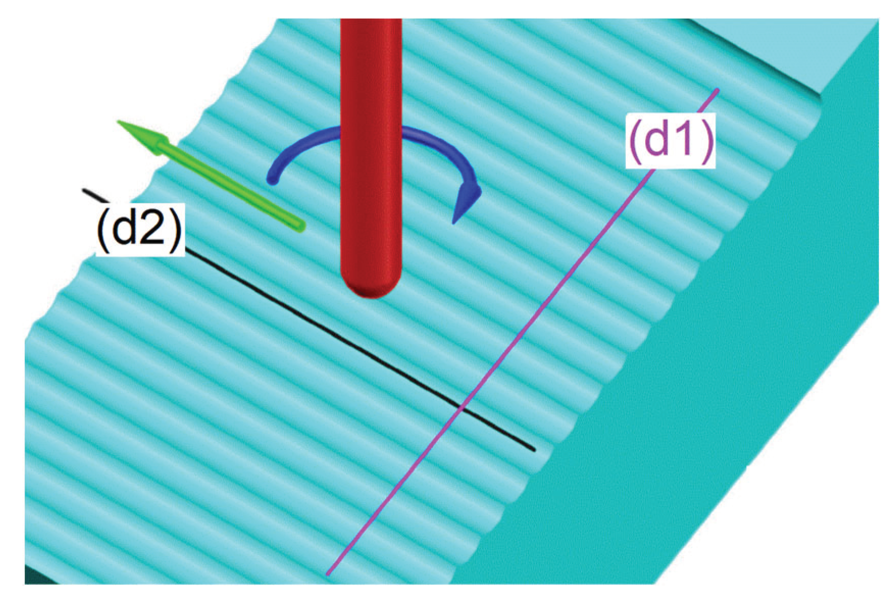
Figure 1 presents a down milling process conceptual description (with the work piece in cyan color, the tool in red, the feed direction in green, the rotation sense in blue). The magenta colored straight line (d1) depicts the pick direction; the black colored line (d2) depicts the feed direction, both used conventionally for experimentally sampling of 2DRP (with a SURFTEST SV-2100W4 contact profilometer, from Mitutoyo).
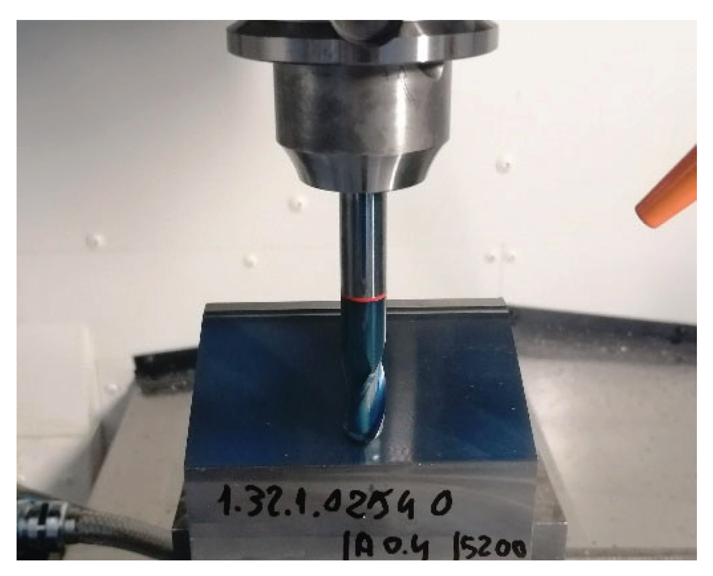
Figure 2 presents a view of tool and work piece (with the cutting process stopped) on a vertical machining center CNC OKUMA GENOS M460R-VE.
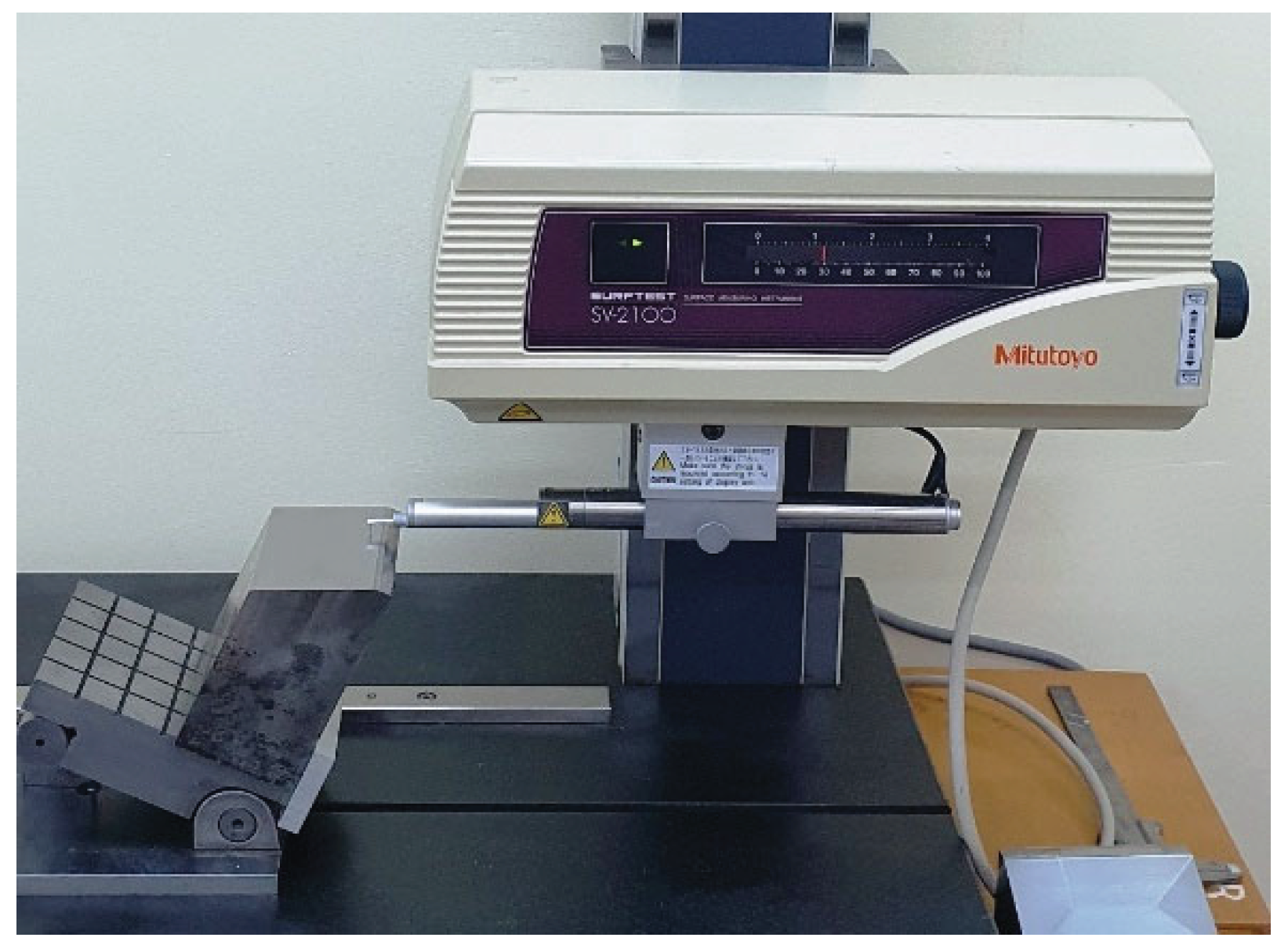
Figure 3 presents a view on the roughness sampling setup, with the flat milled surface placed in horizontal position (here for sampling in pick direction).
The numerical description of a 2DRP is delivered as a two-column .txt files describing 8,000 equidistant samples (
Δx =
0.5 μm sampling interval between samples on
x-axis, for 4 mm total distance). This file is easy loadable in Matlab and analyzable as time-depending signal (by FFT and curve (signal) fitting).
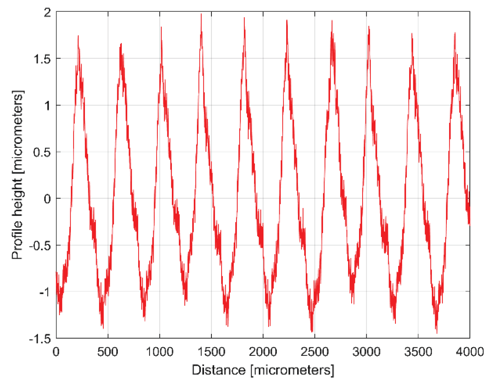
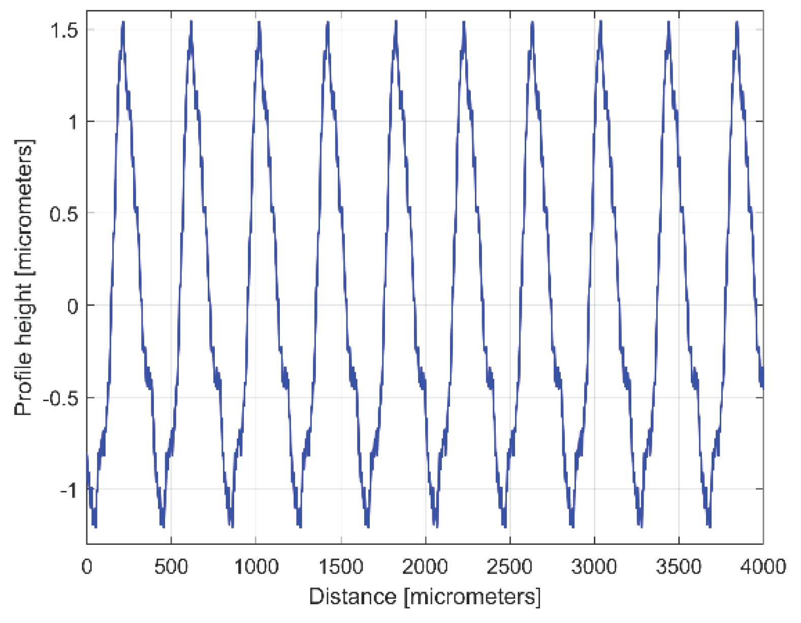
Figure 4 presents a 4 mm length 2DRP, sampled in pick direction (drawn in Matlab). As expected, there is a dominant periodical component inside. A rough estimation on
Figure 4 indicates 10 periods, each period being equal to the milling step over (400 micrometers) and an average pick-interval scallop height of 2.5 micrometers.
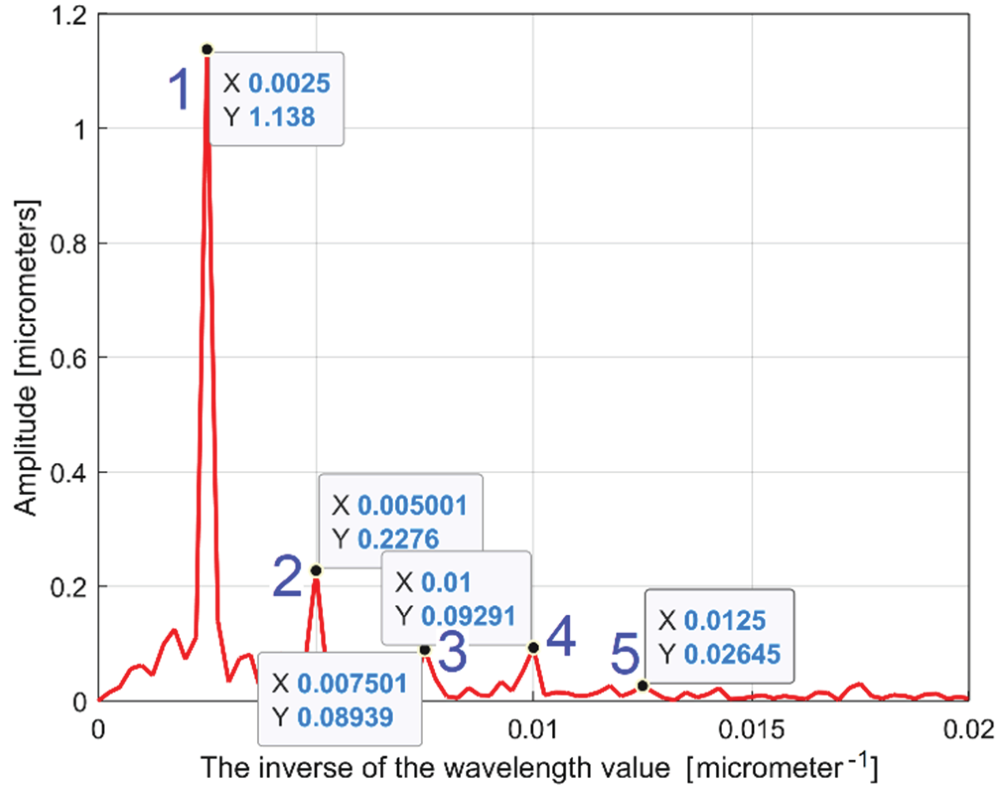
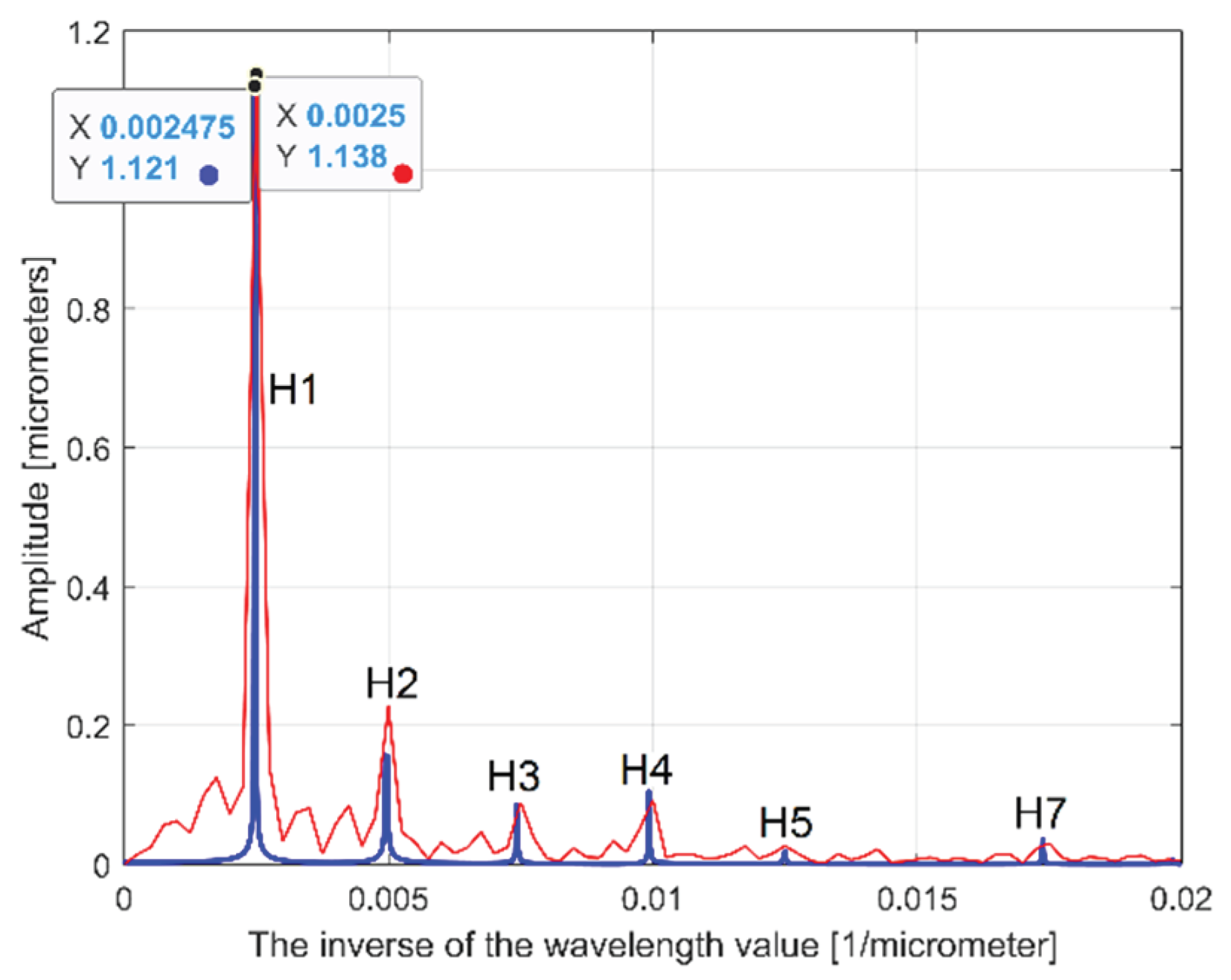
Figure 5 presents a partial view of the FFT spectrum of this 2DRP with real amplitudes (in Matlab). The 2DRP from
Figure 4 was processed in FFT as a time-dependent signal (the
x-coordinates of samples are seen as signal samples time; the
y-coordinates are seen as signal level). The sampling interval
Δx on
x-axis (
Δx=
0.5 μm) is seen as conventional sampling period
Δt on
t-axis. An
x-coordinate on the abscissa of
Figure 5 is the equivalent of a conventional frequency or the inverse of a conventional period or an inverse of a wavelength as well. A peak on FFT spectrum (e. g. the highest peak , depicted by an
x-coordinate of 0.0025 μm
-1 and a
y-coordinate of 1.138 μm) indicates that in the 2DRP exists a dominant sinusoidal component having the wavelength
λ=1/x (e. g.
λ1 = 1/0.0025 = 400 μm for the peak 1). This is exactly the step over value (pick feed) previously highlighted. On
Figure 5 some other relevant peaks (2, 3, 4 and 5) depict sinusoidal components, harmonically correlated with the dominant, the
ith harmonic (with
i =1, 2, 3 and
4) having the wavelengths
λi = λ1/(i+2) as 200, 133.(3), 100 and 80 μm. The conventional sampling period
Δt = 0.5μm depicts the sampling frequency (rate)
fs = 1/ Δt =
2 μm-1 so a conventional Nyquist limit (frequency) of
fNq = fs/
2 = 1μm-1. In other words, the smaller synthetic describable wavelength of a sinusoidal component inside the 2DRP by FFT spectrum is defined as
λmin = (fNq)-1 = (fs/
2)-1 = 1 μm.
However, as it is clear indicated on
Figure 5, the conventional frequency resolution
Rcf = fs/N = 2/8000 = 0.00025 μm-1 is not small enough in order to describe an accurate spectrum. On the spectrum from
Figure 5 there are only
0.02/Rcf = 0.02/0.00025 = 80 samples. There are certainly other higher harmonics that are not visible in spectrum. A longer 2DRP (obtained by increasing the number of samples and keeping the same sampling frequency) reduces significantly the conventional resolution. It must be stated again that the FFT spectrum doesn’t provide the phase at origin of conventional time (
x=0) for sinusoidal components.
A better approach proposed in this paper considers that inside the
y(x) 2DRP is a consistent deterministic part
yd(x) and a less significant non deterministic part
ynd(x), with
y(x) = yd(x) + ynd(x). Generally, for periodical 2DRPs, this deterministic part
yd(x) is describable as a sum of
n sinusoidal components:
In Eq. (1) Aj are amplitudes, 𝜔j are conventional angular frequencies (related by wavelengths λj, with 𝜔j =2π/λj) and φj are conventional phase shifts at origin (x = 0). Here x (the current position of the profilometer stylus on x- axis) plays the role of time.
The curve (signal) fitting procedure (using
Curve fitting tool from Matlab) allows finding out with a good approximation the coefficients
Aj, 𝜔
j and
φj. A sine model (f(x)=a1*sin(b1*x+c1) was used for a first fitting with
x as X data and
y as Y data. In this model a1, b1 and c1 plays the role of
A1, 𝜔
1 and
φ1 coefficients in definition of first sinusoidal component
yd1(x). The first curve fitting produces the results
A1 = 1.151 μm, 𝜔
1 = 0.01558 rad/μm and
φ 1 =
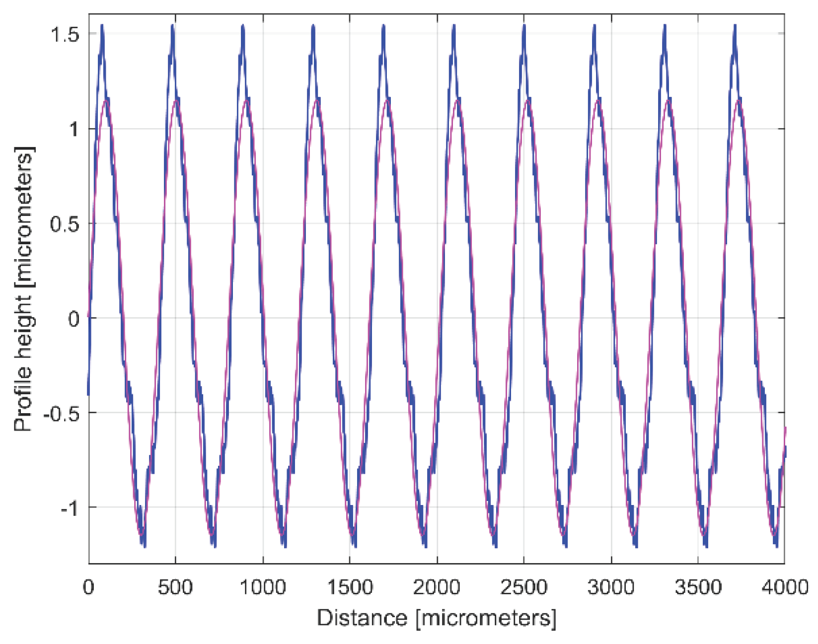
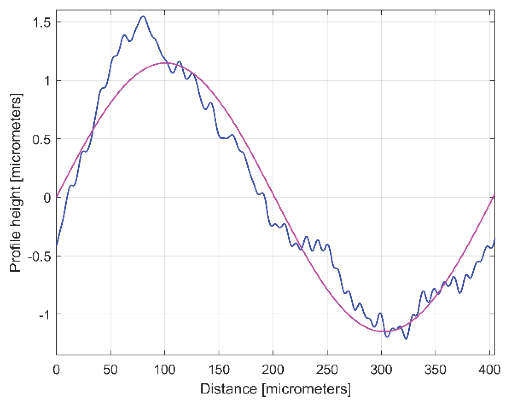
4.1871 rad (usually this fitting procedure find the description of the highest amplitude component). This first sinusoidal component
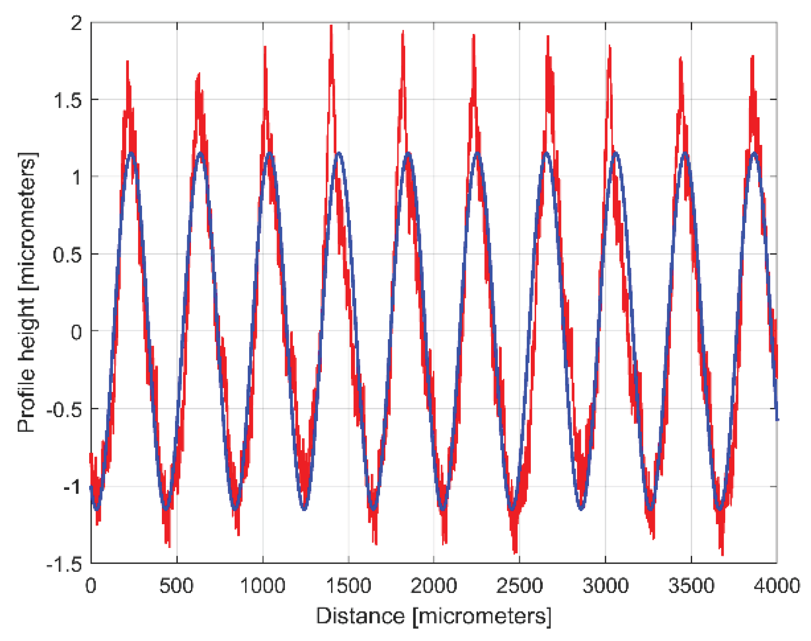
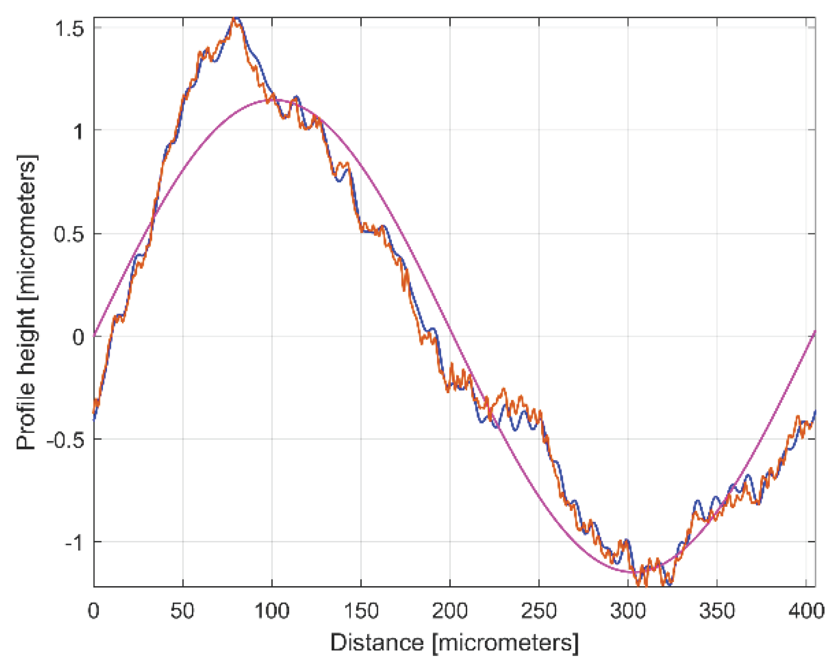
yd1(x) is depicted in blue color on
Figure 6 (as dominant), overlaid on
y(x), depicted in red color (an evolution already described in
Figure 4). Thus the component
yd1(x) can be mathematically described as:
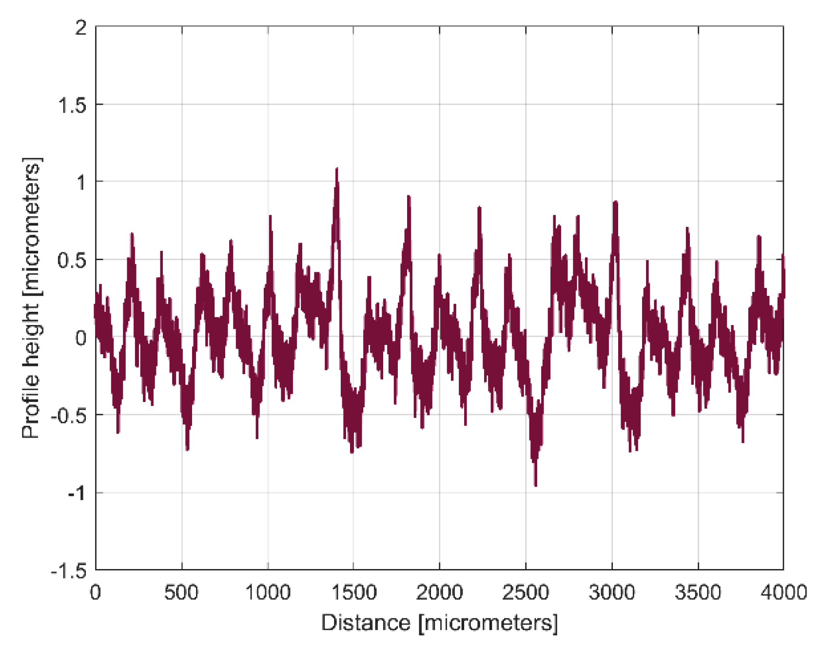
The description of
yd1(x) from Eq. (1) allows the mathematical removing from
y(x), with the result depicted in
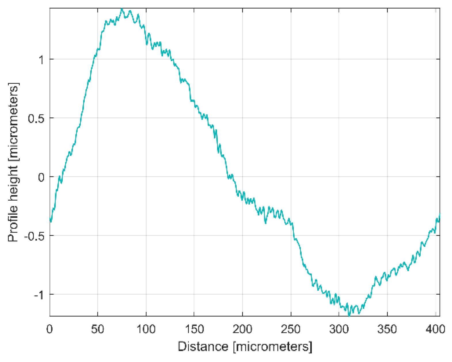
Figure 7, as the first residual (
r1(x)) 2DRP,
r1(x) = y(x)-yd1(x) after first curve fitting (drawn at the same scale with
Figure 6). The decrease of
y-coordinates of the residual profile is a supplementary proof of the quality of
yd1(x) mathematical description.
It is obvious that the dominant component
yd1(x) really fits with
y(x). Its amplitude
A1 is close by this depicted in FFT spectrum (peak 1), its wavelength
λ1 = 2π/𝜔
1 =2π/0.01558 = 403.285 μm, is close by the step over value or pick feed (
400 μm) during the milling process. The conventional frequency of
yd1(x) is
1/λ1 = 0.002479 μm-1, more accurately described by comparison with
Figure 5, related to the first peak (there
1/λ1 = 0.0025 μm). Related by the difference between
λ1 = 403.285 μm (determined by curve fitting) and the pick feed (
400 μm), a logical conclusion must be drawn: we rather suspect the imprecise control of the
x-movement of the contact profilometer during measurement than the pick feed control during milling process.
It is clear that this procedure can be repeated identically (automatically, by programming in Matlab) many times, the mathematical description of the
ydj(x) sinusoidal component can be found by curve fitting of the
(j-1)th residual of 2DRP, as
rj-1(x), described with:
Of course, in curve fitting procedure (as in the case of the FFT spectrum) the exceeding of the Nyquist limit is forbidden (𝜔j <2πfNq or λj > (fNq)-1).
Hypothetically, considering that ynd(x) = 0, a perfect mathematically description of yd(x) (after n curve fitting similar steps), should produce an rn(x) = 0 for the nth residual of 2DRP (graphically representable as a straight line placed on the x-axis).
The viability of this method of determining the mathematical description of a roughness profile (by a similar curve fitting method developed in Matlab) has been demonstrated before [
22] in the analysis of other types of complex signals (vibrations, active electrical power, instantaneous angular speed, etc.) containing many sinusoidal components.
4. Conclusions
The proposed method to analyze and to find (by curve/signal fitting) the mathematical description of the periodical part of an experimental 2D roughness profile, 2DRP (as a sum of sinusoidal components harmonically correlated), provides reliable results, experimentally confirmed, useful to characterize the milled surface (as a sum of wavinesses on two perpendicular directions) and the interaction between the tool and work piece during the milling process (particularly of machined flat surfaces with ball nose end mill, constant step over).
This work proposes an analytical definition of a periodic profile, as a best systematically characterization (pattern) of an experimental 2DRP, sampled with a contact profilometer (in pick and feed directions). A very similar periodic profile (however without an analytical description) is generated using a special kind of sample averaging inside the experimental 2DRP. These periodic profiles are useful for comparison purposes between different experimental 2DRPs or to validate a predictive model for 2DRP [10, 24 and 25] or to achieve the mathematical description of the microgeometry of a milled surface. The shape of these periodic profiles can provide important clues related to the discovery and description of some abnormalities in the milling process (e. g. the tool run out, revealed in this work).
This work proves that the mathematical extrapolation of the analytical defined periodic profile of 2DRP improves the availability of a known but underutilized method of roughness analyzes based on the spectrum of the periodic profile (seen as a time-dependent signal) generated by fast Fourier transform (FFT), with a low (conventional) frequency resolution.
Of course, a generalization of these results in the analysis of other types of milled surfaces (eventually using other roughness sampling methods) is a fully feasible option.
As a future approach, we intend to extend this study to the investigation of the 3D mathematical description of the roughness microgeometry of the complex milled surfaces, experimentally sampled with an appropriate optical system.
Figure 1.
A conceptual description of cutting process.
Figure 1.
A conceptual description of cutting process.
Figure 2.
A view on milling setup.
Figure 2.
A view on milling setup.
Figure 3.
A view on the roughness sampling setup.
Figure 3.
A view on the roughness sampling setup.
Figure 4.
Graphical description of a 2DRP sampled on work piece, in pick direction.
Figure 4.
Graphical description of a 2DRP sampled on work piece, in pick direction.
Figure 5.
A partial view on the FFT spectrum of 2DRP from
Figure 4.
Figure 5.
A partial view on the FFT spectrum of 2DRP from
Figure 4.
Figure 6.
The 2DRP from
Figure 4 (in red) and the first sinusoidal component (
yd1(x)) found by curve (signal) fitting (in blue), Eq. (2).
Figure 6.
The 2DRP from
Figure 4 (in red) and the first sinusoidal component (
yd1(x)) found by curve (signal) fitting (in blue), Eq. (2).
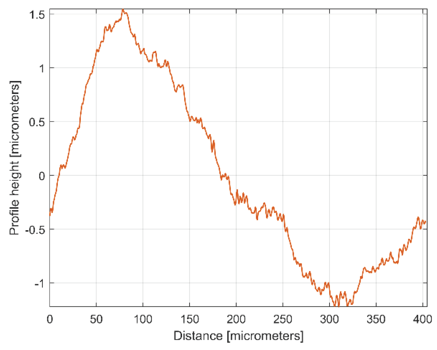
Figure 7.
The first residual 2DRP after first analysis by curve fitting (as r1(x) = y(x)-yd1(x)).
Figure 7.
The first residual 2DRP after first analysis by curve fitting (as r1(x) = y(x)-yd1(x)).
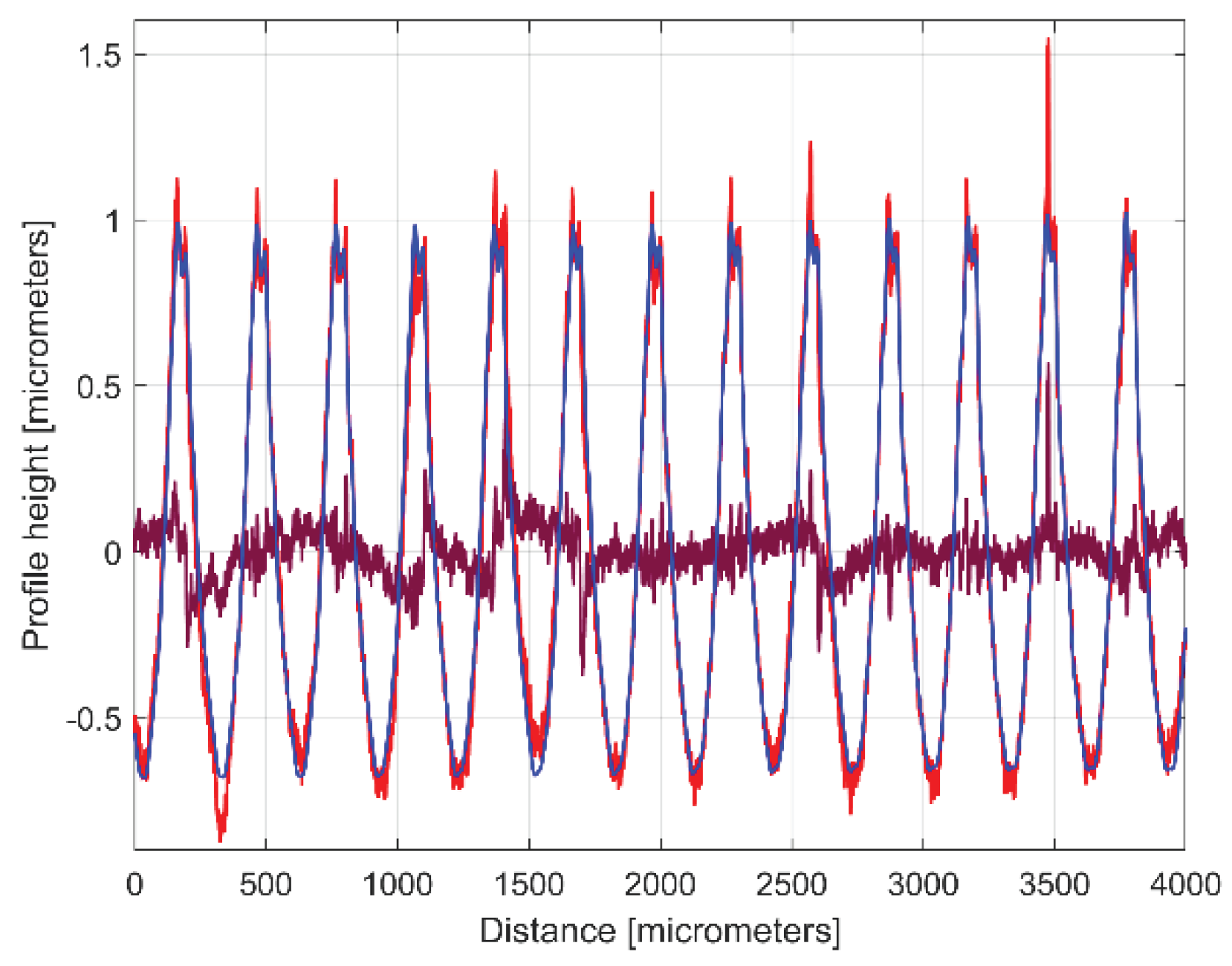
Figure 8.
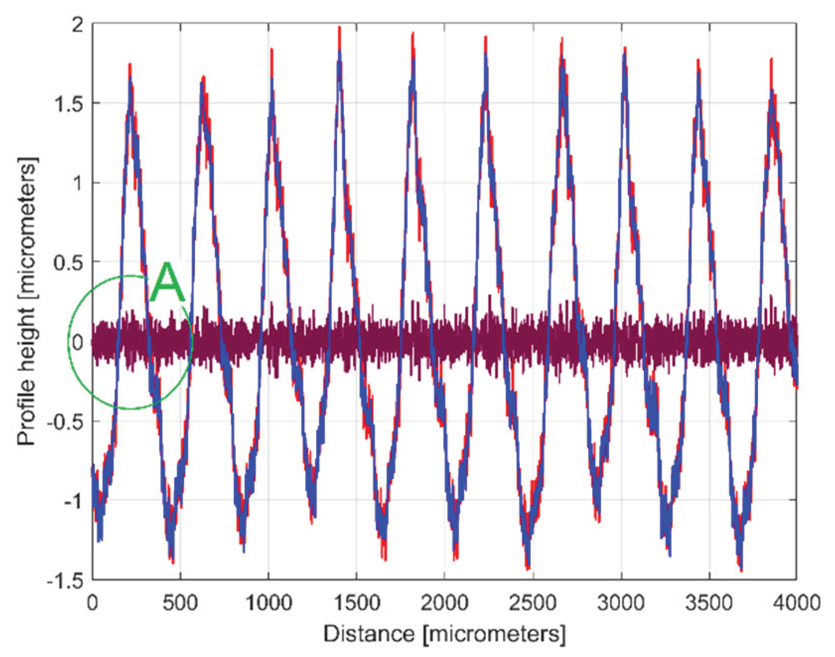
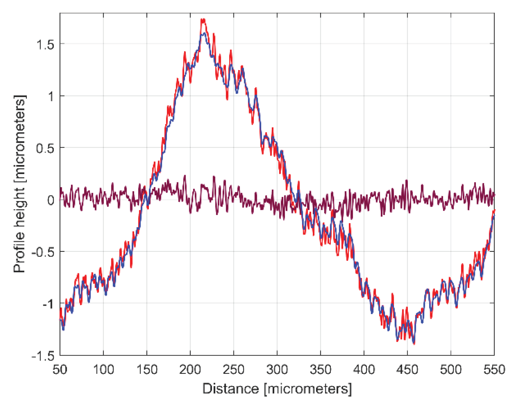
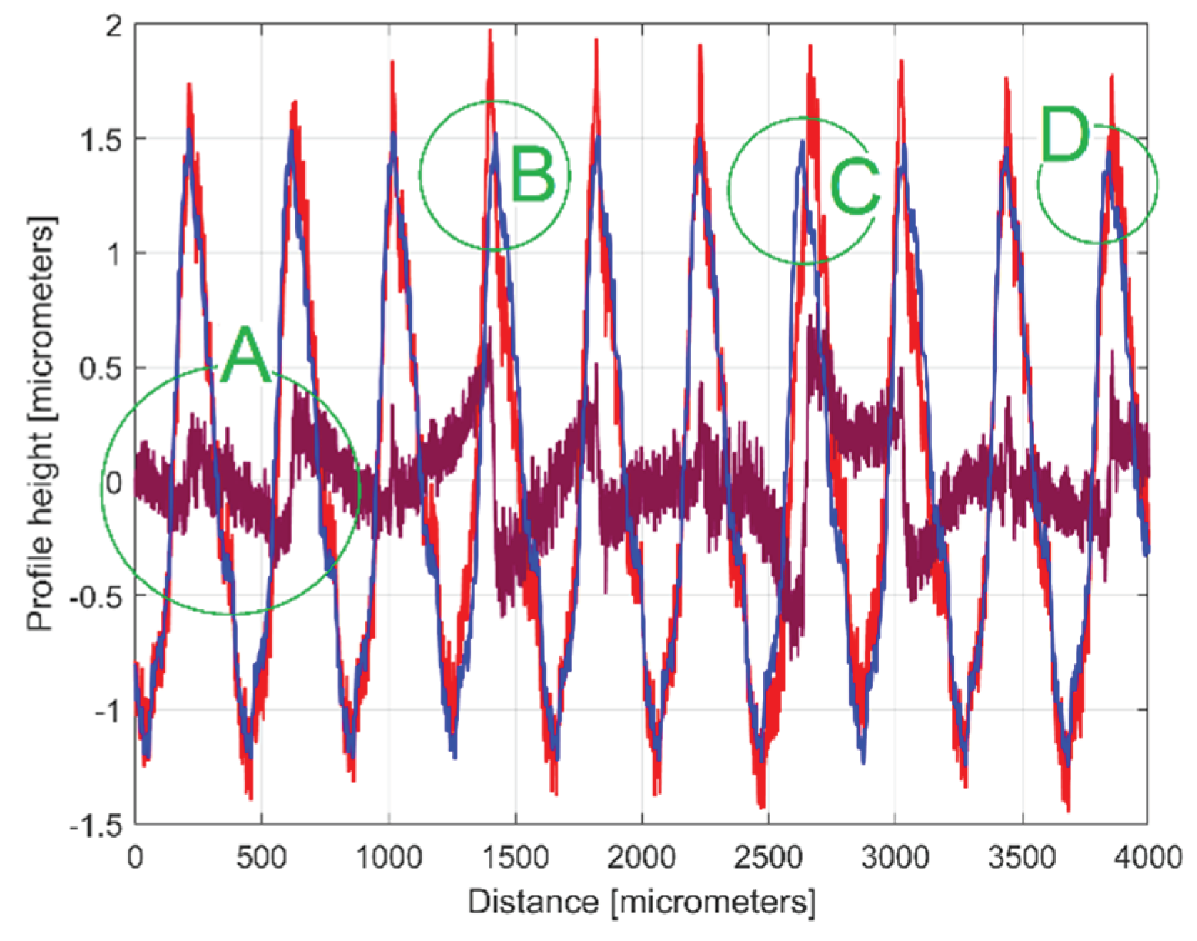
The 2DRP (in red), an approximation of yd(x) with ydh(x) having 122 components (in blue) and the 122th residual r122(x), (in purple).
Figure 8.
The 2DRP (in red), an approximation of yd(x) with ydh(x) having 122 components (in blue) and the 122th residual r122(x), (in purple).
Figure 9.
A zoom-in detail in area A from
Figure 8.
Figure 9.
A zoom-in detail in area A from
Figure 8.
Figure 10.
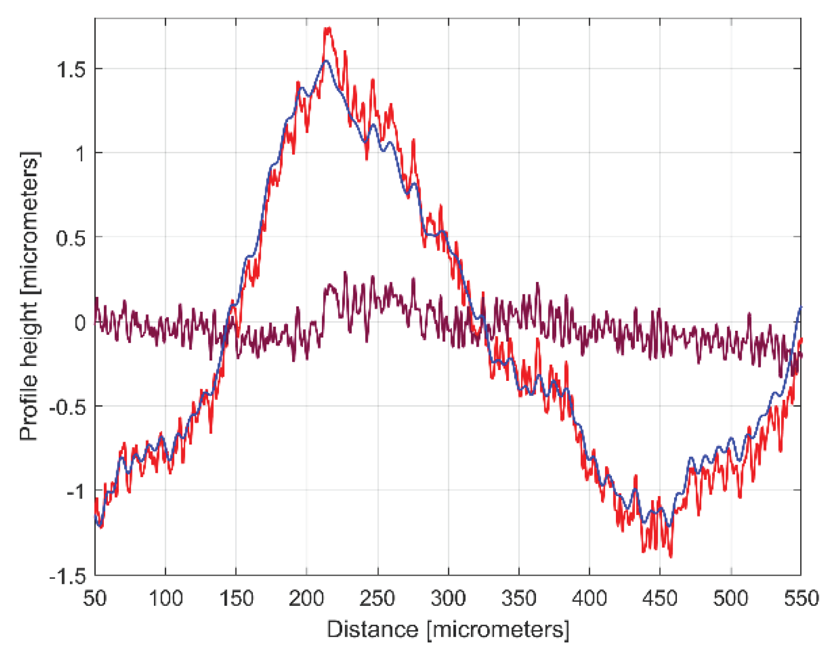
The 2DRP (in red), an approximation of
yd(x) with a
ydh(x) profile having 30 components described in
Table 1 (in blue) and the 30
th residual
r30(x) (in purple).
Figure 10.
The 2DRP (in red), an approximation of
yd(x) with a
ydh(x) profile having 30 components described in
Table 1 (in blue) and the 30
th residual
r30(x) (in purple).
Figure 11.
A zoom-in detail in area A from
Figure 10.
Figure 11.
A zoom-in detail in area A from
Figure 10.
Figure 12.
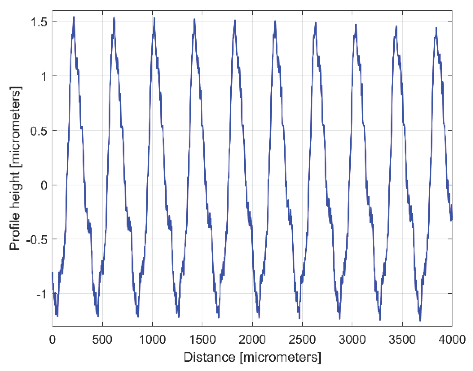
The evolution of ydh(x) profile.
Figure 12.
The evolution of ydh(x) profile.
Figure 13.
The evolution of ydhe(x) profile.
Figure 13.
The evolution of ydhe(x) profile.
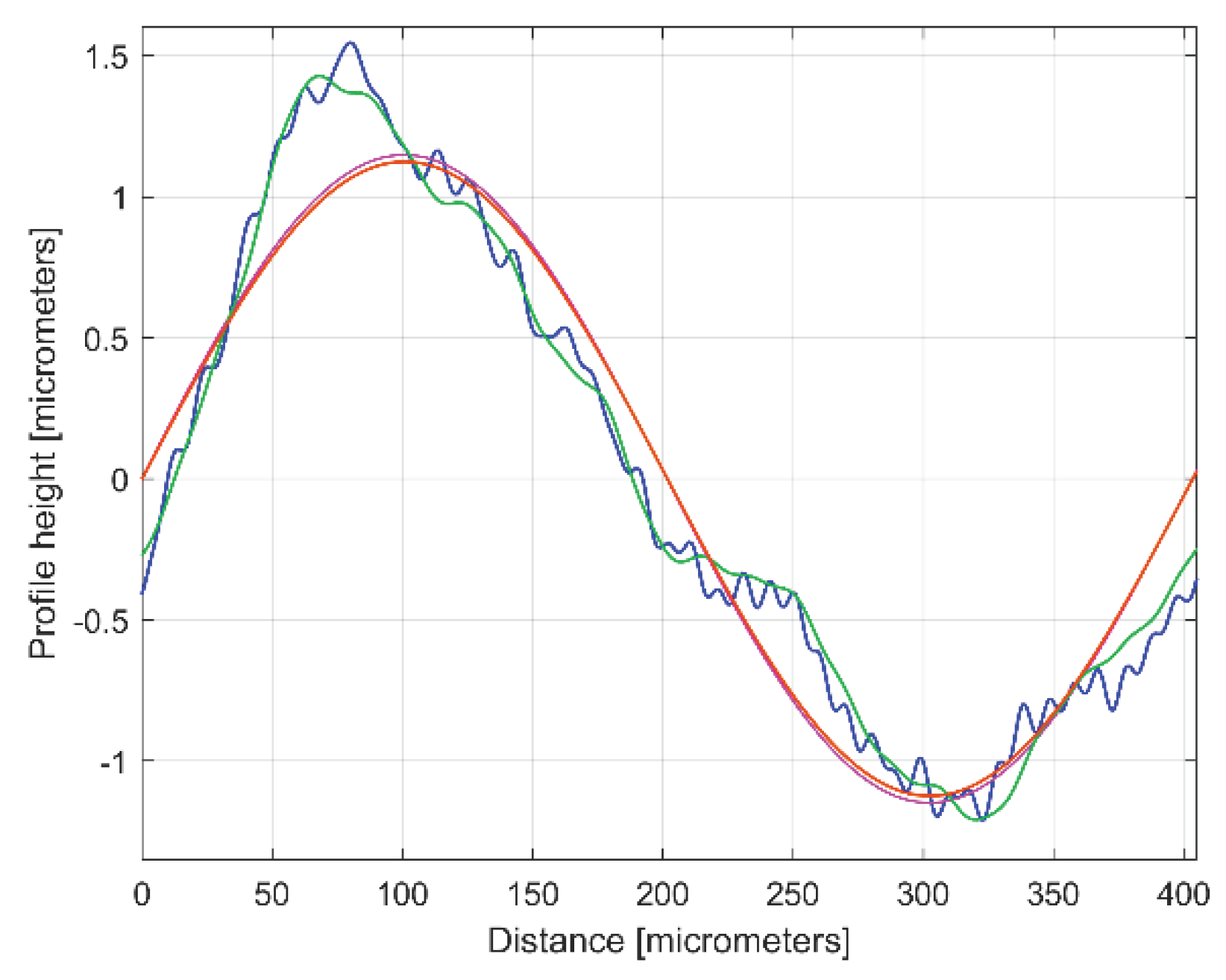
Figure 14.
The evolution of ydhe0(x) profile (in blue) overlaid on the evolution of the dominant component H10 (in magenta).
Figure 14.
The evolution of ydhe0(x) profile (in blue) overlaid on the evolution of the dominant component H10 (in magenta).
Figure 15.
A zoom in detail of
Figure 14 with first period of
ydhe0(x) profile.
Figure 15.
A zoom in detail of
Figure 14 with first period of
ydhe0(x) profile.
Figure 16.
A new 2DRP (in red), an approximation of
yd(x) with
ydh(x) profile having 12 components (in green) and the 12
th residual
r12(x), (in purple). An equivalent of
Figure 10.
Figure 16.
A new 2DRP (in red), an approximation of
yd(x) with
ydh(x) profile having 12 components (in green) and the 12
th residual
r12(x), (in purple). An equivalent of
Figure 10.
Figure 17.
The evolution of
ydhe0(x) profile (in green) overlaid on the evolution of the dominant component H1
0 (in brown). An equivalent of
Figure 14.
Figure 17.
The evolution of
ydhe0(x) profile (in green) overlaid on the evolution of the dominant component H1
0 (in brown). An equivalent of
Figure 14.
Figure 18.
An overlapping of both ydhe0(x) profiles and their dominants H10.
Figure 18.
An overlapping of both ydhe0(x) profiles and their dominants H10.
Figure 19.
A zoom in detail of
Figure 18 with first period of
ydhe0(x) profiles and dominants H1
0.
Figure 19.
A zoom in detail of
Figure 18 with first period of
ydhe0(x) profiles and dominants H1
0.
Figure 20.
The yap0(x) pattern of the first 2DRP.
Figure 20.
The yap0(x) pattern of the first 2DRP.
Figure 21.
The yap0(x) pattern of the first 2DRP, overlaid on the first period of ydhe0(x) profile (in blue) and the dominant, H10.
Figure 21.
The yap0(x) pattern of the first 2DRP, overlaid on the first period of ydhe0(x) profile (in blue) and the dominant, H10.
Figure 22.
The yap0(x) pattern of the 2nd 2DRP.
Figure 22.
The yap0(x) pattern of the 2nd 2DRP.
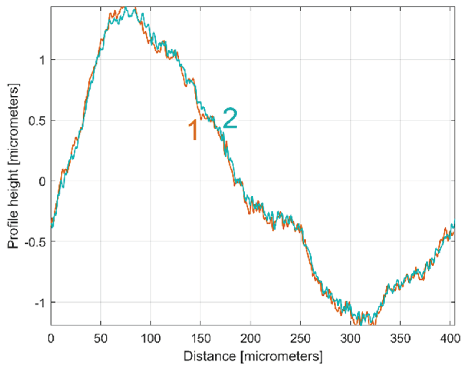
Figure 23.
A graphical overlapping of yap0(x) patterns: 1- for 1st 2DRP; 2 - for 2nd 2DRP.
Figure 23.
A graphical overlapping of yap0(x) patterns: 1- for 1st 2DRP; 2 - for 2nd 2DRP.
Figure 24.
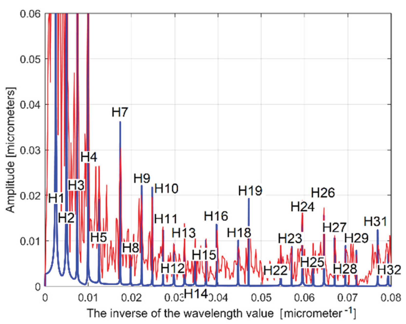
A partial view on the FFT spectra of y(x) profile (in red) and extrapolated ydhe(x) profile with p=10 (in blue).
Figure 24.
A partial view on the FFT spectra of y(x) profile (in red) and extrapolated ydhe(x) profile with p=10 (in blue).
Figure 25.
An extended partial view on the FFT spectra of y(x) profile (in red) and extrapolated ydhe(x) profile with p=10 (in blue).
Figure 25.
An extended partial view on the FFT spectra of y(x) profile (in red) and extrapolated ydhe(x) profile with p=10 (in blue).
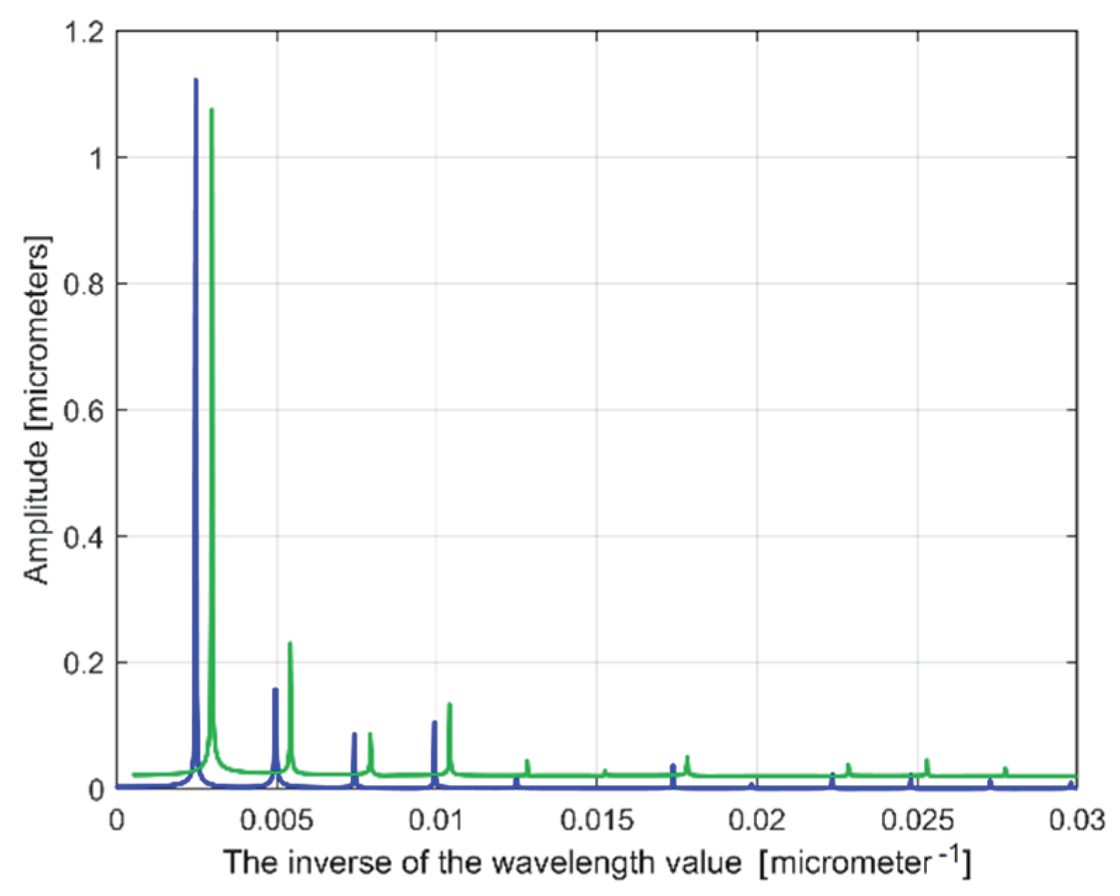
Figure 26.
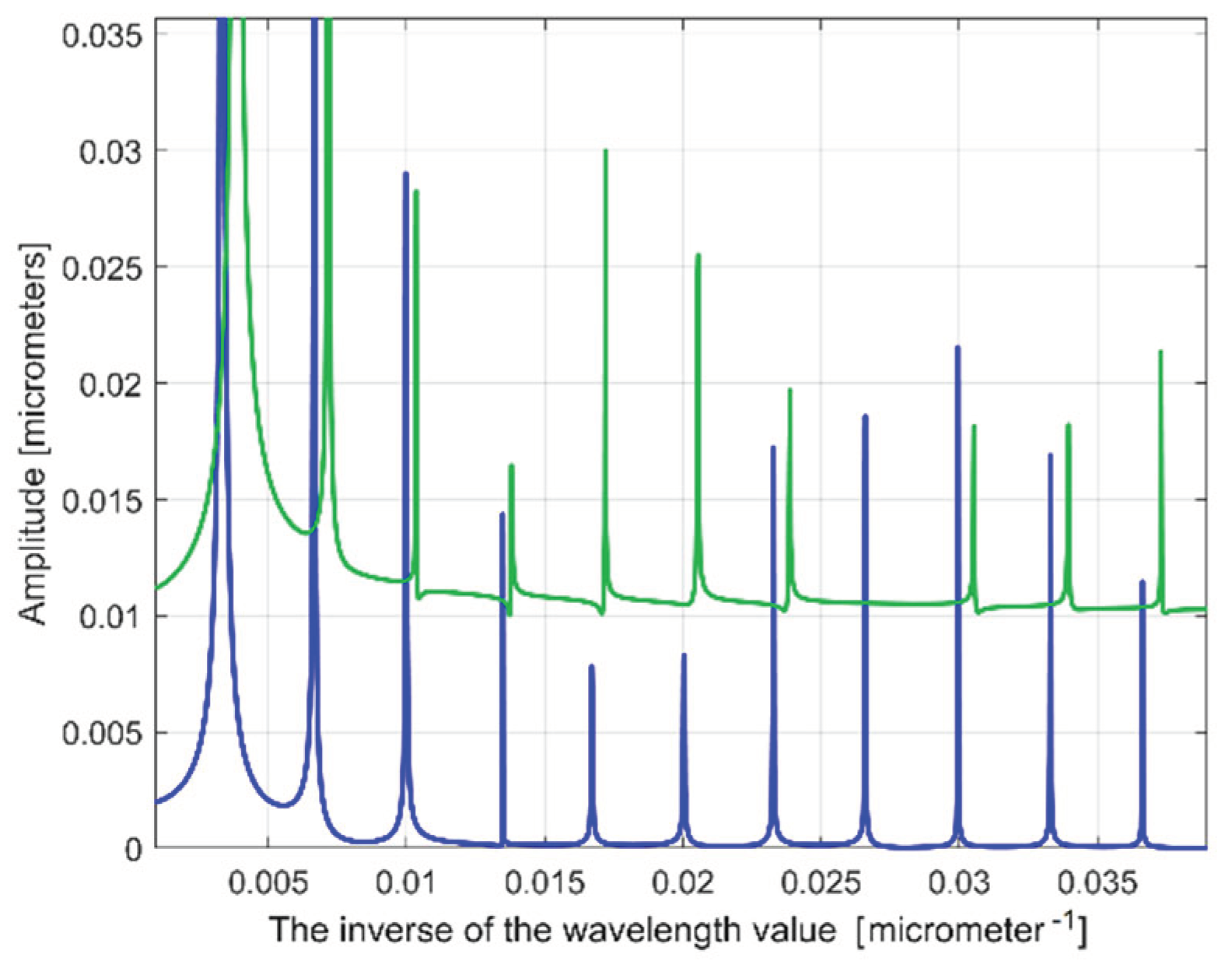
A partial view on the FFT spectra of extrapolated ydhe(x) profiles with p=10 (in blue for 1st 2DRP, in green for 2nd 2DRP).
Figure 26.
A partial view on the FFT spectra of extrapolated ydhe(x) profiles with p=10 (in blue for 1st 2DRP, in green for 2nd 2DRP).
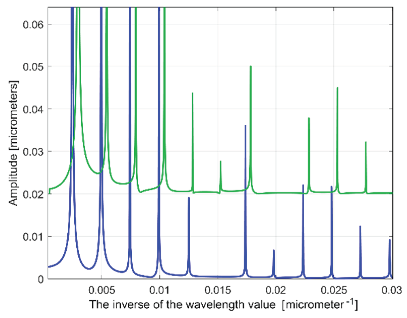
Figure 27.
A zoomed image on
y-axis of the FFT spectra from
Figure 26.
Figure 27.
A zoomed image on
y-axis of the FFT spectra from
Figure 26.
Figure 28.
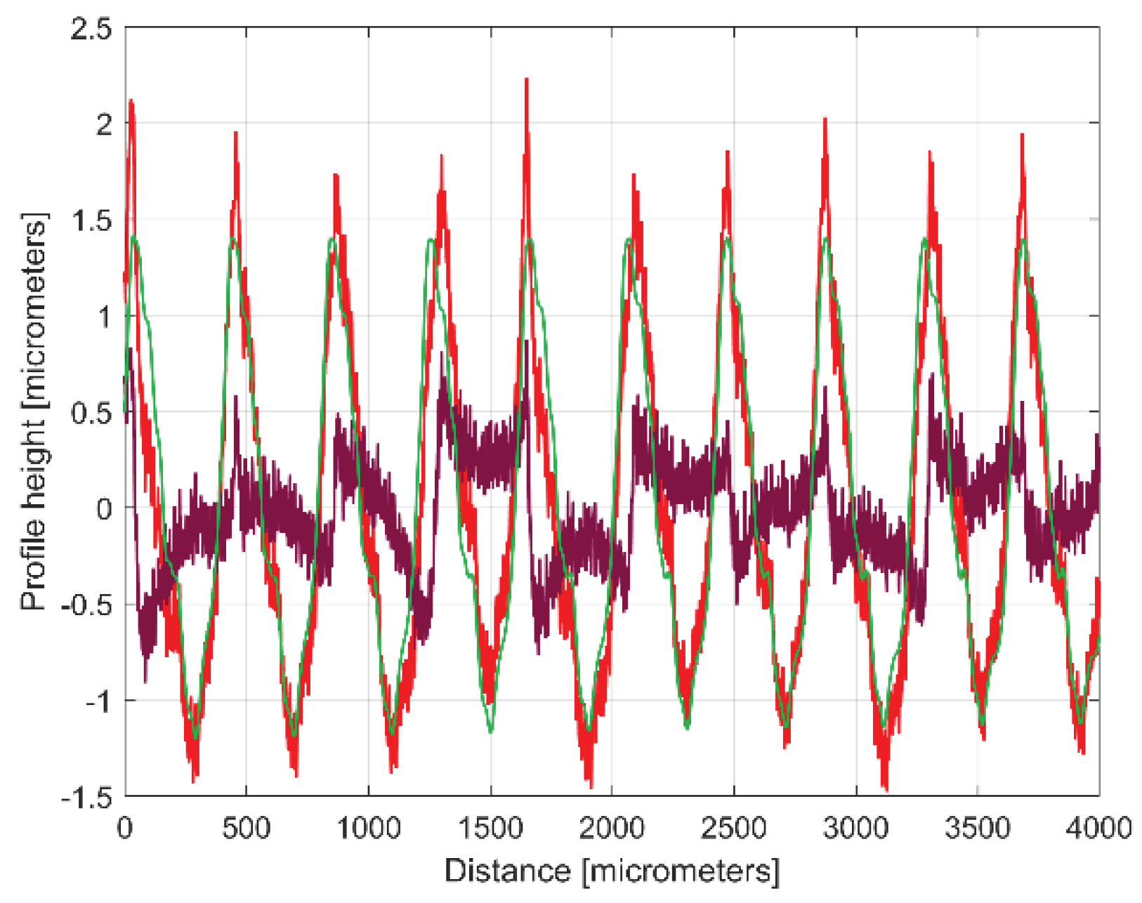
A first 2DRP (in red), the ydh(x) profile (in blue) having 11 components and the 11th residual r11(x) (in purple).
Figure 28.
A first 2DRP (in red), the ydh(x) profile (in blue) having 11 components and the 11th residual r11(x) (in purple).
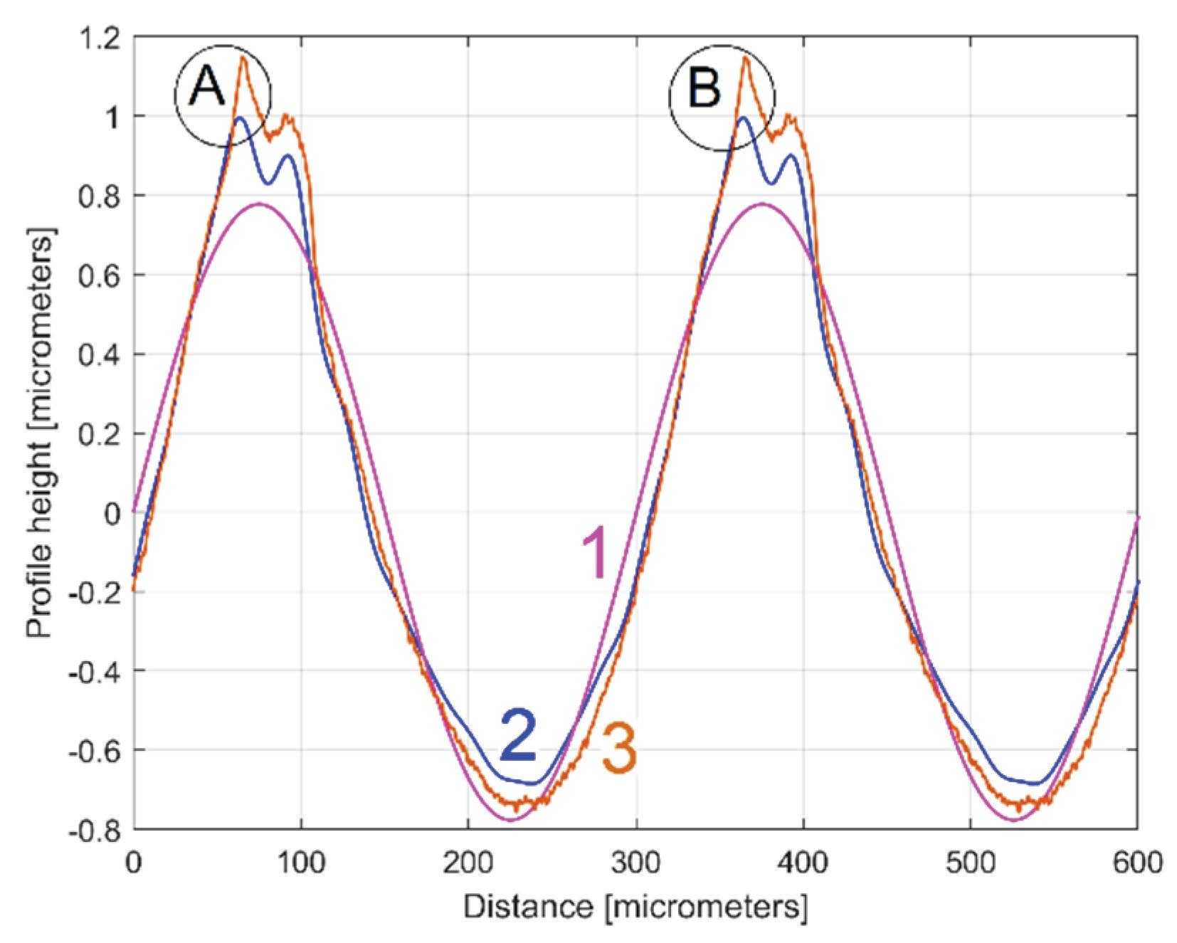
Figure 29.
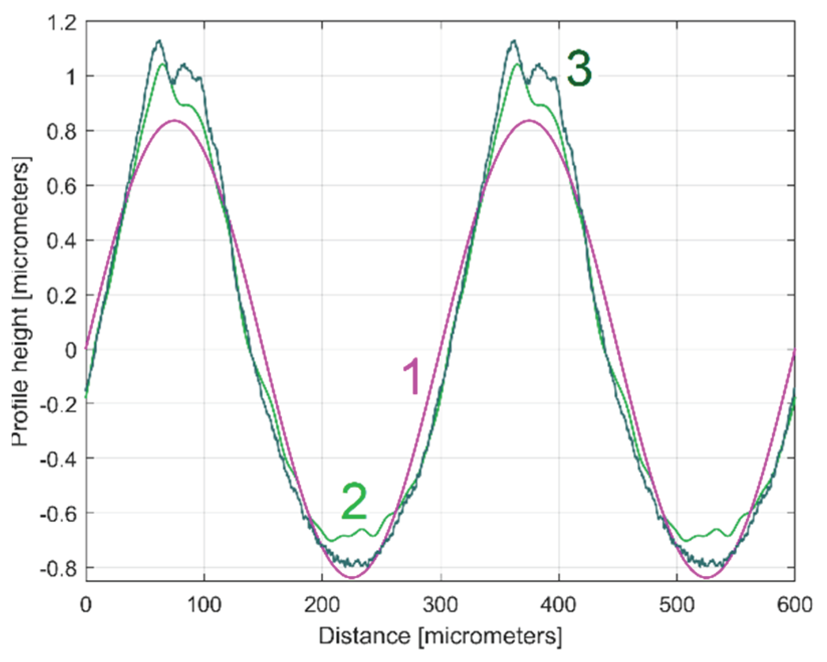
Two conventional periods from: 1 - the dominant component H10; 2 - the profile ydhe0(x); 3 – the pattern yap0(x).
Figure 29.
Two conventional periods from: 1 - the dominant component H10; 2 - the profile ydhe0(x); 3 – the pattern yap0(x).
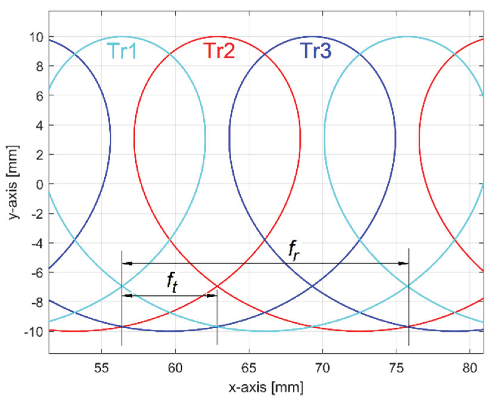
Figure 30.
A simulation of 2D trajectories of points placed on teeth cutting edges (no run out).
Figure 30.
A simulation of 2D trajectories of points placed on teeth cutting edges (no run out).
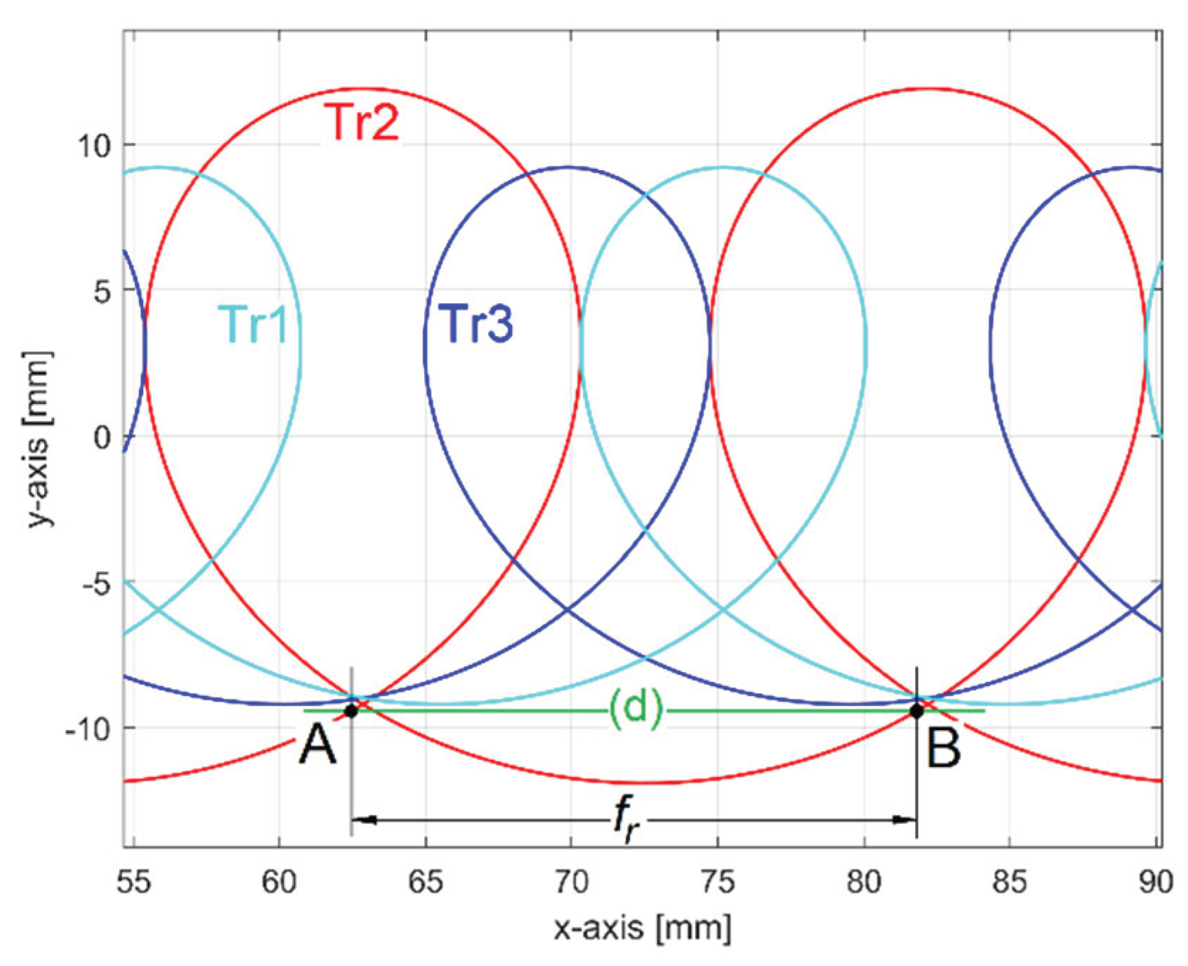
Figure 31.
A simulation of 2D trajectories of points placed on teeth cutting edges (with run out).
Figure 31.
A simulation of 2D trajectories of points placed on teeth cutting edges (with run out).
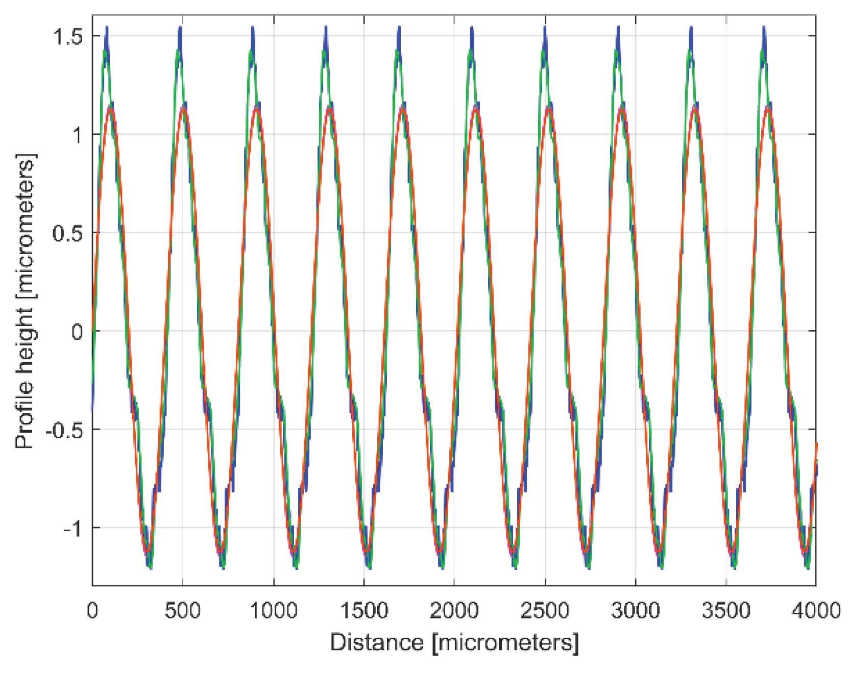
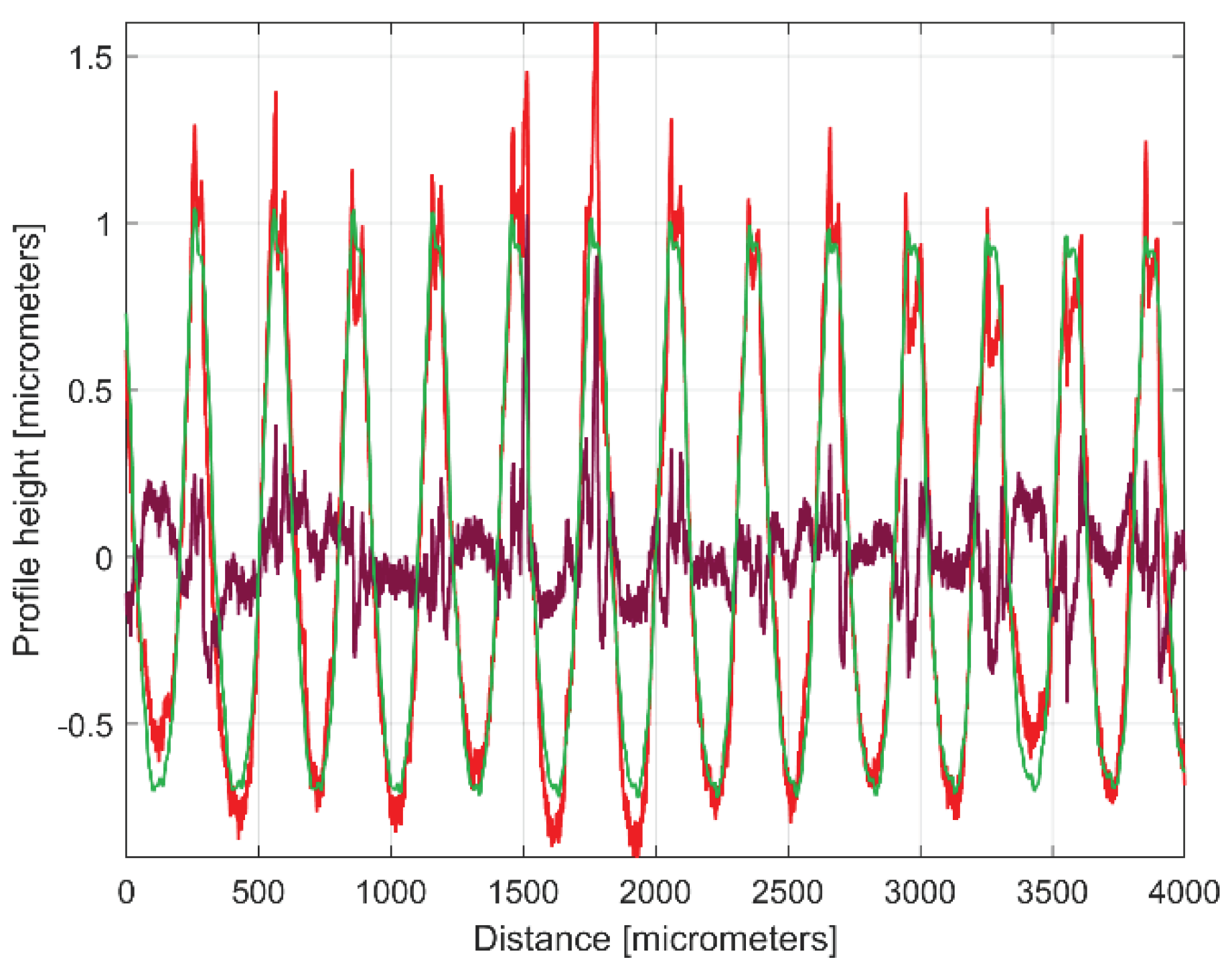
Figure 32.
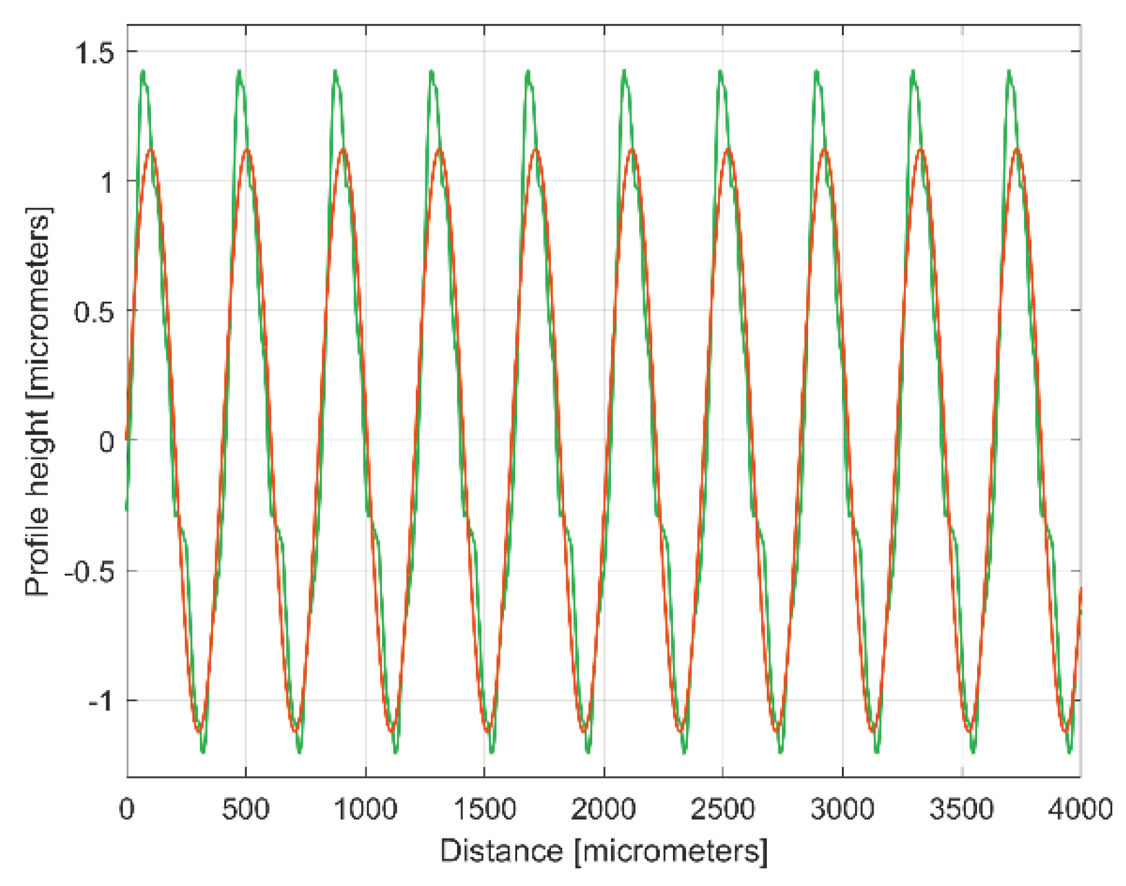
A second 2DRP (in red), the ydh(x) profile (in green) having 11 components and the 11th residual r11(x), (in purple).
Figure 32.
A second 2DRP (in red), the ydh(x) profile (in green) having 11 components and the 11th residual r11(x), (in purple).
Figure 33.
Two conventional periods from: 1 - the dominant component H10; 2 - the profile ydhe0(x); 3 – the pattern yap0(x).
Figure 33.
Two conventional periods from: 1 - the dominant component H10; 2 - the profile ydhe0(x); 3 – the pattern yap0(x).
Figure 34.
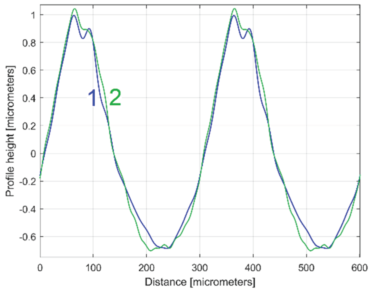
An overlapping of ydhe0(x) profiles for 1st and 2nd 2DRP (1 and 2).
Figure 34.
An overlapping of ydhe0(x) profiles for 1st and 2nd 2DRP (1 and 2).
Figure 35.
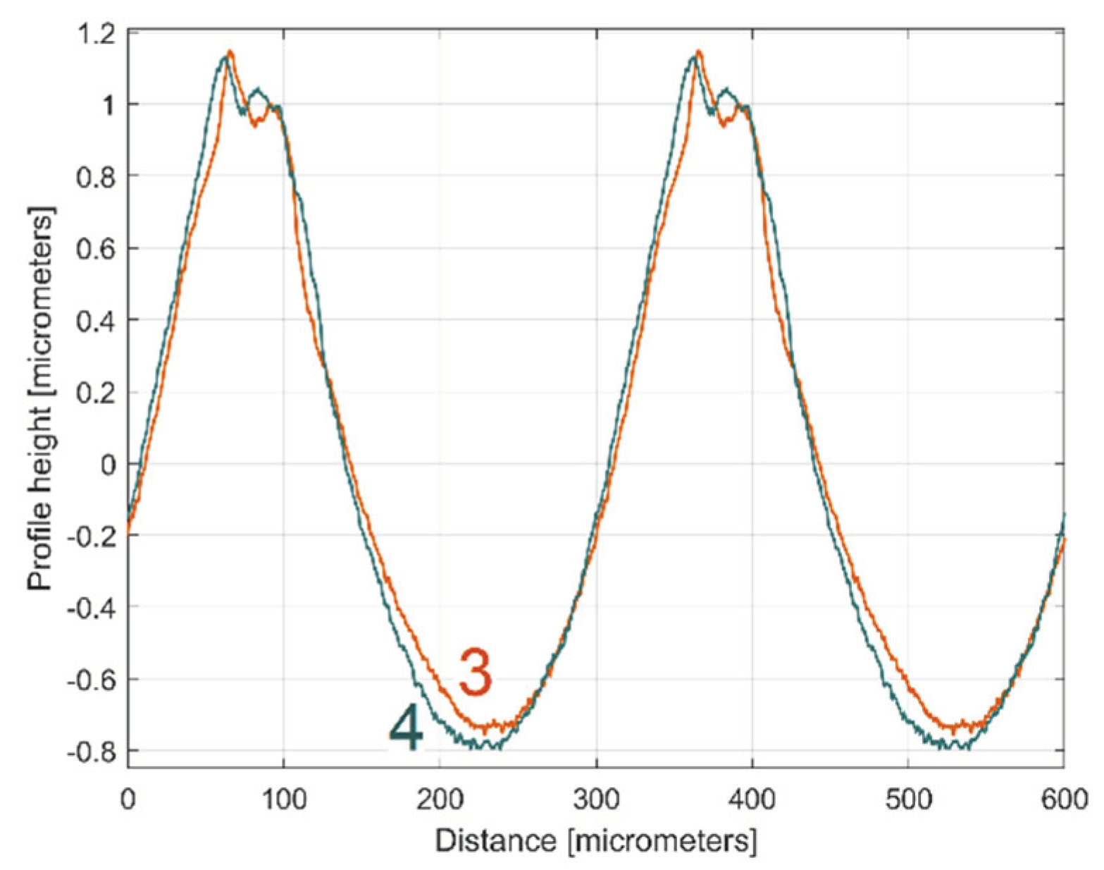
An overlapping of yap0(x) patterns (two periods) for 1st and 2nd 2DRP (3 and 4).
Figure 35.
An overlapping of yap0(x) patterns (two periods) for 1st and 2nd 2DRP (3 and 4).
Figure 36.
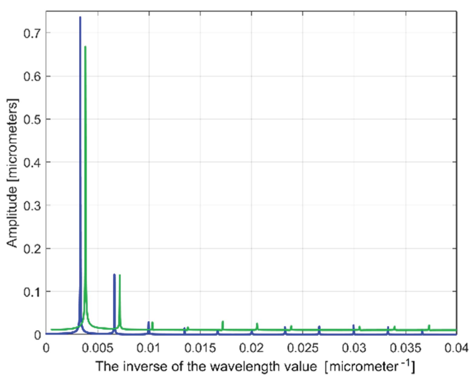
A partial view on the FFT spectra of extrapolated ydhe(x) profiles with p=10 (in blue for first 2DRP, in green for second 2DRP).
Figure 36.
A partial view on the FFT spectra of extrapolated ydhe(x) profiles with p=10 (in blue for first 2DRP, in green for second 2DRP).
Figure 37.
A zoomed image on
y-axis of the FFT spectra from
Figure 36.
Figure 37.
A zoomed image on
y-axis of the FFT spectra from
Figure 36.
Table 1.
The values of constants involved in the mathematical description of 30 well harmonically correlated sinusoidal components inside ydh(x) of the 2DRP, in pick direction.
Table 1.
The values of constants involved in the mathematical description of 30 well harmonically correlated sinusoidal components inside ydh(x) of the 2DRP, in pick direction.
Harmonic #
(Hi) |
Amplitude AHi
[μm] |
Conventional angular frequency 𝜔Hi
[rad/μm] |
Wavelength
λHi =2π/𝜔i
[μm] |
Phase φHi at origin (x=0)
[rad] |
| H1 |
AH1=1.148 |
𝜔H1=0.01557 |
λH1=403.544
|
φH1 =4.2031 |
| H2 |
0.2459 |
0.03118 (as 2.0025· 𝜔H1) |
201.53 (as λH1/2.0024) |
1.412 |
| H3 |
0.09367 |
0.04669 (as 2.9987· 𝜔H1) |
134.57 (as λH1/2.9988) |
4.3261 |
| H4 |
0.1116 |
0.06239 (as 4.0070· 𝜔H1) |
100.70 (as λH1/4.0074) |
2.456 |
| H5 |
0.02461 |
0.07848 (as 5.0404· 𝜔H1) |
80.061 (as λH1/5.0405) |
3.085 |
| H7 |
0.03816 |
0.1092 (as 7.0138· 𝜔H1) |
57.538 (as λH1/7.0135) |
4.785 |
| H8 |
0.009202 |
0.1245 (as 7.9961· 𝜔H1) |
50.467 (as λH1/7.9962) |
5.8120 |
| H9 |
0.0236 |
0.1404 (as 9.0173· 𝜔H1) |
44.752 (as λH1/9.0173) |
3.4731 |
| H10 |
0.02267 |
0.1558 (as 10.0064· 𝜔H1) |
40.328 (as λH1/10.0065) |
4.6591 |
| H11 |
0.0129 |
0.1714 (as 11.0083· 𝜔H1) |
36.658 (as λH1/11.0083) |
1.21 |
| H12 |
0.01171 |
0.1873 (as 12.0295· 𝜔H1) |
33.546 (as λH1/12.0296) |
5.3275 |
| H13 |
0.01317 |
0.2027 (as 13.0186· 𝜔H1) |
30.997 (as λH1/13.0188) |
1.796 |
| H14 |
0.01174 |
0.2181 (as 14.0077· 𝜔H1) |
28.808 (as λH1/14.0081) |
5.8364 |
| H15 |
0.01097 |
0.2337 (as 15.0096· 𝜔H1) |
26.885 as λH1/15.0100) |
5.3481 |
| H16 |
0.01386 |
0.2493 (as 16.0016· 𝜔H1) |
25.203 (as λH1/16.0117) |
3.097 |
| H18 |
0.01152 |
0.2805 (as 18.0154· 𝜔H1) |
22.399 (as λ1/18.0162) |
5.5279 |
| H19 |
0.0192 |
0.2961 (as 19.0173· 𝜔H1) |
21.219 (as λH1/19.0180) |
0.628 |
| H22 |
0.01029 |
0.3425 (as 21.9974· 𝜔H1) |
18.345 (as λH1/21.9975) |
3.9651 |
| H23 |
0.008842 |
0.3586 (as 23.0315· 𝜔H1) |
17.521 (as λH1/23.0320) |
2.8171 |
| H24 |
0.02065 |
0.3741 (as 24.0270· 𝜔H1) |
16.795 (as λH1/24.0276) |
4.3321 |
| H25 |
0.009471 |
0.3896 (as 25.0225· 𝜔H1) |
16.127 (as λH1/25.0229) |
1.299 |
| H26 |
0.01693 |
0.4053 (as 26.0308· 𝜔H1) |
15.502 (as λH1/26.0317) |
1.822 |
| H27 |
0.01081 |
0.4208 (as 27.0263· 𝜔H1) |
14.931 (as λH1/27.0273) |
4.2351 |
| H28 |
0.009238 |
0.4365 (as 28.0347· 𝜔H1) |
14.394 (as λH1/28.0356) |
1.563 |
| H29 |
0.007853 |
0.4524 (as 29.0559· 𝜔H1) |
13.888 (as λH1/29.0570) |
0.7781 |
| H31 |
0.01326 |
0.4833 (as 31.0405· 𝜔H1) |
13.000 (as λH1/31.0418) |
0.5155 |
| H32 |
0.01014 |
0.4985 (as 32.0167· 𝜔H1 |
12.604 (as λH1/32.0171) |
3.9471 |
| H38 |
0.008485 |
0.5924 (as 38.0475· 𝜔H1) |
10.606 (as λH1/38.0487) |
5.7423 |
| H41 |
0.02497 |
0.6392 (as 41.0533· 𝜔H1) |
9.829 (as λH1/41.0565) |
1.478 |
| H42 |
0.01782 |
0.6548 (as 42.0552· 𝜔H1) |
9.595 (as λH1/42.0577) |
0.9996 |
Table 2.
The values of constants involved in the mathematical description of 12 well harmonically correlated sinusoidal components inside ydh(x) of the 2nd 2DRP, sampled in pick direction.
Table 2.
The values of constants involved in the mathematical description of 12 well harmonically correlated sinusoidal components inside ydh(x) of the 2nd 2DRP, sampled in pick direction.
Harmonic #
(Hi) |
Amplitude AHi
[μm] |
Conventional angular frequency 𝜔Hi
[rad/μm] |
Wavelength
λHi =2π/𝜔i
[μm] |
Phase φHi at origin (x=0)
[rad] |
| H1 |
AH1=1.124
|
𝜔H1=0.01552 |
λH1=404.8444
|
φH1 =0.4821
|
| H2 |
0.2406 |
0.03099 (as 1.9968· 𝜔H1) |
202.7488 (as λH1/1.9968) |
0.407 |
| H3 |
0.08159 |
0.04671 (as 3.0097· 𝜔H1) |
134.5148 (as λH1/3.0097) |
5.2621 |
| H4 |
0.1232 |
0.06224 (as 4.0103·𝜔H1) |
100.9509 (as λH1/4.0103) |
6.1897 |
| H5 |
0.0234 |
0.07745 (as 4.9903· 𝜔H1) |
81.1257 (as λH1/4.9903) |
4.9971 |
| H6 |
0.008268 |
0.09263 (as 5.9604· 𝜔H1) |
67.8310 (as λH1/5.9684) |
0.205 |
| H7 |
0.03793 |
0.1088 (as 70103· 𝜔H1) |
57.7499 (as λH1/7.0103) |
3.7771 |
| H9 |
0.01861 |
0.1404 (as 9.0464· 𝜔H1) |
44.7520 (as λH1/9.0464) |
0.1429 |
| H10 |
0.02616 |
0.1558 (as 10.0387· 𝜔H1) |
40.3285 (as λH1/10.0387) |
3.6981 |
| H11 |
0.01256 |
0.1712 (as 11.0309· 𝜔H1) |
36.7008 (as λH1/11.0309) |
2.608 |
| H13 |
0.01106 |
0.2026 (as 13.0541· 𝜔H1) |
31.0128 (as λH1/13.0541) |
2.05 |
| H22 |
0.0107 |
0.3425 (as 22.0683· 𝜔H1) |
18.3451 (as λH1/22.0683) |
1.326 |
