Mathematics of Epidemics: On the General Solution of SIRVD, SIRV, SIRD and SIR Compartment Models

Preprint

Article

Mathematics of Epidemics: On the General Solution of SIRVD, SIRV, SIRD and SIR Compartment Models

Altmetrics

Downloads

172

Views

Comments

A peer-reviewed article of this preprint also exists.

Reinhard Schlickeiser^*

Martin Kröger^*

Reinhard Schlickeiser^*

Martin Kröger^*

This version is not peer-reviewed

Submitted:

14 March 2024

Posted:

15 March 2024

You are already at the latest version

Alerts

Abstract

The susceptible-infected-recovered-vaccinated-deceased (SIRVD) epidemic compartment model extends the SIR model to include the effects of vaccination campaigns and time-dependent fatality rates on epidemic outbreaks. It encompasses the SIR, SIRV, SIRD, and SI models as special cases, with individual time-dependent rates governing transitions between different fractions. We investigate a special class of exact solutions and accurate analytical approximations for the SIRVD and SIRD compartment models. While the SIRVD and SIRD equations pose complex integro-differential equations for the rate of new infections and the fractions as a function of time, a simpler approach considers determining equations for the sum of ratios for given variations. This approach enables us to derive fully exact analytical solutions for the SIRVD and SIRD models. For nonlinear models with a high-dimensional parameter space, such as the SIRVD and SIRD models, analytical solutions, exact or accurately approximative, are of high importance and interest: not only as suitable benchmarks for numerical codes, but especially as they allow us to understand the critical behavior of epidemic outbursts as well as the decisive role of certain parameters. In the second part of our study, we apply a recently developed analytical approximation for the SIR and SIRV models to the more general SIRVD model. This approximation offers accurate analytical expressions for epidemic quantities, such as the rate of new infections and the fraction of infected persons, particularly when the cumulative fraction of infections is small. The distinction between recovered and deceased individuals in the SIRVD model affects the calculation of the death rate, which is proportional to the infected fraction in the SIRVD/SIRD cases but often proportional to the rate of new infections in many SIR models using a posteriori approach. We demonstrate that the temporal dependence of the infected fraction and the rate of new infections differs when considering the effects of vaccinations and when the real-time dependence of fatality and recovery rates diverge. These differences are highlighted for stationary ratios and gradually decreasing fatality rates. \Revised{The case of stationary ratios allows one to construct a new powerful diagnostics method to extract analytically all SIRVD model parameters from measured COVID-19 data of a completed pandemic wave.

Keywords:

Subject: Computer Science and Mathematics - Applied Mathematics

MSC: 34A34; 34A45

1. Introduction

Compartmental mathematical models are very popular and successful to describe the temporal evolution of pandemic and epidemic outbursts in populations of large size (for reviews see ref. [1,2,3]). Their forecasts on hospitalization and death rates help policy makers to install non-pharmaceutical interventions and/or vaccination campaigns at optimized times. As suitable compartments one introduces the fractions of susceptible persons (S), infected persons (I), recovered persons (R), deceased persons (D), and vaccinated persons (V) that no longer can be infected. Individual time-dependent rates regulate the transition between the different compartments. The temporal evolution of the epidemic is then determined by the ratios

k (t) = μ (t) / a (t)

b (t) = v (t) / a (t)

and

q (t) = ψ (t) / a (t)

between the recovery (

μ (t)

), vaccination (

v (t)

) and fatality (

ψ (t)

) rates to the infection (

a (t)

) rate, respectively. By discriminating e.g. between different age classes in each compartment these models can be generalized to a much larger number of compartments in order to investigate the effects of pandemic and epidemic outbursts on persons of certain age groups. However, from the health care point of view to provide sufficiently enough intensive care beds and facilities is independent from the age of the infected persons.

Historically, the first reasonable compartment model was the susceptible–infected–recovered/removed (SIR) epidemic model [4,5,6,7]. This has been refined to include the effect of vaccination campaigns leading to the susceptible–infected–recovered/removed–vaccinated (SIRV) epidemic model [8,9,10,11,12,13,14,15,16,17,18]. The purpose of this manuscript is two-fold. First we will investigate new classes of exact solutions to the SIRVD and SIRD equations. Secondly we will apply the recently developed analytical approximation [19] for the SIR and SIRV models also to the more general SIRVD model. These accurate analytical approximations have been derived for all epidemic quantities of interest such as the rate of new infections

\overset{˚}{J} (t)

and the corresponding cumulative fraction of infections

J (t)

. The main difference between the SIRVD and the SIRV model is the discrimination between recovered and deceased persons by introducing two different compartments. This is necessary as the omicron mutant the COVID-19 has a much smaller (about an order of magnitude) fatality rate than earlier mutants. This gradually changing fatality rate is not accompanied by a corresponding change in the time dependence of the recovery rate. Therefore a mathematical description with one combined recovery/removed compartment is not sufficiently accurate anymore.

The organization of the manuscript is as follows. In Section 2, we introduce the starting dynamical equations for all considered compartment models both in terms of the real time t with respect to the onset of the pandemic, and the reduced time

τ = \int_{0}^{t} d ξ a (ξ)

. It is beneficial for the analysis to express the equations in a form directly involving the observable quantities, such as the cumulative fraction of new infections

J (τ)

and the cumulative fraction of vaccinated persons

V (τ)

. It is shown that for given reduced time variations of the ratios

k (τ)

q (τ)

and

b (τ)

the SIRVD and SIRD equations represent complicated integro-differential equations for the rate of new infections

j (τ)

as well as the cumulative fraction of infections

J (τ)

, or

S (τ)

and

I (τ)

. However, the integro-differential equations can also be regarded as simpler determining equations for the sum of ratios

k (τ) + q (τ) = κ (τ)

for given variations of the ratio

b (τ)

and the fraction

S (τ)

. This new approach is used in Section 3 to derive fully exact analytical solutions for the SIRVD and SIRD models. Especially for the SIRD model it is an effective new method to construct a special class of exact solutions depending on two parameters which are chosen as the values of the ratio

κ (τ)

at the start (

κ (τ = 0)

) and the end (

κ (τ = \infty

) of the epidemic outburst. The new method for the SIRD case is illustrated in Section 4 for three different choices of the two parameters including a detailed investigation of the properties of the constructed solutions.

Section 5 and Section 6 are concerned with the second main purpose of this manuscript, namely the application of the approximate analytical solution in the limit of small cumulative fractions

J ≪ 1

to the SIRVD model. For general reduced time dependencies of the ratios

k (τ)

q (τ)

and

b (τ)

the time dependence of all quantities of interest is derived in Section 5, whereas in Section 6.1 and Section 6.3 two applications are investigated which were inaccessible to analytical treatment before. Of special interest is the calculation of the death rate

d (τ)

and the corresponding cumulative fraction of deceased persons

D (τ)

. Main differences occur between the considered compartment models which reflect two alternative points of view. In Section 6.2 we use the analytic solution and its characteristics to obtain all SIRVD model parameters from reported COVID-19 data.

In the SIRVD and SIRD case with a predescribed fatality rate

ψ (t)

, corresponding to the ratio

q (τ)

, the death rate is proportional to the fraction

I (t)

. Moreover, any different reduced time dependencies of the ratios

k (τ)

and

q (τ)

correctly enter the dynamical equations. In contrast, in the SIR models no compartment of deceased persons has been considered. Instead the total fraction of recovered and removed (by death) populations

R_{tot} (t)

and the summed recovery/removed rate

μ_{tot} (t)

are used. Then the solution for the rate of new infections

{\overset{˚}{J}}_{SIR} (t)

is employed to calculate an a posteriori death rate as [6]

d_{a - pos} = ψ (t) {\overset{˚}{J}}_{SIR} (t)

from a specified fatality rate

ψ (t)

. Of course, this fatality rate can be regarded as part of the summed recovery/removed rate, so that it also enters the dynamical SIR model equations. However, the main difference remains for the calculation of the death rate: in the SIRVD/SIRD cases it is proportional to

I (t)

, whereas in many SIR models it is proportional to

\overset{˚}{J} (t)

. And the temporal dependence of

I (t)

and

\overset{˚}{J} (t)

can be different. As we will show the disparity is most pronounced when the effect of vaccinations is included and/or when the real time dependence of the fatality rate

ψ (t)

and the recovery rate

μ (t)

are different from each other. The a-posteriori approach not necessarily is incorrect but has his own justification. It assumes that the probability to die from the virus infection is only determined by being or having been infected with it, and thus is proportional to the rate of new infections

\overset{˚}{J} (t)

. In contrast in the SIRD and SIRVD models the probability to die is the same on every day being infected and thus depends on the duration of the infection. A summary and conclusion (Section 7) completes the manuscript.

2. Compartment Models

2.1. SIRVD Model

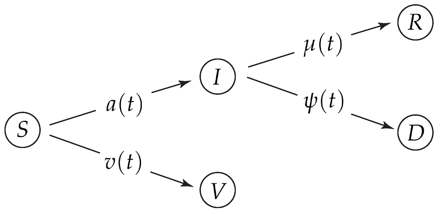
We start with the SIRVD epidemics model described by four transition rates regulating the transitions between the five compartments: the fractions of susceptible persons (S), infected persons (I), recovered persons (R), removed by death persons (D), and vaccinated persons (V) that no longer can be infected. The transition rates in general are time-dependent and different from each other. The infection rate

a (t)

regulates the transition from

S \to I

, the vaccination rate

v (t)

the transition

S \to V

, the fatality rate

ψ (t)

the transition

I \to D

, and the recovery rate

μ (t)

the transition

I \to R

, respectively (Figure 1). The SIRVD equations read:

\begin{matrix} \dot{S} & = & - a (t) S I - v (t) S, \end{matrix}

(1a)

\begin{matrix} \dot{I} & = & a (t) S I - μ (t) I - ψ (t) I, \end{matrix}

(1b)

\begin{matrix} \dot{R} & = & μ (t) I, \end{matrix}

(1c)

\begin{matrix} \dot{D} & = & ψ (t) I, \end{matrix}

(1d)

\begin{matrix} \dot{V} & = & v (t) S, \end{matrix}

(1e)

where the dot stands for a derivative with respect to time t. The five fractions obey the sum constraint

S (t) + I (t) + R (t) + D (t) + V (t) = 1

(2)

at all times

t \geq 0

after the start of the wave at time

t = 0

with the initial conditions of the so-called semi-time case

I (0) = η, S (0) = 1 - η, R (0) = 0, D (0) = 0, V (0) = 0,

(3)

where

η

is positive and usually very small,

η ≪ 1

2.2. SIRV, SIRD, SIR and SI Models

The SIRVD model includes as special cases the SIRV, SIRD and SIR epidemics models. For these three simpler models one introduces the total fraction of recovered and removed (by death) populations

R_{tot} (t) = R (t) + D (t),

(4)

and the summed recovery/removed rate

μ_{tot} (t) = μ (t) + ψ (t) .

(5)

By this modification the five individual compartments of the SIRVD models are reduced to four compartments in the SIRV-description and to three compartments in the SIR-description, respectively. Consequently, the SIRVD Equations (1a)–(2) become

\begin{matrix} \dot{S} & = & - a (t) S I - v (t) S, \end{matrix}

(6a)

\begin{matrix} \dot{I} & = & a (t) S I - μ_{tot} (t) I, \end{matrix}

(6b)

\begin{matrix} {\dot{R}}_{tot} & = & μ_{tot} (t) I, \end{matrix}

(6c)

\begin{matrix} \dot{V} & = & v (t) S, \end{matrix}

(6d)

\begin{matrix} S (t) + I (t) & + & R_{tot} (t) + V (t) = 1, \end{matrix}

(6e)

which apart from a slight change in notation (

R_{tot}

and

μ_{tot}

instead of R and

μ

before) agree exactly with the earlier considered Equations (13) - (17) in [19].

The SIRD and SIR models ignore the effect of vaccinations so that

v (t) = V (t) = 0

. The time evolution in the SIRD model is then given by taking the limit

v (t) = V (t) = 0

of the Equations (1)–(2) yielding

\begin{matrix} \dot{S} & = & - a (t) S I, \end{matrix}

(7a)

\begin{matrix} \dot{I} & = & a (t) S I - μ (t) I - ψ (t) I, \end{matrix}

(7b)

\begin{matrix} \dot{R} & = & μ (t) I, \end{matrix}

(7c)

\begin{matrix} \dot{D} & = & ψ (t) I, \end{matrix}

(7d)

\begin{matrix} S (t) + I (t) & + & R (t) + D (t) + V (t) = 1 . \end{matrix}

(7e)

Likewise, the limit

v (t) = V (t) = 0

of the Equations (6) provide the SIR equations for the three remaining compartments:

\begin{matrix} \dot{S} & = & - a (t) S I - v (t) S, \end{matrix}

(8a)

\begin{matrix} \dot{I} & = & a (t) S I - μ_{tot} (t) I, \end{matrix}

(8b)

\begin{matrix} {\dot{R}}_{tot} & = & μ_{tot} (t) I, \end{matrix}

(8c)

\begin{matrix} S (t) + I (t) & + & R_{tot} (t) = 1 \end{matrix}

(8d)

For completeness we discuss the SI model where additionally

μ (t) = 0

in Appendix A.

2.3. SIRVD Equations in Terms of the Reduced Time Variable

It is convenient to introduce the reduced time [6]

τ = \int_{0}^{t} d ξ a (ξ),

(9)

and the dimensionless ratios

k (τ) = \frac{μ (τ (t))}{a (τ (t))}, b (τ) = \frac{v (τ (t))}{a (τ (t))}, q (τ) = \frac{ψ (τ (t))}{a (τ (t))} .

(10)

Then the SIRVD Equations (1a)–(2) can be written as

\begin{matrix} \frac{d S}{d τ} & = & - S I - b (τ) S, \end{matrix}

(11a)

\begin{matrix} \frac{d I}{d τ} & = & S I - [k (τ) + q (τ)] I, \end{matrix}

(11b)

\begin{matrix} \frac{d R}{d τ} & = & k (τ) I, \end{matrix}

(11c)

\begin{matrix} \frac{d D}{d τ} & = & q (τ) I, \end{matrix}

(11d)

\begin{matrix} \frac{d V}{d τ} & = & b (τ) S, \end{matrix}

(11e)

\begin{matrix} S (τ) + I (τ) & + & R (τ) + D (τ) + V (τ) = 1 . \end{matrix}

(11f)

subject to initial conditions

I (0) = η = 1 - S (0)

and

R (0) = D (0) = V (0) = 0

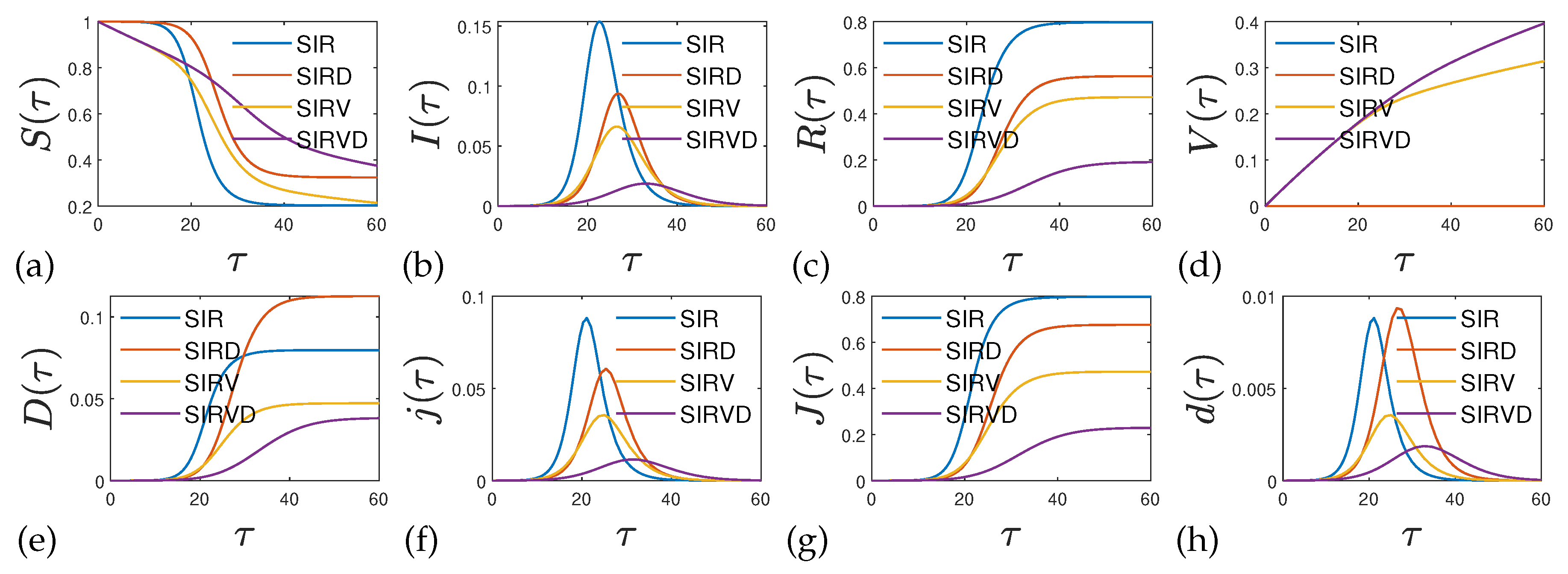
By solving Equations (11) numerically for the case of stationary ratios

k (τ) = 0.5

b (τ) = 0.01

q (τ) = 0.1

, one establishes quantitatively different temporal dependencies for the various fractions of the four different models SIR, SIRD, SIRV and SIRVD (see Figure 2). Numerical schemes have been developed especially for the SIR model, see the recent works [20,21]. We used a variable-step, variable-order (VSVO) Adams-Bashforth-Moulton PECE solver [22] of orders 1 to 13 to produce Figure 2. The highest order used appears to be 12, however, a formula of order 13 is used to form the error estimate and the function does local extrapolation to advance the integration at order 13. This Figure 2 is meant as a motivation for the following analysis which has the aim to understand the different behaviors of the four models on the basis of analytical calculations. Our analytical study also will be concerned with in general time dependent ratios

k (τ)

q (τ)

and

b (τ)

. Moreover, it will derive new methods to construct special classes of exact analytical solutions.

To this end it turns out important to introduce the rate of new infections,

\overset{˚}{J} (t) = a (t) S (t) I (t)

, that determines in the absence of vaccination the reduction of the susceptible compartment according to Equation (1a). Its dimensionless counterpart, appearing in Equation (11a), is

j (τ) = S (τ) I (τ) = \frac{d J (τ)}{d τ},

(12)

so that

\overset{˚}{J} (t) = a (t) j (τ)

and

j (τ = 0) = η (1 - η)

. In terms of the rate of new infections

j (τ)

, and the corresponding cumulative fraction of new infections

J (t) = J (τ) = η + \int_{0}^{τ} d x j (x),

(13)

Equations (11a) and (11e)–(11f) readily provide at all times

J (τ) = 1 - S (τ) - V (τ) = R (τ) + D (τ) + I (τ) .

(14)

Moreover, Equation (11a) yields

\begin{matrix} I (τ) & = & - b (τ) - \frac{d ln S (τ)}{d τ} = - \frac{d V (τ) / d τ}{1 - J (τ) - V (τ)} \\ + \frac{d}{d τ} ln (1 - J (τ) - V (τ)) = \frac{j (τ)}{1 - J (τ) - V (τ)}, \end{matrix}

(15)

where we used Equations (11e), (14) and the first Equation (12). Equation (14) also provides

R (τ) + D (τ) = J (τ) - I (τ) = J (τ) - \frac{j (τ)}{1 - J (τ) - V (τ)} .

(16)

With Equation (15) we obtain for Equations (11c)–(11d)

R (τ) = \int_{0}^{τ} d x k (x) I (x) = \int_{0}^{τ} d x \frac{k (x) j (x)}{1 - J (x) - V (x)},

(17)

and

D (τ) = \int_{0}^{τ} d x q (x) I (x) = \int_{0}^{τ} d x \frac{q (x) j (x)}{1 - J (x) - V (x)},

(18)

implying for the rate of new fatalities

d (τ) = \frac{d D (τ)}{d τ} = q (τ) I (τ) = \frac{q (τ) j (τ)}{1 - J (τ) - V (τ)} .

(19)

2.4. Solution of the SIRVD Equations

With the first Equation (14) one finds

S (τ) = 1 - J (τ) - V (τ),

(20)

so that Equation (11e) can be written in the form

b (τ) = \frac{d V / d τ}{1 - J (τ) - V (τ)},

(21)

yielding

b (τ) [1 - J (τ)] = \frac{d V (τ)}{d τ} + b (τ) V (τ) = e^{- \int_{0}^{τ} d x b (x)} \frac{d}{d τ} [V (τ) e^{\int_{0}^{τ} d x b (x)}] .

(22)

With the initial condition

V (τ = 0) = 0

Equation (22) integrates to

V (τ) = 1 - J (τ) + e^{- \int_{0}^{τ} d x b (x)} [\int_{0}^{τ} d x j (x) e^{\int_{0}^{x} d y b (y)} - (1 - η)],

(23)

providing

S (τ) = 1 - J (τ) - V (τ) = e^{- \int_{0}^{τ} d x b (x)} [1 - η - \int_{0}^{τ} d x j (x) e^{\int_{0}^{x} d y b (y)}] .

(24)

Likewise Equation (11b) can be written as

\begin{matrix} k (τ) + q (τ) & = & S (τ) - \frac{d ln I (τ)}{d τ} = 1 - V (τ) - J (τ) - \frac{d}{d τ} ln [\frac{j (τ)}{1 - V (τ) - J (τ)}], \end{matrix}

(25)

where we used Equations (15) and (24). With the initial conditions Equation (25) integrates to

j (τ) = \frac{d J (τ)}{d τ} = η [1 - V (τ) - J (τ)] exp \int_{0}^{τ} d z (1 - V (z) - J (z) - k (z) - q (z)) .

(26)

A further integration with the initial condition

J (τ = 0) = η

leads to

J (τ) = η [1 + \int_{0}^{τ} d x S (x) e^{\int_{0}^{x} d z [S (z) - k (z) - q (z)]}]

(27)

in terms of

S (τ)

. Furthermore, Equation (25) is equivalent to

\begin{matrix} k (τ) + q (τ) & = & S (τ) - \frac{d}{d τ} [ln j (τ) - ln S (τ)], \end{matrix}

(28)

and also with Equation (11b) integrated to

\begin{matrix} b (τ) & = & - \frac{d ln S (τ)}{d τ} - η exp (\int_{0}^{τ} d z [S (z) - k (z) - q (z)]) . \end{matrix}

(29)

With

S (τ) = (1 - η) exp (- \int_{0}^{τ} d z [I (z) + b (z)])

obtained from Equation (11a), the first Equation (25) is equivalent to

\frac{d ln I (τ)}{d τ} = (1 - η) e^{- \int_{0}^{τ} d z [I (z) + b (z)]} - k (τ) - q (τ) .

(30)

The derived Equations (26)–(30) are nonlinear integro-differential equations for the cumulative fraction of new infections

J (τ)

, and

S (τ)

, respectively. The great advantage of the SIRVD equation written in the form (26) is the direct involvement of observable and monitored quantities, such the cumulative fractions of new infections

J (t) = J (τ)

, and of vaccinated persons

V (t) = V (τ)

. We emphasize that Equations (26)–(29) are exact, and hold for all, the SIR, SIRV, SIRD, and SIRVD models. The only difference is that in the SIRDcase

J_{SIRD} (τ) = 1 - S_{SIRD} (τ)

, because here

b (τ) = V (τ) = 0

, whereas in the SIRVD case

J_{SIRVD} (τ) = 1 - S_{SIRVD} (τ) - V_{SIRVD} (τ)

. If we succeed in either solving the nonlinear integro-differential Equations (26)–(29), or deriving an accurate approximation for their solution, we arrive at a completely analytical solution of all dynamical variables of the SIRVD model and its special cases in dependence on the reduced time

τ

For completeness we note that inserting the exact solution (23) for

V (τ)

in Equation (26) leads to the equivalent nonlinear integro-differential Equations for the rate of new infections

\begin{matrix} j (τ) & = & η [1 - η - \int_{0}^{τ} d x j (x) e^{\int_{0}^{x} d y b (y)}] \times \\ exp \int_{0}^{τ} d z ([1 - η - \int_{0}^{z} d x j (x) e^{\int_{0}^{x} d y b (y)}] e^{- \int_{0}^{z} d y b (y)} - k (z) - q (z) - b (z)) . \end{matrix}

(31)

Before proceeding to the approximation we note that in terms of the real time, the Eqs. (21)–(26) read, with the help of Equations (9), (10), (12), (14), (15), (17), (18), and (31),

\begin{matrix} v (t) & = & \frac{d V / d t}{1 - J (t) - V (t)}, \end{matrix}

(32a)

\begin{matrix} V (t) & = & 1 - J (t) + e^{- \int_{0}^{t} d x v (x)} [\int_{0}^{t} d x \overset{˚}{J} (x) e^{\int_{0}^{x} d y v (y)} - (1 - η)], \end{matrix}

(32b)

\begin{matrix} I (t) & = & \frac{\overset{˚}{J} (t)}{a (t) [1 - J (t) - V (t)]} = \frac{\overset{˚}{J} (t) e^{\int_{0}^{t} d x v (x)}}{a (t) [1 - η - \int_{0}^{t} d x \overset{˚}{J} (x) e^{\int_{0}^{x} d y v (y)}]}, \end{matrix}

(32c)

\begin{matrix} R (t) & = & \int_{0}^{t} d t^{'} \frac{μ (t^{'}) \overset{˚}{J} (t^{'})}{a (t^{'}) [1 - J (t^{'}) - V (t^{'})]} = \int_{0}^{t} d t^{'} \frac{μ (t^{'}) \overset{˚}{J} (t^{'}) e^{\int_{0}^{t^{'}} d x v (x)}}{a (t^{'}) [1 - η - \int_{0}^{t^{'}} d x \overset{˚}{J} (x) e^{\int_{0}^{x} d y v (y)}]}, \end{matrix}

(32d)

\begin{matrix} D (t) & = & \int_{0}^{t} d t^{'} \frac{ψ (t^{'}) \overset{˚}{J} (t^{'})}{a (t^{'}) [1 - J (t^{'}) - V (t^{'})]} = \int_{0}^{t} d t^{'} \frac{ψ (t^{'}) \overset{˚}{J} (t^{'}) e^{\int_{0}^{t^{'}} d x v (x)}}{a (t^{'}) [1 - η - \int_{0}^{t^{'}} d x \overset{˚}{J} (x) e^{\int_{0}^{x} d y v (y)}]}, \end{matrix}

(32e)

\begin{matrix} d (t) & = & \frac{ψ (t) \overset{˚}{J} (t)}{a (t) [1 - J (t) - V (t)]} = \frac{ψ (t) \overset{˚}{J} (t) e^{\int_{0}^{t} d x v (x)}}{a (t) [1 - η - \int_{0}^{t} d x \overset{˚}{J} (x) e^{\int_{0}^{x} d y v (y)}]}, \end{matrix}

(32f)

\begin{matrix} \overset{˚}{J} (t) & = & a (t) [1 - J (t) - V (t)] exp \int_{0}^{t} d x (a (x) [1 - V (x) - J (x)] - μ (x) - ψ (x)) \\ = & a (t) [1 - η - \int_{0}^{t} d x \overset{˚}{J} (x) e^{\int_{0}^{x} d y v (y)}] exp \int_{0}^{t} d t^{'} (a (t^{'}) e^{- \int_{0}^{t^{'}} d y v (y)} [1 - η \\ - \int_{0}^{t^{'}} d x \overset{˚}{J} (x) e^{\int_{0}^{x} d y v (y)}] - μ (t^{'}) - ψ (t^{'}) - v (t^{'})) . \end{matrix}

(32g)

In some aspects for negligible vaccinations the resulting SIRD-model is simpler than the SIRVD-model, e.g. here the simpler relation

J (τ) = 1 - S (τ)

holds. As a consequence the general integro-differential equations (26)–(30) derived before are eased. In Appendix B we explicitly list the corresponding equations for the SIRD model.

In the following sections we will derive a class of special exact solutions (Section 3 and Section 4) and derive approximate analytical solutions of Equations (21) and (25) in the limit of small

J (τ) ≪ 1

(Section 5) following our earlier approach [19]. This approximation then leads to analytical approximations of all fractions of the SIRVD epidemics model as a function of time for given time dependencies of the three ratios (10). We will prove its accuracy of this approach by comparing with the exact numerical solutions of these equations for two illustrative examples (Section 6.1 and Section 6.3) of the reduced time dependence of these ratios. The proposed analytical approximation is self-regulating as the final analytical expression for the cumulative fraction

J_{\infty} = {lim}_{t \to \infty} J (t)

after infinite time allows us to check the validity of the original assumption

J (t) = J (τ) \leq J_{\infty} ≪ 1

Before proceeding we discuss the differences in calculating the fractions of recovered and deceased persons in the different models.

2.5. Fraction of Deceased Persons

The main difference between the considered compartment models occurs for the determination of the fraction of deceased persons

D (τ) = D (t)

and the corresponding death rate

d (τ) = d D (τ) / d τ

and

d (t) = (d D (t) / d t) / a (t)

as a function of the reduced and real time. The disparity is most pronounced if the real time dependence of the fatality rate

ψ (t)

and the recovery rate

μ (t)

are different from each other. In the SIRVD and SIRD cases with a predescribed fatality rate

ψ (t)

, corresponding to the ratio

q (τ)

, the death rate is proportional to

I (t)

as given correctly by Equations (18)–(19) and Equations (32e)–(32f). Moreover, the different reduced time dependences of the ratios

k (τ)

and

q (τ)

correctly enter the dynamical Equations (26)–(29).

However, in the SIR models no compartment of deceased persons is considered. As mentioned before, see Equations (4)–(5), here the total fraction of recovered and removed (by death) populations

R_{tot} (t)

and the summed recovery/removed rate

μ_{tot} (t)

are introduced. With the solution for

{\overset{˚}{J}}_{SIR} (t)

and

J_{SIR} (t)

the rate of new fatalities and the fraction of deceased persons are then calculated a posteriori as [6]

d_{SIR} (t) = α {\overset{˚}{J}}_{SIR} (t), D_{SIR} (t) = α J_{SIR} (t),

(33)

with

α = D_{\infty} / J_{\infty}

. The difference to Equations (32e)–(32f), which involve

I (t) = \overset{˚}{J} (t) / [1 - J (t)]

and not directly

\overset{˚}{J} (t)

, is obvious. Only if the temporal dependence of

I (t)

is not drastically different from the temporal dependence of

\overset{˚}{J} (t)

, the a-posteriori approach is justified. As has been emphasized before [19], for COVID-19 outbursts in many countries the monitored cumulative fraction of infected persons

J (t) ≪ 1

has been much smaller than unity at all times, so that then in the SIR model indeed

I (t) ≃ j (t)

While Equation (33) refers to past work, we will in the following allow for time-dependent fatality rates

ψ (t)

so that the a-posteriori death rate is given by

d_{a - pos} (t) = ψ (t) \overset{˚}{J} (t)

corresponding to

d_{a - pos} (τ) = q (τ) j (τ)

(34)

as a function of reduced time. This way, as opposed to the setting (33), the cumulative

D_{a - pos}

at infinite time must not coincide with

D_{\infty}

. Moreover, in the a-posteriori approach the influence of the later introduced fatality rate

ψ (t)

on the dynamical SIR equations is ignored. This is particularly pronounced if the real time dependence of

ψ (t)

differs from the real time dependence of the recovery rate

μ (t)

. We will elaborate on this below with an illustrative example in Section 6.3.

3. Special Exact Solutions

Equations (28)–(31) are complicated integro-differential equations in the SIRVD and SIRD case, respectively, for given reduced time variations of the ratios

k (τ)

q (τ)

and

b (τ)

. Hovever, they can also be regarded as simpler determining Equations for the ratios

k (τ) + q (τ) = κ (τ)

for given variations of the ratio

b (τ)

and the fraction

S (τ)

. This can be used to derive fully exact analytical solutions for the SIRVD and SIRD models.

We know that

S (τ)

starts from the initial values

S (τ = 0) = 1 - η

and monotonically decreases to its final nonnegative value

S (τ = \infty) \geq 0

after finite or infinite time. We also require, in accord with Equation (12) and the initial conditions specified in Section 2.3, that

j (τ = 0) = η (1 - η) .

(35)

Therefore we adopt the reduced time variation

S (τ) = \frac{1 - η + S_{\infty} tanh \frac{τ_{\max}}{τ_{0}} - (1 - η - S_{\infty}) tanh \frac{τ - τ_{\max}}{τ_{0}}}{1 + tanh \frac{τ_{\max}}{τ_{0}}} .

(36)

parameterized by

S_{\infty}

τ_{\max}

, and

τ_{0}

. While

{lim}_{τ \to \infty} S (τ) = S_{\infty}

is formally correct,

S (τ)

may reach zero after finite time

τ_{fin}

. In that case

{lim}_{τ \to \infty} S (τ) = S (τ_{fin}) = 0

, irrespective of the value of the parameter

S_{\infty}

, that may therefore take positive or negative values in the expression (36). One has1

τ_{fin} = τ_{\max} + τ_{0} {tanh}^{- 1} [\frac{1 - η + S_{\infty} tanh (τ_{\max} / τ_{0})}{1 - η - S_{\infty}}]

(37)

from Equation (36). Only if the argument of the

{tanh}^{- 1}

resides in the interval

[- 1, 1]

, a finite

τ_{fin}

exists. We are going to see that the special choice of

S_{\infty} = 0

has to be treated with care; it will allow us to absorb with Equation (36), along with a particular choice for

τ_{0}

, the analytic solution of the SI model, for which

S (τ)

reaches

S_{\infty}

τ_{fin} = \infty

. Moreover, the initial condition

j (0) = η (1 - η)

will be used to establish a relationship between

S_{\infty}

τ_{\max}

, and

τ_{0}

We adopt without loss of generality positive values of

τ_{0} > 0

. The choice (36) implies

\begin{matrix} \frac{d S (τ)}{d τ} & = & - \frac{1 - η - S_{\infty}}{τ_{0} [1 + tanh \frac{τ_{\max}}{τ_{0}}] {cosh}^{2} \frac{τ - τ_{\max}}{τ_{0}}}, \end{matrix}

(38a)

\begin{matrix} \frac{d ln S (τ)}{d τ} & = & - \frac{1 - η - S_{\infty}}{τ_{0} {cosh}^{2} \frac{τ - τ_{\max}}{τ_{0}} (1 - η + S_{\infty} tanh \frac{τ_{\max}}{τ_{0}} - [1 - η - S_{\infty}] tanh \frac{τ - τ_{\max}}{τ_{0}})}, \end{matrix}

(38b)

\begin{matrix} \frac{d ln \frac{d S (τ)}{d τ}}{d τ} & = & - \frac{2 tanh (\frac{τ - τ_{\max}}{τ_{0}})}{τ_{0}} . \end{matrix}

(38c)

With the first Equation (15) we obtain for the dynamical SIRVD equation (25)

\begin{matrix} k (τ) + q (τ) & = & κ (τ) = S (τ) - \frac{d}{d τ} ln (- [b (τ) + \frac{d ln S (τ)}{d τ}]) . \end{matrix}

(39)

After inserting Equations (36) and (38b) this Equation becomes

\begin{matrix} κ (τ) & = & \frac{1 - η + S_{\infty} tanh \frac{τ_{\max}}{τ_{0}} - (1 - η - S_{\infty}) tanh \frac{τ - τ_{\max}}{τ_{0}}}{1 + tanh \frac{τ_{\max}}{τ_{0}}} - \frac{d}{d τ} ln (- b (τ) \\ + \frac{1 - η - S_{\infty}}{τ_{0} {cosh}^{2} \frac{τ - τ_{\max}}{τ_{0}} (1 - η + S_{\infty} tanh \frac{τ_{\max}}{τ_{0}} - [1 - η - S_{\infty}] tanh \frac{τ - τ_{\max}}{τ_{0}})}) . \end{matrix}

(40)

For given reduced time variations

b (τ)

the combined rate (40) corresponding to the fraction

S (τ)

in Equation (36) can be inferred. In the following we simplify our analysis to the SIRD model.

3.1. SIRD Model

The choice (36) implies for the SIRD model

J (τ) = 1 - S (τ)

J_{\infty} = 1 - S_{\infty}

and

\begin{matrix} j (τ) & = & - \frac{d S (τ)}{d τ} = \frac{1 - η - S_{\infty}}{τ_{0} [1 + tanh \frac{τ_{\max}}{τ_{0}}] {cosh}^{2} \frac{τ - τ_{\max}}{τ_{0}}}, \end{matrix}

(41a)

\begin{matrix} j (τ = 0) & = & \frac{(1 - η - S_{\infty}) (1 - tanh \frac{τ_{\max}}{τ_{0}})}{τ_{0}} . \end{matrix}

(41b)

The rate (41a) is of generalized SI-type (see Equation (A5)) with a width

τ_{0}

different from 2 and a general

τ_{\max}

different from

ln (1 - η) / η

. We thus investigate for which conditions generalized SI-type rates exactly solve the SIRD equations.

The requirement (35) demands

\begin{matrix} S_{\infty} & = & (1 - η) [1 - \frac{η τ_{0}}{1 - tanh \frac{τ_{\max}}{τ_{0}}}], \end{matrix}

(42)

\begin{matrix} J_{\infty} & = & η + \frac{η (1 - η) τ_{0}}{1 - tanh \frac{τ_{\max}}{τ_{0}}} = η + \frac{j (τ = 0) τ_{0}}{1 - tanh \frac{τ_{\max}}{τ_{0}}} . \end{matrix}

(43)

We emphasize that the ansatz (41a) includes the SI model as special case. Inserting the SI-values

S_{\infty} = 0

κ (0) = 0

τ_{0} = 2

and

τ_{\max} = 2 {tanh}^{- 1} (1 - 2 η)

, which follows from Equation (42) for

S_{\infty} = 0

, it is straightforward to show that Equation (41a) correctly reproduces the SI-distribution (A5).

The first Equation (41a) then can be written as (Figure 3)

j (τ) = \frac{η (1 - η) {cosh}^{2} \frac{τ_{\max}}{τ_{0}}}{{cosh}^{2} \frac{τ - τ_{\max}}{τ_{0}}} = j (τ = 0) \frac{{cosh}^{2} \frac{τ_{\max}}{τ_{0}}}{{cosh}^{2} \frac{τ - τ_{\max}}{τ_{0}}} .

(44)

Only for

τ_{\max} ≫ τ_{0}

the maximum rate of new infections at

τ = τ_{\max}

is much larger than the initial value

j (τ = 0)

. In this limit

J_{\infty} ≃ \frac{η (1 - η) τ_{0} e^{\frac{2 τ_{\max}}{τ_{0}}}}{2},

(45)

while Equation (39) for

b (τ) = 0

simplifies to

κ (τ) = S (τ) - \frac{d}{d τ} ln (- \frac{d ln S (τ)}{d τ}) .

(46)

Within the remainder of this subsection, we use the simplifying abbreviations

T = \frac{τ}{τ_{0}}, ρ = \frac{τ_{\max}}{τ_{0}}, Y (τ) = T - ρ

(47)

to derive expressions for

κ (0)

and

κ (\infty)

for the two qualitatively different cases of

S_{\infty} = 0

and

S_{\infty} \neq 0

. With the help of Equation (47) the SIRD equation (36) receives the form

S (τ) = \frac{1 - η + S_{\infty} tanh ρ - (1 - η - S_{\infty}) tanh Y}{1 + tanh ρ},

(48)

or equivalently, upon replacing

S_{\infty}

using Equation (42),

\begin{matrix} S (τ) & = & (1 - η) [1 - η τ_{0} {cosh}^{2} ρ (tanh (T - ρ) + tanh ρ)] \\ = & (1 - η) [1 - \frac{η τ_{0}}{coth T - tanh ρ}] . \end{matrix}

(49)

Similarly, using Equation (38b) in Equation (46),

κ (τ)

becomes

\begin{matrix} κ (τ) & = & \frac{2 tanh (Y)}{τ_{0}} + \frac{1 - η + S_{\infty} tanh ρ - (1 - η - S_{\infty}) tanh (Y)}{1 + tanh ρ} \\ - \frac{1 - η - S_{\infty}}{τ_{0} {cosh}^{2} (Y) (1 - η + S_{\infty} tanh ρ - [1 - η - S_{\infty}] tanh (Y))} . \end{matrix}

(50)

Using

Y (0) = - ρ

, the initial value

κ (0)

can be read off from Equation (50). This yields

\begin{matrix} κ (0) & = & 1 - η - \frac{2 tanh ρ}{τ_{0}} - \frac{(1 - η - S_{\infty}) (1 - tanh ρ)}{(1 - η) τ_{0}} \\ = & 1 - 2 η - \frac{2 tanh ρ}{τ_{0}} = 1 - 2 η - \frac{2 tanh (\frac{τ_{\max}}{τ_{0}})}{τ_{0}}, \end{matrix}

(51)

where we inserted

S_{\infty}

from (42) to arrive at the 2nd line in Equation (51). Expression (51) is valid for any

S_{\infty}

As long as

S_{\infty} \neq 0

, the final value

κ_{\infty} = {lim}_{Y \to \infty} κ (τ)

can be also read off immediately from Equation (50). While the last term in Equation (50) diminishes with increasing Y due to the leading

{cosh}^{2} (Y)

, the first terms readily evaluate upon replacing

tanh (Y)

by unity, so that

\begin{matrix} κ_{\infty} & = & \frac{2}{τ_{0}} + S_{\infty} (S_{\infty} \neq 0) \\ = & \frac{2}{τ_{0}} + (1 - η) [1 - \frac{η τ_{0}}{1 - tanh \frac{τ_{\max}}{τ_{0}}}], \end{matrix}

(52)

where we made use again of

S_{\infty}

from (42). Calculating

κ_{\infty}

for the remaining case of

S_{\infty} = 0

requires more care, as the denominator in the last line of Equation (50) does not anymore increase with increasing Y. For

S_{\infty} = 0

, one instead finds

\begin{matrix} κ_{\infty} & = & \frac{2}{τ_{0}} - \frac{1}{τ_{0}} lim_{Y \to \infty} \frac{1}{{cosh}^{2} (Y) (1 - tanh (Y))} \\ = & \frac{2}{τ_{0}} - \frac{1}{τ_{0}} lim_{Y \to \infty} (1 + tanh Y) = \frac{2}{τ_{0}} - \frac{2}{τ_{0}} = 0 \end{matrix}

(53)

Note the apparent qualitative difference between the two cases. While

κ_{\infty} = S_{\infty}

for

S_{\infty} = 0

, one has

κ_{\infty} = S_{\infty} + 2 / τ_{0}

for

S_{\infty} \neq 0

3.2. Constraints on the Function $κ (τ)$

We recall that values of the function

κ (τ)

smaller than unity describe the epidemic phase where the infection rate

a (t)

is larger than the sum of the recovery and death rate. Hence if still enough susceptible persons are available one expects a rising rate of new infections

\overset{˚}{J} (t)

. In the opposite case of values of the function

κ (τ)

greater than unity the sum of recovery and death rates outnumbers the infection rate so that the rate of new infections will decrease in such a phase. Therefore it is appropriate to start with values of the function

κ (τ)

smaller than unity at small reduced times. Subsequently, the function

κ (τ)

approaches the value

κ_{\infty}

at infinitely large reduced times which can be either smaller or greater than unity depending on the chosen values of

τ_{\max}

and

τ_{0}

. However, not all values for

τ_{0}

and

τ_{\max}

are allowed.

The requirement of having a positive

κ (0) \geq 0

leads to

\frac{1 - 2 η}{2} τ_{0} \geq tanh \frac{τ_{\max}}{τ_{0}}

(54)

This is automatically fulfilled for values of

τ_{0} > \frac{2}{1 - 2 η},

(55)

as the right-hand-side of Equation (55) is always smaller or equal than unity. For values of

τ_{0} \leq 2 / (1 - 2 η)

it is required that

τ_{\max} < τ_{0} {tanh}^{- 1} [\frac{1 - 2 η}{2} τ_{0}] .

(56)

The inequality

S_{\infty} \geq 0

, corresponding to

J_{\infty} \leq 1

, is met as long as the following inequalities hold,

\begin{matrix} tanh \frac{τ_{\max}}{τ_{0}} & \leq & 1 - η τ_{0}, \end{matrix}

(57)

\begin{matrix} τ_{\max} & \leq & τ_{0} {tanh}^{- 1} (1 - η τ_{0}) ≃ \frac{τ_{0}}{2} ln \frac{2}{η τ_{0}} = \sqrt{ln \frac{2}{η τ_{0}}} τ_{0}, \end{matrix}

(58)

that follow from Equation (42). This condition (58), the regime between red and blue dashed lines in Figure 4, is not compatible with condition (56) but holds for certain values of

τ_{0} > 2 / (1 - 2 η)

. The condition (57) further guarantees that also

S (τ)

, and not only

S_{\infty}

, is non-negative at all times because

S \geq 0

requires, according to Equation (49),

tanh ρ + tanh (T - ρ) \leq \frac{1}{η τ_{0} {cosh}^{2} ρ} = \frac{1 - {tanh}^{2} ρ}{η τ_{0}},

(59)

\frac{tanh ρ + tanh (T - ρ)}{1 + tanh ρ} \leq \frac{1 - tanh ρ}{η τ_{0}},

(60)

which is fulfilled for all times

τ

because the left-hand side is always smaller than unity while the right-hand side is larger than unity due to condition (57). In cases

S_{\infty} < 0

, where the condition (57) is not fulfilled,

S (τ_{fin}) = 0

vanishes at the finite time

τ_{fin}

already stated in Equation (37). In this case the chosen solution (36) or (49) can only be used in the finite time interval

0 \leq τ \leq τ_{fin}

Equation (50) can also be written as

\begin{matrix} κ (τ) & = & \frac{2}{τ_{0}} tanh (T - ρ) + (1 - η) [1 - η τ_{0} {cosh}^{2} ρ (tanh (T - ρ) + tanh ρ)] \\ - \frac{η {cosh}^{2} ρ}{{cosh}^{2} (T - ρ) [1 - η τ_{0} {cosh}^{2} ρ (tanh (T - ρ) + tanh ρ)]} \\ = & \frac{2}{τ_{0}} tanh (T - ρ) + (1 - η) [1 - \frac{η τ_{0}}{coth T - tanh ρ}] - \frac{η {cosh}^{2} ρ}{{cosh}^{2} (T - ρ) [1 - \frac{η τ_{0}}{coth T - tanh ρ}]}, \end{matrix}

(61)

where we used the identity

{cosh}^{2} ρ [tanh (T - ρ) + tanh ρ] = \frac{1}{coth T - tanh ρ} .

(62)

The function (61) is positive for

S_{\infty} \geq 0

and non-negative for all times in the admissible interval

0 \leq τ \leq τ_{fin}

. The ratio

κ (τ)

is negative and contains singularities if it is used in the regime

τ > τ_{fin}

4. Details of the Construction of the SIRD Solution

From Equation (51) we obtain, for every

S_{\infty}

tanh (\frac{τ_{\max}}{τ_{0}}) = \frac{1 - 2 η - κ (0)}{2} τ_{0},

(63)

with positive

τ_{0} > 0

. We note that this Equation has a solution provided

1 - 2 η - \frac{2}{τ_{0}} \leq κ (0) \leq 1 - 2 η + \frac{2}{τ_{0}},

(64)

because then the right-hand side of Equation (63) lies within the interval

[- 1, 1]

. While

κ_{\infty} = 0

for

S_{\infty} = 0

, inserting Equation (63) provides for Equation (52),

κ_{\infty} = \frac{2}{τ_{0}} + \frac{(1 - η) [\frac{2}{τ_{0}} + κ (0) - 1]}{\frac{2}{τ_{0}} + κ (0) - 1 + 2 η} (S_{\infty} \neq 0) .

(65)

Setting

y = 2 / τ_{0}

, Equation (65) leads to the quadratic equation

y^{2} + (κ (0) - κ_{\infty} + η) y = κ_{\infty} (κ (0) - 1 + 2 η) - (1 - η) (κ (0) - 1) .

(66)

For general and different values of

κ (0)

und

κ_{\infty}

one can use Equation (66) to determine the implied value of

τ_{0} = 2 / y

and with Equation (63) the resulting value of

τ_{\max}

. The knowledge of

τ_{0}

and

τ_{\max}

then determines for the SIRD model the time variation of the ratio

κ (τ)

for any value of

S_{\infty}

and also of the rate of new infections

j (τ)

in Equation (44). We thus have found an effective new method to construct a special class of exact solutions for the SIRD model which also applies to the SIR model for

ψ (t) = 0

. We illustrate this new method for several cases of the ratios

κ (0)

and

κ_{\infty}

in the next subsections.

4.1. SIRD Solution for $κ_{\infty} = 0$

As discussed there are two cases for which

κ_{\infty} = 0

is realized. If

S_{\infty} = 0

, then

τ_{\inf} = \infty

due to Equation (37), and

tanh (ρ) = 1 - η τ_{0} = \frac{1 - 2 η - κ (0)}{2} τ_{0},

(67)

according to Equations (42) and (63). This Equation (67) determines

τ_{0}

in terms of

κ (0)

, i.e.,

τ_{0} = \frac{2}{1 - κ (0)} . (S_{\infty} = κ_{\infty} = 0)

(68)

With

τ_{0}

at hand,

τ_{\max}

is then also determined by Equation (67). To be specific,

τ_{\max} = \frac{2 {tanh}^{- 1} [1 - (2 η / (1 - κ (0))]}{1 - κ (0)} .

(69)

For the special choice of

κ (0) = κ_{\infty} = S_{\infty} = 0

, one therefore recovers with

τ_{0} = 2

and

τ_{\max} = ln ((1 - η) / η)

the above-mentioned solution of the SI model detailed in Appendix A.

If, on the other hand,

S_{\infty} = - 2 / τ_{0}

is negative, Equation (63), valid for all

S_{\infty}

, yields

τ_{\max} = τ_{0} {tanh}^{- 1} \frac{1 - 2 η - κ (0)}{2} τ_{0},

(70)

so that

τ_{\inf}

from Equation (37) is finite and given by

\begin{matrix} τ_{fin} & = & τ_{\max} + τ_{0} {tanh}^{- 1} (\frac{(η + κ (0)) τ_{0}}{2 + (1 - η) τ_{0}}) \\ = & τ_{0} {tanh}^{- 1} (\frac{1 - 2 η - κ (0)}{2} τ_{0}) + τ_{0} {tanh}^{- 1} (\frac{(η + κ (0)) τ_{0}}{2 + (1 - η) τ_{0}}) . \end{matrix}

(71)

τ_{0}

is also determined by

κ (0)

, as it solves Equation (66) for

κ_{\infty} = 0

, which then simplifies to

y^{2} + (κ (0) + η) y = (1 - η) (1 - κ (0)) .

(72)

The quadratic equation (72) can be solved for

y = 2 / τ_{0}

and thus provides

τ_{0} = \frac{4}{\sqrt{κ^{2} (0) - 2 (2 - 3 η) κ (0) + {(2 - η)}^{2}} - [κ (0) + η]},

(73)

because the 2nd solution leads to negative

τ_{0}

. The

τ_{\max}

is then also determined by

κ (0)

, c.f., Equation (71). For the special choice of

κ (0) = κ_{\infty} = 0

, the above simplifies to

\begin{matrix} τ_{0} & = & \frac{2}{1 - η}, S_{\infty} = - (1 - η), \end{matrix}

(74a)

\begin{matrix} τ_{\max} & = & \frac{2}{1 - η} {tanh}^{1} [1 - \frac{η}{1 - η}] = \frac{ln \frac{2 - 3 η}{η}}{1 - η} ≃ \frac{ln (2 / η)}{1 - η}, \\ τ_{fin} & = & \frac{2}{1 - η} [{tanh}^{- 1} \frac{1 - 2 η}{1 - η} + {tanh}^{- 1} \frac{η}{2 (1 - η)}] \end{matrix}

(74b)

\begin{matrix} = & \frac{1}{1 - η} [ln \frac{2 - 3 η}{η} + ln \frac{2 - η}{η}] ≃ \frac{2 [ln \frac{2}{η} - η]}{1 - η} . \end{matrix}

(74c)

The results of the present section for the extremal case of

κ (0) = 0

are visualized in Figure 5.

We have thus presented the analytic solutions of the SIRD model for the case of

κ_{\infty} = 0

and arbitrary

κ (0)

. There is one solution for which S approaches zero at infinite time, and there is another solution for which S reaches zero at finite time

τ_{fin}

(71). In both cases the characteristic times

τ_{0}

and

τ_{\max}

, as well as

S_{\infty}

appearing in the analytic expression (36) for

S (τ)

are determined by the initial dimensionless rate

κ (0)

and

η = 1 - S (0)

4.2. SIRD Solution for Equal $κ (0) = κ_{\infty} \equiv K \neq 0$

For equal values of

κ (0) = κ_{\infty} \equiv K \neq 0

Equation (66) reduces to

y^{2} + η y = K^{2} - (2 - 3 η) K + (1 - η),

(75)

with the two solutions

y_{1, 2} = - \frac{η}{2} \pm \sqrt{f (K)}, f (K) = K^{2} - (2 - 3 η) K + {(1 - \frac{η}{2})}^{2} .

(76)

The functions

f (K) > 0

is positive for all values of

K > 0

and has the slope

\frac{d f (K)}{d K} = 2 [K - (1 - \frac{3}{2} η)] .

(77)

It therefore decreases for

0 < K \leq K_{0}

with

K_{0} = 1 - (3 η / 2)

, where it attains its minimum

f_{min} = 2 η (1 - η)

. For values

K \geq K_{0}

the function

f (K)

is monotonically increasing. For all values of K one obtains

\sqrt{f (K)} \geq \sqrt{f_{\min}} > (η / 2)

because

η ≪ (8 / 9)

. Hence only the solution

y_{1} (K) = \sqrt{f (K)} - \frac{η}{2} = \sqrt{K^{2} - (2 - 3 η) K + {(1 - \frac{η}{2})}^{2}} - \frac{η}{2}

(78)

is useful as it provides positive values of

τ_{0} (K) = \frac{2}{y_{1} (K)} = \frac{2}{\sqrt{K^{2} - (2 - 3 η) K + {(1 - \frac{η}{2})}^{2}} - \frac{η}{2}} .

(79)

We first check the requirement (64) reading

- y_{1} (K) \leq K - 1 + 2 η \leq y_{1} (K),

(80)

- [\sqrt{f (K)} - \frac{η}{2}] \leq K - 1 + 2 η \leq \sqrt{f (K)} - \frac{η}{2} .

(81)

The left-hand-side of the inequality (81) can be written as

- \sqrt{{(K - K_{0})}^{2} + 2 η (1 - η)} \leq K - K_{0},

(82)

and is fulfilled for all values of

K \geq 0

. This is obvious for

K \geq K_{0}

when the right-hand side of Equation (82) is nonnegative, whereas its left-hand side is negative. For values

0 \leq K < K_{0}

Equation (82) reads

K_{0} - K \leq \sqrt{{(K_{0} - K)}^{2} + 2 η (1 - η)},

(83)

which is fulfilled. Likewise, the right-hand-side of the inequality (81) can be written as

K - (K_{0} - η) \leq \sqrt{{(K - K_{0})}^{2} + 2 η (1 - η)},

(84)

which is fulfilled for values of

K \in (0, K_{0} - η]

, when the left-hand side of Equation (84) is negative while its right-hand side is positive. Recall that the case

K = 0

had been treated in Section 4.1. For large values

K > K_{0} - η

squaring the inequality (84) yields

2 (K - K_{0}) \leq 2 - 3 η = 2 K_{0},

(85)

K \leq 2 K_{0} .

(86)

We conclude that the constraint (81) can be fulfilled for all values of

K \in (0, 2 K_{0}]

. In this interval the solution (79) is given by

τ_{0} (0 < K \leq 2 K_{0}) = \frac{2}{\sqrt{K^{2} - (2 - 3 η) K + {(1 - \frac{η}{2})}^{2}} - \frac{η}{2}} = \frac{2}{\sqrt{{(K - K_{0})}^{2} + 2 η (1 - η)} - \frac{η}{2}},

(87)

and shown in Figure 6. The first derivative of Equation (87) is

\frac{d τ_{0} (K)}{d K} = - \frac{d f / d K}{\sqrt{f (k)} {(\sqrt{f (K)} - \frac{η}{2})}^{2}} = \frac{2 (K_{0} - K)}{\sqrt{f (k)} {(\sqrt{f (K)} - \frac{η}{2})}^{2}},

(88)

so that

τ_{0} (K)

attains its maximum value

τ_{0, E} = \frac{\sqrt{\frac{2}{η}}}{\sqrt{1 - η} - \sqrt{\frac{η}{8}}} = \frac{4}{\sqrt{8 η (1 - η)} - η} = \frac{4}{8 - 9 η} [1 + \sqrt{\frac{8 (1 - η)}{η}}] ≃ \sqrt{\frac{2}{η}},

(89)

K = K_{0}

. Inserting the solution (87) one obtains for Equation (63)

tanh \frac{τ_{\max}}{τ_{0} (K)} = \frac{1 - 2 η - K}{2} τ_{0} (K) = \frac{1 - 2 η - K}{\sqrt{{(K - K_{0})}^{2} + 2 η (1 - η)} - \frac{η}{2}},

(90)

yielding

τ_{\max} (0 < K \leq 2 K_{0}) = \frac{2 {tanh}^{- 1} [\frac{1 - 2 η - K}{\sqrt{{(K - K_{0})}^{2} + 2 η (1 - η)} - \frac{η}{2}}]}{\sqrt{{(K - K_{0})}^{2} + 2 η (1 - η)} - \frac{η}{2}} .

(91)

The solution (91), also shown in Figure 6, is positive for values of

0 < K \leq 1 - 2 η

and negative for values of

1 - 2 η < K \leq 2 K_{0}

due to the property

{tanh}^{- 1} (- x) = - {tanh}^{- 1} (x)

. Obviously

τ_{\max} = 0

for

K = 1 - 2 η

. In order to have positive values of

K_{0}

and the zero

1 - 2 η

we should consider only values of

η < 0.5

For completeness we note an alternative

τ_{\max} (τ_{0})

. Equating the right hand sides of Equations (51) and (52) leads with

R \equiv tanh (ρ) = tanh (τ_{\max} / τ_{0})

1 - 2 η - \frac{2 R}{τ_{0}} = \frac{2}{τ_{0}} + (1 - η) [1 - \frac{η τ_{0}}{1 - R}] .

(92)

Upon multiplying with

(1 - R) τ_{0}

one obtains

(1 - R) [(1 - 2 η) τ_{0} - 2 R] = 2 (1 - R) + (1 - η) (1 - η τ_{0} - R) τ_{0},

(93)

or the quadratic equation

R^{2} + \frac{η τ_{0}}{2} R = 1 + \frac{η τ_{0}}{2} [1 - (1 - η) τ_{0}],

(94)

which is solved by

R = \frac{\pm \sqrt{16 + η τ_{0} [8 - (8 - 9 η) τ_{0}]} - η τ_{0}}{4},

(95)

so that

τ_{\max} = τ_{0} {tanh}^{- 1} [\frac{\pm \sqrt{16 + η τ_{0} [8 - (8 - 9 η) τ_{0}]} - η τ_{0}}{4}] .

(96)

The requirement

| R | \leq 1

is fulfilled for all values of

η < 1

if the argument of the square root in Equation (95) is nonnegative. The last condition leads to

τ_{0} \leq \frac{4}{8 - 9 η} [1 + \sqrt{\frac{8 (1 - η)}{η}}] = τ_{0, E},

(97)

which is identical to the maximum value (89) derived before. Proof:

τ_{0, E} = \frac{\sqrt{\frac{2}{η}}}{\sqrt{1 - η} - \sqrt{\frac{η}{8}}} = \frac{4}{\sqrt{η} [\sqrt{8 (1 - η)} - \sqrt{η}]} = \frac{4 [\sqrt{8 (1 - η)} + \sqrt{η}]}{\sqrt{η} [8 (1 - η) - η]}

= \frac{4}{8 - 9 η} \frac{\sqrt{η} + \sqrt{8 (1 - η)}}{\sqrt{η}} = \frac{4}{8 - 9 η} (1 + \sqrt{\frac{8 (1 - η)}{η}}) = τ_{0, E} .

(98)

4.3. Reduced Time Dependence of $κ (τ)$ , Terminal Time $τ_{fin} (K)$ for $K = κ (0) = κ_{\infty} \neq 0$ .

With

τ_{0} (K)

given by Equation (87) we obtain for Equations (47)

T = \frac{τ}{τ_{0} (K)}, ρ (K) = \frac{τ_{\max}}{τ_{0} (K)} = {tanh}^{- 1} \frac{1 - 2 η - K}{\sqrt{{(K - K_{0})}^{2} + 2 η (1 - η)} - \frac{η}{2}},

(99)

so that Equations (49) and (61) become

S (τ) = (1 - η) [1 - \frac{η τ_{0} (K)}{coth T - tanh ρ (K)}],

(100)

and

\begin{matrix} κ (τ) & ≃ & \frac{2}{τ_{0} (K)} tanh [T - ρ (K)] + (1 - η) [1 - \frac{η τ_{0} (K)}{coth T (K) - tanh ρ (K)}] \\ - \frac{η {cosh}^{2} ρ (K)}{{cosh}^{2} (T - ρ (K)) [1 - \frac{η τ_{0} (K)}{coth T (K) - tanh ρ (K)}]}, \end{matrix}

(101)

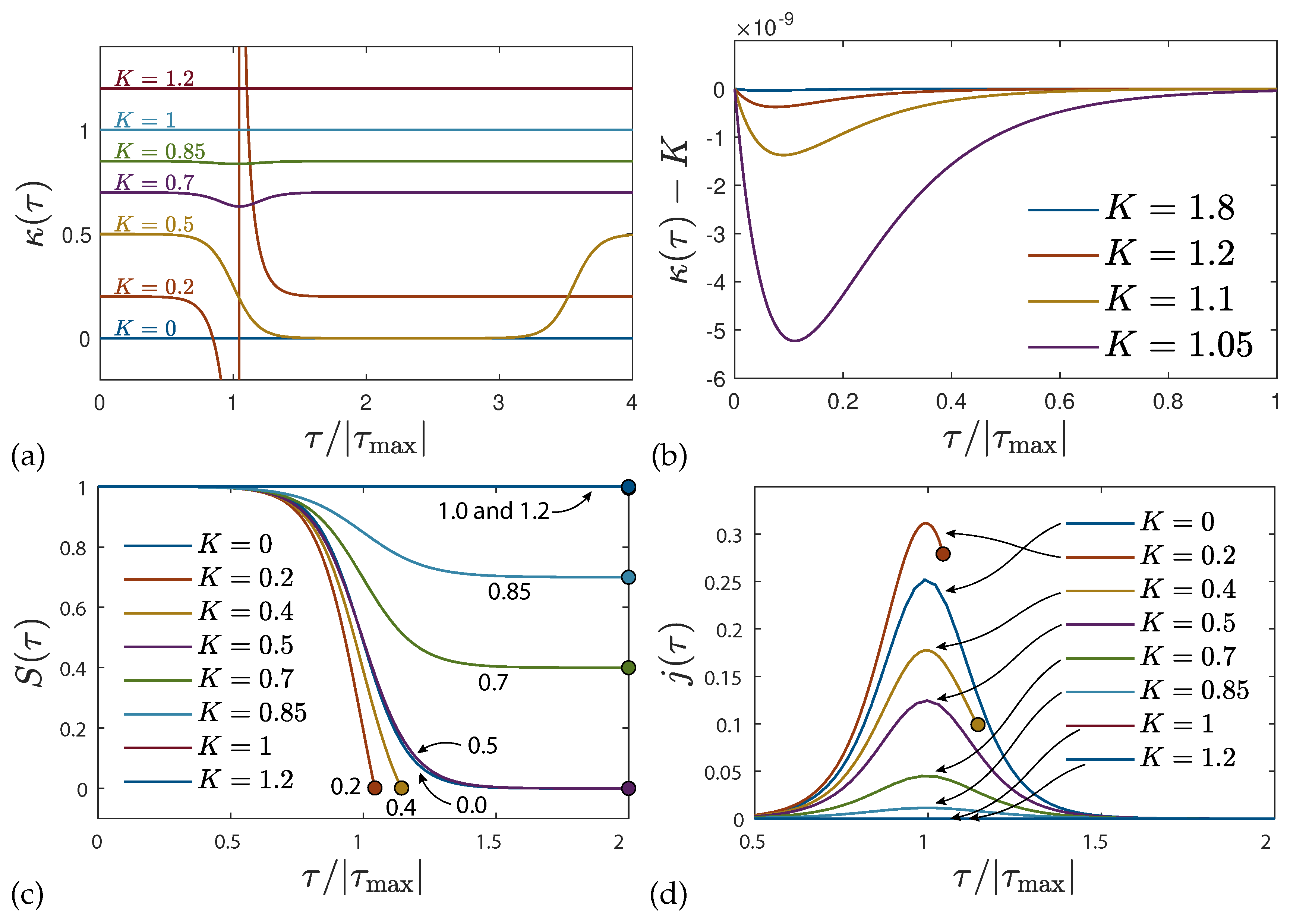
which are both shown in Figure 7 for different values of K entering

ρ (K)

and

τ_{0} (K)

. As

K \neq 0

the requirement

S (τ_{fin}) = 0

then provides from Equation (100)

(102)

where we used Equation (67) for

κ (0) = K

and inserted solution (87) for

0 < K \leq 2 K_{0}

. Obviously, positive values of

τ_{fin} (K)

are only possible for values of

K < 1

smaller then unity, as otherwise the argument of the

{tanh}^{- 1}

-function is negative. In order for the argument of the

{tanh}^{- 1}

-function to be less or equal unity the condition

\sqrt{{(K - K_{0})}^{2} + 2 η (1 - η)} \leq (1 + \frac{η}{2}) - K

(103)

is required, which is equivalent to

K \leq \frac{1}{2} .

(104)

Hence, finite values of

τ_{fin} (K)

only occur for values of

K \in (0, 0.5]

. In Figure 8 we show the final time (102) for different values of K below 0.5. The final time is monotonically decreasing from its infinitely large value above

K = 0.5

with decreasing values of K.

Particular interesting in Figure 7 are the cases where the combined ratio

κ (τ)

at the start and the end of the epidemic outburst have values below

K \leq 0.5

which corresponds to infection rates being twice as large as the sum of the recovery and fatality rate. In this case the epidemic outburst, described by the SI-type

{cosh}^{- 2} [(τ - τ_{\max}) / τ_{0}]

-distribution for the rate of new infections shown in panel Figure 7-d, is so dominated by the rapid infections that at the finite reduced time

τ_{fin}

the outburst suddenly terminates as with

S (τ_{fin}) = 0

(as seen in panel 7-c) no more persons are available to be infected. The situation is comparable to a smooth running car where suddenly the car engine stops as no more fuel is available. For values greater than

K > 0.5

the epidemic outburst lasts infinitely long.

Next, we consider the limits of Equations (101) and (102) for small values of

η ≪ 1

4.4. Limit for Very Small Values of $I (0) = η ≪ 1$

We use

\begin{matrix} tanh ρ (K) & = & \frac{K_{0} - K - \frac{η}{2}}{\sqrt{{(K - K_{0})}^{2} + 2 η (1 - η)} - \frac{η}{2}}, \end{matrix}

(105a)

\begin{matrix} τ_{0} (K) & = & \frac{2}{\sqrt{{(K - K_{0})}^{2} + 2 η (1 - η)} - \frac{η}{2}}, \end{matrix}

(105b)

and Equation (102). For small values of

η ≪ 1

we have to distinguish between the cases (i) where

| K - | K_{0} | \leq \sqrt{2 η}

and (ii) where

| K - K_{0} | > \sqrt{2 η}

. We consider both cases in turn.

4.4.1. Case $| K - K_{0} | \leq \sqrt{2 η}$

Here we approximate for small values of

η ≪ 1

\begin{matrix} \sqrt{{(K - K_{0})}^{2} + 2 η (1 - η)} - \frac{η}{2} & ≃ & \sqrt{2 η (1 - η)} [1 + \frac{{(K - K_{0})}^{2}}{2 η (1 - η)}] - \frac{η}{2} \\ ≃ & \sqrt{2 η} [1 + \frac{{(K - K_{0})}^{2}}{2 η} - \sqrt{\frac{η}{8}}] . \end{matrix}

(106)

Consequently, we obtain

\begin{matrix} tanh ρ (K) & ≃ & \frac{[1 - 2 η - K] [1 - \frac{{(K - K_{0})}^{2}}{2 η}]}{\sqrt{2 η}}, \end{matrix}

(107a)

\begin{matrix} τ_{0} (K) & ≃ & \sqrt{\frac{2}{η}} [1 - \frac{{(K - K_{0})}^{2}}{2 η}], \\ τ_{\max} (K) & ≃ & \sqrt{\frac{2}{η}} [1 - \frac{{(K - K_{0})}^{2}}{2 η}] {tanh}^{- 1} \frac{1 - 2 η - K}{\sqrt{2 η}} \end{matrix}

(107b)

\begin{matrix} = & \frac{1 - \frac{{(K - K_{0})}^{2}}{2 η}}{\sqrt{2 η}} ln \frac{\sqrt{2 η} + (1 - 2 η - K)}{\sqrt{2 η} - (1 - 2 η - K)}, \end{matrix}

(107c)

whereas

τ_{fin} = 0

as all K-values in this interval are greater than

0.5

4.4.2. Case $| K - K_{0} | > \sqrt{2 η}$

Here we approximate

\sqrt{{(K - K_{0})}^{2} + 2 η (1 - η)} - \frac{η}{2} ≃ | K_{0} - K | - \frac{η}{2} + \frac{η (1 - η)}{| K_{0} - K |},

(108)

to obtain for Equations (105) and (102)

\begin{matrix} tanh ρ (K) & ≃ & \frac{K_{0} - K - \frac{η}{2}}{| K - K_{0} | - \frac{η}{2} + \frac{η (1 - η)}{| K_{0} - K |}}, \end{matrix}

(109a)

\begin{matrix} τ_{0} (K) & ≃ & \frac{2}{| K_{0} - K | - \frac{η}{2} + \frac{η (1 - η)}{| K_{0} - K |}}, \end{matrix}

(109b)

\begin{matrix} τ_{fin} (K) & ≃ & \frac{2}{| K_{0} - K | - \frac{η}{2} + \frac{η (1 - η)}{| K_{0} - K |}} {tanh}^{- 1} [\frac{| K - K_{0} | - \frac{η}{2} + \frac{η (1 - η)}{| K_{0} - K |}}{1 - K}] . \end{matrix}

(109c)

4.4.3. Finite Time $τ_{fin} (K)$

As shown before, c.f. Equation (104), finite values of the finite time only occur for values of

K \leq 0.5 < K_{0}

. Consequently for small

η ≪ 1

we approximate with

K_{0} = 1 - (3 / 2) η

\begin{matrix} τ_{fin} (K) & ≃ & \frac{2}{K_{0} - K - \frac{η}{2} + \frac{η (1 - η)}{K_{0} - K}} {tanh}^{- 1} [\frac{K_{0} - K - \frac{η}{2} + \frac{η (1 - η)}{K_{0} - K}}{1 - K}] \\ = & \frac{2}{1 - K - 2 η + \frac{η (1 - η)}{K_{0} - K}} {tanh}^{- 1} [\frac{1 - K - 2 η + \frac{η (1 - η)}{K_{0} - K}}{1 - K}] \\ ≃ & \frac{2}{1 - K - \frac{η [2 (K_{0} - K) - 1]}{K_{0} - K}} {tanh}^{- 1} [1 - \frac{η [2 (K_{0} - K) - 1]}{(K_{0} - K) (1 - K)}] \\ = & \frac{1}{1 - K - \frac{η [2 (K_{0} - K) - 1]}{K_{0} - K}} ln [\frac{2 (K_{0} - K) (1 - K) - η [2 (K_{0} - K) - 1]}{η [2 (K_{0} - K) - 1]}] \\ ≃ & \frac{1}{1 - K} ln \frac{2 (K_{0} - K) (1 - K)}{η [2 (K_{0} - K) - 1]} . \end{matrix}

(110)

Equation (110) only provides real values if the denominator of the ln-function is positive, leading to the requirement

K < K_{0} - \frac{1}{2} = \frac{1 - 3 η}{2},

(111)

which is consistent with the earlier limit (104) and the time (110) can be further approximated as

τ_{fin} (K) ≃ \frac{1}{1 - K} ln \frac{2 {(1 - K)}^{2}}{η (1 - 2 K)} .

(112)

The function (112) monotonically decreases from its infinite large values above

(1 - η) / 2

with decreasing values of K in agreement with Figure 8.

4.4.4. Values $K < K_{0} - \sqrt{2 η}$

For values of

K < K_{0} - \sqrt{2 η}

one obtains

\begin{matrix} tanh ρ (K) & = & \frac{1}{1 + \frac{η (1 - η)}{(K_{0} - K) (K_{0} - K - \frac{η}{2})}} ≃ 1 - \frac{η (1 - η)}{{(K_{0} - K)}^{2}}, \end{matrix}

(113a)

\begin{matrix} τ_{0} (K) & ≃ & \frac{2}{K_{0} - K} [1 - \frac{η (2 + K - K_{0}}{2 {(K_{0} - K)}^{2}}], \end{matrix}

(113b)

\begin{matrix} τ_{\max} (K) & ≃ & \frac{1}{K_{0} - K} ln \frac{2 {(K_{0} - K)}^{2}}{η} . \end{matrix}

(113c)

With

{cosh}^{2} ρ = \frac{1}{1 - {tanh}^{2} ρ} = \frac{1}{1 - {[1 - \frac{η (1 - η)}{{(K_{0} - K)}^{2}}]}^{2}} ≃ \frac{{(K_{0} - K)}^{2}}{2 η (1 - η)}

(114)

Equation (101) becomes

\begin{matrix} κ (τ) & ≃ & 1 - η + (K_{0} - K) tanh (T - ρ) - \frac{2 η (1 - η)}{(K_{0} - K) (coth T - tanh ρ)} \\ - \frac{{(K_{0} - K)}^{2}}{2 (1 - η) {cosh}^{2} (T - ρ) [1 - \frac{2 η (1 - η)}{(K_{0} - K) (coth T - tanh ρ)}]}, \end{matrix}

(115)

which correctly approaches

κ (τ = 0) = 1 - η - (K_{0} - K) tanh ρ - \frac{{(K_{0} - K)}^{2}}{2 (1 - η) {cosh}^{2} ρ} ≃ 1 - (K_{0} - K) = K .

(116)

For values of

(1 - 3 η) / 2 < K < K_{0} - \sqrt{2 η}

we find

\begin{matrix} κ (τ = \infty) & = & 1 - η + K_{0} - K - \frac{2 η (1 - η)}{(K_{0} - K) [1 - tanh ρ]} \\ ≃ & 1 + K_{0} - K - 2 (K_{0} - K) = 1 - K_{0} + K = K, \end{matrix}

(117)

because for small

η ≪ 1

one has

K_{0} ≃ 1

. The solution (117) holds for all times

τ

in the range

(1 - 3 η) / 2 \leq K \leq K_{0} = 1 - (3 / 2) η - \sqrt{2 η}

. For smaller values of

K < (1 - 3 η) / 2

the solution (117) holds only at finite times

τ < τ_{fin} (K)

given in Equation (112).

4.4.5. Values $K_{0} + \sqrt{2 η} < K \leq 2 K_{0}$

For values of

K_{0} + \sqrt{2 η} < K \leq 2 K_{0}

we obtain

\begin{matrix} τ_{0} (K) & ≃ & \frac{2}{K - K_{0}}, \end{matrix}

(118a)

\begin{matrix} tanh ρ (K) & ≃ & - \frac{1}{1 + \frac{η}{K - K_{0} + \frac{η}{2}} \frac{1 + K_{0} - K - η}{K - K_{0}}} ≃ - [1 - \frac{η (1 + K_{0} - K)}{{(K - K_{0})}^{2}}], \end{matrix}

(118b)

\begin{matrix} τ_{\max} (K) & ≃ & - \frac{1}{K - K_{0}} ln \frac{2 {(K - K_{0})}^{2}}{η (1 + K_{0} - K)} \end{matrix}

(118c)

where the last step in Equation (118b) holds for values of

K < 2 - (5 η / 2)

, which is justified for all values of

K > K_{0}

as the maximum value

2 K_{0} = 2 - 3 η

is smaller than

2 - (5 η / 2)

. Consequently, one obtains in this case for

{cosh}^{2} ρ = \frac{1}{1 - {tanh}^{2} ρ} ≃ \frac{{(K - K_{0})}^{2}}{2 η (1 + K_{0} - K - η)},

(119)

so that

η (1 - η) τ_{0} {cosh}^{2} ρ ≃ \frac{(1 - η) (K - K_{0})}{1 + K_{0} - K} .

(120)

We also note that for

K > 1 - 2 η

the function

ρ (K) = - r (K)

in Equation (118b) is negative with

r (K) = {tanh}^{- 1} \frac{1}{1 + \frac{η}{K - K_{0} + \frac{η}{2}} \frac{1 + K_{0} - K - η}{K - K_{0}}} ≃ {tanh}^{- 1} [1 - \frac{η (1 + K_{0} - K)}{{(K - K_{0})}^{2}}],

(121)

so that Equations (101) or (61) become

\begin{matrix} κ (τ) & ≃ & \frac{2}{τ_{0}} tanh (T + r) + (1 - η) [1 - η τ_{0} {cosh}^{2} r (tanh (T + r) - tanh r)] \\ - \frac{η {cosh}^{2} r}{{cosh}^{2} (T + r) [1 - η τ_{0} {cosh}^{2} r (tanh (T + r) - tanh r)]} \\ ≃ & (K - K_{0}) tanh (T + r) + (1 - η) [1 - \frac{K - K_{0}}{1 + K_{0} - K} (tanh (T + r) - tanh r)] \\ - \frac{{(K - K_{0})}^{2}}{2 {cosh}^{2} (T + r) [1 + K_{0} - K - (K - K_{0}) (tanh (T + r) - tanh r)]} \end{matrix}

(122)

One notices from Figure 6 that

r (K) ≫ 1

is very large compared to unity, so that Equation (122) with

tanh (T + r) ≃ tanh r ≃ 1

and

{cosh}^{- 2} (T + r) ≃ 0

simplifies to the constant

κ (τ) ≃ K - K_{0} + 1 = K .

(123)

4.5. SIRD Solution for $κ (0) = 0$

For

κ (0) = 0

Equation (66) for

y = 2 / τ_{0}

reduces to

y^{2} - (κ_{\infty} - η) y = 1 - η - (1 - 2 η) κ_{\infty},

(124)

with the two solutions

\begin{matrix} y_{1} & = & \frac{1}{2} [κ_{\infty} - η + \sqrt{{(κ_{\infty} - 2 + 3 η)}^{2} + 8 η (1 - η)}], \end{matrix}

(125a)

\begin{matrix} y_{2} & = & \frac{1}{2} [κ_{\infty} - η - \sqrt{{(κ_{\infty} - 2 + 3 η)}^{2} + 8 η (1 - η)}] . \end{matrix}

(125b)

We restrict our analysis to the interesting range of values of

0 < κ_{\infty} < 2 - 3 η

(

κ_{\infty} = 0

was treated in Section 4.1 already) and investigate the limit of small

η ≪ 1

. We then approximate

\sqrt{{(2 - 3 η - κ_{\infty})}^{2} + 8 η (1 - η)} ≃ 2 - 3 η - κ_{\infty} + \frac{4 η (1 - η)}{2 - κ_{\infty} - 3 η},

(126)

implying

\begin{matrix} y_{1} & ≃ & 1 - 2 η \frac{1 - κ_{\infty}}{2 - κ_{\infty}}, \end{matrix}

(127a)

\begin{matrix} y_{2} & = & κ_{\infty} - 1 - \frac{η κ_{\infty}}{2 - κ_{\infty}}, \end{matrix}

(127b)

Accordingly,

\begin{matrix} τ_{0, 1} & ≃ & \frac{2}{1 - 2 η \frac{1 - κ_{\infty}}{2 - κ_{\infty}}} ≃ 2 [1 + 2 η \frac{1 - κ_{\infty}}{2 - κ_{\infty}}], \end{matrix}

(128a)

\begin{matrix} τ_{0, 2} & ≃ & \frac{2}{κ_{\infty} - 1} [1 + \frac{η κ_{\infty}}{(2 - κ_{\infty}) (κ_{\infty} - 1)}] . \end{matrix}

(128b)

τ_{0}

has to be positive the solution (128b) can only be used for values of

1 < κ_{\infty} < 2 - 3 η

For

κ (0) = 0

Equation (63) reads

τ_{\max} = τ_{0} {tanh}^{- 1} [(1 - 2 η) τ_{0} / 2]

. The two solutions (128) then provide

\begin{matrix} τ_{\max, 1} & ≃ & 2 [1 + 2 η \frac{1 - κ_{\infty}}{2 - κ_{\infty}}] {tanh}^{- 1} [1 - \frac{2 η}{2 - κ_{\infty}}] \end{matrix}

\begin{matrix} ≃ & [1 + 2 η \frac{1 - κ_{\infty}}{2 - κ_{\infty}}] ln \frac{2 - κ_{\infty} - η}{η} ≃ ln \frac{2 - κ_{\infty}}{η}, \\ τ_{\max, 2} & = & \frac{2}{κ_{\infty} - 1} [1 + \frac{η κ_{\infty}}{(2 - κ_{\infty}) (κ_{\infty} - 1)}] {tanh}^{- 1} [\frac{1 - 2 η}{κ_{\infty} - 1} (1 + \frac{η κ_{\infty}}{(2 - κ_{\infty}) (κ_{\infty} - 1)})] \end{matrix}

(129a)

\begin{matrix} ≃ & \frac{2}{κ_{\infty} - 1} {tanh}^{- 1} \frac{1}{κ_{\infty} - 1} . \end{matrix}

(129b)

The argument of the

{tanh}^{- 1}

has to be in the interval

(- 1, 1)

. The requirement

{(κ_{\infty} - 1)}^{- 1} > - 1

is fulfilled for every positive

κ_{\infty} > 1

. However, the requirement

{(κ_{\infty} - 1)}^{- 1} < 1

is only possible for values of

κ_{\infty} > 2

in contradiction to the earlier assumption

κ_{\infty} \leq 2 - 3 η

. Therefore the second solution

τ_{\max, 2}

and

τ_{0, 2}

cannot be used. The only possible solution is this range of

0 < κ_{\infty} \leq 2 - 3 η

\begin{matrix} τ_{0} (κ_{\infty}) & = & τ_{0, 1} (κ_{\infty}) ≃ 2 [1 + 2 η \frac{1 - κ_{\infty}}{2 - κ_{\infty}}], \end{matrix}

(130a)

\begin{matrix} τ_{\max} (κ_{\infty}) & = & τ_{\max, 1} = τ_{0} (κ_{\infty}) {tanh}^{- 1} [\frac{1 - 2 η}{2} τ_{0} (κ_{\infty})] ≃ ln \frac{2 - κ_{\infty}}{η}, \end{matrix}

(130b)

\begin{matrix} ρ (κ_{\infty}) & = & {tanh}^{- 1} [\frac{1 - 2 η}{2} τ_{0} (κ_{\infty})] = {tanh}^{- 1} [(1 - 2 η) (1 + 2 η \frac{1 - κ_{\infty}}{2 - κ_{\infty}})] . \end{matrix}

(130c)

Consequently we obtain

\begin{matrix} tanh ρ (κ_{\infty}) & = & 1 - \frac{2 η}{2 - κ_{\infty}} - 4 η^{2} \frac{1 - κ_{\infty}}{2 - κ_{\infty}} ≃ 1 - \frac{2 η}{2 - κ_{\infty}}, \end{matrix}

(131)

\begin{matrix} 1 - tanh ρ (κ_{\infty}) & ≃ & \frac{2 η}{2 - κ_{\infty}}, \end{matrix}

(132)

\begin{matrix} {cosh}^{2} ρ (κ_{\infty}) & ≃ & \frac{1}{1 - {[1 - \frac{2 η}{2 - κ_{\infty}}]}^{2}} ≃ \frac{2 - κ_{\infty}}{4 η} . \end{matrix}

(133)

One then obtains for Equation (61) in this case

\begin{matrix} κ (τ) & ≃ & \frac{2 tanh (T - ρ (κ_{\infty}))}{τ_{0} (κ_{\infty})} \\ + (1 - η) [1 - η τ_{0} (κ_{\infty}) {cosh}^{2} ρ (κ_{\infty}) [tanh (T - ρ (κ_{\infty})) + tanh ρ (κ_{\infty})]] \\ - \frac{η {cosh}^{2} ρ (κ_{\infty})}{{cosh}^{2} (T - ρ (κ_{\infty})) [1 - η τ_{0} (κ_{\infty}) (tanh (T - ρ (κ_{\infty})) + tanh ρ (κ_{\infty}))]} . \end{matrix}

(134)

Here, and in the following two equations, T and

ρ

stand for

τ / τ_{0} (κ_{\infty})

and

ρ (κ_{\infty}) = τ_{\max} (κ_{\infty}) / τ_{0} (κ_{\infty})

with

τ_{0} (κ_{\infty})

τ_{\max} (κ_{\infty})

, and

ρ (κ_{\infty})

given by Equations (130). The temporal evolution of

κ (τ)

is shown in Figure 9 for various values of

κ_{\infty} \in [0, 2]

. Equation (134) correctly reproduces

\begin{matrix} κ (τ = 0) & = & 1 - 2 η - \frac{2 tanh ρ}{τ_{0}} = 1 - 2 η - 2 \frac{1 - 2 η}{2} = 0, \\ κ (τ = \infty) & = & \frac{2}{τ_{0} (κ_{\infty})} + (1 - η) [1 - \frac{η τ_{0}}{1 - tanh ρ (κ_{\infty})})] \end{matrix}

(135)

\begin{matrix} ≃ & \frac{2}{τ_{0} (κ_{\infty})} + (1 - η) [1 - \frac{2 - κ_{\infty}}{2} τ_{0} (κ_{\infty})] ≃ κ_{\infty} \end{matrix}

(136)

with

τ_{0} (κ_{\infty}) ≃ 2

5. Approximate Analytical Solutions of the SIRVD Model

Recently, it has been demonstrated that an accurate analytical approximation to the SIR and SIRV equations[19] exists if the cumulative fraction of new infections

J (t) = J (τ)

at all times is much smaller than unity. For the COVID-19 outbreaks in many countries this assumption is well fulfilled.

According to Equation (19) in ref. [19] the approximation

1 - J (τ) ≃ 1 - J_{\infty}

in Equation (21) provides the solution

V (τ) ≃ (1 - J_{\infty}) [1 - e^{- \int_{0}^{τ} d x b (x)}],

(137)

which approaches

V_{\infty} = V (\infty) = 1 - J_{\infty}

after infinite time. With this result in the same limit

J \leq J_{\infty} ≪ 1

Equation (25) with the initial condition

j (0) = η (1 - η)

integrates

\begin{matrix} j (τ) & ≃ & η (1 - η) exp \int_{0}^{τ} d x [(1 - J_{\infty}) e^{- \int_{0}^{x} d y b (y)} - k (x) - q (x) - b (x)] \\ ≃ & η (1 - η) exp \int_{0}^{τ} d x [e^{- \int_{0}^{x} d y b (y)} - k (x) - q (x) - b (x)], \end{matrix}

(138)

where the last approximation holds due to the adopted smallness

J_{\infty} ≪ 1

. But we keep the

J_{\infty}

in the solution (137) in order not to violate the restriction

J (τ) + V (τ) \leq J_{\infty} + V_{\infty} \leq 1

. By integrating Equation (138) the corresponding cumulative fraction is given by

J (τ) ≃ η + η (1 - η) \int_{0}^{τ} d z exp [\int_{0}^{z} d x (e^{- \int_{0}^{x} d y b (y)} - k (x) - q (x) - b (x))] .

(139)

Likewise Equations (15) and (17)–(19) provide the approximations

I (τ) ≃ \frac{j (τ)}{1 - J_{\infty} - V (τ)} = \frac{η (1 - η)}{1 - J_{\infty}} exp \int_{0}^{τ} d x [e^{- \int_{0}^{x} d y b (y)} - k (x) - q (x)] = j (τ) e^{\int_{0}^{τ} d x b (x)},

(140)

R (τ) ≃ \int_{0}^{τ} d x \frac{k (x) j (x)}{1 - J_{\infty} - V (x)} = \frac{η (1 - η)}{1 - J_{\infty}} \int_{0}^{τ} d z k (z) exp \int_{0}^{z} d x [e^{- \int_{0}^{x} d y b (y)} - k (x) - q (x)],

(141)

D (τ) ≃ \int_{0}^{τ} d x \frac{q (x) j (x)}{1 - J_{\infty} - V (x)} = \frac{η (1 - η)}{1 - J_{\infty}} \int_{0}^{τ} d z q (z) exp \int_{0}^{z} d x [e^{- \int_{0}^{x} d y b (y)} - k (x) - q (x)],

(142)

and

\begin{matrix} d (τ) & = & \frac{d D (τ)}{d τ} = q (τ) I (τ) = \frac{q (τ) j (τ)}{1 - J_{\infty} - V (τ)} \\ ≃ & \frac{η (1 - η)}{1 - J_{\infty}} q (τ) exp \int_{0}^{τ} d x [e^{- \int_{0}^{x} d y b (y)} - k (x) - q (x)] . \end{matrix}

(143)

5.1. Difference between the SIRVD Death Rate and the a-Posteriori Death Rate

As it marks the difference of the death rate (143) in the SIRVD model to the a-posteriori death rate

d_{a - pos} (τ) = q (t) j (τ)

(34) we consider first the ratio

\frac{d_{a - pos} (τ)}{d (τ)} = \frac{j (τ)}{I (τ)} = S (τ) ≃ 1 - J_{\infty} - V (τ) = (1 - J_{\infty}) e^{- \int_{0}^{τ} d x b (x)} .

(144)

For the SIRD model with negligible vaccinations (

b (τ) = 0

), the ratio (144) is independent of reduced time and practically equals unity as

J_{\infty} ≪ 1

. However, for the SIRVD model including vaccinations the ratio (144) depends on time. The SIRVD death rate has a flatter

τ

-dependence than the a-posteriori death rate.

5.2. Conditions for Extrema

As before [19] it is straightforward to calculate the first and second time derivatives of the approximative solution (138) as

\begin{matrix} \frac{d j}{d τ} & = & η (1 - η) [e^{- \int_{0}^{τ} d y b (y)} - k (τ) - b (τ) - q (τ)] \times \end{matrix}

\begin{matrix} exp \int_{0}^{τ} d x [e^{- \int_{0}^{x} d y b (y)} - k (x) - b (x) - q (x)], \\ \frac{d^{2} j}{d τ^{2}} & = & η (1 - η) ({[e^{- \int_{0}^{τ} d y b (y)} - k (τ) - b (τ) - q (τ)]}^{2} - \frac{d k}{d τ} - \frac{d b}{d τ} - \frac{d q}{d τ} - b (τ) e^{- \int_{0}^{τ} d y b (y)}) \times \end{matrix}

(145a)

\begin{matrix} exp \int_{0}^{τ} d x [e^{- \int_{0}^{x} d y b (y)} - k (x) - b (x) - q (x)] . \end{matrix}

(145b)

Consequently, extrema of the rate of new infections occur at reduced times

τ_{E}

determined by

k (τ_{E}) + b (τ_{E}) + q (τ_{E}) = e^{- \int_{0}^{τ_{E}} d y b (y)} \leq 1,

(146)

where we indicate that the right-hand-side of this Equation is smaller than or equal to unity. Hence no extrema of infections occur for a sum of variations

k (τ) + b (τ) + q (τ_{E}) > 1 .

(147)

In the alternative case of reduced time intervals, where

k (τ) + b (τ) + q (τ_{E}) < 1,

(148)

extrema are possible. From Equation (145b) one obtains

\begin{matrix} {[\frac{d^{2} j}{d τ^{2}}]}_{τ_{E}} & = & - η (1 - η) ({[\frac{d k}{d τ}]}_{τ_{E}} + {[\frac{d b}{d τ}]}_{τ_{E}} + \frac{d q}{d τ}]_{τ_{E}} + b^{2} (τ_{E}) + b (τ_{E}) k (τ_{E}) + b (τ_{E}) q (τ_{E})) \times \\ exp [\int_{0}^{τ_{E}} d x (e^{- \int_{0}^{x} d y b (y)} - k (x) - b (x) - q (x))], \end{matrix}

(149)

Hence, the extrema are maxima if

{[\frac{d k}{d τ}]}_{τ_{E}} + {[\frac{d b}{d τ}]}_{τ_{E}} + \frac{d q}{d τ}]_{τ_{E}} + b^{2} (τ_{E}) + b (τ_{E}) k (τ_{E}) + b (τ_{E}) q (τ_{E}) > 0

(150)

is positive. They are minima if

{[\frac{d k}{d τ}]}_{τ_{E}} + {[\frac{d b}{d τ}]}_{τ_{E}} + \frac{d q}{d τ}]_{τ_{E}} + b^{2} (τ_{E}) + b (τ_{E}) k (τ_{E}) + b (τ_{E}) q (τ_{E}) < 0

(151)

is negative. There can be multiple minima and maxima depending on the reduced time variation of the ratios

k (τ)

and

b (τ)

. The extreme values of the rate of new infections are given by

j_{E} (τ_{E}) = η (1 - η) e^{\int_{0}^{τ_{E}} d x [e^{- \int_{0}^{x} d y b (y)} - k (x) - b (x) - q (x)]} .

(152)

All results given in this Section for the SIRVD model include as special cases the corresponding quantities in the SIRD model for

b (τ) = 0

and the SIR model for

b (τ) = q (τ) = 0

, respectively. The excellent agreement with the respective numerical solutions of the SIR and SIRV models [19] has proven the validity of the analytical approximation using the smallness of

J (τ) ≪ 1

6. SIRVD Model Applications

Next we illustrate our results from the preceding section with two examples. While Section 6.1 is concerned with the case of stationary ratios, in Section 6.3 we work out the case of a gradually decreasing fatality rate.

6.1. Stationary Ratios

We first consider the approximative solutions (137) and (138) in the special case of stationary ratios

\begin{matrix} k (τ) & = & k_{0}, \\ b (τ) & = & b_{0}, \\ q (τ) & = & q_{0} \end{matrix}

(153)

This case corresponds to the numerical solutions of the SIRVD model shown before in Figure 2.

If we introduce

κ_{0} = k_{0} + b_{0}

we may use the earlier results of ref.[19] to obtain

V (τ) = (1 - J_{\infty}) [1 - e^{- b_{0} τ}],

(154)

and

j (τ) = η (1 - η) exp [\frac{1 - e^{- b_{0} τ}}{b_{0}} - (κ_{0} + b_{0}) τ] .

(155)

Provided

κ_{0} + b_{0} = k_{0} + q_{0} + b_{0} < 1

, the rate of new infections (155) attains its maximum value

\begin{matrix} j_{\max} & = & j (τ_{m}) = η (1 - η) {(κ_{0} + b_{0})}^{\frac{κ_{0} + b_{0}}{b_{0}}} e^{\frac{1 - (κ_{0} + b_{0})}{b_{0}}} \\ = & η (1 - η) {(k_{0} + q_{0} + b_{0})}^{\frac{k_{0} + q_{0} + b_{0}}{b_{0}}} e^{\frac{1 - (k_{0} + q_{0} + b_{0})}{b_{0}}} . \end{matrix}

(156)

at the reduced time

τ_{m} = - \frac{ln (k_{0} + q_{0} + b_{0})}{b_{0}} .

(157)

For the cumulative fraction one finds

\begin{matrix} J (τ) & = & η + η (1 - η) b_{0}^{\frac{κ_{0}}{b_{0}}} e^{\frac{1}{b_{0}}} [γ (1 + \frac{κ_{0}}{b_{0}}, \frac{1}{b_{0}}) - γ (1 + \frac{κ_{0}}{b_{0}}, \frac{e^{- b_{0} τ}}{b_{0}})] \\ = & η + η (1 - η) b_{0}^{\frac{k_{0} + q_{0}}{b_{0}}} e^{\frac{1}{b_{0}}} [γ (1 + \frac{k_{0} + q_{0}}{b_{0}}, \frac{1}{b_{0}}) - γ (1 + \frac{k_{0} + q_{0}}{b_{0}}, \frac{e^{- b_{0} τ}}{b_{0}})] \end{matrix}

(158)

in terms of the lower incomplete gamma function

γ

. For infinitely large times, the fraction (158) approaches the final value

J_{\infty} = J (τ = \infty) = η + η (1 - η) b_{0}^{\frac{k_{0} + q_{0}}{b_{0}}} e^{\frac{1}{b_{0}}} γ (1 + \frac{k_{0} + q_{0}}{b_{0}}, \frac{1}{b_{0}}) .

(159)

Likewise, the SIRVD death rate (143) in this case becomes

d (τ) = \frac{d D (τ)}{d τ} ≃ η (1 - η) q_{0} exp [\frac{1 - e^{- b_{0} τ}}{b_{0}} - (k_{0} + q_{0}) τ] = q_{0} e^{b_{0} τ} j (τ) = e^{b_{0} τ} d_{a - pos} (τ) .

(160)

It differs from the a-posteriori death rate by the factor

e^{b_{0} τ}

reflecting the ratio between

I (τ)

and

j (τ)

. The rate (160) peaks at the time

τ_{d} = - \frac{ln (k_{0} + q_{0})}{b_{0}},

(161)

which is greater than the peak time

τ_{m}

of the rate of new infections, since

ln (x)

is monotonically increasing with increasing x. The maximum SIRVD death rate

d_{\max} = q_{0} η (1 - η) {(k_{0} + q_{0})}^{\frac{k_{0} + q_{0}}{b_{0}}} e^{\frac{1 - k_{0} - q_{0}}{b_{0}}} = \frac{e^{1}}{k_{0} + q_{0}} {[1 + \frac{b_{0}}{k_{0} + q_{0}}]}^{- [1 + \frac{k_{0} + q_{0}}{b_{0}}]} d_{\max}^{a - pos}

(162)

is smaller than the maximum a-posteriori death rate.

The corresponding cumulative fraction of fatalities is given by

D (τ) = q_{0} η (1 - η) b_{0}^{\frac{k_{0} + q_{0} - b_{0}}{b_{0}}} e^{\frac{1}{b_{0}}} [γ (\frac{k_{0} + q_{0}}{b_{0}}, \frac{1}{b_{0}}) - γ (\frac{k_{0} + q_{0}}{b_{0}}, \frac{e^{- b_{0} τ}}{b_{0}})],

(163)

with the final value

D_{\infty} = D (τ = \infty) = q_{0} η (1 - η) b_{0}^{\frac{k_{0} + q_{0} - b_{0}}{b_{0}}} e^{\frac{1}{b_{0}}} γ (\frac{k_{0} + q_{0}}{b_{0}}, \frac{1}{b_{0}})

= \frac{q_{0} η (1 - η)}{k_{0} + q_{0}} [b_{0}^{\frac{k_{0} + q_{0}}{b_{0}}} e^{\frac{1}{b_{0}}} γ (1 + \frac{k_{0} + q_{0}}{b_{0}}, \frac{1}{b_{0}}) + 1] .

(164)

It has been shown before in Equation (57) of ref. [19] that for small values of

b_{0} ≪ 1

and

b_{0} < κ_{0} = k_{0} + q_{0} < 1

the cumulative fractions as well as their final values have to be calculated with the leading order approximation for large values of

z ≫ 1

z^{- κ_{0} z} γ (1 + κ_{0} z, z) ≃ \sqrt{2 π κ_{0} z} κ_{0}^{κ_{0} z} e^{- κ_{0} z} - e^{- z} .

(165)

Applying this approximation to Equations (159) and (164) with

z = b_{0}^{- 1}

provides

\begin{matrix} J_{\infty} & ≃ & η (1 - η) [\sqrt{\frac{2 π (k_{0} + q_{0})}{b_{0}}} e^{\frac{1 - (k_{0} + q_{0})}{b_{0}}} {(k_{0} + q_{0})}^{\frac{k_{0} + q_{0}}{b_{0}}} - 1], \end{matrix}

(166a)

\begin{matrix} D_{\infty} & ≃ & \frac{q_{0} η (1 - η)}{k_{0} + q_{0}} \sqrt{\frac{2 π (k_{0} + q_{0})}{b_{0}}} e^{\frac{1 - (k_{0} + q_{0})}{b_{0}}} {(k_{0} + q_{0})}^{\frac{k_{0} + q_{0}}{b_{0}}} ≃ \frac{1}{k_{0} + q_{0}} D_{\infty}^{a - pos} . \end{matrix}

(166b)

We note that the ratio

D_{\infty} / D_{\infty}^{a - pos}

does not depend on the value of

b_{0}

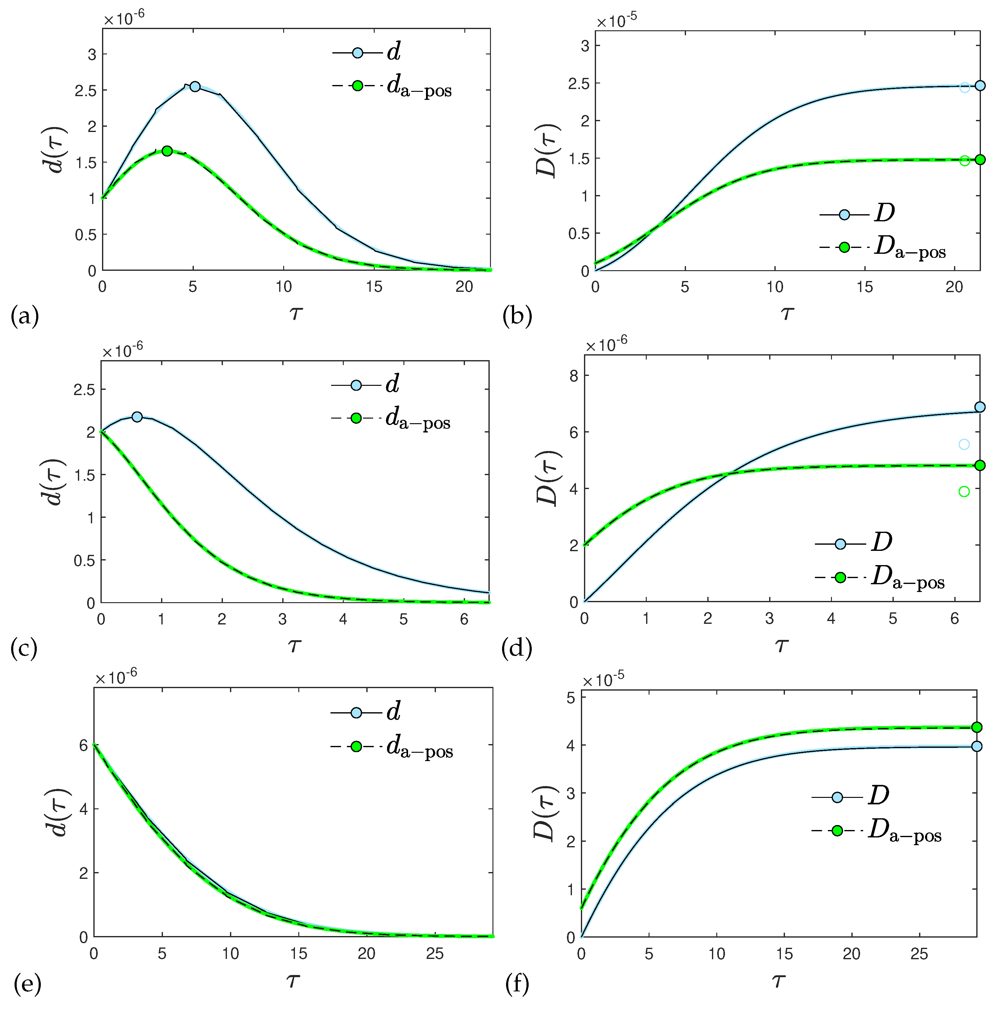
These differences are clearly seen in the panels of Figure 10. The SIR, SIRV and SIRD curves, representing a-posteriori death rates, have a significant different reduced time dependence compared to the SIRVD curve. For

b_{0} ≪ k_{0} + q_{0} < 1

one infers from Eqs. (158) and (161),

\frac{τ_{m}}{τ_{d}} = 1 + \frac{ln (1 + \frac{b_{0}}{k_{0} + q_{0}})}{ln (k_{0} + q_{0})} ≃ 1 + \frac{b_{0}}{(k_{0} + q_{0}) ln (k_{0} + q_{0})} < 1 .

(167)

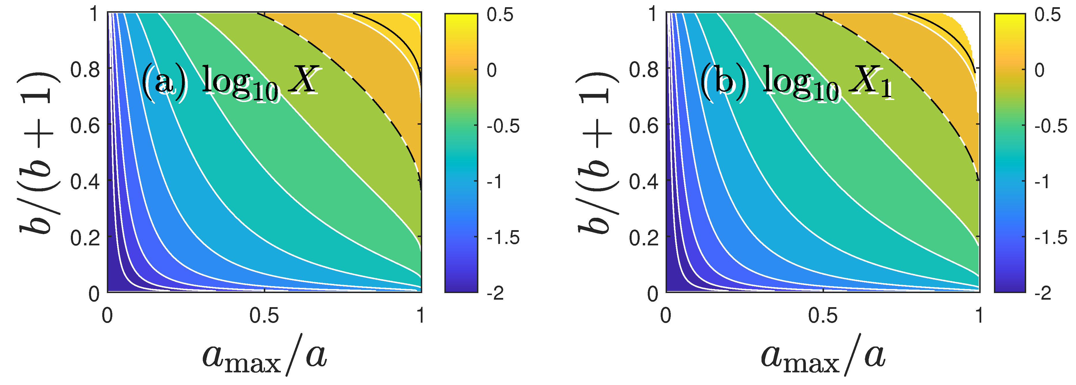
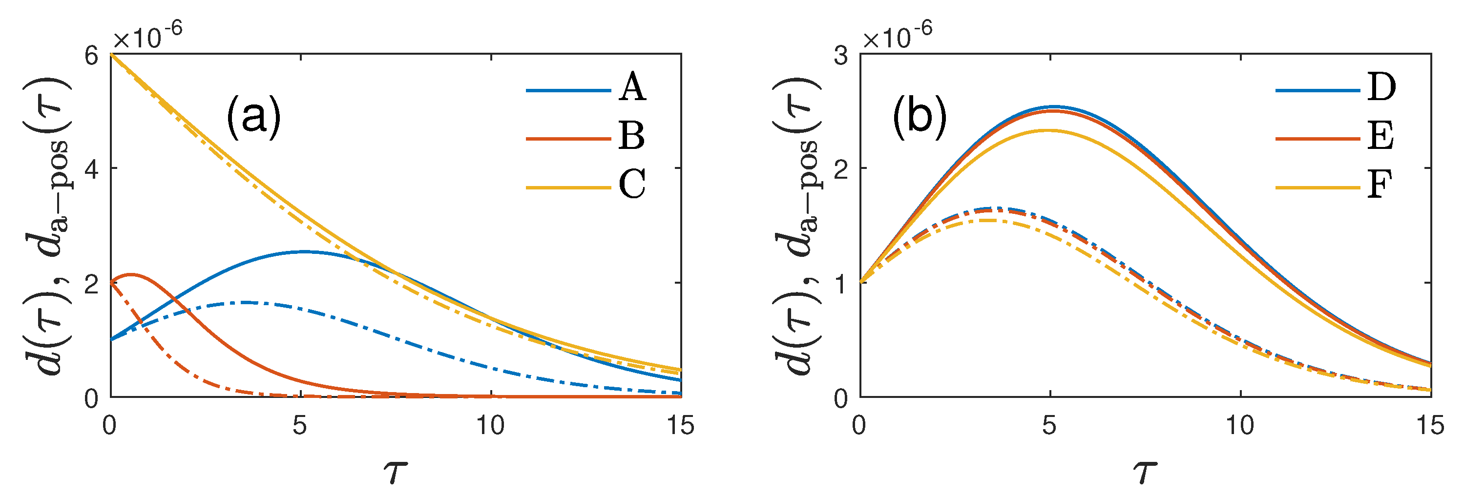
For the values of

k_{0} = 0.5

b_{0} = 0.1

and

q_{0} = 0.1

shown in Figure 10-a,b, the maximum death rate is a factor

1.54

smaller than the maximum a-posteriori death rate, the final cumulative fraction of fatalities is a factor

1.67

larger than its a-posteriori value, and the death rate peaks at the later time

τ_{d} = 5.1

as compared to the peak time

τ_{m} = 3.6

of the a-posteriori death rate. For this example the exact numerical ratio is

τ_{m} / τ_{d} \approx 0.69

, to be compared with

\approx 0.67

from the analytical expression (167). The performance of the analytical solution

j (τ)

(155) of the SIRVD model over a wide range of its determining parameters

κ_{0}

and

b_{0}

is analyzed in Figure 11.

6.2. Application to Measured COVID-19 Data

Here we exemplify on how to obtain all SIRVD model parameters from measured COVID-19 data of a completed pandemic wave, if all rates are considered time-independent. Using results from the foregoing section, we are going to demonstrate how to extract all parameters analytically from a few characteristics contained in the reported data.

To this end we collected data capturing the first pandemic COVID-19 wave for several countries. Usually, only the cumulative number of newly infected persons,

N J (t)

and the cumulative number of deceased persons,

N D (t)

are reported, while the population size N can be considered known. Sometimes,

R (t)

is reported as well, but typically useless, as not all recovered persons report their recovery, and

R (t)

is then simply estimated based on

J (t)

and

D (t)

. Note, that the current fraction of infected population,

I (t)

, as well as the susceptible population fraction,

S (t)

, are usually not measurable.

We thus rely on the reported

J (t)

and

D (t)

time series as function of time t, as well as their derivatives

\overset{˚}{J} = d J / d t

and

\overset{˚}{D} = d D / d t

, starting at the time

t = 0

of the outbreak, which we define here to coincide with the day at which 10 persons have been infected so far,

N J (0) = 10

. The most robust quantities that can be obtained from such time series are the final plateau values

J_{\infty}

and

D_{\infty}

, when

\overset{˚}{J}

and

\overset{˚}{D}

approached zero or a value that is very small compared with the peak values

{\overset{˚}{J}}_{\max}

and

{\overset{˚}{D}}_{\max}

of the measured rates. As proven in Appendix D the following procedure can be followed: (i) calculate the ratio

G \in (0, 1)

defined in Equation (A41), i.e.,

G = \frac{{\overset{˚}{D}}_{\max} J_{\infty}}{{\overset{˚}{J}}_{\max} D_{\infty} e},

(168)

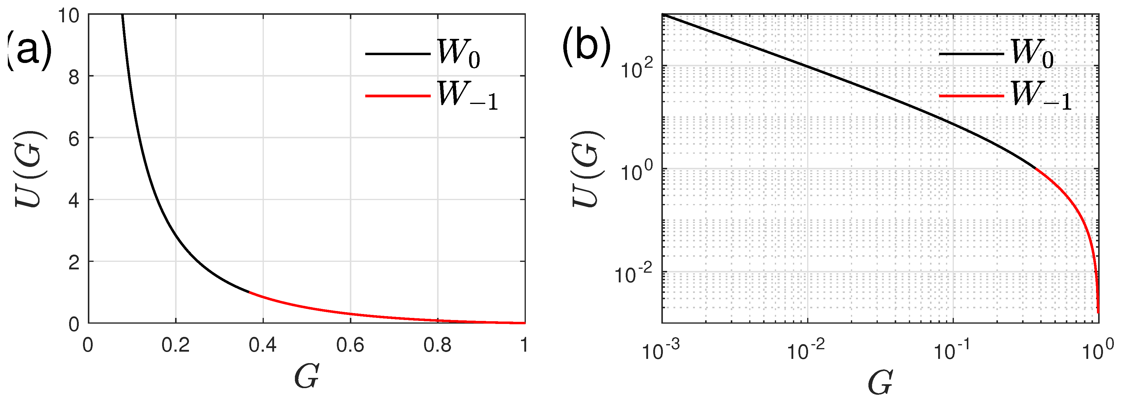
(ii) calculate a real-valued, positive U with the help of Lambert’s W function,

\begin{matrix} U & = & \frac{ln G}{W_{0} (G ln G)} (G \leq e^{- 1}), \end{matrix}

(169)

\begin{matrix} U & = & \frac{ln G}{W_{- 1} (G ln G)} (G \geq e^{- 1}), \end{matrix}

(170)

where the choice of principal versus non-principal branch depends on the magnitude of G. While Lambert’s W function is routinely available in engineering software, Figure 12 can alternatively be used to look up U for given G, (iii) with U and the three measured ratios

t_{d} / t_{m}

D_{\infty} / J_{\infty}

{\overset{˚}{D}}_{\max} / {\overset{˚}{J}}_{\max}

at hand, calculate

κ_{0} = U^{- t_{d} / (t_{d} - t_{m})}

(171)

according to Equation (A41), (iv) obtain the three dimensionless SIRVD rates via Equation (A37), i.e.,

q_{0} = κ_{0} \frac{D_{\infty}}{J_{\infty}}, k_{0} = κ_{0} - q_{0}, b_{0} = κ_{0}^{t_{m} / t_{d}} - κ_{0} .

(172)

Finally, the dimensional rates, if needed, are given by Equations (10) and (157),

a_{0} = - \frac{ln (κ_{0} + b_{0})}{t_{m} b_{0}}, μ_{0} = a_{0} k_{0}, v = a_{0} b_{0}, ψ = a_{0} q_{0},

(173)

since

a_{0} = τ_{m} / t_{m}

. This procedure had been followed to create Table 1 for a few selected countries, for which the assumption

κ_{0} + q_{0} < 1

underlying the present treatment apply, using public available data [23]. With the parameters at hand, the time-evolution not only of the reported, but also of the remaining compartments S, R and V is predicted by the SIRVD model.

The outlined simple recipe must not produce the best possible fit to the measured data by any measure, but it ensures that the three characteristic values are exactly reproduced. Moreover, in an analogous fashion it is possible to use the analytic solution to efficiently extract the SIRVD parameters from measured data well before peak times have been reached, for example using polynomial coefficients of the time series, ratios between cumulative fractions at different times etc. This allows to forecast the evolution of all compartments.

6.3. Gradually Decreasing Fatality Rate

Here we investigate the approximative solutions (137) and (138) in the special case of stationary ratios

k (τ) = k_{0}

b (τ) = b_{0}

but the gradually decreasing fatality rate

q (τ) = q_{0} - q_{1} (1 - e^{- G τ})

(174)

with constants

q_{0}

q_{1}

and G. The fatality rate (174) starts from the constant value

q_{0}

and decreases with the typical time scale

G^{- 1}

to its final constant value

q_{1}

. Such a behavior accounts well for the COVID-19 omicron which had a much smaller (about an order of magnitude) fatality rate than the earlier mutants occurring about a year earlier. Such a slow gradual decrease is well captured by the adopted fatality rate (174) in the case

G ≪ b_{0} < 1

, allowing us the linear approximation

q (τ \leq G^{- 1}) ≃ q_{0} - q_{1} G τ,

(175)

if necessary.

The vaccination rate (154) is independent from the fatality rate

q (τ)

and also applies here, whereas with the rate (174) the rate of new infections (138) becomes

j (τ) ≃ η (1 - η) exp [\frac{1 - e^{- b_{0} τ}}{b_{0}} - (k_{0} + b_{0} + q_{0} - q_{1}) τ - q_{1} \frac{1 - e^{- G τ}}{G}] .

(176)

Consequently, one finds for Equations (140)–(143)

\begin{matrix} I (τ) & = & j (τ) e^{b_{0} τ} ≃ η (1 - η) exp [\frac{1 - e^{- b_{0} τ}}{b_{0}} - (k_{0} + q_{0} - q_{1}) τ - q_{1} \frac{1 - e^{- G τ}}{G}], \end{matrix}

(177a)

\begin{matrix} R (τ) & ≃ & k_{0} I (τ) = η (1 - η) k_{0} exp [\frac{1 - e^{- b_{0} τ}}{b_{0}} - (k_{0} + q_{0} - q_{1}) τ - q_{1} \frac{1 - e^{- G τ}}{G}], \\ d (τ) & = & [q_{0} - q_{1} (1 - e^{- G τ})] η (1 - η) exp [\frac{1 - e^{- b_{0} τ}}{b_{0}} - (k_{0} + q_{0} - q_{1}) τ - q_{1} \frac{1 - e^{- G τ}}{G}], \end{matrix}

(177b)

(177c)

and

D (τ) ≃ η (1 - η) \int_{0}^{τ} d z [q_{0} - q_{1} (1 - e^{- G z})] exp [\frac{1 - e^{- b_{0} z}}{b_{0}} - (k_{0} + q_{0} - q_{1}) z - q_{1} \frac{1 - e^{- G z}}{G}],

(178)

respectively, whereas the cumulative fraction of infections is given by

J (τ) ≃ η + η (1 - η) \int_{0}^{τ} d z exp [\frac{1 - e^{- b_{0} z}}{b_{0}} - (k_{0} + b_{0} + q_{0} - q_{1}) z - q_{1} \frac{1 - e^{- G z}}{G}] .

(179)

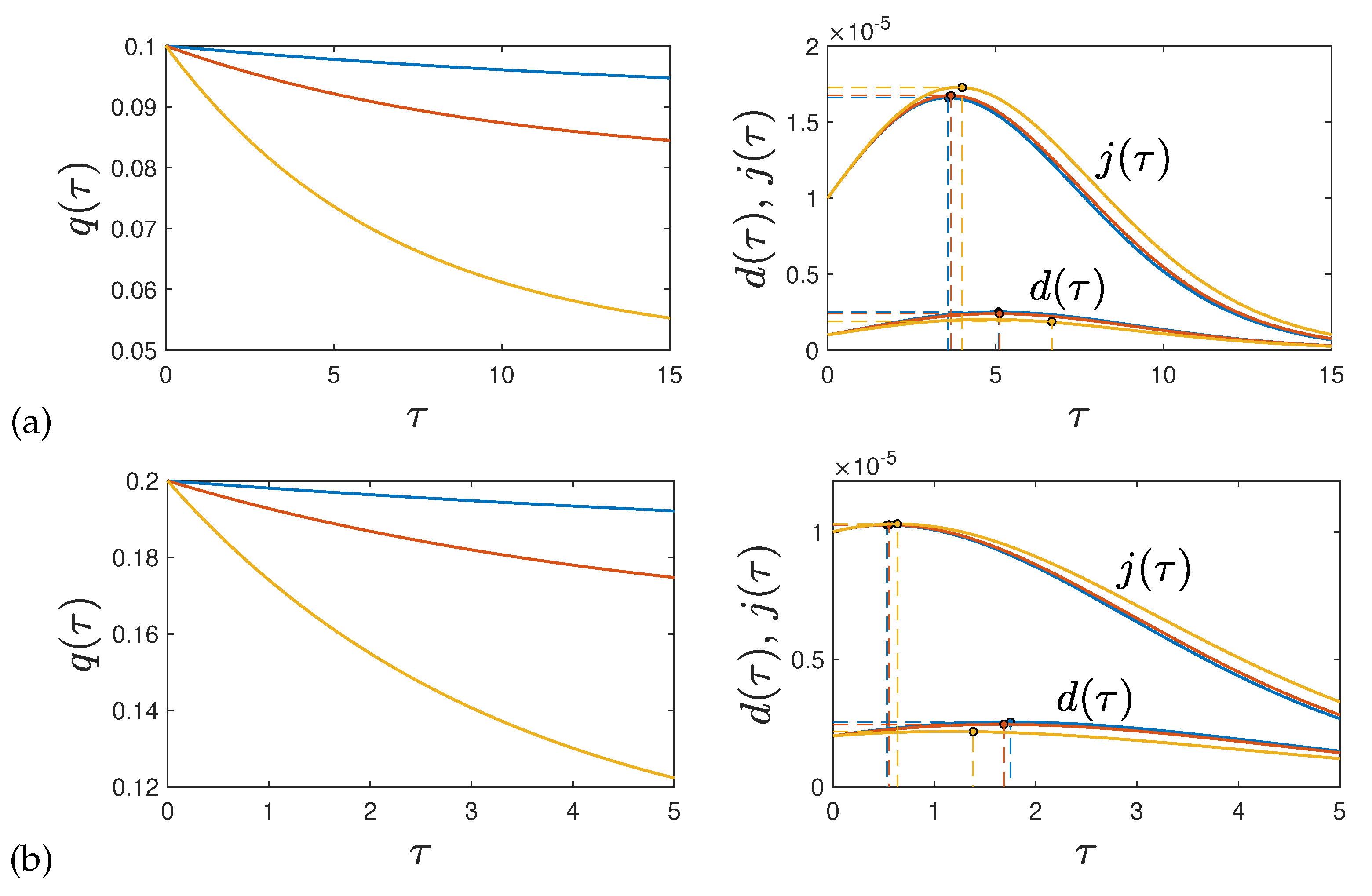
The analytical expressions are in excellent agreement with the numerical solutions of the SIRVD model in the presence of time-dependent

q (τ)

. In Figure 13 we show selected results for

j (τ)

and

d (τ)

, while all other quantities are equally well captured.

6.3.1. Peak Times

For values of

k_{0} + b_{0} + q_{0} < 1

the rate of new infections (176) peaks at the time given by

e^{- b_{0} τ_{m}} - q_{1} e^{- G τ_{m}} = k_{0} + b_{0} + q_{0} - q_{1},

(180)

whereas the death rate (177c) attains its maximum at

τ_{d}

determined by

[q_{0} - q_{1} (1 - e^{- G τ_{d}})] [e^{- b_{0} τ_{d}} - k_{0}] - q_{1} (G + 2 q_{0} - 2 q_{1}) e^{- G τ_{d}} - {(q_{0} - q_{1})}^{2} - q_{1}^{2} e^{- 2 G τ_{d}} = 0

(181)

Both Equations (180)–(181) are nonlinear and cannot be solved in closed form2. However, if we use, as in Equation (175), the approximation

e^{- G τ_{m . d}} ≃ 1 - G τ_{m, d}

Equations (180)–(181) can be approximated as

e^{- b_{0} τ_{m}} ≃ - q_{1} G τ_{m} + C_{0}, C_{0} = k_{0} + b_{0} + q_{0},

(182)

and

(q_{0} - q_{1} G τ_{d}) e^{- b_{0} τ_{d}} = q_{0} (k_{0} + q_{0}) + q_{1} G - q_{1} G (k_{0} + 2 q_{0} + G) τ_{d} .

(183)

This latter equation (183), treated below, is of the form of Wright’s transcendental equation. It is easy to see that Equations (176)–(183) in the limit

q_{1} = 0

correctly reduce to the earlier results in Section 6.1. The applicability of Equations (182) and (183) requires

G ≪ b_{0}

. Introducing the positive

z_{m} = b_{0} τ_{m}

and the positive combination

a_{m} = b_{0} C_{0} / q_{1} G

of parameters, the first Equation (182) reads

e^{- z_{m}} = C_{0} [1 - (z_{m} / a_{m})]

and thus determines

z_{m}

in terms of

a_{m}

and

C_{0}

. This latter equation is solved in terms of the non-principal Lambert function

W_{- 1}

(see Appendix G in ref. [25]) as

z_{m} = a_{m} + W_{- 1} (- \frac{e^{- 1 / a_{m}}}{a_{m} C_{0}}), τ_{m} = \frac{C_{0}}{q_{1} G} + \frac{1}{b_{0}} W_{- 1} (- \frac{b_{0} e^{- b_{0} C_{0} / q_{1} G}}{q_{1} G}),

(184)

where we have just re-inserted

z_{m}

and

a_{m}

in the second part of Equation (184).

As detailed in Appendix C the solution of Equation (183) is more involved. As for the calculation of

τ_{m}

, it is helpful to introduce a dimensionless time

z_{d} = b_{0} τ_{d}

, and to simplify Equation (183) using an appropriate combination of the five semipositive parameters

k_{0}

b_{0}

q_{0}

q_{1}

, G, and

z_{d}

. As shown in Appendix C it is possible to write Equation (183) in the form of Wright’s transcendental equation,

e^{- X} = 1 - \frac{2 b}{b - a - X},

(185)

or equivalently

a = - X - b coth (X / 2)

(186)

upon introducing X, a, and b via

\begin{matrix} X & = & z_{d} + ln C_{1}, C_{1} = k_{0} + 2 q_{0} + G, \\ a & = & b - \frac{b_{0} q_{0}}{q_{1} G} - ln C_{1}, \\ b & = & \frac{q_{0} + (1 - q_{1} / q_{0}) G}{2 C_{1}} \frac{b_{0} q_{0}}{q_{1} G}, \end{matrix}

(187)

Since

q_{1} < q_{0}

to ensure positive

q (τ)

, one has

b > 0

. Further,

a < 0

since

G ≪ b_{0}

. For positive values of b and negative values of a, no solutions to Equation (186) with negative X are possible. This is most easily seen by rewriting this equation as

a + X = b coth (X / 2)

. For negative X, the right hand side is negative, while left hand side is positive. Equation (186) hence implies

X > 0

, and

z_{d} > 0

implies

X > ln C_{1}

. The equation (185) is equivalent to Wright’s transcendental equation and known [26] to exhibit real-valued solutions X only for a limited range of a and b values. Using the x-parametric form of the envelope

a = - x - sinh (x)

and

b = - 1 + cosh (x)

[26] we derive the condition

a \leq - \sqrt{b} \sqrt{2 + b} - {cosh}^{- 1} (1 + b) \equiv a_{\max} \leq 0

(188)

for the existence of a

τ_{d}

value. The

a_{\max}

monotonically decreases with increasing b, starting from

a_{\max} = 0

and

b = 0

In Appendix C we obtain the following approximations for the exact solution of Equation (186):

\begin{matrix} X_{0} & ≃ & \frac{b - a}{2} [1 - \sqrt{1 - \frac{8 b}{{(b - a)}^{2}}}] ≃ \frac{2 b}{b - a}, (X \in [0, 1]) \end{matrix}

(189a)

\begin{matrix} X_{1} & ≃ & - \frac{3 a + \sqrt{9 a^{2} - 12 b (6 + b)}}{6 + b} (X \in [0, 2], a < - \frac{2 \sqrt{b (6 + b)}}{\sqrt{3}}, \end{matrix}

(189b)

\begin{matrix} X_{2} & ≃ & \frac{a^{2} - b^{2}}{2 b} + W_{- 1} (- \frac{{(a - b)}^{2} e^{- (a^{2} - b^{2}) / 2 b}}{2 b}), (X < b - a) \end{matrix}

(189c)

Note that

X_{0}

approaches unity for

a = a_{\max}

and

b \to \infty

, while

X_{2} \to \infty

behaves correctly in this limit. As detailed in Appendix C,

X_{0}

ist most precise for sufficiently small a well below

a_{\max}

X_{1}

performs extremely well (Figure 14) over the whole a-b range except very close to

a = a_{\max}

and large b, while

X_{2}

has advantages only in the regime where

X_{1}

fails. To summarize,

τ_{d}

exists as long as

a < a_{\max}

, and is then well approximated by

τ_{d} ≃ \frac{X_{1} - ln (k_{0} + 2 q_{0} + G)}{b_{0}}

(190)

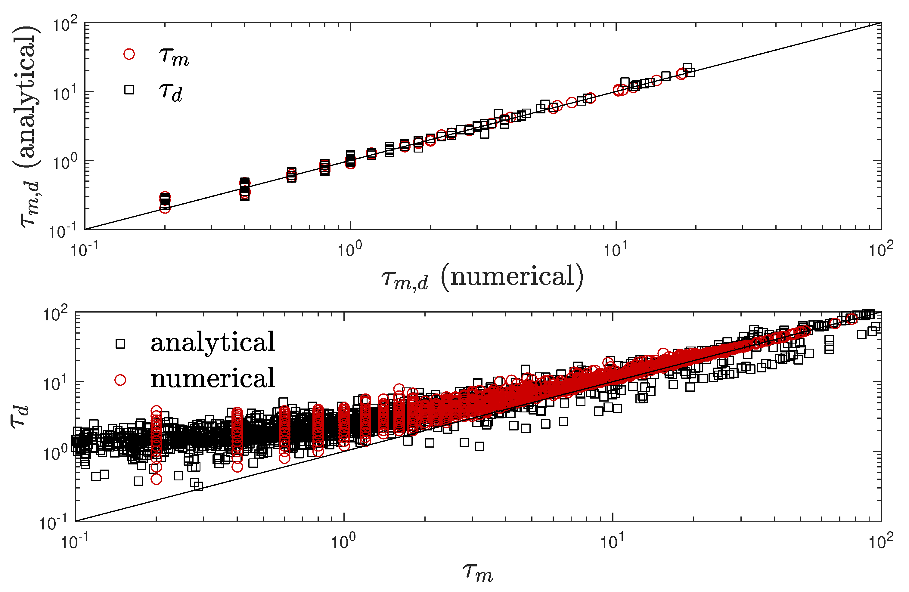
with a and b expressed in terms of

k_{0}

b_{0}

q_{0}

q_{1}

, and G via Equation (187). In Figure 13 we mark the analytical

τ_{m}

and

τ_{d}

for a few cases. As visible, they capture the peak times of the analytical solutions for

j (τ)

(176) and

d (τ)

(177c), that moreover are indistinguishable from the numerical solution. Since it is impossible to visualize the performance of the numerical versus analytical results for the case of time-dependent

q (τ)

, characterized by 6 parameters

k_{0}

b_{0}

q_{0}

q_{1}

, G, and

η

, we have randomly chosen sets of parameters with

k_{0}

q_{0}

b_{0} \in [0, 1]

q_{0} \in [0, q_{1}]

G \in [0, b_{0}]

, and

η \in [10^{- 7}, 10^{- 3}

]. The comparison is undertaken in Figure 15.

6.3.2. Maximum Rate of New Infections and Death Rate

With the peak times (184) and (190) inserted in Equations (176) and (177c), respectively, the maximum rates of the new infections and the maximum death rates are given by

\begin{matrix} j_{\max} & = & η (1 - η) e^{\frac{1 - k_{0} - b_{0} - q_{0} + q_{1}}{b_{0}} - \frac{q_{1}}{G}} exp [\frac{q_{1} (b_{0} - G)}{b_{0} G} e^{- G τ_{m}} - (k_{0} + b_{0} + q_{0} - q_{1}) τ_{m}] \\ ≃ & η (1 - η) e^{\frac{1 - k_{0} - b_{0} - q_{0} + q_{1}}{b_{0}} - \frac{q_{1}}{G}} exp [\frac{q_{1} (b_{0} - G)}{b_{0} G} e^{- \frac{k_{0} + b_{0} + q_{0}}{q_{1}} - \frac{G}{b_{0}} W_{- 1} (- \frac{b_{0} e^{- b_{0} (k_{0} + b_{0} + q_{0}) / q_{1} G}}{q_{1} G}}) \\ - (k_{0} + b_{0} + q_{0} - q_{1}) [\frac{k_{0} + b_{0} + q_{0}}{q_{1}} + \frac{1}{b_{0}} W_{- 1} (- \frac{b_{0} e^{- b_{0} (k_{0} + b_{0} + q_{0}) / q_{1} G}}{q_{1} G})]], \end{matrix}

(191)

where we made use of the determining Equation (180), and

\begin{matrix} d_{\max} & = & [q_{0} - q_{1} (1 - e^{- G τ_{d}})] η (1 - η) e^{\frac{1}{b_{0}} - \frac{q_{1}}{G}} exp [- \frac{e^{- b_{0} τ_{d}}}{b_{0}} - (k_{0} + q_{0} - q_{1}) τ_{d} + \frac{q_{1} e^{- G τ_{d}}}{G}] \\ = & [q_{0} - q_{1} (1 - {(k_{0} + 2 q_{0} + G)}^{\frac{G}{b_{0}}} e^{- \frac{G X_{1}}{b_{0}}})] η (1 - η) e^{\frac{1}{b_{0}} - \frac{q_{1}}{G}} exp [- \frac{(k_{0} + 2 q_{0} + G) e^{- X_{1}}}{b_{0}} \\ - \frac{k_{0} + q_{0} - q_{1}}{b_{0}} (X_{1} - ln (k_{0} + 2 q_{0} + G) + \frac{q_{1}}{G} {(k_{0} + 2 q_{0} + G)}^{\frac{G}{b_{0}}} e^{- \frac{G X_{1}}{b_{0}}}] . \end{matrix}

(192)

6.3.3. Death Rates

In Figure 16 we compare the death rate (177c) and the a-posteriori death rate (34)

d_{a - pos} (τ) = [q_{0} - q_{1} (1 - e^{- G τ})] j (τ),

(193)

with

j (τ)

from Equation (176) for six different choices of parameters. In each case the analytical death rates agree very well with the corresponding numerical solutions of the SIRVD model proving the accuracy of the analytical approximation.

We observe earlier peak-times for the a-posteriori death rates, following the rate

j (τ)

of newly infected individuals, compared with the SIRVD death rate

d (τ)

, following

I (τ)

. Additionally, the SIRVD death rates are significantly larger compared with those obtained through the a-posteriori treatment, with direct implications for the corresponding

D_{\infty}

values. Our predictions for these differences are suitable for being corroborated with past monitored pandemic data on the rate of new infections and the death rates of sufficient quality with negligible underestimation i.e. negligible dark numbers.

7. Summary and Conclusions

We have investigated a special class of exact solutions as well as accurate analytical approximations of the SIRVD and SIRD compartment models. For nonlinear models with a high-dimensional parameter space analytical solutions, exact or accurately approximative, are of high importance and interest: not only as suitable benchmarks for numerical codes, but especially as they allow us to understand the critical behavior of epidemic outbursts as well as the decisive role of certain parameters [27]. For given reduced time variations of the ratios

k (τ)

q (τ)

and

b (τ)

the SIRVD and SIRD equations represent complicated integro-differential equations for the rate of new infections

j (τ)

as well as the cumulative fraction of infections

J (τ)

, or

S (τ)

and

I (τ)

. However, the integro-differential equations can also be regarded as simpler determining equations for the sum of ratios

k (τ) + q (τ) = κ (τ)

for given variations of the ratio

b (τ)

and the fraction

S (τ)

. This new approach has been used to derive fully exact analytical solutions for the SIRVD and SIRD models. Especially for the SIRD model it is an effective new method to construct a special class of exact solutions depending on two parameters which are chosen as the values of the ratio

κ (τ)

at the start (

κ (τ = 0)

) and the end (

κ (τ = \infty

κ (τ)

at the start and the end of the epidemic outburst have values below

K \leq 0.5

which corresponds to infection rates being twice as large as the sum of the recovery and fatality rate. In this case the epidemic outburst, described by the SI-type

{cosh}^{- 2} [(τ - τ_{\max}) / τ_{0}]

-distribution for the rate of new infections, is so dominated by the rapid infections that at the finite reduced time

τ_{fin}

the outburst suddenly terminates as with

S (τ_{fin}) = 0

no more persons are available to be infected. The situation is comparable to a smooth running car where suddenly the car engine stops as no more fuel is available. For values greater than

K > 0.5

the epidemic outburst lasts until infinitely large times.

In the second part of the manuscript the recently developed analytical approximation [19] for the SIR and SIRV models are applied to the more general SIRVD model. In the limit of small cumulative fractions

J ≪ 1

, which very often is fulfilled, this approximation provides accurate analytical expressions for all epidemic quantities of interest such as the rate of new infections

\overset{˚}{J} (t)

and the fraction

I (t)

of infected persons. One of the referees has kindly informed us that our analytical approach is related to the Perov’s fixed point theorem [28]. As an aside, when determining

τ_{d}

in Appendix C we provided accurate approximative solutions to Wright’s transcendental equation (A16), or equivalently, Equation (185). The main difference of the SIRVD to the SIRV model is the discrimination between recovered and deceased persons by introducing two different compartments which affects the calculation of the death rate. In the SIRVD/SIRD cases it is proportional to

I (t)

, whereas in many SIR models in an a-posteriori approach it is proportional to

\overset{˚}{J} (t)

. It is shown that the temporal dependence of

I (t)

and

\overset{˚}{J} (t)

are different when the effect of vaccinations is included and/or when the real time dependence of the fatality rate

ψ (t)

and the recovery rate

μ (t)

are different from each other. We illustrate these pronounced differences with two applications: one for stationary ratios

k_{0}

b_{0}

and

q_{0}

, and one for stationary ratios

k_{0}, b_{0}

but a gradually decreasing fatality rate. In our analysis, we observe earlier peak-times for the rate of newly infected individuals compared with death rates. Additionally, our findings indicate significantly smaller death rates compared with those obtained through the a-posteriori treatment. We are hopeful that these differences can be corroborated with past monitored pandemic data on the rate of new infections and the death rates of sufficient quality, with negligible underestimation. We didn’t account for the widely acknowledged 7-day delay between the onset of infection and the resulting death. This delay impacts both the death rate in our SIRVD model and the subsequent a-posteriori death rate analysis in a consistent manner. As a result, the derived difference in peak times remains unchanged. The case of stationary ratios allows one to construct a new powerful diagnostics method to extract analytically all SIRVD model parameters from measured COVID-19 data of a completed pandemic wave. The new diagnostics method is applied to the monitored COVID-19 data in four countries. Potential future work on this subject should include (1) incorporating in the SIRVD model spatially heterogeneous situations by adding spatial diffusion, (2) a detailed testing of the predictions with suitable data from past COVID-19 waves also for time-dependent ratios

k (τ)

q (τ)

and

b (τ)

, and (3) the derivations of accurate mathematical approximation for more complicated time variations of the ratios

k (τ)

q (τ)

and

b (τ)

Author Contributions

Conceptualization, R.S.; Methodology, R.S. and M.K.; Formal analysis, M.K. and R.S.; Writing—original draft, R.S.; Writing—review & editing, M.K.; Visualization, M.K.. All authors have read and agreed to the published version of the manuscript.

Funding

This research received no external funding.

Data Availability Statement

All data are enclosed with this publication.

Acknowledgments

We acknowledge support by chatgpt in rephrasing the abstract, and removing all mathematical symbols from our version.

Conflicts of Interest

The authors declare no conflicts of interest.

Appendix A. SI Model

In the case of vanishing

k (τ) = q (τ) = b (τ) = 0

the SIRVD equations (11a)–(11f) reduce to

\begin{matrix} \frac{d S}{d τ} & = & - S I, \end{matrix}

(A1a)

\begin{matrix} \frac{d I}{d τ} & = & S I, \end{matrix}

(A1b)

\begin{matrix} 1 & = & S (τ) + I (τ), \end{matrix}

(A1c)

subject to initial conditions

I (0) = η = 1 - S (0)

. Equation (A1b) provides

S = d ln I / d τ

, so that the sum constraint (A1c) reads

\frac{d I (τ)}{d τ} = I (τ) - I^{2} (τ) .

(A2)

Equation (A2) leads to the integral

τ = \int_{η}^{I} \frac{d z}{z - z^{2}} = \int_{\frac{1}{I}}^{\frac{1}{η}} \frac{d y}{y - 1} = ln \frac{\frac{1}{η} - 1}{\frac{1}{I} - 1},

(A3)

where we substituted

z = 1 / y

. Equation (A3) provides

\begin{matrix} I (τ) & = & \frac{1}{1 + \frac{1 - η}{η} e^{- τ}} \end{matrix}

(A4a)

\begin{matrix} S (τ) & = & 1 - I (τ) = \frac{1}{1 + \frac{η}{1 - η} e^{τ}} . \end{matrix}

(A4b)

The rate of new infections is then given by

\begin{matrix} j (τ) & = & S (τ) I (τ) = \frac{1}{2 + \frac{η}{1 - η} e^{τ} + \frac{1 - η}{η} e^{- τ}} \\ = & \frac{1}{2 [1 + cosh (τ - ln \frac{1 - η}{η})]} = \frac{1}{4 {cosh}^{2} [\frac{τ - ln \frac{1 - η}{η}}{2}]}, \end{matrix}

(A5)

to which we refer as the SI-type new infection rate in the main text.

Appendix B. Integro-Differential Equation for the SIRD Model

Here we consider the case of no vaccinations, i.e.

v = b = 0

and

V (τ) = 0

. In some aspects the resulting SIRD-model is simpler than the SIRVD-model, e.g. here the simpler relation

J (τ) = 1 - S (τ)

holds. This facilitates the general integro-differential equations (26)–(30) derived for the more general SIRVD model. Here, Equation (25) reduces to

κ (τ) = 1 - J (τ) - \frac{d}{d τ} ln [\frac{j (τ)}{1 - J (τ)}],

(A6)

where

κ (τ) = k (τ) + q (τ) .

(A7)

With the initial conditions Equation (A6) integrates to

\frac{j (τ)}{1 - J (τ)} = - \frac{d}{d τ} ln (1 - J (τ)) = η exp \int_{0}^{τ} d z [1 - J (z) - κ (z)],

(A8)

or alternatively

j (τ) = η e^{- \int_{0}^{τ} d z κ (z)} \frac{d}{d τ} e^{τ - \int_{0}^{τ} d z J (z)} = η [1 - J (τ)] e^{\int_{0}^{τ} d z [1 - κ (z) - J (z)]} .

(A9)

In terms of

S (τ) = 1 - J (τ)

in this case Equation (A8) reads

\frac{d ln S (τ)}{d τ} = \frac{d S (τ) / d τ}{S (τ)} = - η exp \int_{0}^{τ} d z [S (z) - κ (z)],

(A10)

which with the initial condition

S (τ = 0) = 1 - η

integrates to

S (τ) = (1 - η) exp [- η \int_{0}^{τ} d x exp (\int_{0}^{x} d z [S (z) - κ (z)])] .

(A11)

By writing

S = e^{ln S}

the last equation provides

ln \frac{S}{1 - η} = - \int_{0}^{τ} d x H (x) e^{\int_{0}^{x} d z S (z)},

(A12)

with the function

H (x) = e^{ln η - \int_{0}^{x} d z κ (z)}

. Equation (A11) is equivalent to

J (τ) = 1 - (1 - η) exp [- η \int_{0}^{τ} d x exp (\int_{0}^{x} d z [1 - J (z) - κ (z)])],

(A13)

whereas Equation (A10) can be written as

e^{\int_{0}^{τ} d z κ (z)} \frac{d S}{d τ} = - η \frac{d}{d τ} e^{\int_{0}^{τ} d z S (z)} .

(A14)

Equation (A9) yields for Equations (15), (17)–(19) in the SIRD case

\begin{matrix} I (τ) & = & \frac{j (τ)}{1 - J (τ)} = η e^{\int_{0}^{τ} d z [1 - κ (z) - J (z)]}, \end{matrix}

(A15a)

\begin{matrix} R (τ) & = & η \int_{0}^{τ} d x k (x) e^{\int_{0}^{x} d z [1 - κ (z) - J (z)]}, \end{matrix}

(A15b)

\begin{matrix} D (τ) & = & η \int_{0}^{τ} d x q (x) e^{\int_{0}^{x} d z [1 - κ (z) - J (z)]}, \end{matrix}

(A15c)

\begin{matrix} d (τ) & = & \frac{d D (τ)}{d τ} = q (τ) I (τ) = η q (τ) e^{\int_{0}^{τ} d z [1 - κ (z) - J (z)]}, \end{matrix}

(A15d)

respectively. Equations (A8)–(A10) represent the exact solutions for the SIRD and SIR equations for

κ = k (τ) + q (τ) = k_{tot}

. The only difference between these two occurs for the calculation of the fractions of recovered and removed persons. The integral equation (A12) cannot be solved analytically for

S (τ)

in general, but for

η ≪ 1

we show in Section 4 that an analytic solution exists within a range of

k_{tot}

values.

Appendix C. Solution of Wright’s Transcendental Equation

With

z = - b_{0} τ_{d}

Equation (183) is equivalent with Wright’s [26] transcendental equation

(q + p z) e^{z} = r z + s,

(A16)

with

q = q_{0} > 0

p = q_{1} G / b_{0} > 0

r = q_{1} G [k_{0} + 2 q_{0} + G] / b_{0} > 0

and

s = q_{0} (k_{0} + q_{0}) + q_{1} G > 0

and we follow Wright’s arguments, while he focused on the roots of Equation (A16). Because

p r \neq 0

we substitute

z = Z - ln (p / r) = Z + ln (k_{0} + 2 q_{0} + G),

(A17)

providing for Equation (A16)

(Z - a + b) e^{Z} = Z - a - b

(A18)

with the real-valued constants

\begin{matrix} a & = & - \frac{1}{2} (\frac{s}{r} + \frac{q}{p}) + ln (\frac{p}{r}) = - ln (k_{0} + 2 q_{0} + G) - \frac{b_{0} q_{0}}{q_{1} G} + b, \end{matrix}

(A19a)

\begin{matrix} b & = & - \frac{1}{2} (\frac{s}{r} - \frac{q}{p}) = \frac{b_{0} q_{0}}{q_{1} G} \frac{q_{0} + (1 - q_{1} / q_{0}) G}{2 (k_{0} + 2 q_{0} + G)} . \end{matrix}

(A19b)

This confirms Equation (187). Note that for

a = b = 0

the Equation (A18) is solved by

Z = 0

. To arrive at Equations (A16) and (A19a) we assumed

G τ_{d} ≪ 1

. While

b > 0

, for sufficiently small

G / b_{0}

the a is negative, more precisely, as soon as

\frac{G}{b_{0}} < - \frac{q_{0}}{q_{1}} \frac{1 - q_{0} / [2 (k_{0} + 2 q_{0} + G)]}{ln (k_{0} + 2 q_{0} + G)} .

(A20)

Because a can be assumed negative, we introduce the positively valued

A = b - a = \frac{q}{p} - ln (\frac{p}{r}) = ln (k_{0} + 2 q_{0} + G) + \frac{b_{0} q_{0}}{q_{1} G},

(A21)

so that

a = - (A - b)

. Equation (A18) then becomes

e^{Z} = 1 - \frac{2 b}{Z + A} .

(A22)

It is evident that Equation (A22) has no solutions for positive values of

Z > 0

, as its left-hand side is always larger than unity in that case while the right-hand side is smaller than unity. For negative values of

Z = - X

with

X > 0

Equation (A22) reads

e^{- X} = 1 - \frac{2 b}{A - X},

(A23)

and the substitution

X = A y

in Equation (A23) yields

e^{- A y} = 1 - \frac{2 b}{A (1 - y)},

(A24)

which only has solutions for

y < 1

because b is positive. Equation (A24) will be used below to derive approximants

X_{0}

and

X_{1}

, while approximant

X_{2}

considers Equation (A18) as the starting point. In deriving the approximants it will turn out important to recall that a fulfills the inequality

a < a_{\max} \leq 0

with

a_{\max}

given by Equation (188). An important limiting feature is

{lim}_{b \to 0} a_{\max} = 0

Appendix C.1. Derivation of X 0

Expanding

e^{- A y} ≃ 1 - A y

, which requires

y \leq A^{- 1}

(or

X \leq 1

) we obtain from Equation (A24)

y (y - 1) ≃ - \frac{2 b}{A^{2}},

(A25)

with the two solutions

\begin{matrix} y_{1} & = & \frac{1 - \sqrt{1 - 8 b / A^{2}}}{2} ≃ \frac{2 b}{A^{2}}, \end{matrix}

(A26a)

\begin{matrix} y_{2} & = & \frac{1 + \sqrt{1 - 8 b / A^{2}}}{2} ≃ 1 - \frac{2 b}{A^{2}} . \end{matrix}

(A26b)

Because

2 b / A^{2} ≪ 1

, since

\frac{2 b}{A^{2}} \leq \frac{2 b}{{(b - a_{\max})}^{2}} \leq lim_{b \to 0} \frac{2 b}{{(b - a_{\max})}^{2}} = lim_{b \to 0} (\frac{1}{4} - \frac{\sqrt{b}}{4 \sqrt{2}}) = \frac{1}{4},

(A27)

only the solution

y_{1}

fulfils the requirement

y_{1} \leq A^{- 1}

, corresponding to

(2 b / A) \leq 1

which is a valid inequality, as

\frac{2 b}{A} = \frac{2 b}{b - a} \leq \frac{2 b}{b - a_{\max}} = \frac{2 b}{b + \sqrt{b (2 + b) + {cosh}^{- 1} (1 + b)}} \leq 1 .

(A28)

The inequality (A27) therefore also implies that the argument under the square root is positive,

1 - 8 b / A^{2} > 0

. With

X_{0} = A y_{1} < 1

and

A = b - a

this completes the derivation of

X_{0}

in Equation (189a).

Appendix C.2. Derivation of X 2

Because

y < 1

, here we assume

y ≪ 1

and use the approximation

{(1 - y)}^{- 1} ≃ 1 + y

in Equation (A24) to obtain

e^{- A y} ≃ - \frac{2 b}{A} (y + 1 - \frac{A}{2 b}),

(A29)

with the solution

y = \frac{A}{2 b} - 1 + \frac{1}{A} W_{- 1} (- \frac{A^{2}}{2 b e^{A (\frac{A}{2 b} - 1)}}),

(A30)

where

W_{- 1}

is the non-principal branch of Lambert’s W function. For

a < a_{\max}

stated in Equation (188), the argument of the Lambert function is negative, decreases with increasing b, and resides within the interval

[- 1 / e, 0]

so that

W_{- 1}

is real-valued and

W_{- 1} < - 1

holds. The principal branch

W_{0}

of Lambert’s function solves Equation (A29) as well, but can be ruled out by considering the limit

b \to 0

and

a \to a_{\max}

. In this limit the argument of Lambert’s function evaluates, with

A = b - a

, to

lim_{b \to 0} - \frac{{(b - a_{\max})}^{2}}{2 b e^{(b - a_{\max}) (\frac{(b - a_{\max})}{2 b} - 1)}} = - \frac{4}{e^{4}} .

(A31)

On the other hand

lim_{b \to 0} \frac{{(b - a_{\max})}^{2}}{2 b} - b + a_{\max} = 4 .

(A32)

For the argument stated in Equation (A31), Lambert’s functions evaluate to

W_{0} (- 4 / e^{4}) \approx - 0.079

and

W_{- 1} (- 4 / e^{4}) = - 4

, respectively. Since we know that

X = A y = 0

solves Equation (A23) in the same limit, the principal branch

W_{0}

can be ruled out. With

X_{2} = A y ≪ A

this completes the derivation of

X_{2}

in Equation (189c).

Appendix C.3. Derivation of X 1

Equation (A18), technically divided by

e^{Z} - 1

, can also be written as

a = Z + b coth (\frac{Z}{2}) .

(A33)

Here we depart from Wright’s arguments and solve Equation (A33) with asymptotic expansions of the coth-function. For values of

| Z | \leq 2

we approximate

coth (Z / 2) ≃ 2 / Z [1 + (Z^{2} / 12)]

, so that in this range Equation (A33) reduces to the quadratic

(1 + \frac{b}{6}) Z^{2} - a Z + 2 b = 0,

(A34)

with the two solutions

Z_{\pm} = \frac{3 a \pm \sqrt{9 a^{2} - 12 b (6 + b)}}{6 + b} .

(A35)

The term under the square root is not strictly semipositive for any

a < a_{\max}

, but

Z_{\pm}

is real-valued for

a < - 2 \sqrt{b (6 + b) / 3}

, which is only slightly below

a_{\max}

; for

b < 10

it is only 3% below

a_{\max}

, giving rise to the tiny white region in top right corner of Figure A1. For this reason the question about the suitable sign in Equation (A35) cannot be answered by considering the limit

b \to 0

and

a \to a_{\max}

, as before. Instead, consider the following: Inserting

a = Z + χ sinh (Z)

and

b = χ [cosh (Z) - 1]

solves Equation (A33) for any choice of

χ

, i.e., one can write

a = Z - \sqrt{b (b + 2 χ)}, Z = - {cosh}^{- 1} (\frac{b + χ}{χ}),

(A36)

for positive

χ

. Using

χ = 1

we had derived

a_{\max}

. Using

χ = 0

in Equation (A36) yields

b = 0

and

a = Z

, while the 2nd relation in Equation (A36) in this limit is just the identity

Z = Z

. Inserting this special case of

a = Z

and

b = 0

into Equation (A35) yields

Z_{\pm} = (Z \pm Z) / 2

. As we expect to find

Z_{\pm} = Z

, the suitable solution is

Z_{+}

. With

X_{1} = - Z_{+} < 2

this completes the derivation of

X_{1}

in Equation (189b).

Figure A1. Top row from left to right: The exact solution X to Equation (185) or (186) versus

a_{\max} / a

and

b / (b + 1)

with the negative

a_{\max}

defined by Equation (188), approximants

X_{0, a}

X_{0, b}

X_{1}

, and

X_{2}

given by Equation (189). For any X and b, the exact solution corresponds to

a = - X - b coth (X / 2)

according to Equation (186). Two contourlines are highlighted in each panel, if they exist:

X = 1

(dashed black) and

X = 2

(solid black). In the

X_{1}

panel, the

X_{1}

is undefined in the small white region in the top right corner, defined by

a < - 2 \sqrt{b (6 + b) / 3}

. In the

X_{2}

panel, the

X_{2}

cannot be evaluated numerically in the yellow region which is characterized by

X > 1

and

a > a_{\max} / 2

. Bottom row from left to right: The relative deviation

Δ X

between approximants

X_{0, a}

X_{0, b}

X_{1}

and

X_{2}

and the exact numerical solution X, again versus

a_{\max} / a

and

b / (b + 1)

. The color scale ranges from blue (relative deviation below 1%, to yellow (relative deviation above 10%). Approximant

X_{1}

performs very well except in the tiny top right corner (large b, a close to

a_{\max}

), where

X_{2}

has some advantage.

Figure A1. Top row from left to right: The exact solution X to Equation (185) or (186) versus

a_{\max} / a

and

b / (b + 1)

with the negative

a_{\max}

defined by Equation (188), approximants

X_{0, a}

X_{0, b}

X_{1}

, and

X_{2}

given by Equation (189). For any X and b, the exact solution corresponds to

a = - X - b coth (X / 2)

according to Equation (186). Two contourlines are highlighted in each panel, if they exist:

X = 1

(dashed black) and

X = 2

(solid black). In the

X_{1}

panel, the

X_{1}

is undefined in the small white region in the top right corner, defined by

a < - 2 \sqrt{b (6 + b) / 3}

. In the

X_{2}

panel, the

X_{2}

cannot be evaluated numerically in the yellow region which is characterized by

X > 1

and

a > a_{\max} / 2

. Bottom row from left to right: The relative deviation

Δ X

between approximants

X_{0, a}

X_{0, b}

X_{1}

and

X_{2}

and the exact numerical solution X, again versus

a_{\max} / a

and

b / (b + 1)

. The color scale ranges from blue (relative deviation below 1%, to yellow (relative deviation above 10%). Approximant

X_{1}

performs very well except in the tiny top right corner (large b, a close to

a_{\max}

), where

X_{2}

has some advantage.

Appendix D. Recipe for Stationary Rates

In Section 6.2 we showed how to extract all SIRVD model parameters from reported data. Here we derive the required relationships. For stationary infection rates

a (t) = a_{0}

the reduced time is defined by

τ = a_{0} t

as we have adopted without loss of generality

t = 0

as the start of the pandemic wave; in other words,

t_{m}

and

t_{d}

are peak times with respect to the day of the outbreak. Equation (167) then provides

b_{0} = κ_{0}^{t_{m} / t_{d}} - κ_{0}

(A37)

which is positive for

t_{d} > t_{m}

. We also use the approximation

J_{\infty} / D_{\infty} ≃ κ_{0} / q_{0}

(166b) so that

q_{0} ≃ κ_{0} \frac{D_{\infty}}{J_{\infty}} .

(A38)

So far we have expressed

b_{0}

and

q_{0}

in terms of measurable ratios and

κ_{0}

. Equations (156) and (162) provide for a third measurable ratio

\frac{{\overset{˚}{J}}_{\max}}{{\overset{˚}{D}}_{max}} = \frac{κ_{0}}{q_{0} e} {(1 + \frac{b_{0}}{κ_{0}})}^{1 + \frac{κ_{0}}{b_{0}}} = \frac{J_{\infty}}{D_{\infty} e} {(1 + \frac{b_{0}}{κ_{0}})}^{1 + \frac{κ_{0}}{b_{0}}},

(A39)

where we inserted Equation (A38). Inserting Equation (A37) then converts Equation (A39) into a closed nonlinear equation determining

κ_{0}

G U^{\frac{U}{U - 1}} = 1,

(A40)

where we introduced the quantities

U = κ_{0}^{\frac{t_{m}}{t_{d}} - 1}, G = \frac{{\overset{˚}{D}}_{\max} J_{\infty}}{{\overset{˚}{J}}_{\max} D_{\infty} e} .

(A41)

Taking the logarithm of Equation (A40) leads to

ln G + \frac{U}{U - 1} ln U = 0 .

(A42)

For

U \neq 1

we multiply (A42) with

U - 1

to obtain

(U - 1) ln G + U ln U = 0,

(A43)

U [ln U + ln G] = ln G .

(A44)

Setting

F = U G = \frac{{\overset{˚}{D}}_{\max} J_{\infty}}{{\overset{˚}{J}}_{\max} D_{\infty} e} κ_{0}^{\frac{t_{m}}{t_{d}} - 1}

(A45)

one can cast Equation (A44) into the form

F ln F = G ln G .

(A46)

The trivial solution

F = G

, corresponding to

U = 1

, is excluded as we adopted

U \neq 1

above. The remaining useful solution of Equation (A46) is

F = \frac{G ln G}{W (G ln G)}

(A47)

in terms of the Lambert’s W function. In light of the following basic features of the principal (

W_{0}

) and non-principal (

W_{- 1}

) branches of the W function [29],

\begin{matrix} W_{0} (G ln G) & = & ln G, G \geq e^{- 1}, \\ W_{- 1} (G ln G) & = & ln G, G \leq e^{- 1}, \end{matrix}

(A48)

that absorb the mentioned trivial solution, the relevant nontrivial solution is given by the remaining (opposite) regimes:

W_{0}

for large, and

W_{- 1}

for small G. Recalling

F = U G

, the solution of Equation (A40) is therefore given by Equation (170) stated in the main text.

References

Bailey, N.T. The Mathematical Theory of Infectious Diseases and its Applications; Charles Griffin & Company Ltd.: Bucks, United States, 1975. [Google Scholar]
Hethcode, H.W. The amthematics of infectious diseases. SIAM Rev. 2000, 42, 599–653. [Google Scholar] [CrossRef]
Estrada, E. Covid-19 and Sars-Cov-2, Modeling the present, looking at the future. Phys. Rep. 2020, 869, 1. [Google Scholar] [CrossRef]
Kermack, W.O.; McKendrick, A.G. A contribution to the mathematical theory of epidemics. Proc. R. Soc. A 1927, 115, 700. [Google Scholar] [CrossRef]
Kendall, D.G. Deterministic and stochastic epidemics in closed populations. In Proceedings of the Proceedings of the Third Berkeley Symposium on Mathematical Statistics and Probability.; University of California Press: Berkeley, CA, USA, 1956; p. 4149. [Google Scholar] [CrossRef]
Schlickeiser, R.; Kröger, M. Analytical solution of the SIR-model for the temporal evolution of epidemics: Part B. Semi-time case. J. Phys. A 2021, 54, 175601. [Google Scholar] [CrossRef]
Albidah, A.B. A proposed analytical and numerical treatment for the nonlinear SIR model via a hybrid approach. Mathematics 2023, 11, 2749. [Google Scholar] [CrossRef]
Schlickeiser, R.; Kröger, M. Analytical modeling of the temporal evolution of epidemics outbreaks accounting for vaccinations. Physics 2021, 3, 386–426. [Google Scholar] [CrossRef]
Babaei, N.A.; Özer, T. On exact integrability of a COVID-19 model: SIRV. Math. Meth. Appl. Sci. 2023, 1, 1–18. [Google Scholar] [CrossRef]
Rifhat, R.; Teng, Z.; Wang, C. Extinction and persistence of a stochastic SIRV epidemic model with nonlinear incidence rate. Adv. Diff. Eqs. 2021, 2021, 200. [Google Scholar] [CrossRef]
Ameen, I.; Baleanu, D.; Ali, H.M. An efficient algorithm for solving the fractional optimal control of SIRV epidemic model with a combination of vaccination and treatment. Chaos Solit. Fract. 2020, 137, 109892. [Google Scholar] [CrossRef]
Oke, M.; Ogunmiloro, O.M.; Akinwumi, C.T.; Raji, R.A. Mathematical Modeling and Stability Analysis of a SIRV Epidemic Model with Non-linear Force of Infection and Treatment. Commun. Math. Appl. 2019, 10, 717–731. [Google Scholar] [CrossRef]
Marinov, T.T.; Marinova, R.S. Adaptive SIR model with vaccination: simultaneous identification of rates and functions illustrated with COVID-19. Sci. Rep. 2022, 12, 15688. [Google Scholar] [CrossRef] [PubMed]
Li, X.; Li, X.; Zhang, Q. Time to extinction and stationary distribution of a stochastic susceptible-infected-recovered-susceptible model with vaccination under Markov switching. Math. Popul. Stud. 2020, 27, 259–274. [Google Scholar] [CrossRef]
Cai, C.R.; Wu, Z.X.; Guan, J.Y. Behavior of susceptible-vaccinated-infected-recovered epidemics with diversity in the infection rate of individuals. Phys. Rev. E 2013, 88, 062805. [Google Scholar] [CrossRef] [PubMed]
Wang, J.; Zhang, R.; Kuniya, T. A reaction-diffusion Susceptible-Vaccinated-Infected-Recovered model in a spatially heterogeneous environment with Dirichlet boundary condition. Math. Comp. Simul. 2021, 190, 848–865. [Google Scholar] [CrossRef]
Khader, M.M.; Adel, M. Numerical Treatment of the Fractional Modeling on Susceptible-Infected-Recovered Equations with a Constant Vaccination Rate by Using GEM. Int. J. Nonlin. Sci. Numer. Simul. 2019, 20, 69–75. [Google Scholar] [CrossRef]
Dai, Y.; Zhou, B.; Jiang, D.; Hayat, T. Stationary distribution and density function analysis of stochastic susceptible-vaccinated-infected-recovered (SVIR) epidemic model with vaccination of newborns. Math. Meth. Appl. Sci. 2022, 45, 3401–3416. [Google Scholar] [CrossRef]
Kröger, M.; Schlickeiser, R. On the analytical solution of the SIRV-model for the temporal evolution of epidemics for general time-dependent recovery, infection and vaccination rates. Mathematics 2024, 12, 326. [Google Scholar] [CrossRef]
Khalsaraei, M.M.; Shokri, A.; Ramos, H.; Yao, S.W.; Molayi, M. Efficient Numerical Solutions to a SIR Epidemic Model. Mathematics 2022, 10. [Google Scholar] [CrossRef]
Khalsaraei, M.M.; Shokri, A.; Noeiaghdam, S.; Molayi, M. Nonstandard Finite Difference Schemes for an SIR Epidemic Model. Mathematics 2021, 9. [Google Scholar] [CrossRef]
Shampine, L.F.; Gordon, M.K. Computer Solution of Ordinary Differential Equations: the Initial Value Problem; W. H. Freeman: San Francisco, 1975. [Google Scholar]
COVID-19 real time statistics & extrapolation of the first wave using the Gauss model (GM). https://www.complexfluids.ethz.ch/cgi-bin/corona, 2023. Accessed 2024-03-14.
Hazewinkel, M. (Ed.) Galois theory; European Mathematical Society Press: Berlin, 2001. [Google Scholar]
Kröger, M.; Schlickeiser, R. Analytical solution of the SIR-model for the temporal evolution of epidemics. Part A: Time-independent reproduction factor. J. Phys. A 2020, 53, 505601. [Google Scholar] [CrossRef]
Wright, E.M. Stability criteria and the real roots of a transcendental equation. J. Soc. Indust. Appl. Math. 1961, 9, 136–148. [Google Scholar] [CrossRef]
Secer, A.; Ozdemir, N.; Bayram, M. A Hermite Polynomial Approach for Solving the SIR Model of Epidemics. Mathematics 2018, 6. [Google Scholar] [CrossRef]
Mureşan, S.; Iambor, L.F.; Bazighifan, O. New Applications of Perov’s Fixed Point Theorem. Mathematics 2022, 10. [Google Scholar] [CrossRef]
Lambert, J.H. Observations variae in mathesin puram. Acta Helvetica Physico-Mathematico-Anatomico-Botanico-Medica 1758, 3, 128–168. [Google Scholar]

1	Throughout this work we use the notation ${tanh}^{- 1} (x) = artanh (x)$ .
2	This is known from the works of Évariste Galois who died during a duel at the age of 20 in 1832. His important contribution, known as Galois theory, was recognized and published 14 years later by Joseph Liouville [24].

Figure 1. The dynamical SIRVD model captures transitions between five compartments by four dimensional rates as shown. Using the dimensionless time

τ

defined in Equation (9), one is left with three dimensionless rates

k (τ)

b (τ)

, and

q (τ)

, c.f., Equation (10), leading to the dimensionless form of the SIRVD model, Equations (11a)–(11f).

Figure 1. The dynamical SIRVD model captures transitions between five compartments by four dimensional rates as shown. Using the dimensionless time

τ

defined in Equation (9), one is left with three dimensionless rates

k (τ)

b (τ)

, and

q (τ)

, c.f., Equation (10), leading to the dimensionless form of the SIRVD model, Equations (11a)–(11f).

Figure 2. Quantitative comparison between the four models SIR, SIRD, SIRV, SIRVD, at identical, constant rates,

k (τ) = 0.5

b (τ) = 0.01

q (τ) = 0.1

, and

η = 10^{- 5}

. Shown are numerical solutions for (a) susceptible fraction

S (τ)

, (b) infected fraction

I (τ)

, (c) recovered fraction

R (τ)

, (d) vaccinated fraction

V (τ)

, (e) deceased fraction

D (τ)

, (f) newly infected fraction

j (τ) = S (τ) I (τ) = d J (τ) / d τ

, (g) cumulative infected fraction

J (τ) = 1 - S (τ) - V (τ)

, (h) newly deceased fraction

d (τ) = d D (τ) / d τ

. The newly infected fraction

j (τ)

, as opposed the currently infected fraction

I (τ)

is the fraction that is usually reported by health agencies.

Figure 2. Quantitative comparison between the four models SIR, SIRD, SIRV, SIRVD, at identical, constant rates,

k (τ) = 0.5

b (τ) = 0.01

q (τ) = 0.1

, and

η = 10^{- 5}

. Shown are numerical solutions for (a) susceptible fraction

S (τ)

, (b) infected fraction

I (τ)

, (c) recovered fraction

R (τ)

, (d) vaccinated fraction

V (τ)

, (e) deceased fraction

D (τ)

, (f) newly infected fraction

j (τ) = S (τ) I (τ) = d J (τ) / d τ

, (g) cumulative infected fraction

J (τ) = 1 - S (τ) - V (τ)

, (h) newly deceased fraction

d (τ) = d D (τ) / d τ

. The newly infected fraction

j (τ)

, as opposed the currently infected fraction

I (τ)

is the fraction that is usually reported by health agencies.

Figure 3. SIRD model. (a) Analytical solutions

j (τ)

(44) of the SIRD model for four different

κ (τ)

shown in (b), at

η = 10^{- 5}

. All four selected

(τ_{0}, τ_{\max})

pairs reside within the admissible white region highlighted in Figure 4. In (a),

j (τ)

is normalized by

j_{\max} = η (1 - η) {cosh}^{2} (τ_{\max} / τ_{0})

. In all four cases,

J_{\infty} ≪ 1

, to be more specific:

J_{\infty} = 0.0014

(dot-dashed),

0.075

(dashed),

0.0028

(solid), and

0.00012

(dotted).

Figure 3. SIRD model. (a) Analytical solutions

j (τ)

(44) of the SIRD model for four different

κ (τ)

shown in (b), at

η = 10^{- 5}

. All four selected

(τ_{0}, τ_{\max})

pairs reside within the admissible white region highlighted in Figure 4. In (a),

j (τ)

is normalized by

j_{\max} = η (1 - η) {cosh}^{2} (τ_{\max} / τ_{0})

. In all four cases,

J_{\infty} ≪ 1

, to be more specific:

J_{\infty} = 0.0014

(dot-dashed),

0.075

(dashed),

0.0028

(solid), and

0.00012

(dotted).

Figure 4. SIRD model. Region (white) of admissible

(τ_{0}, τ_{\max})

pairs in the expression (36) for

S (τ)

η = 10^{- 5}

. The situation is qualitatively identical at different

η

. The white region is enclosed by the solutions to

κ (0) = 0

and

κ_{\infty} = 0

. Negative

τ_{0}

and

τ_{\max}

are prohibited to ensure

S_{\infty} < 1

and

κ_{0} \geq 0

. The dashed vertical line corresponds to Equation (55), the solid line represents Equation (56), and the dot-dashed line follows from Equation (52). (a) Wide range of

(τ_{0}, τ_{\max})

using a double-logarithmic scale, (b) Zoom into the region close to

τ_{0} = 2 / (1 - 2 η)

. The inequality (57), relevant for the case where

j (τ)

achieves a pronounced maximum at

τ > 0

, is met between blue and red dashed lines.

Figure 4. SIRD model. Region (white) of admissible

(τ_{0}, τ_{\max})

pairs in the expression (36) for

S (τ)

η = 10^{- 5}

. The situation is qualitatively identical at different

η

. The white region is enclosed by the solutions to

κ (0) = 0

and

κ_{\infty} = 0

. Negative

τ_{0}

and

τ_{\max}

are prohibited to ensure

S_{\infty} < 1

and

κ_{0} \geq 0

. The dashed vertical line corresponds to Equation (55), the solid line represents Equation (56), and the dot-dashed line follows from Equation (52). (a) Wide range of

(τ_{0}, τ_{\max})

using a double-logarithmic scale, (b) Zoom into the region close to

τ_{0} = 2 / (1 - 2 η)

. The inequality (57), relevant for the case where

j (τ)

achieves a pronounced maximum at

τ > 0

, is met between blue and red dashed lines.

Figure 5. The case of

κ_{\infty} = κ (0) = 0

and (a)

S_{\infty} = 0

(SI model, here

τ_{\inf} = \infty

) and (b) negative

S_{\infty} = - 2 / τ_{0}

, according to Equation (74c). In the limit

η \to 0

, the two solutions approach each other, while they do not coincide in the limit

S_{\infty} \to 0

. For

η > 2 / 3

τ_{\max}

is complex-valued because the argument of the logarithm is negative in Equation (74c) for larger

η

; the solution for negative

S_{\infty}

therefore requires

η \in (0, 2 / 3]

, while the solution for

S_{\infty} = 0

is valid for any

η \in (0, 1]

Figure 5. The case of

κ_{\infty} = κ (0) = 0

and (a)

S_{\infty} = 0

(SI model, here

τ_{\inf} = \infty

) and (b) negative

S_{\infty} = - 2 / τ_{0}

, according to Equation (74c). In the limit

η \to 0

, the two solutions approach each other, while they do not coincide in the limit

S_{\infty} \to 0

. For

η > 2 / 3

τ_{\max}

is complex-valued because the argument of the logarithm is negative in Equation (74c) for larger

η

; the solution for negative

S_{\infty}

therefore requires

η \in (0, 2 / 3]

, while the solution for

S_{\infty} = 0

is valid for any

η \in (0, 1]

Figure 6. SIRD model at basically constant

κ (τ) = K

. The analytical solution of the SIRD model at

K = κ (0) = κ_{\infty}

for

K \in [0, 2 K_{0}]

with

K_{0} = 1 - 3 η / 2

is given by Equation (36) with

S_{\infty}

τ_{\max}

, and

τ_{0}

according to Equations (42), (96), and (87). This figure shows

τ_{0}

(79),

τ_{\max}

(91), as well as

ρ = τ_{\max} / τ_{0}

(90) versus K. The dot-dashed vertical line marks

K = 2 K_{0} = 2 - 3 η

. For

K < 1 - 2 η

, the plus sign applies in Equation (96), leading to positive

τ_{0}

and

τ_{\max}

. In that case

j (τ)

goes through a maximum in the course of positive time

τ > 0

. For

K > K_{0}

, the minus sign applies in Equation (96). Here,

τ_{\max} < 0

and

j (τ)

monotonically decreases at

τ \geq 0

. At

K = K_{0}

τ_{0}

goes through a maximum versus K, the maximum value

τ_{0, E} \approx \sqrt{2 / η}

is given by Equation (89). Within the range of K values where

τ_{0}

and

τ_{\max}

are shown as solid lines,

κ (τ)

equals K at all times

τ \geq 0

with a precision of less than 0.1%, while within the regions using dashed lines the

κ (τ)

deviates from K by less than 5%. The analytical solution therefore captures the regime

K \in [0.8, 2 K_{0}]

η = 10^{- 5}

and the regime extends to slightly smaller K for smaller

η

Figure 6. SIRD model at basically constant

κ (τ) = K

. The analytical solution of the SIRD model at

K = κ (0) = κ_{\infty}

for

K \in [0, 2 K_{0}]

with

K_{0} = 1 - 3 η / 2

is given by Equation (36) with

S_{\infty}

τ_{\max}

, and

τ_{0}

according to Equations (42), (96), and (87). This figure shows

τ_{0}

(79),

τ_{\max}

(91), as well as

ρ = τ_{\max} / τ_{0}

(90) versus K. The dot-dashed vertical line marks

K = 2 K_{0} = 2 - 3 η

. For

K < 1 - 2 η

, the plus sign applies in Equation (96), leading to positive

τ_{0}

and

τ_{\max}

. In that case

j (τ)

goes through a maximum in the course of positive time

τ > 0

. For

K > K_{0}

, the minus sign applies in Equation (96). Here,

τ_{\max} < 0

and

j (τ)

monotonically decreases at

τ \geq 0

. At

K = K_{0}

τ_{0}

goes through a maximum versus K, the maximum value

τ_{0, E} \approx \sqrt{2 / η}

is given by Equation (89). Within the range of K values where

τ_{0}

and

τ_{\max}

are shown as solid lines,

κ (τ)

equals K at all times

τ \geq 0

with a precision of less than 0.1%, while within the regions using dashed lines the

κ (τ)

deviates from K by less than 5%. The analytical solution therefore captures the regime

K \in [0.8, 2 K_{0}]

η = 10^{- 5}

and the regime extends to slightly smaller K for smaller

η

Figure 7. SIRD model. (a)

κ (τ)

for

S (τ)

of the form of Equation (36), subject to the condition

κ (0) = κ_{\infty} \equiv K

η = 10^{- 5}

. While for

K < K_{0}

the

κ (τ)

varies significantly with reduced time

τ

, for

K > K_{0}

the form (36) solves the SIRD equations with constant

κ (τ)

nearly exactly. Lines in (a) are given by Equation (101), which coincides with the numerical solution. Panel (b) offers a zoom into (a) for

K_{0} < K < 2 K_{0}

. Shown is the numerical solution for

κ (τ) - K

, which departs from the constant by completely negligible amounts. (c)

S (τ)

and (d)

j (τ)

. For

K < 1 / 2

S (τ)

reaches zero at

τ_{fin}

given by Equation (109c), the curves for

K = 0

(SI model) and

K = 1 / 2

nearly coincide as they have similar

τ_{\max}

and share

S_{\infty} = 0

, the curves for

K = 1

and

K = 1.2

are also indistinguishable by eye and stay at nearly constant

S \approx 1 - η

. The bullets mark

S (τ_{fin})

(not

S_{\infty}

) in (c), and

j (τ_{fin})

in (d).

Figure 7. SIRD model. (a)

κ (τ)

for

S (τ)

of the form of Equation (36), subject to the condition

κ (0) = κ_{\infty} \equiv K

η = 10^{- 5}

. While for

K < K_{0}

the

κ (τ)

varies significantly with reduced time

τ

, for

K > K_{0}

the form (36) solves the SIRD equations with constant

κ (τ)

nearly exactly. Lines in (a) are given by Equation (101), which coincides with the numerical solution. Panel (b) offers a zoom into (a) for

K_{0} < K < 2 K_{0}

. Shown is the numerical solution for

κ (τ) - K

, which departs from the constant by completely negligible amounts. (c)

S (τ)

and (d)

j (τ)

. For

K < 1 / 2

S (τ)

reaches zero at

τ_{fin}

given by Equation (109c), the curves for

K = 0

(SI model) and

K = 1 / 2

nearly coincide as they have similar

τ_{\max}

and share

S_{\infty} = 0

, the curves for

K = 1

and

K = 1.2

are also indistinguishable by eye and stay at nearly constant

S \approx 1 - η

. The bullets mark

S (τ_{fin})

(not

S_{\infty}

) in (c), and

j (τ_{fin})

in (d).

Figure 8. Final time

τ_{fin}

(102) for the case of

K = κ (0) = κ_{\infty} \neq 0

(Section 4.3) for (a) different values of

η

versus K, and (b) different values of

K < 1 / 2

versus

η

Figure 8. Final time

τ_{fin}

(102) for the case of

K = κ (0) = κ_{\infty} \neq 0

(Section 4.3) for (a) different values of

η

versus K, and (b) different values of

K < 1 / 2

versus

η

Figure 9. Analytic solution of the SIRD model for

κ (0) = 0

and time-dependent

κ (τ)

, parameterized by

κ_{\infty}

. (a)

κ (τ)

according to Equation (134), (b)

S (τ)

given by Equation (36) and (c)

j (τ)

from Equation (44), using

τ_{0}

and

τ_{\max}

from Equations (130a) and (130b). The curves in (b) and (c) are confirmed by the numerical solution of the SIRD model. For

κ_{\infty} < K_{0} \approx 1

and

κ_{\infty} > 2 K_{0} \approx 2

, the analytic solution is still correct, but only useful until the pandemic has terminated, as

S (τ)

becomes negative (dashed lines within this regime) for

τ > τ_{fin}

(37). For the plot

η = 10^{- 5}

Figure 9. Analytic solution of the SIRD model for

κ (0) = 0

and time-dependent

κ (τ)

, parameterized by

κ_{\infty}

. (a)

κ (τ)

according to Equation (134), (b)

S (τ)

given by Equation (36) and (c)

j (τ)

from Equation (44), using

τ_{0}

and

τ_{\max}

from Equations (130a) and (130b). The curves in (b) and (c) are confirmed by the numerical solution of the SIRD model. For

κ_{\infty} < K_{0} \approx 1

and

κ_{\infty} > 2 K_{0} \approx 2

, the analytic solution is still correct, but only useful until the pandemic has terminated, as

S (τ)

becomes negative (dashed lines within this regime) for

τ > τ_{fin}

(37). For the plot

η = 10^{- 5}

Figure 10. Analytical (solid colored) and numerical solutions (solid and dashed black) of the SIRVD model at

η = 10^{- 5}

and (a,b)

k_{0} = 0.5

q_{0} = 0.1

b_{0} = 0.1

, (c,d)

k_{0} = 0.5

q_{0} = 0.2

b_{0} = 0.6

, (e,f)

k_{0} = 0.5

q_{0} = 0.6

b_{0} = 0.01

. (a,c,e)

d (τ)

as as well as

d_{a - pos} (τ)

according to Equation (160). The bullets are located at

(τ_{d}, d_{\max})

(blue) and

(τ_{m}, q_{0} j_{\max})

(green), given by Equations (161), (162), (156), and (157). (b,d,f)

D (τ)

as well as

D_{a - pos} (τ) = q_{0} J (τ)

, using Equations (158), (163). The bullets mark the final values

D_{\infty}

(blue) and

D_{\infty}^{a - pos}

(green) according to Equation (164); open bullets for the approximant (166b).

Figure 10. Analytical (solid colored) and numerical solutions (solid and dashed black) of the SIRVD model at

η = 10^{- 5}

and (a,b)

k_{0} = 0.5

q_{0} = 0.1

b_{0} = 0.1

, (c,d)

k_{0} = 0.5

q_{0} = 0.2

b_{0} = 0.6

, (e,f)

k_{0} = 0.5

q_{0} = 0.6

b_{0} = 0.01

. (a,c,e)

d (τ)

as as well as

d_{a - pos} (τ)

according to Equation (160). The bullets are located at

(τ_{d}, d_{\max})

(blue) and

(τ_{m}, q_{0} j_{\max})

(green), given by Equations (161), (162), (156), and (157). (b,d,f)

D (τ)

as well as

D_{a - pos} (τ) = q_{0} J (τ)

, using Equations (158), (163). The bullets mark the final values

D_{\infty}

(blue) and

D_{\infty}^{a - pos}

(green) according to Equation (164); open bullets for the approximant (166b).

Figure 11. Performance of the analytic solution of the SIRVD model for

η = 10^{- 5}

and constant rates in

κ_{0}

–

b_{0}

space. Shown is the mean percentage of deviation between the analytic

j (τ)

from Equation (155), and the numerical solution. The plot looks nearly identical for all remaining differential and cumulative quantities, including

d (τ)

and

D (τ)

from Equations (160) and (163), for any

k_{0}

(or

q_{0}

). (a) shows the range

κ_{0}, b_{0} \in [0, 2]

, while (b) offers a zoom into the bottom left region

κ_{0} \in [0, 0.5]

and

b_{0} \in [0, 0.2]

of pronounced relative deviations, while the absolute deviation is still small, as visible from Figure 10-e,f, where we show a case that resides in the yellow region.

Figure 11. Performance of the analytic solution of the SIRVD model for

η = 10^{- 5}

and constant rates in

κ_{0}

–

b_{0}

space. Shown is the mean percentage of deviation between the analytic

j (τ)

from Equation (155), and the numerical solution. The plot looks nearly identical for all remaining differential and cumulative quantities, including

d (τ)

and

D (τ)

from Equations (160) and (163), for any

k_{0}

(or

q_{0}

). (a) shows the range

κ_{0}, b_{0} \in [0, 2]

, while (b) offers a zoom into the bottom left region

κ_{0} \in [0, 0.5]

and

b_{0} \in [0, 0.2]

of pronounced relative deviations, while the absolute deviation is still small, as visible from Figure 10-e,f, where we show a case that resides in the yellow region.

Figure 12. The nontrivial solution

U (G) \neq 1

solving

U ln (U G) = ln G

for

G \in (0, 1)

can be expressed in terms of Lambert’s W function, c.f., Equation (170). Depending on the value for G, the principal branch

W_{0}

(black) or non-principle branch

W_{- 1}

(red) applies, as shown. The black-red crossover is at

G = e^{- 1} \approx 0.3679

and

U = 1

. The function

U (G)

is used to map characteristics of the measured data to the SIRVD model parameters

k_{0}

q_{0}

b_{0}

, and

a_{0}

, or also its dimensional counterparts

μ_{0}

v_{0}

, and

ψ_{0}

, as described in Section 6.2. (a) linear-linear and (b) double-logarithmic show the same function

U (G)

Figure 12. The nontrivial solution

U (G) \neq 1

solving

U ln (U G) = ln G

for

G \in (0, 1)

can be expressed in terms of Lambert’s W function, c.f., Equation (170). Depending on the value for G, the principal branch

W_{0}

(black) or non-principle branch

W_{- 1}

(red) applies, as shown. The black-red crossover is at

G = e^{- 1} \approx 0.3679

and

U = 1

. The function

U (G)

is used to map characteristics of the measured data to the SIRVD model parameters

k_{0}

q_{0}

b_{0}

, and

a_{0}

, or also its dimensional counterparts

μ_{0}

v_{0}

, and

ψ_{0}

, as described in Section 6.2. (a) linear-linear and (b) double-logarithmic show the same function

U (G)

Figure 13. SIRVD model at time-dependent

q (τ) = q_{0} - q_{1} (1 - e^{- G τ})

. Analytic

d (τ)

and

j (τ)

coincide basically exactly with the numerical solution. Highlighted are the analytic position and height of the maxima,

(τ_{m}, j_{\max})

, Equations (184), (191) and

(τ_{d}, d_{\max})

, Equations (190), (192). Parameters: (a)

k_{0} = 0.5

q_{0} = 0.1

b_{0} = 0.1

η = 10^{- 5}

and (b)

k_{0} = 0.5

q_{0} = 0.2

b_{0} = 0.2

η = 10^{- 5}

. In (a,b) the three colors represent

G = 0.5 b_{0}

q_{1} = 0.1 q_{0}

(blue),

G = b_{0}

q_{1} = 0.2 q_{0}

(red),

G = 1.5 b_{0}

q_{1} = 0.5 q_{0}

(yellow).

Figure 13. SIRVD model at time-dependent

q (τ) = q_{0} - q_{1} (1 - e^{- G τ})

. Analytic

d (τ)

and

j (τ)

coincide basically exactly with the numerical solution. Highlighted are the analytic position and height of the maxima,

(τ_{m}, j_{\max})

, Equations (184), (191) and

(τ_{d}, d_{\max})

, Equations (190), (192). Parameters: (a)

k_{0} = 0.5

q_{0} = 0.1

b_{0} = 0.1

η = 10^{- 5}

and (b)

k_{0} = 0.5

q_{0} = 0.2

b_{0} = 0.2

η = 10^{- 5}

. In (a,b) the three colors represent

G = 0.5 b_{0}

q_{1} = 0.1 q_{0}

(blue),

G = b_{0}

q_{1} = 0.2 q_{0}

(red),

G = 1.5 b_{0}

q_{1} = 0.5 q_{0}

(yellow).

Figure 14. (a)The exact solution X to Equation (185) or (186) versus

a_{\max} / a

and

b / (b + 1)

with the negative

a_{\max}

defined by Equation (188). (b) Approximant

X_{1}

given by Equation (189b). It is undefined in the small white region in the top right corner, characterized by

a < - 2 \sqrt{b (6 + b) / 3}

. Two contourlines are highlighted in each panel:

X = 1

(dashed black) and

X = 2

(solid black). For the remaining approximants

X_{0}

and

X_{2}

see Figure A1 in Appendix C.

Figure 14. (a)The exact solution X to Equation (185) or (186) versus

a_{\max} / a

and

b / (b + 1)

with the negative

a_{\max}

defined by Equation (188). (b) Approximant

X_{1}

given by Equation (189b). It is undefined in the small white region in the top right corner, characterized by

a < - 2 \sqrt{b (6 + b) / 3}

. Two contourlines are highlighted in each panel:

X = 1

(dashed black) and

X = 2

(solid black). For the remaining approximants

X_{0}

and

X_{2}

see Figure A1 in Appendix C.

Figure 15. Since it is impossible to visualize the performance of the numerical versus analytical results for the case of time-dependent

q (τ)

, characterized by 6 parameters

k_{0}

b_{0}

q_{0}

q_{1}

, G, and

η

, we have randomly chosen sets of parameters with

k_{0}

q_{0}

b_{0} \in [0, 1]

q_{0} \in [0, q_{1}]

G \in [0, b_{0}]

, and

η \in [10^{- 7}, 10^{- 3}

]. The number of sets is (a) 100 and (b) 5000. In (a) we visualize the performance of analytical versus numerical results for

τ_{m}

(184) and

τ_{d}

(190), while (b) shows

τ_{d}

versus

τ_{m}

, both numerical valus (red circles) and analytical expressions (black squares). The numerical results suggest

τ_{d} \geq τ_{m}

, while this is not reflected by 1.5% of the analytical results.

Figure 15. Since it is impossible to visualize the performance of the numerical versus analytical results for the case of time-dependent

q (τ)

, characterized by 6 parameters

k_{0}

b_{0}

q_{0}

q_{1}

, G, and

η

, we have randomly chosen sets of parameters with

k_{0}

q_{0}

b_{0} \in [0, 1]

q_{0} \in [0, q_{1}]

G \in [0, b_{0}]

, and

η \in [10^{- 7}, 10^{- 3}

]. The number of sets is (a) 100 and (b) 5000. In (a) we visualize the performance of analytical versus numerical results for

τ_{m}

(184) and

τ_{d}

(190), while (b) shows

τ_{d}

versus

τ_{m}

, both numerical valus (red circles) and analytical expressions (black squares). The numerical results suggest

τ_{d} \geq τ_{m}

, while this is not reflected by 1.5% of the analytical results.

Figure 16. Comparison between death rate

d (τ)

(solid line), Equation (177c), and a-posteriori death rate

d_{a - pos} (τ)

(dot-dashed), Equation (193), for the SIRVD model with gradually decreasing

q (τ)

. In (a) and (b) the following six cases are shown: (A)

q_{0} = 0.1

b_{0} = 0.1

q_{1} = 0.1 q_{0}

G = 0.1 b_{0}

, (B)

q_{0} = 0.2

b_{0} = 0.6

q_{1} = 0.5 q_{0}

G = 0.1 b_{0}

, (C)

q_{0} = 0.6

b_{0} = 0.01

q_{1} = 0.5 q_{0}

G = 0.1 b_{0}

, (D,E,F) same

q_{0}

and

b_{0}

as in (A) but different

q_{1}

and G: (D)

q_{1} = 0.1 q_{0}

G = 0.1 b_{0}

, (E)

q_{1} = 0.5 q_{0}

G = 0.1 b_{0}

, (F)

q_{1} = 0.5 q_{0}

G = 0.5 b_{0}

. In each case

k_{0} = 0.5

and

η = 10^{- 5}

. The analytic results coincide with the numerical results within < 1% relative deviation.

Figure 16. Comparison between death rate

d (τ)

(solid line), Equation (177c), and a-posteriori death rate

d_{a - pos} (τ)

(dot-dashed), Equation (193), for the SIRVD model with gradually decreasing

q (τ)

. In (a) and (b) the following six cases are shown: (A)

q_{0} = 0.1

b_{0} = 0.1

q_{1} = 0.1 q_{0}

G = 0.1 b_{0}

, (B)

q_{0} = 0.2

b_{0} = 0.6

q_{1} = 0.5 q_{0}

G = 0.1 b_{0}

, (C)

q_{0} = 0.6

b_{0} = 0.01

q_{1} = 0.5 q_{0}

G = 0.1 b_{0}

, (D,E,F) same

q_{0}

and

b_{0}

as in (A) but different

q_{1}

and G: (D)

q_{1} = 0.1 q_{0}

G = 0.1 b_{0}

, (E)

q_{1} = 0.5 q_{0}

G = 0.1 b_{0}

, (F)

q_{1} = 0.5 q_{0}

G = 0.5 b_{0}

. In each case

k_{0} = 0.5

and

η = 10^{- 5}

. The analytic results coincide with the numerical results within < 1% relative deviation.

Table 1. Upper part of the table: Quantities extracted from reported COVID-19 data for various countries (population size N). Time of outbreak defining

t = 0

(day in 2020), cumulative infected persons

N η

at outbreak, peak times

t_{m}

(infected) and

t_{d}

(deceased), corresponding peak amplitudes

{\overset{˚}{J}}_{\max}

and

{\overset{˚}{D}}_{\max}

as well as final fractions

J_{\infty}

and

D_{\infty}

obtained from reported time series

J (t)

and

D (t)

of the cumulative fraction of infected and deceased population. The differential counterparts, dimensional rates

\overset{˚}{J} (t) = d J (t) / d t = a_{0} j (τ)

and

\overset{˚}{D} (t) = d D (t) / d t = a_{0} d (τ)

with

τ = a_{0} t

can be extracted directly from the data that is usually provided daily (

d t

equals one day). The lower part of the table displays dimensionless ratios extracted from the upper part, the resulting three dimensionless rates

k_{0}

q_{0}

b_{0}

along with the dimensional rate

a_{0}

of the SIRVD model. Results are quite insensitive to the precise choice of the outbreak time. Additional COVID-19 data available from [23].

Table 1. Upper part of the table: Quantities extracted from reported COVID-19 data for various countries (population size N). Time of outbreak defining

t = 0

(day in 2020), cumulative infected persons

N η

at outbreak, peak times

t_{m}

(infected) and

t_{d}

(deceased), corresponding peak amplitudes

{\overset{˚}{J}}_{\max}

and

{\overset{˚}{D}}_{\max}

as well as final fractions

J_{\infty}

and

D_{\infty}

obtained from reported time series

J (t)

and

D (t)

of the cumulative fraction of infected and deceased population. The differential counterparts, dimensional rates

\overset{˚}{J} (t) = d J (t) / d t = a_{0} j (τ)

and

\overset{˚}{D} (t) = d D (t) / d t = a_{0} d (τ)

with

τ = a_{0} t

can be extracted directly from the data that is usually provided daily (

d t

equals one day). The lower part of the table displays dimensionless ratios extracted from the upper part, the resulting three dimensionless rates

k_{0}

q_{0}

b_{0}

along with the dimensional rate

a_{0}

of the SIRVD model. Results are quite insensitive to the precise choice of the outbreak time. Additional COVID-19 data available from [23].

Country	N	$t = 0$	$N η$	$t_{m}$	$t_{d}$	$N {\overset{˚}{J}}_{\max}$	$N {\overset{˚}{D}}_{\max}$	$J_{\infty}$	$D_{\infty}$
	[ $10^{6}$ ]	[day]		[day]	[day]	[1/day]	[1/day]	[%]	[%]
Austria	8.8	63	12	23	35	792	25.7	0.189	0.008
Switzerland	8.4	60	18	25	33	1020	58.2	0.368	0.021
Israel	8.6	62	12	29	39	683	7.2	0.195	0.003
Italy	60.6	52	20	35	39	5849	783.6	0.396	0.057
Country	$τ_{d} / τ_{m}$	$d_{\max} / j_{\max}$	$D_{\infty} / J_{\infty}$	G	U	$k_{0}$	$q_{0}$	$b_{0}$	$a_{0}$
									[1/day]
Austria	1.52	0.03	0.04	0.27	1.79	0.18	0.01	0.14	0.33
Switzerland	1.32	0.06	0.06	0.36	1.04	0.79	0.05	0.04	0.15
Israel	1.34	0.01	0.02	0.23	2.32	0.04	0.01	0.05	1.70
Italy	1.11	0.13	0.14	0.34	1.16	0.20	0.03	0.04	0.99

Disclaimer/Publisher’s Note: The statements, opinions and data contained in all publications are solely those of the individual author(s) and contributor(s) and not of MDPI and/or the editor(s). MDPI and/or the editor(s) disclaim responsibility for any injury to people or property resulting from any ideas, methods, instructions or products referred to in the content.

© 2024 by the authors. Licensee MDPI, Basel, Switzerland. This article is an open access article distributed under the terms and conditions of the Creative Commons Attribution (CC BY) license (http://creativecommons.org/licenses/by/4.0/).

Copyright: This open access article is published under a Creative Commons CC BY 4.0 license, which permit the free download, distribution, and reuse, provided that the author and preprint are cited in any reuse.

MDPI Initiatives

Important Links

Choose an area of interest and we will send you notifications of new preprints at your preferred frequency.

Disclaimer

Mathematics of Epidemics: On the General Solution of SIRVD, SIRV, SIRD and SIR Compartment Models

Abstract

1. Introduction

2. Compartment Models

2.1. SIRVD Model

2.2. SIRV, SIRD, SIR and SI Models

2.3. SIRVD Equations in Terms of the Reduced Time Variable

2.4. Solution of the SIRVD Equations

2.5. Fraction of Deceased Persons

3. Special Exact Solutions

3.1. SIRD Model

3.2. Constraints on the Function κ ( τ )

4. Details of the Construction of the SIRD Solution

4.1. SIRD Solution for κ ∞ = 0

4.2. SIRD Solution for Equal κ ( 0 ) = κ ∞ ≡ K ≠ 0

4.3. Reduced Time Dependence of κ ( τ ) , Terminal Time τ fin ( K ) for K = κ ( 0 ) = κ ∞ ≠ 0 .

4.4. Limit for Very Small Values of I ( 0 ) = η ≪ 1

4.4.1. Case | K − K 0 | ≤ 2 η

4.4.2. Case | K − K 0 | > 2 η

4.4.3. Finite Time τ fin ( K )

4.4.4. Values K < K 0 − 2 η

4.4.5. Values K 0 + 2 η < K ≤ 2 K 0

4.5. SIRD Solution for κ ( 0 ) = 0

5. Approximate Analytical Solutions of the SIRVD Model

5.1. Difference between the SIRVD Death Rate and the a-Posteriori Death Rate

5.2. Conditions for Extrema

6. SIRVD Model Applications

6.1. Stationary Ratios

6.2. Application to Measured COVID-19 Data

6.3. Gradually Decreasing Fatality Rate

6.3.1. Peak Times

6.3.2. Maximum Rate of New Infections and Death Rate

6.3.3. Death Rates

7. Summary and Conclusions

Author Contributions

Funding

Data Availability Statement

Acknowledgments

Conflicts of Interest

Appendix A. SI Model

Appendix B. Integro-Differential Equation for the SIRD Model

Appendix C. Solution of Wright’s Transcendental Equation

Appendix C.1. Derivation of X 0

Appendix C.2. Derivation of X 2

Appendix C.3. Derivation of X 1

Appendix D. Recipe for Stationary Rates

References

MDPI Initiatives

Important Links

Subscribe

3.2. Constraints on the Function $κ (τ)$

4.1. SIRD Solution for $κ_{\infty} = 0$

4.2. SIRD Solution for Equal $κ (0) = κ_{\infty} \equiv K \neq 0$

4.3. Reduced Time Dependence of $κ (τ)$ , Terminal Time $τ_{fin} (K)$ for $K = κ (0) = κ_{\infty} \neq 0$ .

4.4. Limit for Very Small Values of $I (0) = η ≪ 1$

4.4.1. Case $| K - K_{0} | \leq \sqrt{2 η}$

4.4.2. Case $| K - K_{0} | > \sqrt{2 η}$

4.4.3. Finite Time $τ_{fin} (K)$

4.4.4. Values $K < K_{0} - \sqrt{2 η}$

4.4.5. Values $K_{0} + \sqrt{2 η} < K \leq 2 K_{0}$

4.5. SIRD Solution for $κ (0) = 0$