Preprint
Article

Global Genetic Algorithm for Automating and Optimizing Petroleum Well Deployment in Complex Reservoirs

Altmetrics

Downloads

104

Views

34

Comments

0

A peer-reviewed article of this preprint also exists.

Submitted:

28 February 2024

Posted:

29 February 2024

You are already at the latest version

Alerts
Abstract
The conventional well placement was done manually by using a numerical reservoir simulator, and it required a lengthy trial-and-error process. It required great experience and expertise to manipulate the variables and uncertainties that lie on the reservoir to determine the best placement of the well. In addition, the traditional gradient-based methods such as Line-search and Trust-region were not viable in terms of maximum results obtained. Gradient-based methods were too dependent on the surface gradient of the solution and may only converge to local optima instead of global optima. Complex reservoirs have rough surfaces with high uncertainties, which hinders the traditional gradient-based method from converging to global optima. Thus, genetic algorithms were utilized to automate the manual trial-and-error process and to overcome the limitations of the traditional gradient-based method. The objectives of this study were to analyse the effect of different initial well placement distributions, the number of random solution sizes, and the crossover rate on cumulative oil production. A synthetic reservoir model built using CMG Builder was used as the testing platform for the optimization problems. Well-placement parameterization and optimization set-up were carried out using the CMG CMOST optimization tool. The integration of CMG IMEX and CMOST optimized cumulative oil production based on the objectives of the study. The results obtained showed that the higher number of random solutions used resulted in higher cumulative oil production, with more generations needed to reach the optimum solution. It can be concluded that the larger number of random solutions used increased the probability of reaching the optimum solution, but will take more generations.
Keywords: 
Subject: Engineering  -   Chemical Engineering

1. Introduction

Well physical location is very crucial as the key parameter in the success of a new well. However, the optimization of well placement is a very challenging task. Reservoir engineers deal with a wide range of variables, such as geological variables, production variables, monetary variables, etc. Moreover, the addition of reservoir uncertainties along with the variables has contributed to the limitations in determining the optimization of well placement.
Conventionally, a numerical multiphase flow simulator is the primary tool to define the optimum production strategy in complex fields. However, the optimization approach using a numerical multiphase flow simulator is time-consuming and requires tremendous manual trials and errors. Furthermore, traditional gradient-based search algorithms such as line-search and trust-region strongly depend on the initial guessed solution as the size of the problem increases. The objective function (cumulative oil production) in well placement optimization will be on a high-dimensional and rough surface. Thus, the traditional gradient-based optimization methods were not relevant.
New alternatives and approaches need to be developed to allow optimum reservoir performance gained from well placement, as many global-producing provinces are reaching maturity. Therefore, a general procedure for optimal deployment of wells by artificial intelligence methods such as genetic algorithms is introduced to automate this process. Genetic algorithms have been used widely in mathematical research, especially to solve complex optimization problems. In petroleum engineering, it has been applied for reservoir development, such as well placement optimization.

1.1. Research Background

1.1.1. Well Placement Optimization

Studies of well placement optimization using genetic algorithms (GA) as optimization algorithms have been done by several researchers using a variety of methods. A methodology is developed to deploy highly deviation wells and horizontal wells [1]. Their goal is to determine the most feasible good types, locations, and trajectories to access the highest productive zones of the reservoir. By numerically simulating several wells, they then order it based on GA criteria. The well placement for multiple horizontal and vertical wells can be optimized by using hybrid algorithms consisting of GA and integrated with a numerical reservoir simulator [2].
GA is applied in automatic well placement estimation algorithms [3]. They include oil displacement recovery factors as the cost function in their studies. They identified the grid blocks that satisfied potential production requirements and their petro-physical property constraints prior to generating all feasible production wells on the grid blocks. Then, they implemented definite optimization using GA to eliminate many possible solutions. GA is utilized in a hybrid optimization algorithm that includes a neural network accelerator algorithm in conjunction with a reservoir simulator [4]. They optimized the well placements for vertical water injection for a water flood field project. GA is used to optimize the locations of their vertical injector and producer wells [5].

1.1.2. Genetic Algorithms

Genetic algorithms (GA) have stochastic search algorithms that optimize as per the principle of natural selection from the Darwinian theory of evolution. They propose a population of solutions, selecting parameters from specified user constraints, evaluating them, and combining the fittest ones to generate better candidates. GA was first attempted to solve complex problems in the seventies by biologists. The formulation of basic theory was carried out, whereby complex problems were represented as bit chains. It was studied that simple transformations can improve chains. A tiny fragment of the population is enough to find the optimized individual [6]. This is because GA uses a probabilistic transition system that imitates the differential reproduction of individuals during the optimization [7]. GA is different compared to the traditional gradient-based algorithms because they compute the parameter code set rather than the parameters themselves. GA is suited to handle discrete parameter values such as the number of wells. Meanwhile, [8] described that traditional methods are limited by the complexity and uncertainty of the oil field optimization problem. They search for a set of parameters instead of searching for the parameter itself. Further, instead of referring to the next individual as the solution for merging, they merge two already-fit individuals to produce another stronger one [9]. All these differences cause GA to be able to surpass the traditional methods in terms of limitation, continuity, and derivability of the objective function.

1.1.3. Population Generation

The problem variables are represented in the form of chromosomes in this first step of GA structures. In other words, unknowns or parameters can be represented by each set of bits. Individual chromosomes are represented by the overall string. Here, every individual could be a potential solution to the optimization problem. The initial population is generated either randomly or intuitively to ensure suitable coverage of the population. The process of evolution starts by creating random individuals to form an initial population. The newly generated individuals are then inserted into the population randomly which then removes the less fitted individuals from the previous generation. The process of evolving the population from the current generation until the next can be referred to as the number of iterations in the optimization [10]. The stopping condition for the evolution is the maximum number of generations selected by the user.

1.1.4. Reproduction

The reproduction step is the most complicated step, with the highest number of variations. During the selection process, the more fit individuals are preferentially selected for reproduction. There are several approaches used to select the parent chromosomes. The first method is a deterministic method whereby the chromosomes chosen to mate are just per their order of ranking. On the other hand, the parent chromosomes are heuristically selected at random so that the fittest one has the highest probability of being reproduced. In this project, the rank-based selection criterion is used whereby the rank of the individual will determine the probability of the individual being selected in the population. Thus, the weaker individuals in the population have less probability of being selected and will not survive citeyeten2003optimization. In this step, parent chromosomes are selected to form a new generation. There are three processes used to create a new generation from the parent chromosomes: crossover (mating), mutation, and elitism.

1.1.5. Crossover

Crossover is a binary reproduction operator that randomly selects an index on the chromosome string. The children’s chromosomes are created by taking the content of the string before the index from one parent and then combining it with the content of the string after the index of another parent [11]. Therefore, children of higher fitness than their parents will have the potential to be formed. However, even though the probability of the crossover is normally close to 1, there is still a finite probability that the parents will remain unchanged into the next generation. In this project, crossover means considering new cases in the optimization process where part of the well of the initial chromosomes is mated with the next well of chromosomes. Montes et. al. [7] described that due to the random crossing point, the new chromosomes can be either a mix of injector wells from the first chromosome or producer wells from the second chromosome. Moreover, there could also be a few producers from the second chromosome and the rest from the first chromosome, and vice versa. The most crucial part of the crossing is that it could create new scenarios if a crossover of completely two different chromosomes occurred at their middle point.

1.1.6. Mutation

Mutation is another operator of reproduction that can influence all genes in children and mutate them with a certain probability. A small allowance of mutation is allowed for new genetic material to be introduced. This is to consider that, in the case of reaching the stopping criterion or local maximum, the process can proceed to other local maximums if the mutation is happening. Mutation occurs either before crossover or after crossover. In this project, the mutation is just a small adjustment of parameters because only one of the randomly selected wells will have its position changed. Montes et. al. [7] again stated that crossing has a significant impact on the first evaluation when the population is still in the stage of heterogeneity. However, mutation has become more crucial when the chromosomes are close to reaching similarity.

2. Materials and Methods

2.1. Synthetic Reservoir Model

Figure 1. Synthetic reservoir model was developed using CMG Builder 2015.10 and IMEX 2015.10 as the testing models for the well placement optimization problem. The reservoir model data were obtained from the CMG Black Oil Training Module website, prepared by Shaho Bazrafkan with modifications by Philipp Lang. An orthogonal corner point grid was created with the provided geological contour maps and layer thickness data. This model is a 4-layer model and has 25 (i-direction) × 35 (j-direction) × 4 (k-direction) grid blocks with 2640 active blocks. The columns in the i-direction are 360 ft. in length, while the columns in the j-direction are 410 ft. in length. The porosity and permeability maps given were used to populate the reservoir model with its poro-perm properties. The required black oil data was brined in with the provided PVT data, relative permeability data, and initial conditions of the reservoir, such as oil-water contact and reservoir pressure. The initial well paths and placement of 8 producers were imported into the completion data and the initial well placement will later be used as the base case for the optimization problem. IMEX was used to run the data set and the cumulative oil production of the field was used as the base case objective function in optimization later.

2.1.1. Well Placement/Deployment Parameterization

The validated reservoir data set from the IMEX simulator was then edited by using CMG CMOST, which is the integrated optimization engine in the CMG 2015.10 package to select the respective well placement index (I-direction, j-direction, k-direction) as the parameter to be optimized. There were 2 base data sets edited in the CMOST in which the first data set has the default well placement (Placement A) and the second data set well placement has been randomly modified (Placement B) by the author. The number of wells in Placement B was set to 8 number of wells to follow the default number of well placement in Placement A. Both data set has been validated by the IMEX simulator has each has its respective initial cumulative oil production values. Since there were 8 producer wells, the number of parameters to be optimized was 24 due to 3 parameters (i-direction, j-direction, k-direction) per well. These parameters will be optimized automatically by the CMOST genetic algorithms optimization engine until the objective function or cumulative oil production reaches the optimum solution. The optimization of the parameters was constrained to index 5 to 16 for i-direction, index 5 to 32 for j-direction, and index 1 to 4 for k-direction. This was to avoid the engine searching for grid blocks beyond the fault structure of the reservoir and as well as to reduce the number of grid blocks to be evaluated to 1188 blocks.

2.1.2. Different Initial Well Placement Distribution

If the initial well position is distributed close to the optimum objective function or maximum fitness value (i.e., cumulative oil production), the duration of the convergence to the global optimal objective function will be shorter. Therefore, if the initial well position is distributed far from the optimum objective function, it will take more iterations (i.e., number of generations) to reach the convergence. For this analysis, there were 2 cases (Case 1 and 2) with different initial well placement distributions with 10 population sizes and 50 generations. Case 1 used data set Placement A as the initial well placement distribution, while Case 2 used data set Placement B as the initial well placement distribution. The objective of this analysis is to observe how the different initial well placement distributions will affect the cumulative oil production within 50 generations and 10 population sizes.

2.1.3. Random Solutions Size

The analysis of using different random solutions or population size on objective function represents the effect of the number of possible well placement solutions generated in one population on the cumulative oil production. In this analysis, 2 cases (Case 3 and 4) were used where different random solution sizes were set up in the CMOST optimization engine. Case 2 used 20 random solution sizes, while Case 3 used 30 random solution sizes where both optimization was simulated based on Placement B well placement distribution. Theoretically, the greater the number of possible well placement solutions used, the greater the number of potential solutions (genetic richness) which indicates the probability of convergence towards global optima is higher compared to local optima. However, the larger number of random solutions used means more iteration or generation needed to be run and it takes more time which could limit the convergence up to until local optima only. Moreover, it also brings a higher range of wells with low cumulative production (weak individual) which could be a hindrance for the optimization to reach maximum cumulative oil production (global optima).

2.1.4. Crossover Rate

To analyze the effect of crossover rate on the cumulative oil production, 2 cases (Case 5 and 6) based on Placement B initial well placement distribution with different crossover rate were used. Case 5 was set with a 0.7 crossover rate meanwhile Case 6 was 0.9. The random solutions size or population size for both cases was fixed to 30 meanwhile the maximum generations were set to 120 generations. If the crossover rate in the algorithms is high, the homogenization of the population (i.e., genetic richness) would cause the iteration for much longer because a new bit (cases of scenarios considered) is introduced each time a new individual is generated. Thus, a high crossover rate induces the continuity of iterations or generations, which leads to a higher probability of converging to global optima.

3. Results

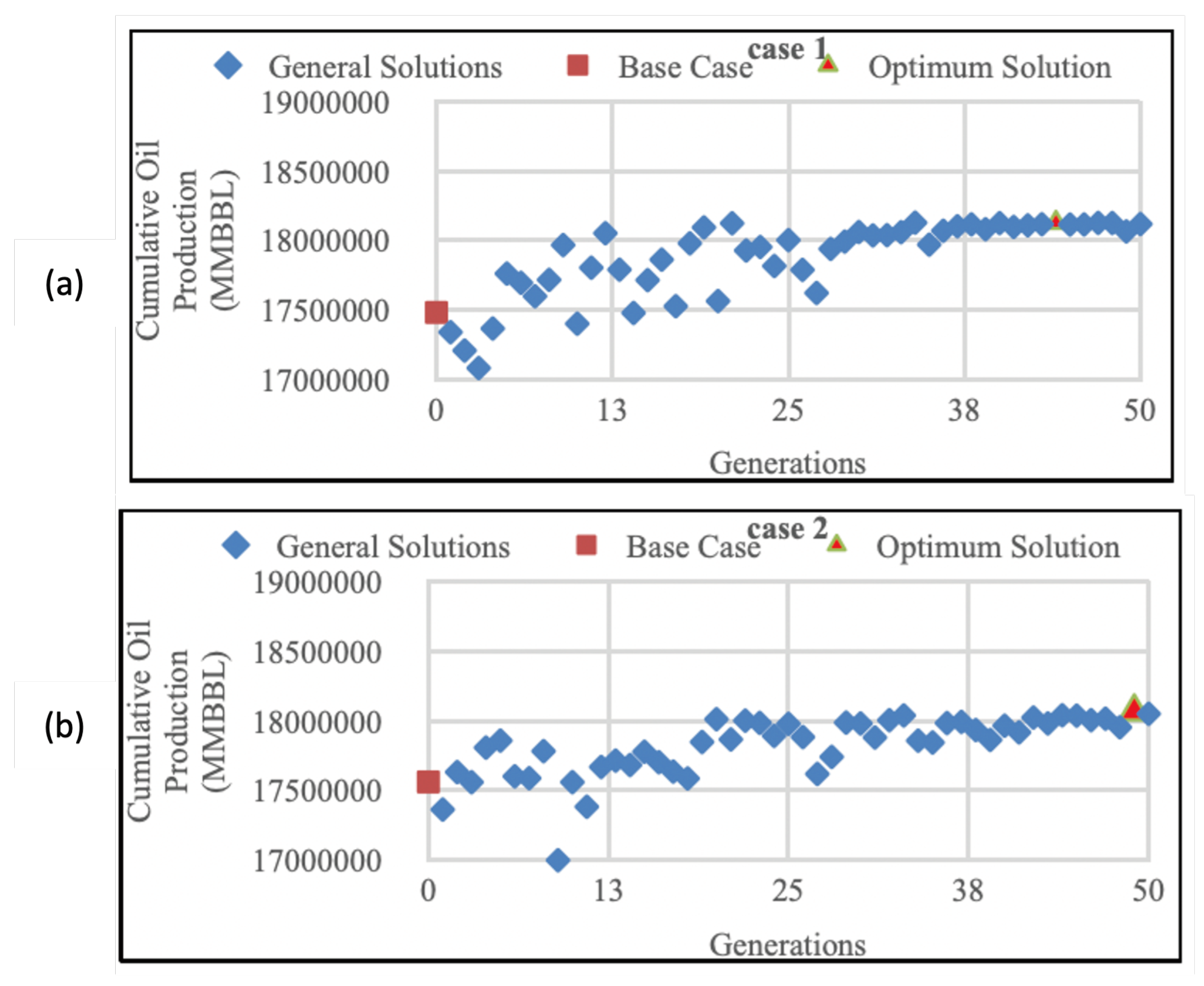
From the result obtained in Figure 2a, the base case cumulative oil production for Case 1 was 17484 MBBL, and it reached its optimum solution at the 44th generation with 18130 MBBL of cumulative oil production. The cumulative oil production has increased by 3.6% compared to the initial cumulative oil production before optimization. Figure 2b shows that Case 2 initially had 17562 MBBL of cumulative oil production, which increased by 2.88% to the optimum value of 18068 MBBL at the 49th generation.
However, the difference between the optimized value of Case 1 and 2 was only 0.81%. This indicates that the different initial well placement distribution did not have a significant impact on GA performance and the cumulative oil produced over 50 generations. The assumption for this result was because of GA’s stochastic nature of randomly searching for random solutions and hence initial well placement distribution did not significantly have an impact on the cumulative oil produced.
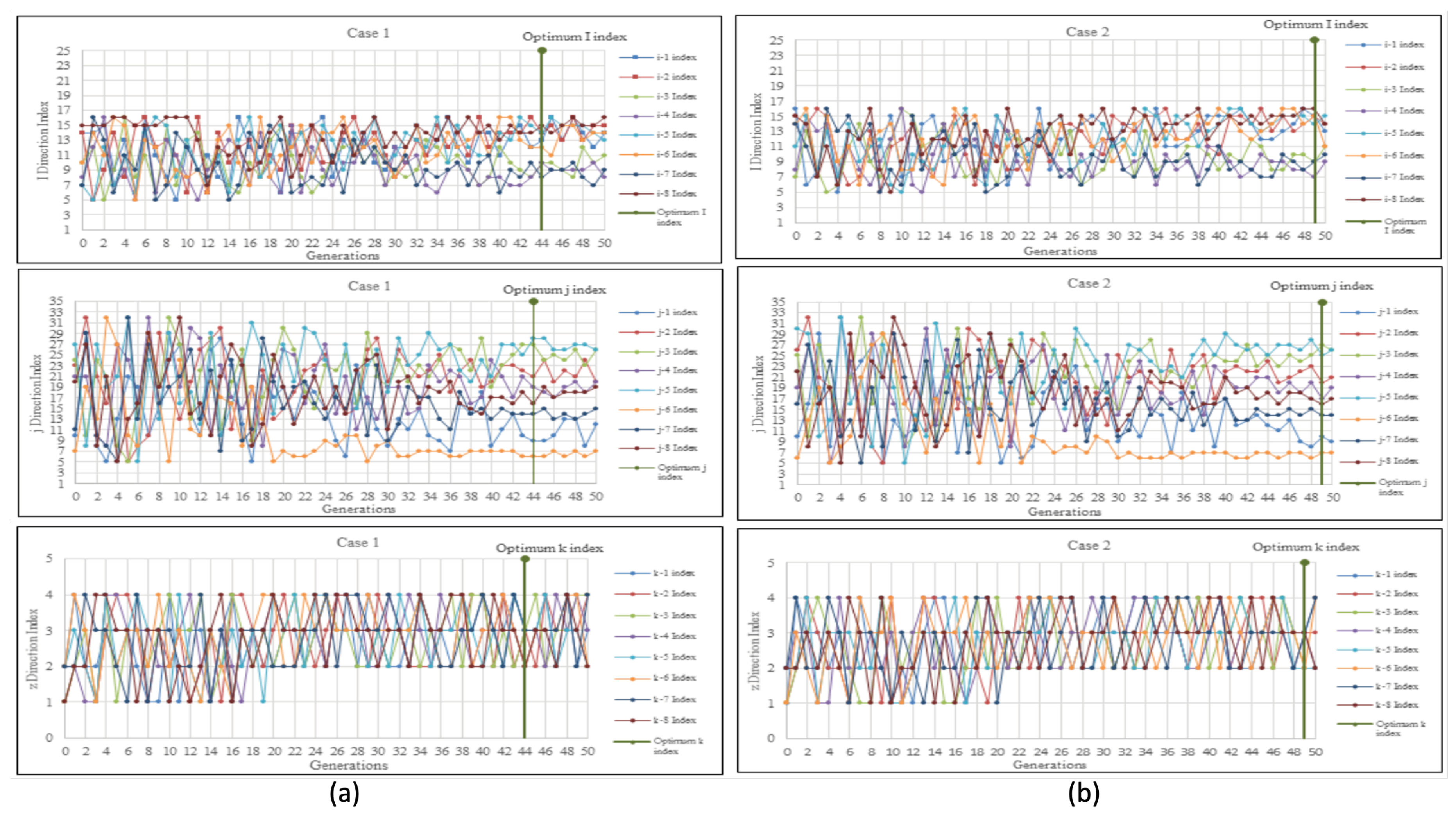
In Case 1, Figure 3a (i) illustrates the optimization of the i-direction index for all 8 producers. The range of index values considered for optimization was between 5 and 16, in order to reduce the number of cells that needed evaluation. Initially, the i-direction indexes were dispersed randomly across the first 10 generations, ranging from a minimum of 5 indexes to a maximum of 16 indexes. However, as the generations progressed, these values gradually decreased. By the 40th generation, a more consistent pattern emerged, with the optimum i-direction indexes observed at the 44th generation, coinciding with the peak cumulative oil production.
In Figure 3a (j), the optimization of the j-direction index for all 8 producers is depicted. Similarly, the index values for the j-direction were optimized within the range of 5 to 32, in order to limit the number of cells to be evaluated. In the initial 20 generations, the j-direction indexes were scattered randomly, with a minimum of 5 indexes and a maximum of 32 indexes involved. Gradually, the intervals of decrease became smaller as the generations progressed, peaking at the 50th generation. From the 42nd generation onward, there was a noticeable trend in the graph pattern, with the j indexes displaying greater consistency. The optimal j indexes were observed at the 44th generation, coinciding with the achievement of the optimal cumulative oil production.
In Figure 3a (k), the optimization of the k-direction index for all 8 producers in Case 1 is depicted. Since the synthetic reservoir model consisted of only 4 layers, the k-direction indexes for the 8 producers were optimized within the range of indexes 1 to 4. Initially, in the first 20 generations, the graph showed a random scattering of k indexes, with a minimum of 1 and a maximum of 4 k-direction indexes. However, starting from the 20th generation, the graph pattern indicated a growing consistency in the k indexes. The optimal k indexes were achieved at the 44th generation, aligning with the attainment of the optimal cumulative oil production.
In Case 2, Figure 3b (i) illustrates the optimization of the i-direction index for all 8 producers. The range of optimization falls between index 5 and 16, effectively reducing the number of cells to be evaluated. Initially, the i-direction indexes were scattered randomly in the first 10 generations, ranging from a minimum of 5 to a maximum of 16. However, as the generations progressed up to a maximum of 50, these indexes gradually decreased at intervals. Notably, by the 40th generation, the graph pattern indicated a greater consistency in the I indexes, with the optimal indexes observed at the 49th generation coinciding with the optimal cumulative oil production.
Similarly, Figure 3b (j) demonstrates the optimization of the j-direction index for all 8 producers in Case 2. The optimization range for the j-direction indexes spans from index 5 to 32, effectively limiting the number of cells to be evaluated. In the initial 20 generations, the j-direction indexes were scattered randomly, ranging from a minimum of 5 to a maximum of 32.
The generations saw a gradual decrease in intervals, with a maximum of 50 generations. At the 40th generation, the graph displayed a more consistent pattern for the j indexes, reaching optimal values at the 49th generation when the cumulative oil production was at its peak.
In Figure 3b (k), the optimization of the k-direction index for all 8 producers is depicted for Case 2. As the synthetic reservoir model consisted of only 4 layers, the k-direction indexes for the 8 producers were optimized within the range of 1 to 4. Initially, the graph showed a random scattering of k indexes for the first 20 generations, ranging from a minimum of 1 to a maximum of 4. However, starting from the 21st generation, the k indexes became more consistent, reaching their optimal values at the 49th generation when the cumulative oil production was at its peak.
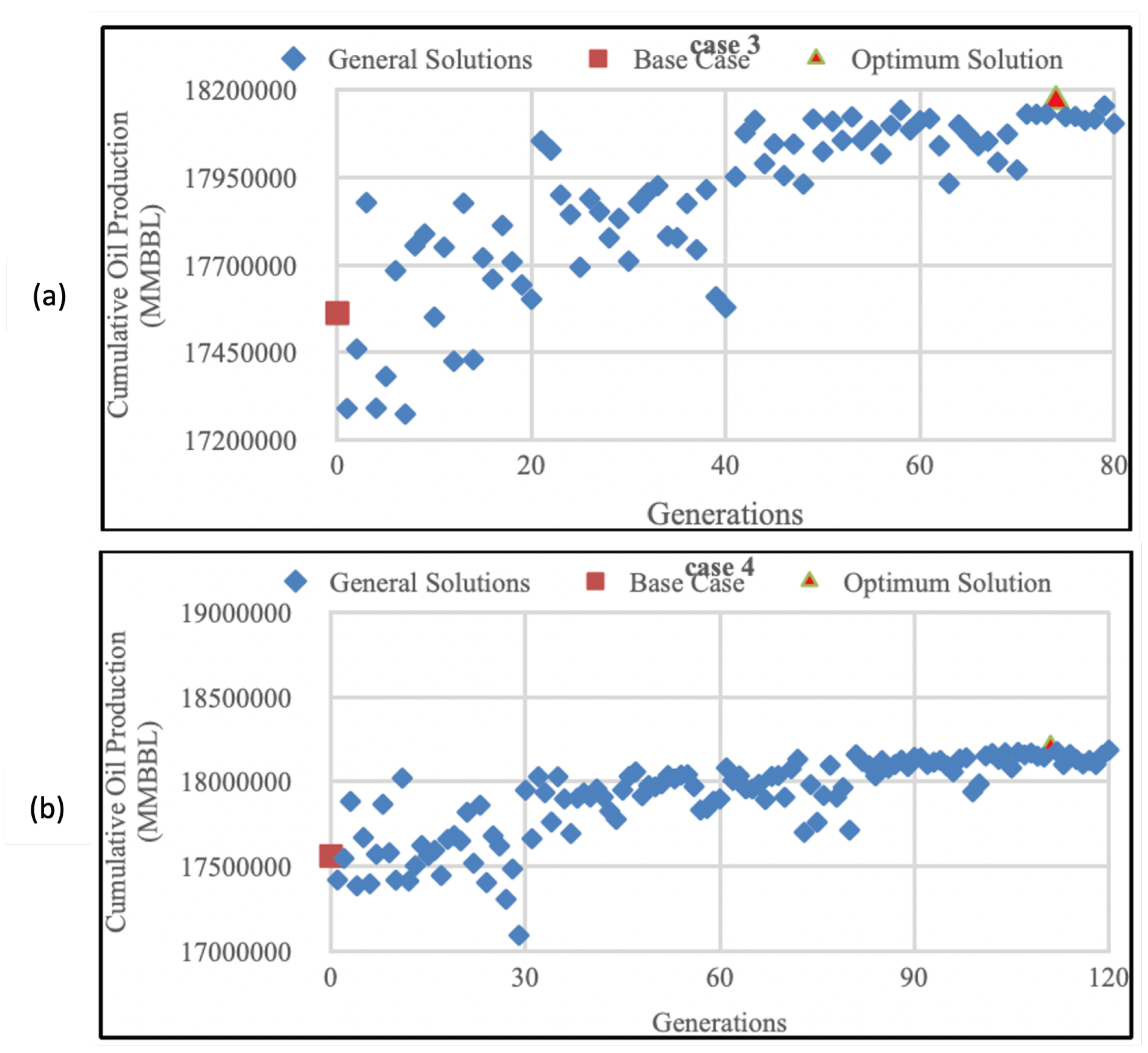
In Figure 4a, it was observed that Case 3 achieved the optimal solution after 74 generations, resulting in a cumulative oil production of 18169 MBBL. This represents a 3.46% increase compared to the initial cumulative oil production before optimization.
Moving on to Case 4, Figure 4b illustrated that the cumulative oil production increased by 3.63% to reach a value of 18200 MBBL at the optimum point. This was achieved after 111 generations. Comparing Case 4 to Case 3, there was a slight improvement of 0.17
These findings suggest that increasing the number of potential well placement solutions leads to a greater genetic richness, which in turn increases the likelihood of converging towards the optimal cumulative oil production. However, it is important to note that a larger number of random solutions requires more iterations or generations, as seen in Cases 3 and 4. Specifically, Case 3 reached the optimum solution in just 74 generations, while Case 4 required 111 generations. In conclusion, employing a larger number of random solutions enhances the probability of reaching the optimal solution, albeit at the cost of additional generations. The optimized well placements for Cases 3 and 4 can be observed in Figure 4a,b, respectively.
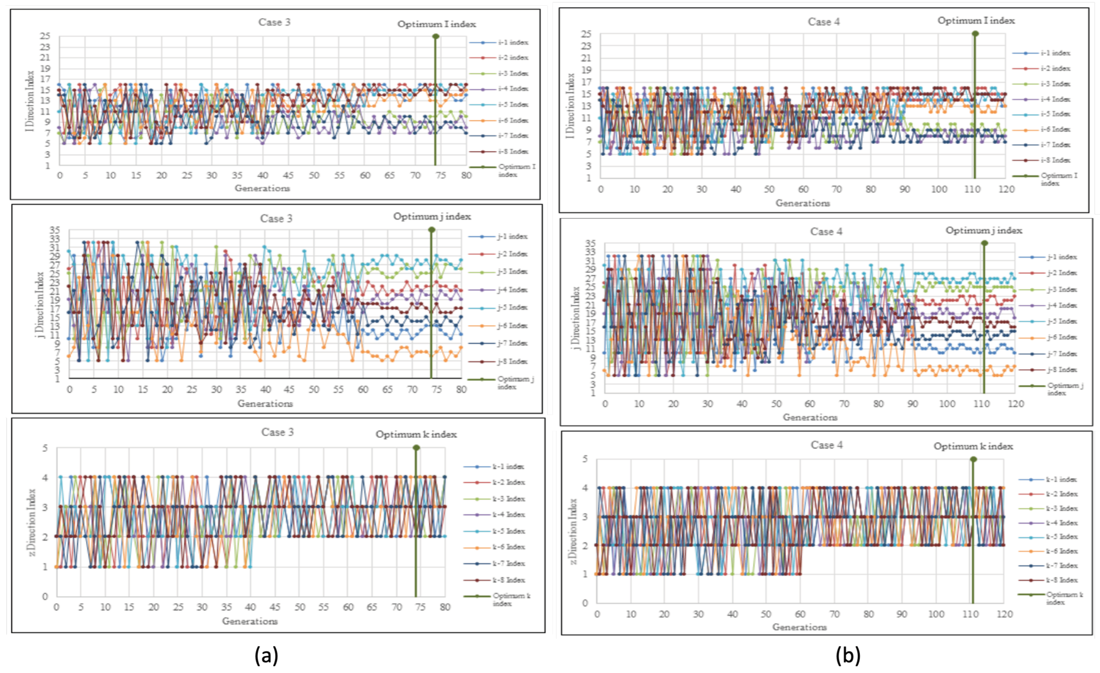
For Case 3, the optimisation of each of the eight manufacturers’ i-direction index is displayed in Figure 5a (i). To reduce the number of cells that need to be assessed, all eight producers’ i-direction indexes were optimised in the range between index 5 and index 16. The graph demonstrated how, over the first 22 generations, the direction I indices were dispersed at random, with a minimum of 5 and a maximum of 16 i-direction index. Even yet, they steadily dropped off as the generations increased to a maximum of 80. The graph pattern demonstrated that the I indexes started to become more consistent at generation 55. As the optimum cumulative oil production achieved an optimal solution, generation 74 saw the observation of the optimum I indexes.
The optimisation of the j-direction index for Case 3 across all 8 producers is displayed in Figure 5a (j). To reduce the number of cells to be assessed, all eight manufacturers’ j-direction indexes were optimised between index 5 and index 32. With a minimum of 5 and a maximum of 32 j-direction indices involved, the graph demonstrated how the direction j indexes were randomly dispersing throughout the first 20 generations. Even Nevertheless, when the generations increased to a maximum of 80, they progressively reduced at intervals. The j indexes started to become more consistent at the 60th generation, according to the graph pattern, and the optimum j indexes were found to be at the 74th generation when the optimum cumulative oil production achieved an optimal solution.
The optimisation of each of the eight producers’ k-direction index for Case 3 is displayed in Figure 5a (k). Since the artificial reservoir model was limited to four layers, all k-direction indices for eight producers were optimised in the range between indexes 1 and 4. The graph demonstrated how, over the first 40 generations, the direction k indices were randomly dispersed, with a minimum of 1 k-direction index and a maximum of 4 k-direction indexes. The graph pattern indicated that the k indexes started to become consistent at generation 41, and the optimum k indexes were found to be at generation 74 when the optimum cumulative oil production achieved an optimal solution.
Figure 5b (i) shows the optimization of the i-direction index of all 8 producers for Case 4. All i-direction indexes for 8 producers were optimized in the interval between index 5 to 16 to limit the number of cells to be evaluated. The graph showed the direction I indexes were scattered randomly in the first 50 generations with a minimum of 5 i-direction index and a maximum of 16 i-direction index. Still, they gradually decreased in intervals as the generations reached a maximum generation of 120. Starting at the 80th generation, the graph pattern showed that the I indexes began to be more consistent and the optimum I indexes were observed to be at the 111th generation as the optimum cumulative oil production reached an optimal solution.
Figure 5b (j) shows the optimization of the j-direction index of all 8 producers for Case 4. All j-direction indexes for 8 producers were optimized in the interval of between index 5 to 32 to limit the number of cells to be evaluated. The graph showed the direction j indexes were scattering randomly in the first 30 generations with a minimum of 5 j-direction index and a maximum of 32 j-direction index. Still, they gradually decreased in intervals as the generations reached a maximum generation of 120. Starting at the 90th generation, the graph pattern showed that the j indexes began to be more consistent and the optimum j indexes were observed to be at the 111th generation as the optimum cumulative oil production reached an optimal solution.
Figure 5b (k) shows the optimization of the k-direction index of all 8 producers for Case 4. All k-direction indexes for 8 producers were optimized in the interval between indexes 1 to 4 because the synthetic reservoir model was only a 4-layered model. The graph showed the direction k indexes were scattering randomly in the first 60 generations with a minimum of 1 k-direction index and a maximum of 4 k-direction index. Starting at the 61st generation, the graph pattern showed that the k indexes began to be consistent and the optimum k indexes were observed to be at the 111th generation as the optimum cumulative oil production reached an optimal solution.
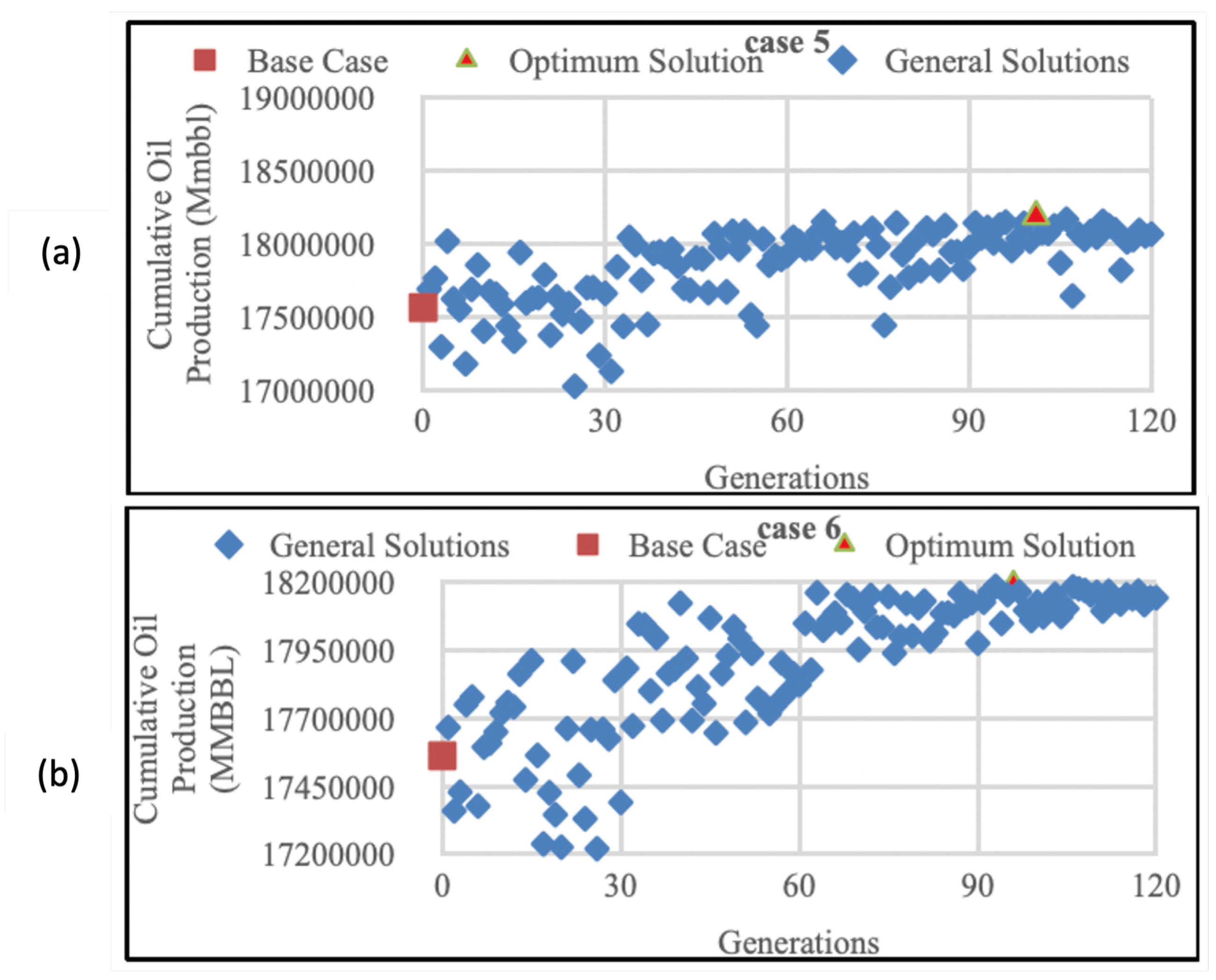
From the result obtained in Figure 6a, Case 5 reached the optimum solution at the 101st generation with 18189 MBBL of cumulative oil production. The cumulative oil production has increased by 3.57% compared to the initial cumulative oil production before optimization. For Case 6, cumulative oil production increased also by 3.57% at an optimum value of 18188 MBBL with 96 generations, as shown in Figure 6b.
The findings demonstrated that, despite using various crossover rates, Cases 5 and 6 did not differ significantly in terms of the total amount of oil produced. According to theory, a higher crossover rate causes generations or iterations to continue, increasing the likelihood that they will converge to global optima. Even still, Case 6’s 0.9 crossover rate resulted in less cumulative oil production than Case 4’s 0.8 crossover rate. Figure 6a,b display the optimised well placement that was achieved for Cases 5 and 6.
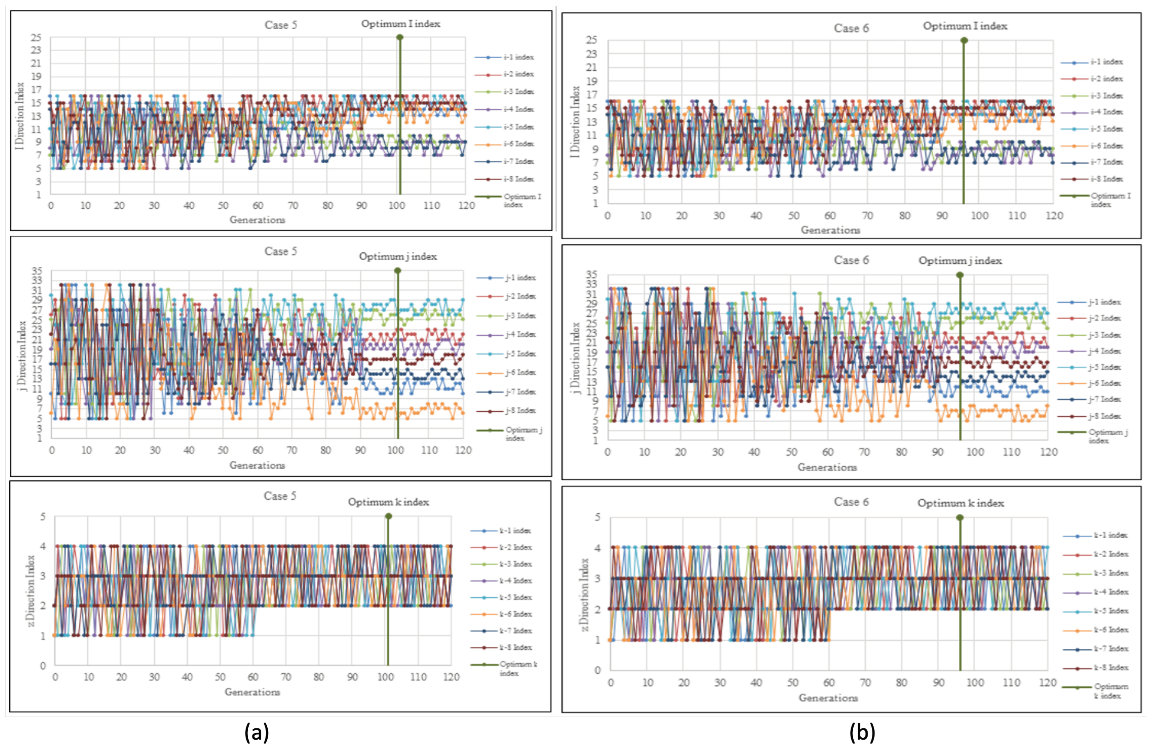
Figure 7a (i) shows the optimization of the i-direction index of all 8 producers for Case 5. All i-direction indexes for 8 producers were optimized in the interval between index 5 and 16 to limit the number of cells to be evaluated. The graph showed the direction I indexes were scattered randomly in the first 40 generations with a minimum of 5 i-direction index and a maximum of 16 i-direction index. Still, they gradually decreased in intervals as the generations reached a maximum generation of 120. Starting at the 90th generation, the graph pattern showed that the I indexes began to be more consistent, and the optimum I indexes were observed to be at the 101st generation as the optimum cumulative oil production reached an optimal solution.
Figure 7a (j) shows the optimization of the j-direction index of all 8 producers for Case 5. All j-direction indexes for 8 producers were optimized in the interval between index 5 and 32 to limit the number of cells to be evaluated. The graph showed the direction j indexes were scattering randomly in the first 30 generations, with a minimum of 5 j-direction index and a maximum of 32 j-direction index. Still, they gradually decreased in intervals as the generations reached a maximum generation of 120. Starting at the 90th generation, the graph pattern showed that the j indexes began to be more consistent, and the optimum j indexes were observed to be at the 101st generation as the optimum cumulative oil production reached an optimal solution.
Table 1. Case Comparative Analysis for Cumulative Oil Production.
Cumulative Oil Production
Cases Base, (MBBL) Optimum, (MBBL) Production Increment Case Change
Case 1
4th generations
17484 18130 3.69 % 0.81%
Case 2
49th generations
17562 18068 2.88 %
Case 3
74th generations
17561 18169 3.46 % 0.17%
Case 4
111st generations
17562 18200 3.63 %
Case 5
101st generations
17562 18189 3.57 % 0%
Case 6
96th generations
17561 18188 3.57 %
Figure 7a (k) shows the optimization of the k-direction index of all 8 producers Case 5. All k-direction indexes for 8 producers were optimized in the interval between indexes 1 and 4 because the synthetic reservoir model was only a 4-layered model. The graph showed the direction k indexes were scattering randomly in the first 60 generations, with a minimum of 1 k-direction index and a maximum of 4 k-direction index involved. Starting at the 61st generation, the graph pattern showed that the k indexes began to be consistent, and the optimum k indexes were observed to be at the 101st generation as the optimum cumulative oil production reached an optimal solution.
Figure 7b (i) shows the optimization of the i-direction index of all 8 producers for Case 6. All i-direction indexes for 8 producers were optimized in the interval between index 5 to 16 to limit the number of cells to be evaluated. The graph showed the direction I indexes were scattered randomly in the first 50 generations, with a minimum of 5 i-direction index and a maximum of 16 i-direction index. Still, they gradually decreased in the interval as the generations reached a maximum generation of 120. Starting at the 90th generation, the graph pattern showed that the I indexes began to be more consistent, and the optimum I indexes were observed to be at the 96th generation as the optimum cumulative oil production reached an optimal solution.
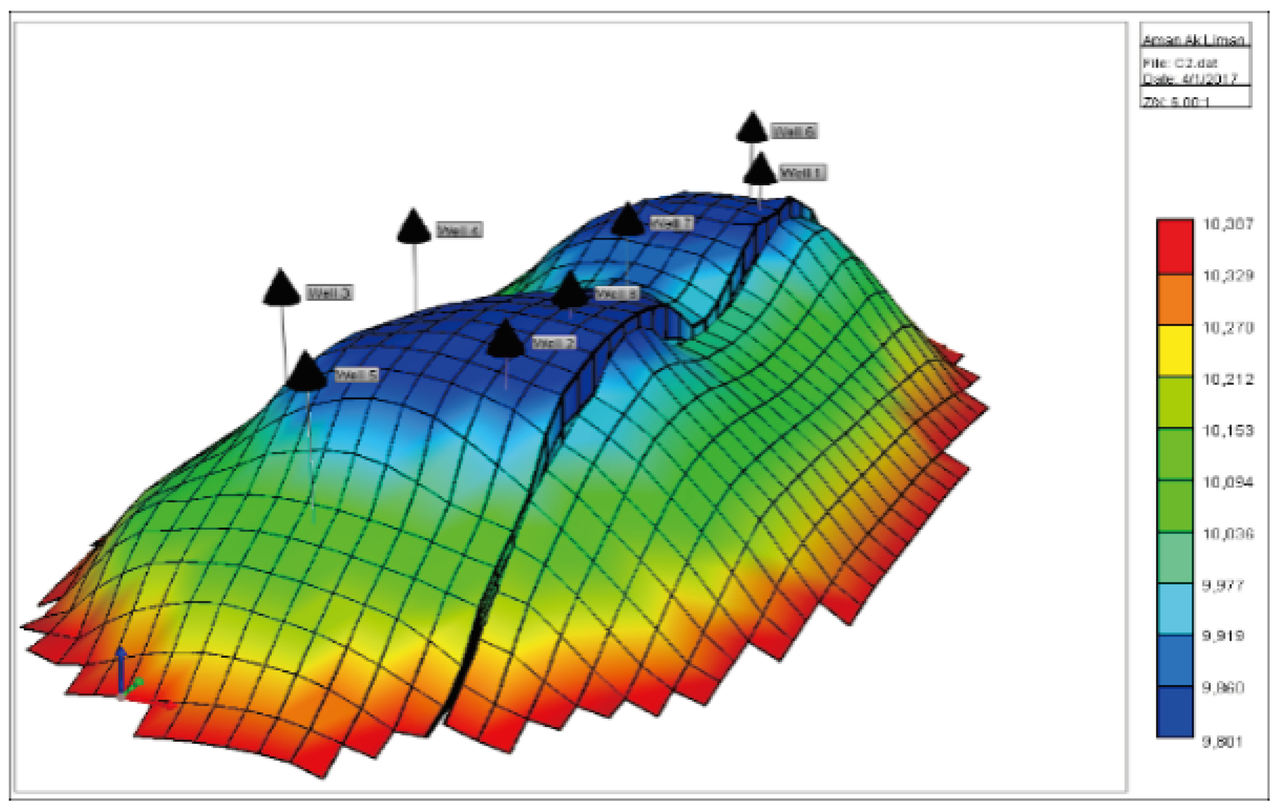
Figure 7b (j) shows the optimization of the j-direction index of all 8 producers for Case 6. All j-direction indexes for 8 producers were optimized in the interval between index 5 and 32 to limit the number of cells to be evaluated. The graph showed the direction j indexes were scattering randomly in the first 30 generations, with a minimum of 5 j-direction index and a maximum of 32 j-direction index. Still, they gradually decreased in intervals as the generations reached a maximum generation of 120. Starting at the 90th generation, the graph pattern showed that the j indexes began to be more consistent, and the optimum j indexes were observed to be at the 96th generation as the optimum cumulative oil production reached an optimal solution.
Figure 7b (k) shows the optimization of the k-direction index of all 8 producers for Case 6. All k-direction indexes for 8 producers were optimized in the interval between indexes 1 and 4 because the synthetic reservoir model was only a 4-layered model. The graph showed the direction k indexes were scattering randomly in the first 60 generations, with a minimum of 1 k-direction index and a maximum of 4 k-direction index involved. Starting at the 61st generation, the graph pattern showed that the k indexes began to be consistent, and the optimum k indexes were observed to be at the 96th generation as the optimum cumulative oil production reached an optimal solution.

4. Conclusions

GA was still able to optimize the cumulative oil production to an optimum solution even though different initial well placement distributions were used. The assumption made for this result was because of the stochastic nature of genetic algorithms, it randomly searched for random solutions instead of guessing on the initial solutions, and hence the cumulative oil produced will still be optimized with no dependency on the initial well placement distribution.
A higher number of random solutions was used, resulting in higher cumulative oil production. A greater number of possible well placement solutions used induced a greater number of potential solutions (genetic richness), which eventually led to a higher probability of convergence towards optimum cumulative oil production. However, a larger number of random solutions required more iteration or generation, as observed in Cases 3 and 4. It can be concluded that a larger number of random solutions used increases the probability of reaching the optimum solution, but it will take more generations. A higher crossover rate improved the homogenization of the population. However, a larger number of random solutions size is needed to see a more significant effect of the crossover rate on the cumulative oil production.
The genetic algorithm optimization engine in CMOST demonstrated a powerful search methodology that is recommended to be applied in complex oil fields. Genetic algorithms overcome the limitations and deliver the desired optimum objective function compared to traditional methods that are limited by the non-linearity and non-continuity of the reservoir’s geological behaviour. The optimization methodology in this project is recommended to be modified by combining it with other accelerating algorithms such as artificial neural networks, hill climbing, and upscaling to reduce its computing time and increase stability.

Author Contributions

F“Conceptualization, S.I.; methodology, S.I; validation, A.S., S.I.; formal analysis, S.I., and D.D.K.W.; investigation, S.I., and D.D.K.W.; resources, A.S., J.K., and S.I.; data curation, S.I., and D.D.K.W.; writing—original draft preparation, S.I; writing—review and editing, S.I., and D.D.K.W. visualization, S.I., and D.D.K.W.; supervision, S.I., A.S., and J.K.; project administration, A.S., J.K., and S.I.; funding acquisition, A.S., J.K., and S.I. All authors have read and agreed to the published version of the manuscript.

Funding

This research was funded by Nazarbayev University grant numbers 11022021CRP1512 and 08042FD1911, and the APC was funded by 11022021CRP1512.

Acknowledgments

Any opinions, findings, conclusions, or recommendations expressed in this material are those of the author(s) and do not necessarily reflect the views of Nazarbayev University.

Conflicts of Interest

The authors hereby declare that the research presented in this paper was not impacted by any known conflicting financial interests or personal connections.

Abbreviations

The following abbreviations are used in this manuscript:
CMG Computer Modeling Group
GA Genetic Algorithm
BBL Barrel

References

  1. Aanonsen, S. I., Eide, A. L., Holden, L., and J. O. Aasen. Optimizing Reservoir Performance Under Uncertainty with Application to Well Location. In Proceedings of the SPE Annual Technical Conference and Exhibition, Dallas, Texas, USA, October 1995; SPE-30710-MS. [CrossRef]
  2. Beckner, B. L., and X. Song. Field Development Planning Using Simulated Annealing - Optimal Economic Well Scheduling and Placement. In Proceedings of the SPE Annual Technical Conference and Exhibition, Dallas, Texas, USA, October 1995; SPE-30650-MS. [CrossRef]
  3. Bittencourt, Antonio C., and Roland N. Horne. Reservoir Development and Design Optimization. In Proceedings of the SPE Annual Technical Conference and Exhibition, San Antonio, Texas, USA, 97; SPE-38895-MS. [CrossRef]
  4. Grefenstette J.J. Genetic Algorithms for Machine Learning, 1st ed.; Publisher: Springer New York, NY, USA, 1994; pp. IV, 165. [CrossRef]
  5. Guyaguler, B., Horne, R. N., Rogers, L., and Jacob J. R. Optimization of Well Placement in a Gulf of Mexico Waterflooding Project. SPE Res Eval & Eng 2002, 5, 229–236. [CrossRef]
  6. John H., H. Adaptation in natural and artificial systems: an introductory analysis with applications to biology, control, and artificial intelligence, 1st ed.; MIT Press: USA, 1992; p. 211. Available online: https://ieeexplore.ieee.org/servlet/opac?bknumber=6267401.
  7. Montes, G., Bartolome, Pablo, and Angel L. Udias. The Use of Genetic Algorithms in Well Placement Optimization. In Proceedings of the SPE Latin American and Caribbean Petroleum Engineering Conference, Buenos Aires, Argentina, March 2001; SPE-69439-MS. [CrossRef]
  8. Pan, Y., and Roland N. H. Improved Methods for Multivariate Optimization of Field Development Scheduling and Well Placement Design. In Proceedings of the SPE Annual Technical Conference and Exhibition, New Orleans, Louisiana, September 1998; SPE-49055-MS. [CrossRef]
  9. Santellani, G., Hansen, B., and T. Herring. Survival of the Fittest: "An Optimized Well Location Algorithm for Reservoir Simulation". In Proceedings of the SPE Asia Pacific Conference on Integrated Modeling for Asset Management, Kuala Lumpur, Malaysia, March 1998; SPE-39754-MS. [CrossRef]
  10. Seifert, D., Lewis, J.J.M., Hern, C.Y., and N.C.T. Steel. Well Placement Optimisation and Risking using 3-D Stochastic Reservoir Modelling Techniques. In Proceedings of the European 3-D Reservoir Modelling Conference, Stavanger, Norway, April 1996; SPE-35520-MS. [CrossRef]
  11. Yeten, B., Durlofsky, L. J., and Khalid A. OOptimization of Nonconventional Well Type, Location, and Trajectory. SPE J. 2003, 8, 200–210. [CrossRef]
Figure 1. 3D view grid top of synthetic model.
Preprints 100127 g001
Figure 2. Optimization for different initial well placement distribution (a) Case 1 (b) Case 2.
Preprints 100127 g002
Figure 3. i-j index optimization (a) case 1 (b) Case 2.
Preprints 100127 g003
Figure 4. Optimization for different random solutions size (a) Case 3 (b) Case 4.
Preprints 100127 g004
Figure 5. i-j index optimization (a) case 3 (b) Case 4.
Preprints 100127 g005
Figure 6. Optimization for different random solutions size (a) Case 5 (b) Case 6.
Preprints 100127 g006
Figure 7. i-j index optimizations (a) case 5 (b) Case 6.
Preprints 100127 g007
Disclaimer/Publisher’s Note: The statements, opinions and data contained in all publications are solely those of the individual author(s) and contributor(s) and not of MDPI and/or the editor(s). MDPI and/or the editor(s) disclaim responsibility for any injury to people or property resulting from any ideas, methods, instructions or products referred to in the content.
Copyright: This open access article is published under a Creative Commons CC BY 4.0 license, which permit the free download, distribution, and reuse, provided that the author and preprint are cited in any reuse.
Prerpints.org logo

Preprints.org is a free preprint server supported by MDPI in Basel, Switzerland.

Subscribe

© 2024 MDPI (Basel, Switzerland) unless otherwise stated