Submitted:
03 March 2024
Posted:
05 March 2024
You are already at the latest version
Abstract
Keywords:
1. Introduction
2. Material and Methods
2.1. Study Area
2.2. Data
2.2.1. Landsat and Sentinel-1/2 Data and Pre-Processing
2.2.2. Land Cover Data
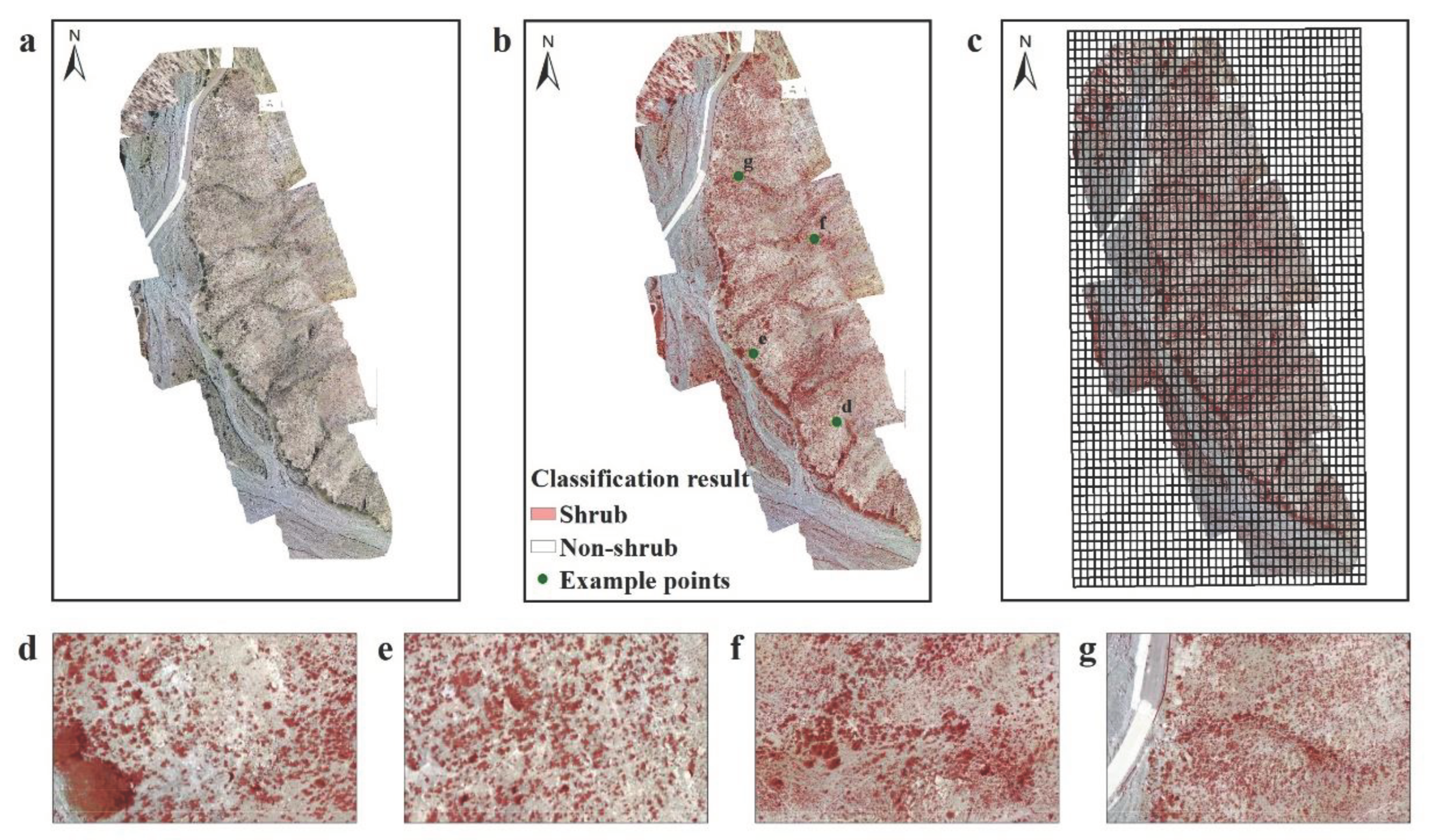
2.2.3. Ground-based Measurements and UAV Field Images
2.2.4. Auxiliary Datasets
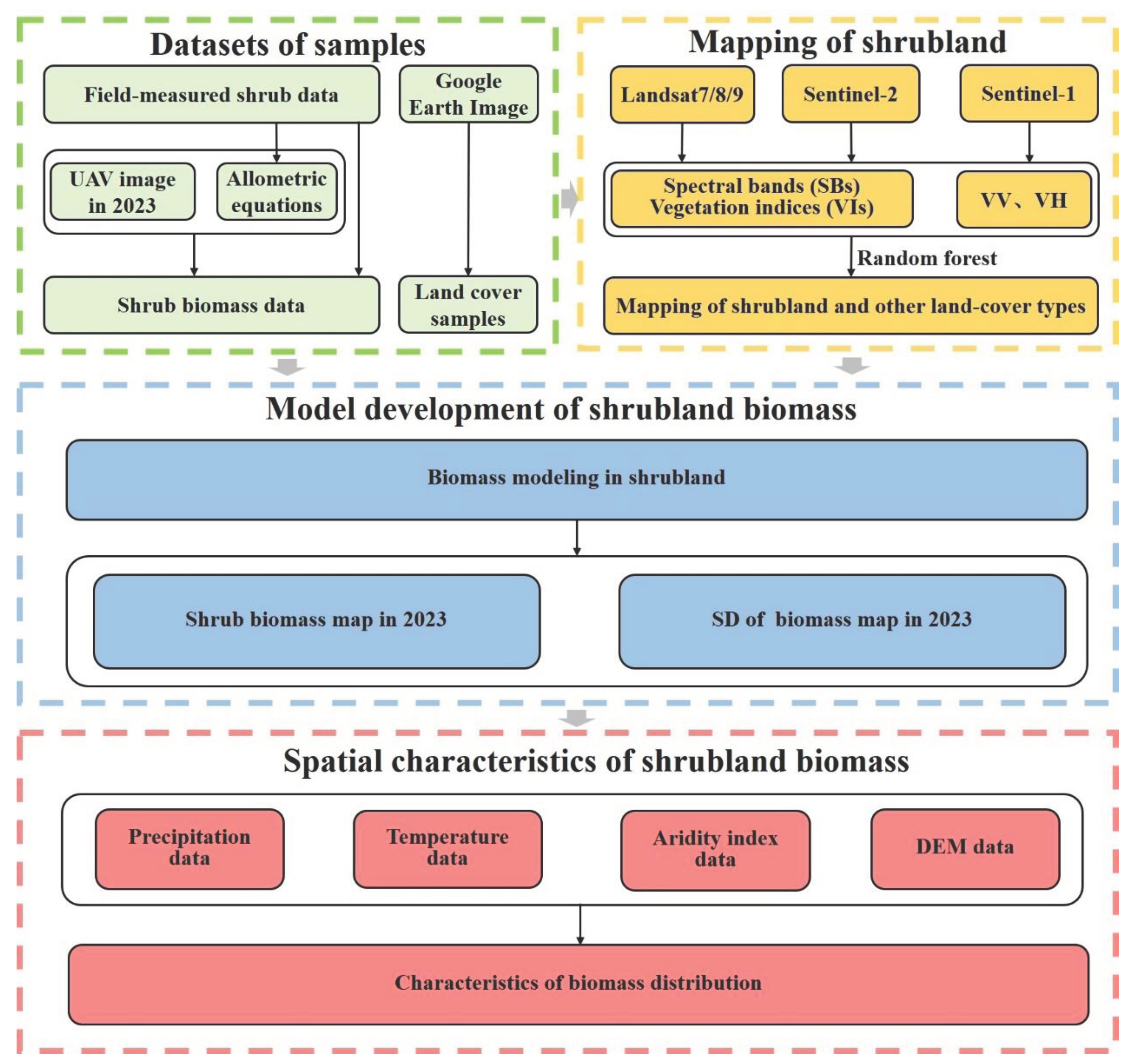
2.3. Method
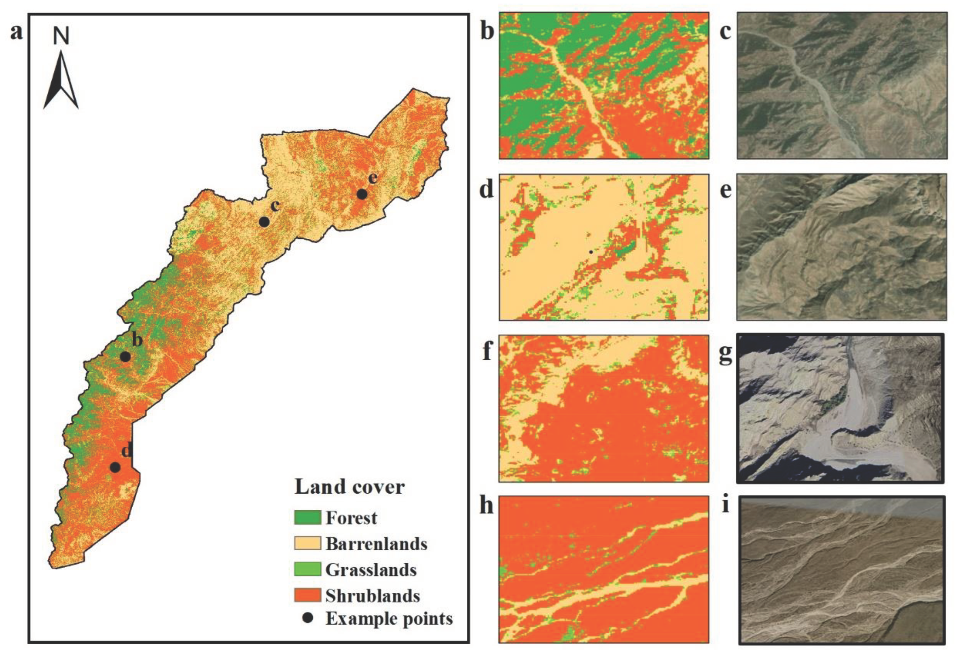
2.3.1. Mapping of Shrubland and Other Land Cover Types
2.3.2. Calculation of Biomass at the Shrub Level
2.3.3. Calculation of Biomass at the UAV Plot Level
2.3.4. Satellite-based Modeling of Shrubland Biomass at the Regional Level
2.3.5. Regional Implementation of the Satellited-based Shrubland Biomass Model
2.3.6. Characteristics of the Shrubland Biomass
3. Results
3.1. Mapping of Shrubland and Other Land-Cover Types
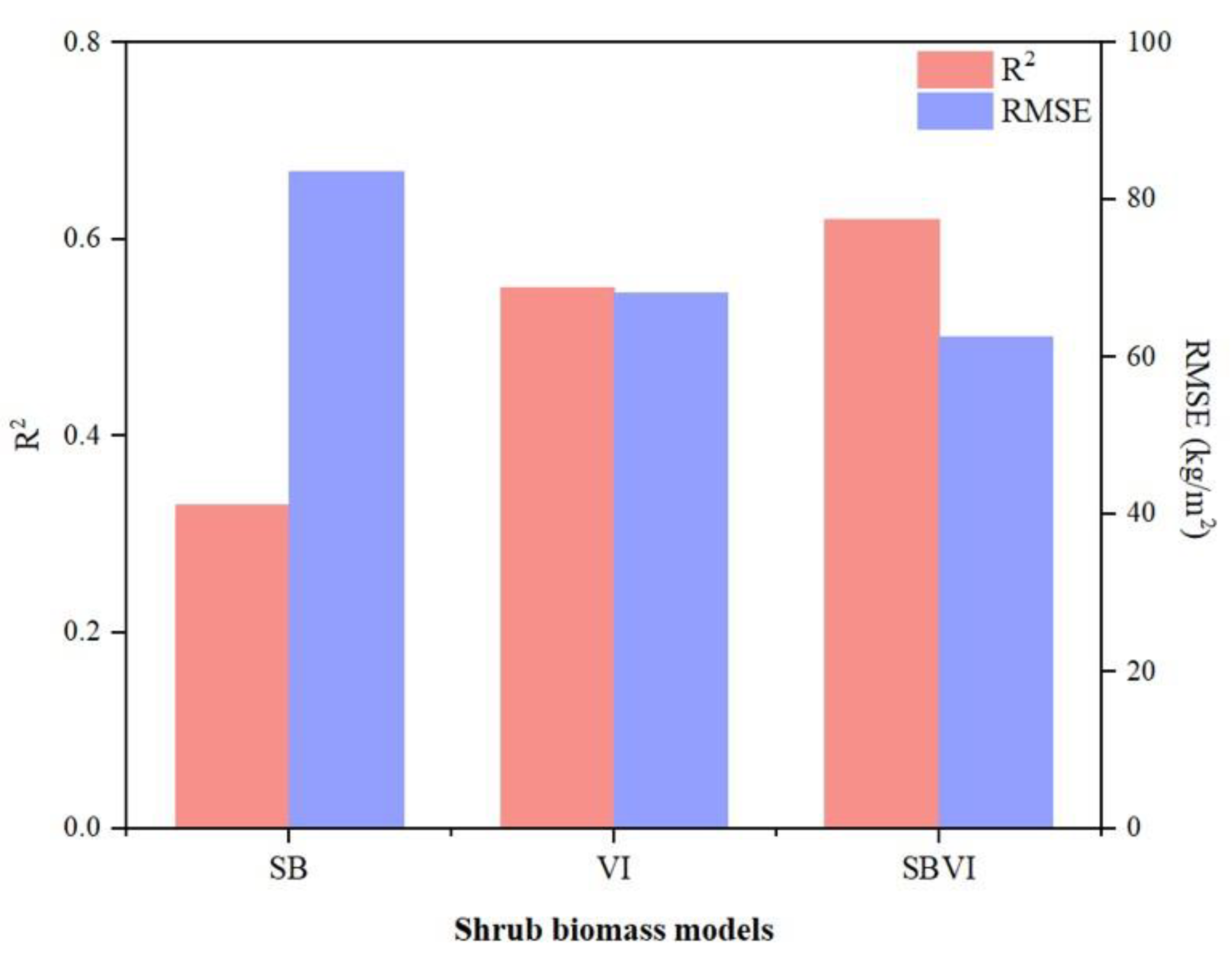
3.2. Selection of the Best Model and Variable Importance Analysis
3.3. Biomass Mapping in the Shrubland
3.4. Distribution of Shrub Biomass under Different Factors
4. Discussion
4.1. Algorithms
4.2. Spatial Characteristics of Biomass in Shrubland
5. Conclusions
Funding
References
- Vezzoni, R.; Sijtsma, F.; Vihinen, H. Designing Effective Environmental Policy Mixes in the UN Decade on Ecosystem Restoration. Ecosyst. Serv. 2023, 62, 101541. [CrossRef]
- Zhao, Y.; Wang, J.; Zhang, G.; Liu, L.; Yang, J.; Wu, X.; Biradar, C.; Dong, J.; Xiao, X. Divergent Trends in Grassland Degradation and Desertification under Land Use and Climate Change in Central Asia from 2000 to 2020. Ecol. Indic. 2023, 154, 110737. [CrossRef]
- Trenberth, K.E. Climate Change Caused by Human Activities Is Happening and It Already Has Major Consequences. J. Energy Nat. Resour. Law 2018, 36, 463–481. [CrossRef]
- Xiong, Y.; Mo, S.; Wu, H.; Qu, X.; Liu, Y.; Zhou, L. Influence of Human Activities and Climate Change on Wetland Landscape Pattern—A Review. Sci. Total Environ. 2023, 879, 163112. [CrossRef]
- Parmenter, R.R.; MacMahon, J.A. Factors Determining the Abundance and Distribution of Rodents in a Shrub-Steppe Ecosystem: The Role of Shrubs. Oecologia 1983, 59, 145–156. [CrossRef]
- Jankju, M. Role of Nurse Shrubs in Restoration of an Arid Rangeland: Effects of Microclimate on Grass Establishment. J. Arid Environ. 2013, 89, 103–109. [CrossRef]
- Ballantyne, M.; Pickering, C.M. Shrub Facilitation Is an Important Driver of Alpine Plant Community Diversity and Functional Composition. Biodivers. Conserv. 2015, 24, 1859–1875. [CrossRef]
- Li, J.; Zhao, C.Y.; Song, Y.J.; Sheng, Y.; Zhu, H. Spatial Patterns of Desert Annuals in Relation to Shrub Effects on Soil Moisture. J. Veg. Sci. 2010, 21, 221–232. [CrossRef]
- Garcia-Estringana, P.; Alonso-Blázquez, N.; Marques, M.J.; Bienes, R.; González-Andrés, F.; Alegre, J. Use of Mediterranean Legume Shrubs to Control Soil Erosion and Runoff in Central Spain. A Large-Plot Assessment under Natural Rainfall Conducted during the Stages of Shrub Establishment and Subsequent Colonisation. CATENA 2013, 102, 3–12. [CrossRef]
- Boelman, N.T.; Gough, L.; Wingfield, J.; Goetz, S.; Asmus, A.; Chmura, H.E.; Krause, J.S.; Perez, J.H.; Sweet, S.K.; Guay, K.C. Greater Shrub Dominance Alters Breeding Habitat and Food Resources for Migratory Songbirds in Alaskan Arctic Tundra. Glob. Change Biol. 2015, 21, 1508–1520. [CrossRef]
- Wilczek, A.; Jura, J.; Włoch, W.; Kojs, P.; Szendera, W. The Significance of the Field Shrubs and Hedges in Biodiversity Conservation : The Old Field Shrubs and Hedges of Silesian Biotanical Garden. Czyżnie i ich znaczenie w ochronie różnorodności biologicznej. Stare czyżnie w Śląskim Ogrodzie Botanicznym 2005.
- Návar, J.; Méndez, E.; Nájera, A.; Graciano, J.; Dale, V.; Parresol, B. Biomass Equations for Shrub Species of Tamaulipan Thornscrub of North-Eastern Mexico. J. Arid Environ. 2004, 59, 657–674. [CrossRef]
- Chai, Y.; Zhong, J.; Zhao, J.; Guo, J.; Yue, M.; Guo, Y.; Wang, M.; Wan, P. Environment and Plant Traits Explain Shrub Biomass Allocation and Species Composition across Ecoregions in North China. J. Veg. Sci. 2021, 32, e13080. [CrossRef]
- Gómez-Aparicio, L.; Zamora, R.; Gómez, J.M.; Hódar, J.A.; Castro, J.; Baraza, E. Applying Plant Facilitation to Forest Restoration: A Meta-Analysis of the Use of Shrubs as Nurse Plants. Ecol. Appl. 2004, 14, 1128–1138. [CrossRef]
- Yu, G.; Li, X.; Wang, Q.; Li, S. Carbon Storage and Its Spatial Pattern of Terrestrial Ecosystem in China. J. Resour. Ecol. 2010, 1, 97–109. [CrossRef]
- Fonseca, F.; de Figueiredo, T.; Bompastor Ramos, M.A. Carbon Storage in the Mediterranean Upland Shrub Communities of Montesinho Natural Park, Northeast of Portugal. Agrofor. Syst. 2012, 86, 463–475. [CrossRef]
- Catchpole, W.R.; Wheeler, C.J. Estimating Plant Biomass: A Review of Techniques. Aust. J. Ecol. 1992, 17, 121–131. [CrossRef]
- Fragaszy, D.M.; Boinski, S.; Whipple, J. Behavioral Sampling in the Field: Comparison of Individual and Group Sampling Methods. Am. J. Primatol. 1992, 26, 259–275. [CrossRef]
- Chojnacky, D.C.; Milton, M. Measuring Carbon in Shrubs. In Field Measurements for Forest Carbon Monitoring: A Landscape-Scale Approach; Hoover, C.M., Ed.; Springer Netherlands: Dordrecht, 2008; pp. 45–72 ISBN 978-1-4020-8506-2.
- Rojo, V.; Arzamendia, Y.; Pérez, C.; Baldo, J.; Vilá, B. Double Sampling Methods in Biomass Estimates of Andean Shrubs and Tussocks. Rangel. Ecol. Manag. 2017, 70, 718–722. [CrossRef]
- Zeng, H.-Q.; Liu, Q.-J.; Feng, Z.-W.; Ma, Z.-Q. Biomass Equations for Four Shrub Species in Subtropical China. J. For. Res. 2010, 15, 83–90. [CrossRef]
- Huff, S.; Ritchie, M.; Temesgen, H. Allometric Equations for Estimating Aboveground Biomass for Common Shrubs in Northeastern California. For. Ecol. Manag. 2017, 398, 48–63. [CrossRef]
- Laliberte, A.S.; Rango, A.; Havstad, K.M.; Paris, J.F.; Beck, R.F.; McNeely, R.; Gonzalez, A.L. Object-Oriented Image Analysis for Mapping Shrub Encroachment from 1937 to 2003 in Southern New Mexico. Remote Sens. Environ. 2004, 93, 198–210. [CrossRef]
- Ramsey, R.D.; Wright, D.L.; McGinty, C. Evaluating the Use of Landsat 30m Enhanced Thematic Mapper to Monitor Vegetation Cover in Shrub-Steppe Environments. Geocarto Int. 2004, 19, 39–47. [CrossRef]
- Serrano, L.; Peñuelas, J.; Ustin, S.L. Remote Sensing of Nitrogen and Lignin in Mediterranean Vegetation from AVIRIS Data: Decomposing Biochemical from Structural Signals. Remote Sens. Environ. 2002, 81, 355–364. [CrossRef]
- Roy, P.S.; Ravan, S.A. Biomass Estimation Using Satellite Remote Sensing Data—An Investigation on Possible Approaches for Natural Forest. J. Biosci. 1996, 21, 535–561. [CrossRef]
- Anderson, K.E.; Glenn, N.F.; Spaete, L.P.; Shinneman, D.J.; Pilliod, D.S.; Arkle, R.S.; McIlroy, S.K.; Derryberry, D.R. Estimating Vegetation Biomass and Cover across Large Plots in Shrub and Grass Dominated Drylands Using Terrestrial Lidar and Machine Learning. Ecol. Indic. 2018, 84, 793–802. [CrossRef]
- Chang, J.; Shoshany, M. Mediterranean Shrublands Biomass Estimation Using Sentinel-1 and Sentinel-2. In Proceedings of the 2016 IEEE International Geoscience and Remote Sensing Symposium (IGARSS); July 2016; pp. 5300–5303.
- Ji, L.; Wylie, B.K.; Nossov, D.R.; Peterson, B.; Waldrop, M.P.; McFarland, J.W.; Rover, J.; Hollingsworth, T.N. Estimating Aboveground Biomass in Interior Alaska with Landsat Data and Field Measurements. Int. J. Appl. Earth Obs. Geoinformation 2012, 18, 451–461. [CrossRef]
- Galidaki, G.; Zianis, D.; Gitas, I.; Radoglou, K.; Karathanassi, V.; Tsakiri–Strati, M.; Woodhouse, I.; Mallinis, G. Vegetation Biomass Estimation with Remote Sensing: Focus on Forest and Other Wooded Land over the Mediterranean Ecosystem. Int. J. Remote Sens. 2017, 38, 1940–1966. [CrossRef]
- Lu, D. The Potential and Challenge of Remote Sensing-based Biomass Estimation. Int. J. Remote Sens. 2006, 27, 1297–1328. [CrossRef]
- Kushida, K.; Kim, Y.; Tsuyuzaki, S.; Fukuda, M. Spectral Vegetation Indices for Estimating Shrub Cover, Green Phytomass and Leaf Turnover in a Sedge-shrub Tundra. Int. J. Remote Sens. 2009, 30, 1651–1658. [CrossRef]
- Bannari, A.; Morin, D.; Bonn, F.; Huete, A.R. A Review of Vegetation Indices. Remote Sens. Rev. 1995, 13, 95–120. [CrossRef]
- Chang, J.G.; Shoshany, M.; Oh, Y. Polarimetric Radar Vegetation Index for Biomass Estimation in Desert Fringe Ecosystems. IEEE Trans. Geosci. Remote Sens. 2018, 56, 7102–7108. [CrossRef]
- Chang, G.J.; Oh, Y.; Goldshleger, N.; Shoshany, M. Biomass Estimation of Crops and Natural Shrubs by Combining Red-Edge Ratio with Normalized Difference Vegetation Index. J. Appl. Remote Sens. 2022, 16, 014501. [CrossRef]
- Abdullah, M.M.; Al-Ali, Z.M.; Srinivasan, S. The Use of UAV-Based Remote Sensing to Estimate Biomass and Carbon Stock for Native Desert Shrubs. MethodsX 2021, 8, 101399. [CrossRef]
- Mao, P.; Qin, L.; Hao, M.; Zhao, W.; Luo, J.; Qiu, X.; Xu, L.; Xiong, Y.; Ran, Y.; Yan, C.; et al. An Improved Approach to Estimate Above-Ground Volume and Biomass of Desert Shrub Communities Based on UAV RGB Images. Ecol. Indic. 2021, 125, 107494. [CrossRef]
- Iizuka, K.; Itoh, M.; Shiodera, S.; Matsubara, T.; Dohar, M.; Watanabe, K. Advantages of Unmanned Aerial Vehicle (UAV) Photogrammetry for Landscape Analysis Compared with Satellite Data: A Case Study of Postmining Sites in Indonesia. Cogent Geosci. 2018, 4, 1498180. [CrossRef]
- Li, Z.; Ding, J.; Zhang, H.; Feng, Y. Classifying Individual Shrub Species in UAV Images—A Case Study of the Gobi Region of Northwest China. Remote Sens. 2021, 13, 4995. [CrossRef]
- Abdullah, M.M.; Al-Ali, Z.M.; Abdullah, M.T.; Al-Anzi, B. The Use of Very-High-Resolution Aerial Imagery to Estimate the Structure and Distribution of the Rhanterium Epapposum Community for Long-Term Monitoring in Desert Ecosystems. Plants 2021, 10, 977. [CrossRef]
- Ding, J.; Li, Z.; Zhang, H.; Zhang, P.; Cao, X.; Feng, Y. Quantifying the Aboveground Biomass (AGB) of Gobi Desert Shrub Communities in Northwestern China Based on Unmanned Aerial Vehicle (UAV) RGB Images. Land 2022, 11, 543. [CrossRef]
- Poley, L.G.; Laskin, D.N.; McDermid, G.J. Quantifying Aboveground Biomass of Shrubs Using Spectral and Structural Metrics Derived from UAS Imagery. Remote Sens. 2020, 12, 2199. [CrossRef]
- Gonzalez Musso, R.F.; Oddi, F.J.; Goldenberg, M.G.; Garibaldi, L.A. Applying Unmanned Aerial Vehicles (UAVs) to Map Shrubland Structural Attributes in Northern Patagonia, Argentina. Jt. Virtual Issue Appl. UAVs For. Sci. 2020, 1, 615–623. [CrossRef]
- Shashkov, M.; Ivanova, N.; Shanin, V.; Grabarnik, P. Ground Surveys Versus UAV Photography: The Comparison of Two Tree Crown Mapping Techniques. In Proceedings of the Information Technologies in the Research of Biodiversity; Bychkov, I., Voronin, V., Eds.; Springer International Publishing: Cham, 2019; pp. 48–56.
- Li, Y.; Andersen, H.-E.; McGaughey, R. A Comparison of Statistical Methods for Estimating Forest Biomass from Light Detection and Ranging Data. West. J. Appl. For. 2008, 23, 223–231. [CrossRef]
- Tamiminia, H.; Salehi, B.; Mahdianpari, M.; Beier, C.M.; Klimkowski, D.J.; Volk, T.A. Comparison of Machine and Deep Learning Methods to Estimate Shrub Willow Biomass from UAS Imagery. Can. J. Remote Sens. 2021, 47, 209–227. [CrossRef]
- Viana, H.; Aranha, J.; Lopes, D.; Cohen, W.B. Estimation of Crown Biomass of Pinus Pinaster Stands and Shrubland Above-Ground Biomass Using Forest Inventory Data, Remotely Sensed Imagery and Spatial Prediction Models. Ecol. Model. 2012, 226, 22–35. [CrossRef]
- Wu, C.; Shen, H.; Shen, A.; Deng, J.; Gan, M.; Zhu, J.; Xu, H.; Wang, K. Comparison of Machine-Learning Methods for above-Ground Biomass Estimation Based on Landsat Imagery. J. Appl. Remote Sens. 2016, 10, 035010. [CrossRef]
- Wagner, H.H.; Fortin, M.-J. Spatial Analysis of Landscapes: Concepts and Statistics. Ecology 2005, 86, 1975–1987. [CrossRef]
- Tang, Y.; Kurths, J.; Lin, W.; Ott, E.; Kocarev, L. Introduction to Focus Issue: When Machine Learning Meets Complex Systems: Networks, Chaos, and Nonlinear Dynamics. Chaos Interdiscip. J. Nonlinear Sci. 2020, 30, 063151. [CrossRef]
- Cao, J.; Tao, T. Using Machine-Learning Models to Understand Nonlinear Relationships between Land Use and Travel. Transp. Res. Part Transp. Environ. 2023, 123, 103930. [CrossRef]
- Singh, N.; Singh, D.P.; Pant, B. A Comprehensive Study of Big Data Machine Learning Approaches and Challenges. In Proceedings of the 2017 International Conference on Next Generation Computing and Information Systems (ICNGCIS); December 2017; pp. 80–85.
- Zhou, L.; Pan, S.; Wang, J.; Vasilakos, A.V. Machine Learning on Big Data: Opportunities and Challenges. Neurocomputing 2017, 237, 350–361. [CrossRef]
- Zhu, Z.; Woodcock, C.E. Object-Based Cloud and Cloud Shadow Detection in Landsat Imagery. Remote Sens. Environ. 2012, 118, 83–94. [CrossRef]
- Wang, J.; Xiao, X.; Liu, L.; Wu, X.; Qin, Y.; Steiner, J.L.; Dong, J. Mapping Sugarcane Plantation Dynamics in Guangxi, China, by Time Series Sentinel-1, Sentinel-2 and Landsat Images. Remote Sens. Environ. 2020, 247, 111951. [CrossRef]
- Mao, P.; Ding, J.; Jiang, B.; Qin, L.; Qiu, G.Y. How Can UAV Bridge the Gap between Ground and Satellite Observations for Quantifying the Biomass of Desert Shrub Community? ISPRS J. Photogramm. Remote Sens. 2022, 192, 361–376. [CrossRef]
- Shoshany, M.; Karnibad, L. Mapping Shrubland Biomass along Mediterranean Climatic Gradients: The Synergy of Rainfall-Based and NDVI-Based Models. Int. J. Remote Sens. 2011, 32, 9497–9508. [CrossRef]
- Huete, A.; Didan, K.; Miura, T.; Rodriguez, E.P.; Gao, X.; Ferreira, L.G. Overview of the Radiometric and Biophysical Performance of the MODIS Vegetation Indices. Remote Sens. Environ. 2002, 83, 195–213. [CrossRef]
- Xiao, X.; Boles, S.; Liu, J.; Zhuang, D.; Frolking, S.; Li, C.; Salas, W.; Moore, B. Mapping Paddy Rice Agriculture in Southern China Using Multi-Temporal MODIS Images. Remote Sens. Environ. 2005, 95, 480–492. [CrossRef]
- Richardson, A.J.; Wiegand, C.L. Distinguishing Vegetation from Soil Background Information. 1997.
- Gitelson, A.A.; Kaufman, Y.J.; Merzlyak, M.N. Use of a Green Channel in Remote Sensing of Global Vegetation from EOS-MODIS. Remote Sens. Environ. 1996, 58, 289–298. [CrossRef]
- Gitelson, A.A.; Kaufman, Y.J.; Stark, R.; Rundquist, D. Novel Algorithms for Remote Estimation of Vegetation Fraction. Remote Sens. Environ. 2002, 80, 76–87. [CrossRef]
- Fernandes, R.; Butson, C.; Leblanc, S.; Latifovic, R. Landsat-5 TM and Landsat-7 ETM+ Based Accuracy Assessment of Leaf Area Index Products for Canada Derived from SPOT-4 VEGETATION Data. Can. J. Remote Sens. 2003, 29, 241–258. [CrossRef]
- Rock, B.N.; Vogelmann, J.E.; Williams, D.L.; Vogelmann, A.F.; Hoshizaki, T. Remote Detection of Forest Damage. BioScience 1986, 36, 439–445. [CrossRef]
- Jordan, C.F. Derivation of Leaf-Area Index from Quality of Light on the Forest Floor. Ecology 1969, 50, 663–666. [CrossRef]
- Birth, G.S.; McVey, G.R. Measuring the Color of Growing Turf with a Reflectance Spectrophotometer1. Agron. J. 1968, 60, 640–643. [CrossRef]
- Jiang, Z.; Huete, A.R.; Didan, K.; Miura, T. Development of a Two-Band Enhanced Vegetation Index without a Blue Band. Remote Sens. Environ. 2008, 112, 3833–3845. [CrossRef]
- Chen, J.M. Evaluation of Vegetation Indices and a Modified Simple Ratio for Boreal Applications. Can. J. Remote Sens. 1996, 22, 229–242. [CrossRef]
- Rondeaux, G.; Steven, M.; Baret, F. Optimization of Soil-Adjusted Vegetation Indices. Remote Sens. Environ. 1996, 55, 95–107. [CrossRef]
- Roujean, J.-L.; Breon, F.-M. Estimating PAR Absorbed by Vegetation from Bidirectional Reflectance Measurements. Remote Sens. Environ. 1995, 51, 375–384. [CrossRef]
- Huete, A.R. A Soil-Adjusted Vegetation Index (SAVI). Remote Sens. Environ. 1988, 25, 295–309. [CrossRef]
- MAJOR, D.J.; BARET, F.; GUYOT, G. A Ratio Vegetation Index Adjusted for Soil Brightness. Int. J. Remote Sens. 1990, 11, 727–740. [CrossRef]
- Thenkabail, P.S.; Ward, A.D.; Lyon, J.; Merry, C.J. Thematic Mapper Vegetation Indices for Determining Soybean and Corn Growth Parameters. 1994, 60.
- Gitelson, A.; Merzlyak, M.N. Quantitative Estimation of Chlorophyll-a Using Reflectance Spectra: Experiments with Autumn Chestnut and Maple Leaves. J. Photochem. Photobiol. B 1994, 22, 247–252. [CrossRef]
- Gitelson, A.A.; Merzlyak, M.N.; Chivkunova, O.B. Optical Properties and Nondestructive Estimation of Anthocyanin Content in Plant Leaves¶. Photochem. Photobiol. 2001, 74, 38–45. [CrossRef]
- VOGELMANN, J.E.; ROCK, B.N.; MOSS, D.M. Red Edge Spectral Measurements from Sugar Maple Leaves. Int. J. Remote Sens. 1993, 14, 1563–1575. [CrossRef]
- Badgley, G.; Field, C.B.; Berry, J.A. Canopy Near-Infrared Reflectance and Terrestrial Photosynthesis. Sci. Adv. 2017, 3, e1602244. [CrossRef]
- Camps-Valls, G.; Campos-Taberner, M.; Moreno-Martínez, Á.; Walther, S.; Duveiller, G.; Cescatti, A.; Mahecha, M.D.; Muñoz-Marí, J.; García-Haro, F.J.; Guanter, L.; et al. A Unified Vegetation Index for Quantifying the Terrestrial Biosphere. Sci. Adv. 2021, 7, eabc7447. [CrossRef]
- Wang, C.; Chen, J.; Wu, J.; Tang, Y.; Shi, P.; Black, T.A.; Zhu, K. A Snow-Free Vegetation Index for Improved Monitoring of Vegetation Spring Green-up Date in Deciduous Ecosystems. Remote Sens. Environ. 2017, 196, 1–12. [CrossRef]
- Zanaga, D.; Van De Kerchove, R.; Daems, D.; De Keersmaecker, W.; Brockmann, C.; Kirches, G.; Wevers, J.; Cartus, O.; Santoro, M.; Fritz, S.; et al. ESA WorldCover 10 m 2021 V200 2022.
- Friedl, M.; Sulla-Menashe, D. MODIS/Terra+Aqua Land Cover Type Yearly L3 Global 500m SIN Grid V061 2022.
- Precipitation Processing System (PPS) At NASA GSFC GPM IMERG Final Precipitation L3 Half Hourly 0.1 Degree x 0.1 Degree V06 2019.
- Copernicus Climate Change Service ERA5-Land Monthly Averaged Data from 2001 to Present 2019.
- Zomer, R.J.; Xu, J.; Trabucco, A. Version 3 of the Global Aridity Index and Potential Evapotranspiration Database. Sci. Data 2022, 9, 409. [CrossRef]
- Farr, T.G.; Rosen, P.A.; Caro, E.; Crippen, R.; Duren, R.; Hensley, S.; Kobrick, M.; Paller, M.; Rodriguez, E.; Roth, L.; et al. The Shuttle Radar Topography Mission. Rev. Geophys. 2007, 45. [CrossRef]
- Belgiu, M.; Drăguţ, L. Random Forest in Remote Sensing: A Review of Applications and Future Directions. ISPRS J. Photogramm. Remote Sens. 2016, 114, 24–31. [CrossRef]
- Biau, G.; Scornet, E. A Random Forest Guided Tour. TEST 2016, 25, 197–227. [CrossRef]
- Cootes, T.F.; Ionita, M.C.; Lindner, C.; Sauer, P. Robust and Accurate Shape Model Fitting Using Random Forest Regression Voting. In Computer Vision – ECCV 2012; Fitzgibbon, A., Lazebnik, S., Perona, P., Sato, Y., Schmid, C., Eds.; Lecture Notes in Computer Science; Springer Berlin Heidelberg: Berlin, Heidelberg, 2012; Vol. 7578, pp. 278–291 ISBN 978-3-642-33785-7.
- Rogers, J.; Gunn, S. Identifying Feature Relevance Using a Random Forest. In Proceedings of the Subspace, Latent Structure and Feature Selection; Saunders, C., Grobelnik, M., Gunn, S., Shawe-Taylor, J., Eds.; Springer: Berlin, Heidelberg, 2006; pp. 173–184.
- Hasan, M.A.M.; Nasser, M.; Ahmad, S.; Molla, K.I. Feature Selection for Intrusion Detection Using Random Forest. J. Inf. Secur. 2016, 7, 129–140. [CrossRef]
- Corona, P.; Pasta, S.; Giardina, G.; La Mantia, T. Assessing the Biomass of Shrubs Typical of Mediterranean Pre-Forest Communities. Plant Biosyst. - Int. J. Deal. Asp. Plant Biol. 2012, 146, 252–257. [CrossRef]
- Das, B.; Bordoloi, R.; Deka, S.; Paul, A.; Pandey, P.K.; Singha, L.B.; Tripathi, O.P.; Mishra, B.P.; Mishra, M. Above Ground Biomass Carbon Assessment Using Field, Satellite Data and Model Based Integrated Approach to Predict the Carbon Sequestration Potential of Major Land Use Sector of Arunachal Himalaya, India. Carbon Manag. 2021, 12, 201–214. [CrossRef]
- Enes, T.; Lousada, J.; Fonseca, T.; Viana, H.; Calvão, A.; Aranha, J. Large Scale Shrub Biomass Estimates for Multiple Purposes. Life 2020, 10, 33. [CrossRef]
- Velasco, N.; Soto-Agurto, C.; Carbone, L.; Massi, C.; Bustamante, R.; Smit, C. Large-Scale Facilitative Effects for a Single Nurse Shrub: Impact of the Rainfall Gradient, Plant Community and Distribution across a Geographical Barrier. J. Ecol. n/a. [CrossRef]
- Zhang, Y.; Huang, M.; Lian, J. Spatial Distributions of Optimal Plant Coverage for the Dominant Tree and Shrub Species along a Precipitation Gradient on the Central Loess Plateau. Agric. For. Meteorol. 2015, 206, 69–84. [CrossRef]
- Holzapfel, C.; Tielbörger, K.; Parag, H.A.; Kigel, J.; Sternberg, M. Annual Plant–Shrub Interactions along an Aridity Gradient. Basic Appl. Ecol. 2006, 7, 268–279. [CrossRef]
- Liu, M.; Li, D.; Hu, J.; Liu, D.; Ma, Z.; Cheng, X.; Zhao, C.; Liu, Q. Altitudinal Pattern of Shrub Biomass Allocation in Southwest China. PLOS ONE 2020, 15, e0240861. [CrossRef]
- Bolstad, P.V.; Elliott, K.J.; Miniat, C.F. Forests, Shrubs, and Terrain: Top-down and Bottom-up Controls on Forest Structure. Ecosphere 2018, 9, e02185. [CrossRef]

| No. | Index | Formula |
|---|---|---|
| 1 | Normalized Difference Vegetation Index [57] | NDVI = |
| 2 | Enhanced Vegetation Index 1 [58] | EVI = |
| 3 | Land Surface Water Index [59] | LSWI = |
| 4 | Difference Vegetation Index [60] | DVI = NIR − R |
| 5 | Green Normalized Difference Vegetation Index [61] | GNDVI = |
| 6 | Vegetation Index green [62] | VIgreen = |
| 7 | Infrared Simple Ratio [63] | ISR = |
| 8 | Moisture Stress Index [64] | MSI = |
| 9 | Ratio Vegetation Index [65] | RVI = |
| 10 | Simple Ratio [66] | SR = |
| 11 | Enhanced Vegetation Index 2 [67] | EVI2 = |
| 12 | Modified Simple Ratio [68] | MSR = |
| 13 | Optimized Soil-Adjusted Vegetation Index [69] | OSAVI = (1+L) × , L was set to 0.16 |
| 14 | Renormalized Difference Vegetation Index [70] | RDVI = |
| 15 | Soil Adjusted Vegetation Index [71] | SAVI = (1+L) ×, L=0.5 |
| 16 | Soil Adjusted Vegetation Index2 [72] | SAVI2 = , b was set to 0.025 and a to 1.25 |
| 17 | Stress-related Vegetation Index 1 [73] | STVI1 = |
| 18 | Stress-related Vegetation Index 2 [73] | STVI2 = |
| 19 | Stress-related Vegetation Index 3 [73] | STVI3 = |
| 20 | Red Edge Normalized Difference Vegetation Index [74] | RENDVI = |
| 21 | Anthocyanin Reflectance Index [75] | ARI = - |
| 22 | Vogelmann Red Edge Index [76] | VREI = |
| 23 | Radar ratio vegetation index | Ratio = |
| 24 | Radar Difference Vegetation Index | Difference = VV - VH |
| 25 | Radar normalized difference vegetation index RNDVI | RNDVI = |
| 26 | Near-infrared reflectance of vegetation [77] | NIRv = (NDVI – C) × ρ (C = 0.08) |
| 27 | kernel NDVI [78] | kNDVI = tanh(()2) |
| 28 | Normalized Difference Phenology Index [79] | NDPI = |
| ID | CL (m) | CW (m) | CH (m) | CA (m2) | CV (m3) | Number of branches | Single branch biomass (g) | Single plant biomass (g) |
|---|---|---|---|---|---|---|---|---|
| 1 | 1.62 | 1.02 | 1.34 | 1.3 | 1.74 | 6 | 487.81 | 2926.88 |
| 2 | 1.74 | 1.55 | 1.83 | 2.12 | 3.88 | 13 | 243.91 | 3170.79 |
| 3 | 1.26 | 1.02 | 0.73 | 1.01 | 0.74 | 33 | 40.95 | 1351.46 |
| 4 | 0.72 | 0.58 | 0.5 | 0.33 | 0.16 | 1 | 183.43 | 183.43 |
| 5 | 0.51 | 0.48 | 0.45 | 0.19 | 0.09 | 1 | 513.86 | 513.86 |
| 6 | 1.15 | 0.96 | 0.84 | 0.87 | 0.73 | 10 | 134.43 | 1344.3 |
| 7 | 0.42 | 0.42 | 0.6 | 0.14 | 0.08 | 1 | 185.91 | 185.91 |
| 8 | 1.63 | 1.58 | 0.74 | 2.02 | 1.5 | 9 | 226.38 | 2037.45 |
| 9 | 0.88 | 0.99 | 1 | 0.68 | 0.68 | 9 | 121.95 | 1097.58 |
| 10 | 1.96 | 2.08 | 1.32 | 3.2 | 4.23 | 40 | 38.48 | 1539.07 |
| 11 | 1.32 | 1.47 | 1.11 | 1.52 | 1.69 | 15 | 144.95 | 2174.3 |
| 12 | 1.05 | 0.98 | 0.59 | 0.81 | 0.48 | 3 | 495.86 | 1487.58 |
| 13 | 0.89 | 0.68 | 0.75 | 0.48 | 0.36 | 5 | 51.95 | 259.77 |
| Influencing factor | Name | Spatial resolution |
| Precipitation | Global Precipitation Measurement (GPM) v6 | 11132m |
| Air temperature | ERA5-Land Daily Aggregated - ECMWF Climate Reanalysis | 11132m |
| Aridity Index | Global Aridity Index and Potential Evapotranspiration (ET0) Climate Database v2 |
1000m |
| Elevation | NASA SRTM Digital Elevation | 30m |
| Accuracy index | Accuracy | Recall | F1 score |
|---|---|---|---|
| Value | 0.91 | 0.92 | 0.92 |
| Model | Features |
|---|---|
| SB | Blue, Red, NIR, SWIR2 |
| VI | EVI, DVI, GNDVI, SAVI2, Ratio, RNDVI |
| SBVI | DVI, SAVI2, VH, VV |
Disclaimer/Publisher’s Note: The statements, opinions and data contained in all publications are solely those of the individual author(s) and contributor(s) and not of MDPI and/or the editor(s). MDPI and/or the editor(s) disclaim responsibility for any injury to people or property resulting from any ideas, methods, instructions or products referred to in the content. |
© 2024 by the authors. Licensee MDPI, Basel, Switzerland. This article is an open access article distributed under the terms and conditions of the Creative Commons Attribution (CC BY) license (http://creativecommons.org/licenses/by/4.0/).


