Chemiometric Data Analysis
- 1
PCA models (principal component analysis)
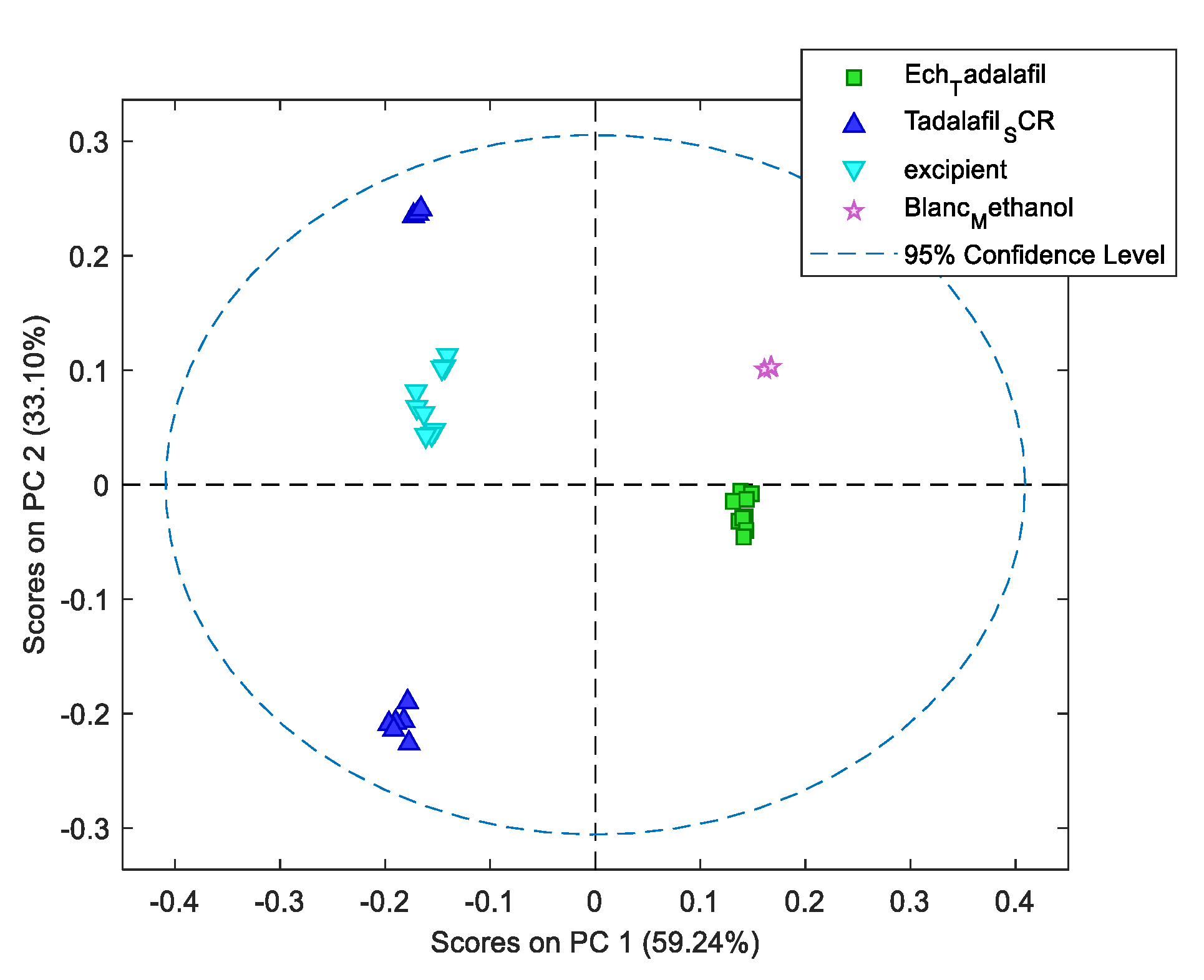
As can be seen in
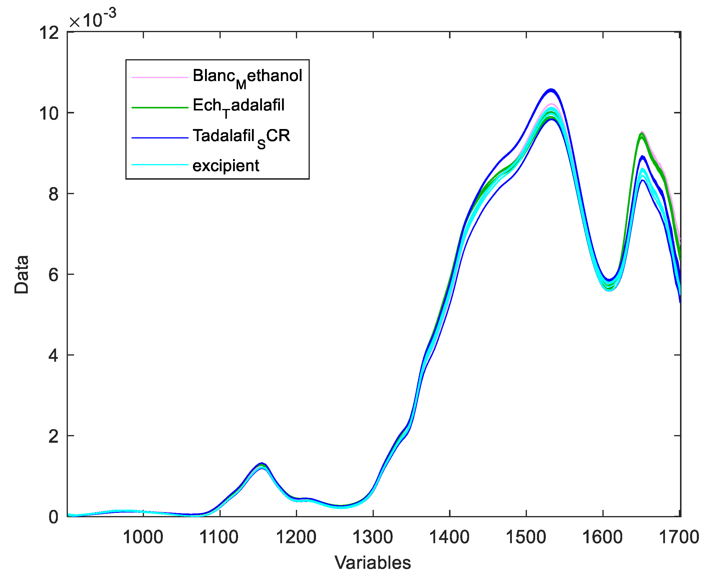
Figure 4, there is considerable variability between tadalafil tablet samples (green) and tadalafil standard samples (blue). What’s more, when the results are compared between the different samples, there is a significant difference in terms of spectral signature.
- 2
DD-SIMCA models
Due to the nature of NIR spectra (large, highly overlapping bands), it is recommended to use a qualitative model before the PLS regression model.
In this study, data-driven SIMCA (DD-SIMCA) was used to build qualitative identification models. DD-SIMCA is based on the construction of a principal component analysis (PCA) model of the target class, which in our case corresponds to the calibration spectra. In this way, the score distance (SD) and orthogonal distance (OD) can be calculated for each future spectrum, making it possible to determine, at a given confidence level, the acceptance zone for authentication of a specific brand. In our case, DD-SIMCA models were also used to distinguish X-1 Cialis from related (tadalafil-based) formulations but with different matrices.
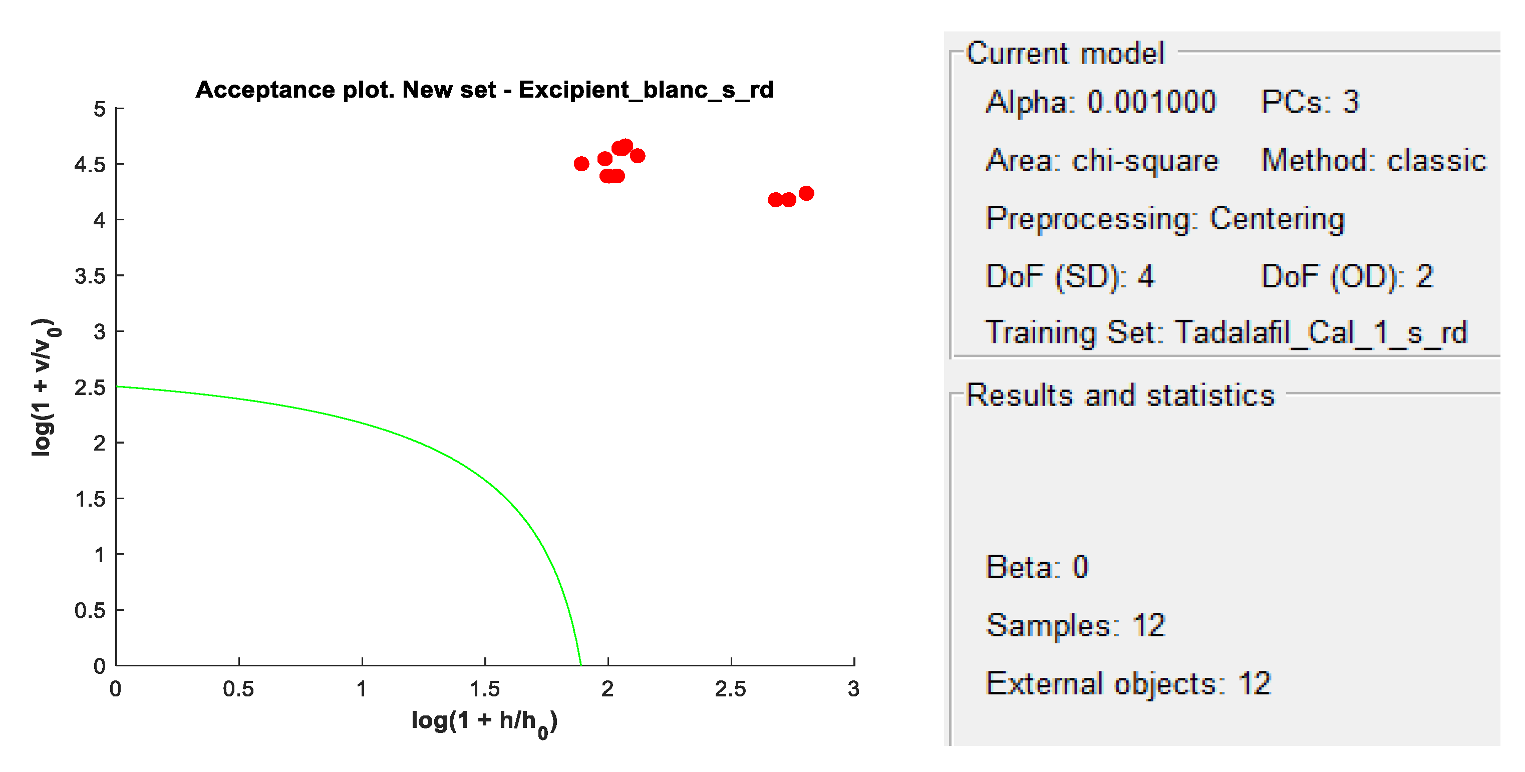
A placebo solution (excipient and blank) was also projected onto the DD-SIMCA model to ensure that X-1’s excipients did not interfere with the qualitative models.
Sensitivity was assessed using the new set (tadalafil validation set) on the DD-SIMCA models, using the following formula:
As a first validation criterion, the specificity of the method must be demonstrated. It is generally good practice to build a qualitative model before the quantitative one. This ensures that only spectra similar to those used for calibration are projected onto the regression model.
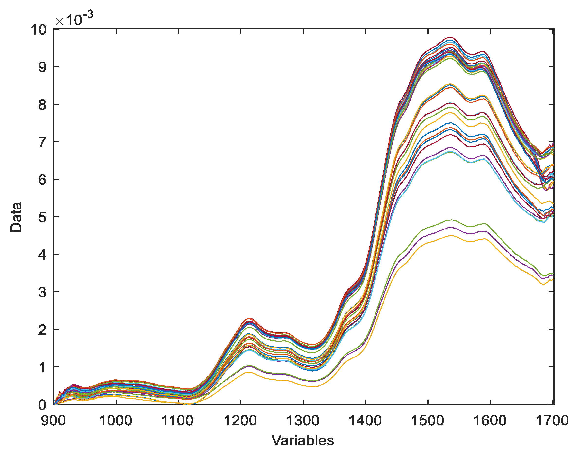
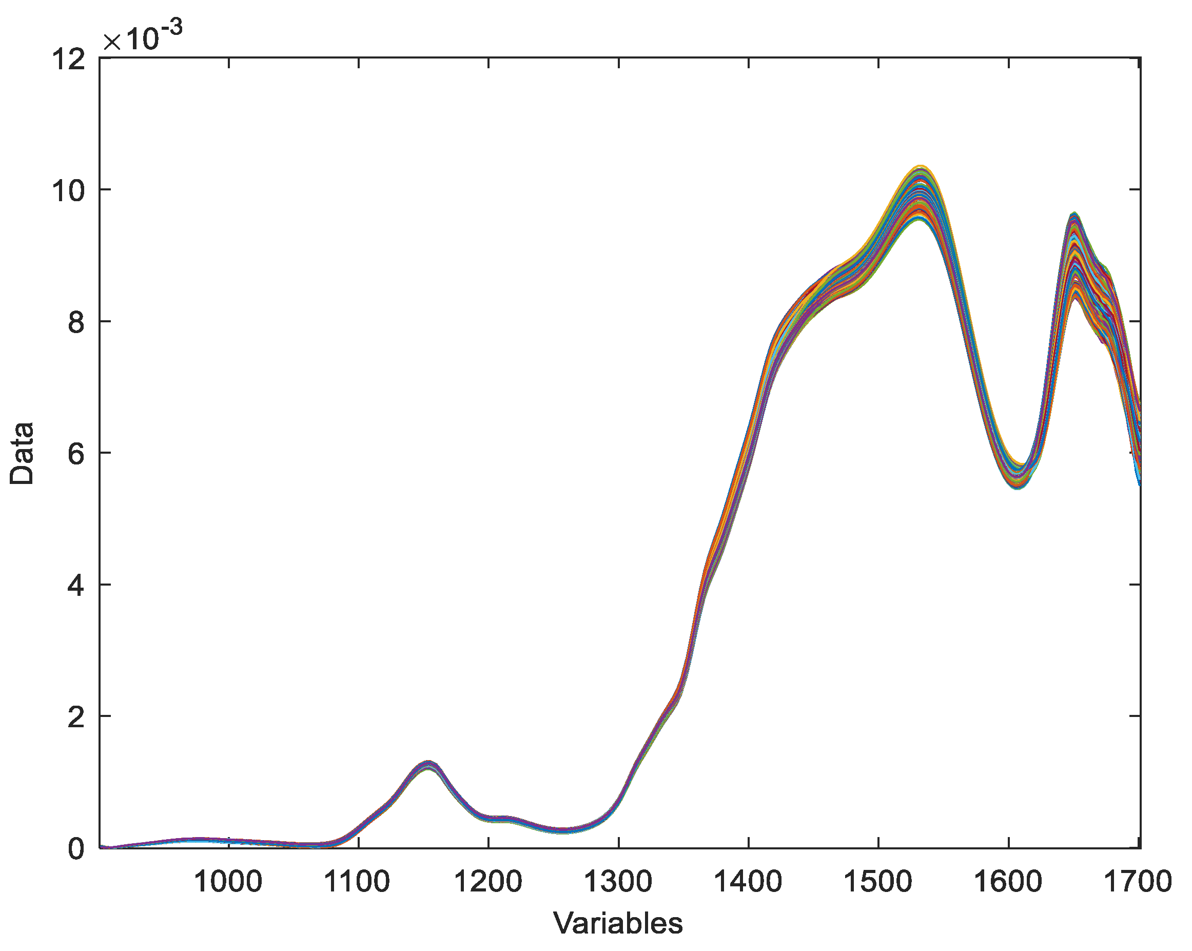
As can be seen, visual spectral correlation cannot be a reliable method of selectivity. Due to the very small differences between spectra, pre-processing methods using Savitzky-Golay derivatives improve spectral characteristics and facilitate discrimination of different APIs in SIMCA models. In addition, chemometric methods were used to help detect spectral dissimilarities between these samples. A single-class classification model was developed using the DD-SIMCA approach. The model parameters selected are listed in Table I, together with the associated sensitivity and specificity.
Table I.
Marketing Autorisation.
Table I.
Marketing Autorisation.
| Applicant |
Product name |
Manufacturer |
Origin country |
Authorization N° |
Registration N° |
Validity(yr) |
Peremption |
| KIM PHARMA |
X-1 20mg, capsule, bxe of 2. |
ETS KIM PHARMA |
DR.Congo |
MS.1253/10/05/DGM/0108/2016 |
May 2016 |
5 |
May 2021 |
| ELI LILLY NEDERLAND |
Cialis20mg |
Eli lilly Nederland |
Netherland |
EU/1/02/237/006 |
Nov 2012 |
10 |
Nov 2022 |
| |
Mon plaisir |
- |
- |
- |
- |
- |
- |
| |
Tadalanique |
- |
- |
- |
- |
- |
- |
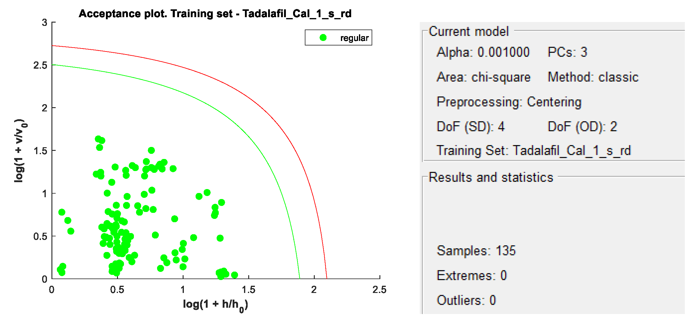
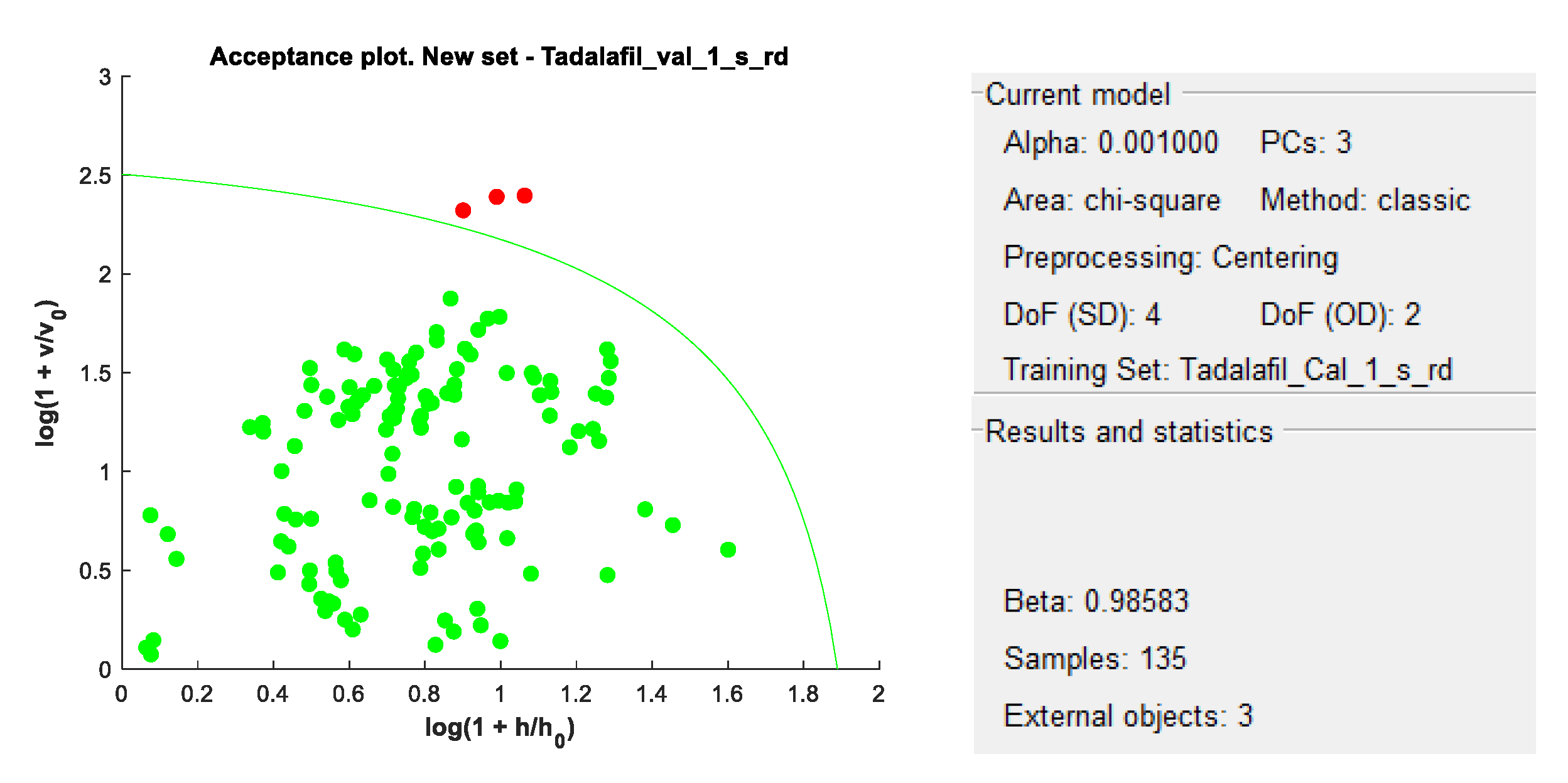
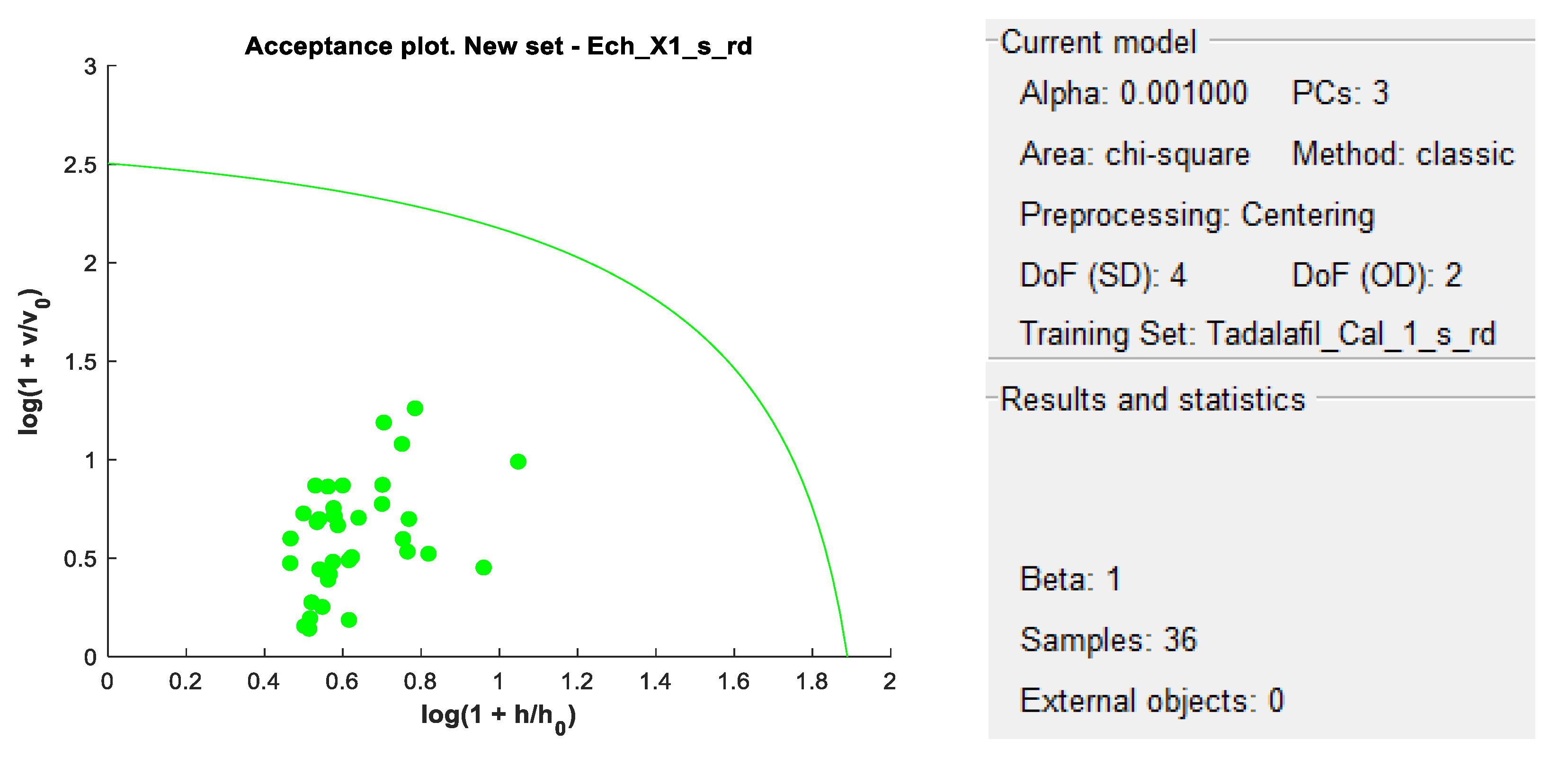
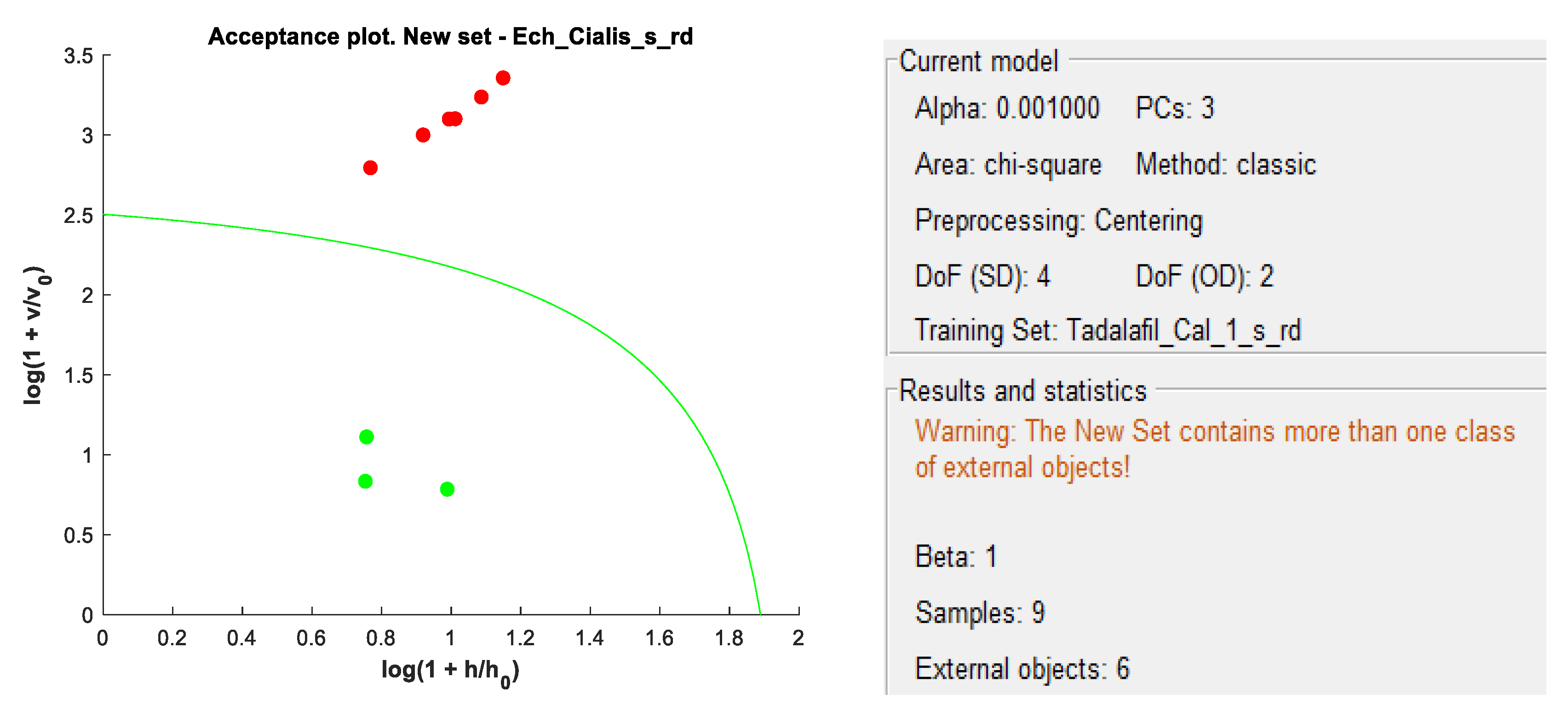
DD-SIMCA acceptance plots for calibration and validation data are shown in
Figure 5 and
Figure 6, while
Figure 7 and
Figure 8 show DD-SIMCA acceptance plots for X-1 and Cialis tablet data. The DD-SIMCA models applied to NIR data enabled perfect recognition of X-1 samples and perfect discrimination of placebo and, in part, Cialis samples. This confirms its applicability to systematically reject non-X-1 Tadalafil samples prior to quantitative analysis.
Nevertheless, performance showed a sensitivity of 97.7% for tadalafil validation samples; a specificity of 100% for matrix and a specificity of 33.3% for Cialis.
Table II.
Selected model parameters.
Table II.
Selected model parameters.
| Metric |
NIR-M-T1 |
| Spectral range |
1530-1642 nm |
| Preprocessing |
SG(1,2,15) + SNV + MC |
| # PC |
3 |
| A |
0.001 |
| Sn (VAL)% |
97.7 |
| Sp (Cialis)% |
33.3 |
| Sp (placebo)% |
100.0 |
SG: Savitzky-Golay (derivative, polynomial order, window size)
MC: Mean centering
SNV: Standard Normal Variable
Sn: Sensitivity
Sp: Specificity
PLS Analysis
Several PLS models have been built using different preprocessing methods, combinations of them and taking into account different numbers of latent variables.
Selecting an appropriate number of latent variables avoids under- or over-fitting the model.
A preselection of spectral ranges, preprocessing and number of latent variables was carried out with the PLS Toolbox model optimizer, using RMSEP as a quality criterion. The last few models selected were compared on the basis of accuracy profiles reflecting current use of the method.
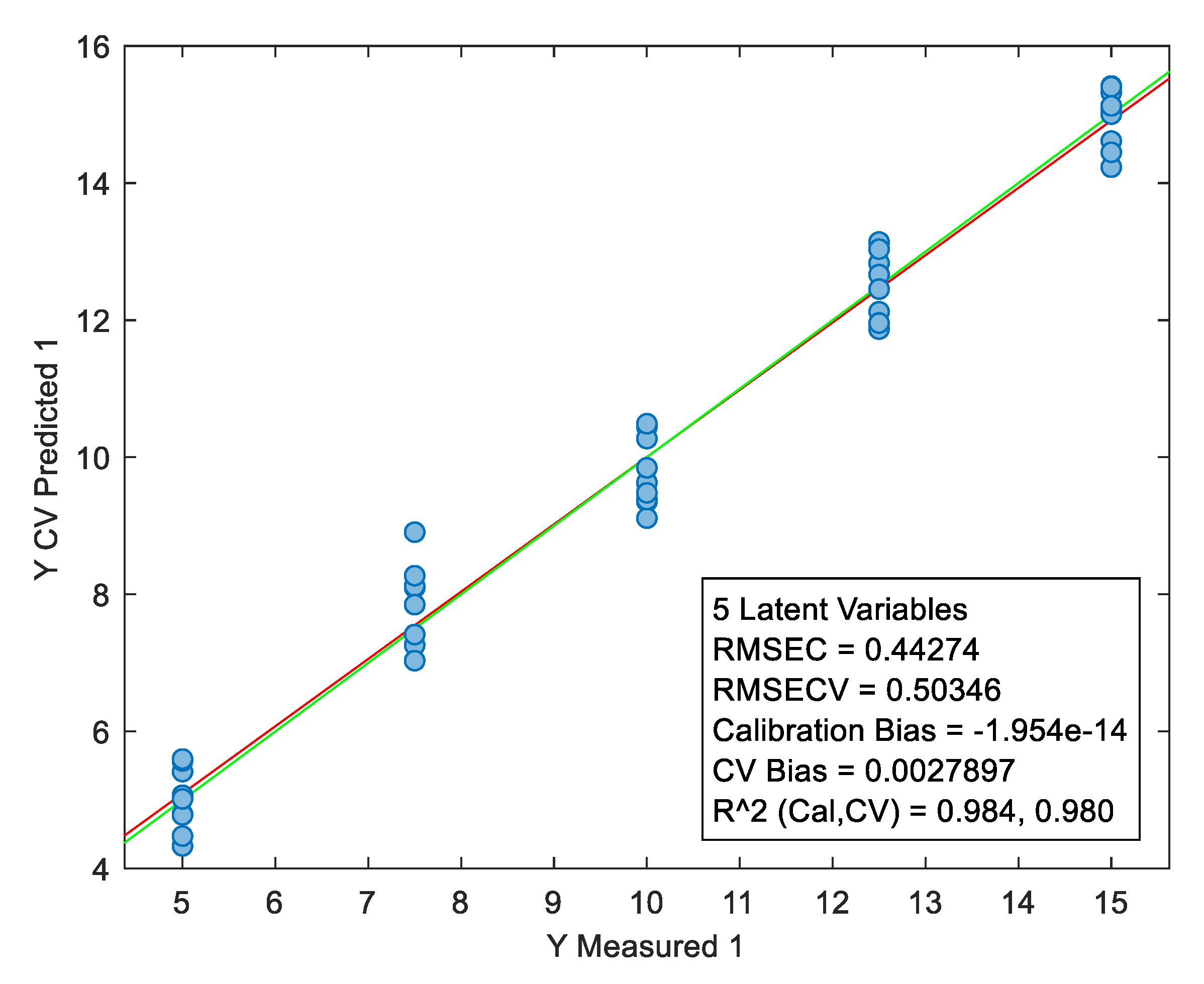
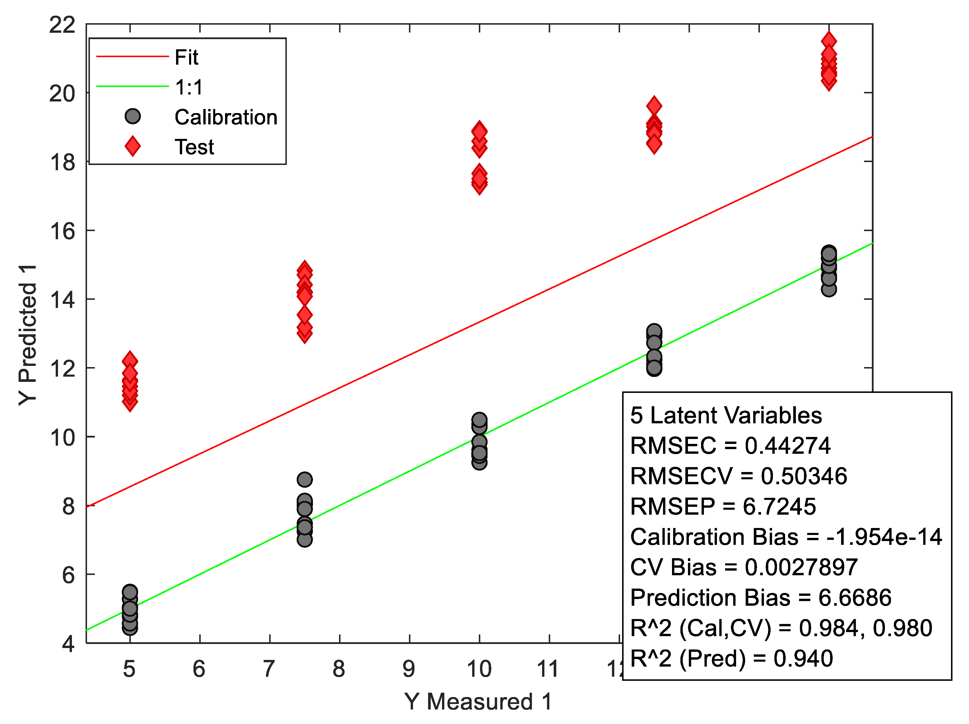
Figure 10.
Graph showing the characteristics of the PLS calibration model for NIR data.
Figure 10.
Graph showing the characteristics of the PLS calibration model for NIR data.
The wide dispersion of the relative error of different concentration levels can be explained by the fact that the matrix used contained excipients that could pass into the methanolic solution (due to the higher excipient/API ratio). This has a random impact on the amount of tadalafil present in the solution after the filtration step.After being developed, the PLS model was tested for its predictive ability on spectral data taken under multi-source environmental conditions (change in temperature and relative humidity). Unfortunately, a bias was observed when the developed model was used to predict validation samples measured under different conditions (see
Figure 6).
Table III.
Summary of spectral acquisition parameters.
Table III.
Summary of spectral acquisition parameters.
Figure 11.
Graph showing the characteristics of the PLS calibration model developed for the prediction of validation data.
Figure 11.
Graph showing the characteristics of the PLS calibration model developed for the prediction of validation data.
What’s more, when looking at the score graphs, the validation data are considered to be outliers in relation to the model, and unfortunately cannot be analyzed directly without correction.
The slope-bias correction SBC performed a linear-univariate model study between the predicted data and the standard data; then the linear model (taking into account the slope and y-intercept) was used to correct the predicted data using the following equation:
In some cases, this may be one of the alternative solutions for compensating for NIR spectral variations that may result from instrumental or environmental variability; for example, when samples and/or spectral measurements are significantly affected by changes in temperature, relative humidity or instrumental variability. What’s more, NIR-M-T1 portable instruments are still in the development phase, and do not have waterproof shells to protect the system from temperature and/or humidity variations. As a result, particular attention needs to be paid to their use in tropical zones, where there are strong seasonal variations in temperature and relative humidity.
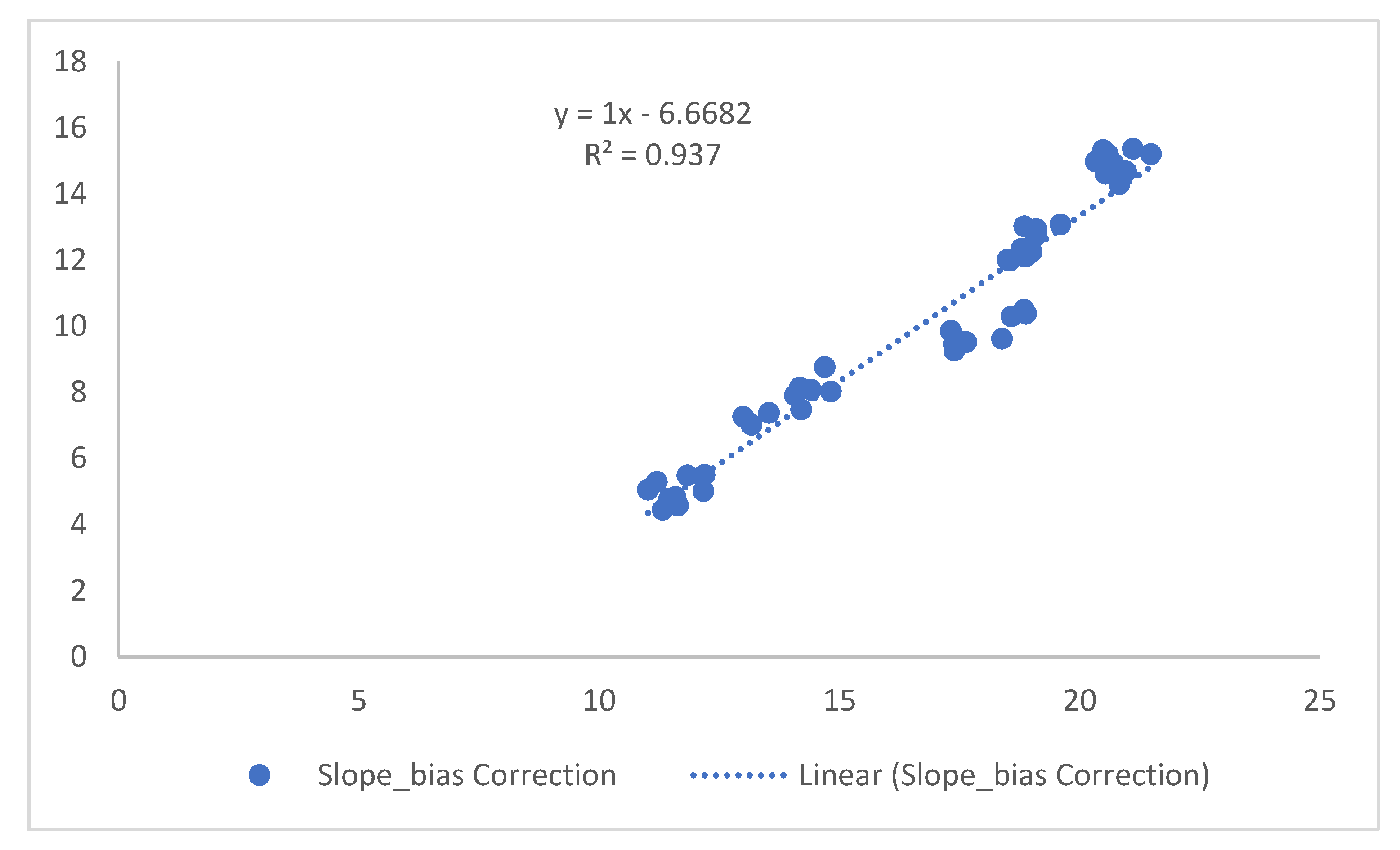
Figure 12.
Characteristics of the linear Y model.
Figure 12.
Characteristics of the linear Y model.
For SBC, the values of R
2 (coefficient of determination), (the slope of the linear fit) and y-intercept, using predicted versus calibration data, are presented in the linear equations in
Figure 8. The SBC corrected the bias observed when predicting standard tadalafil samples measured under different environmental conditions. The corrected predicted data enabled the model to be successfully validated in the tadalafil concentration range.
However, it would be interesting to test under different environmental conditions and check when a convergence is reached indicating the optimal condition to include in the overall modeling. Another approach could be the global modeling. This approach consists in adding the new variability resulting from the new data taken under different environmental conditions to the calibration set.
Validation
The NIR predictive model was validated using the total error approach with acceptance limits of ± 10% and a risk level of 5%.
All validation calculations were performed with E-noval 4.0b (PharmalexBelgium, Mont-saint-Guibert, Belgium).
Experiment plan
Validation standards are samples reconstituted in the matrix containing a known concentration and whose value is considered true by consensus.
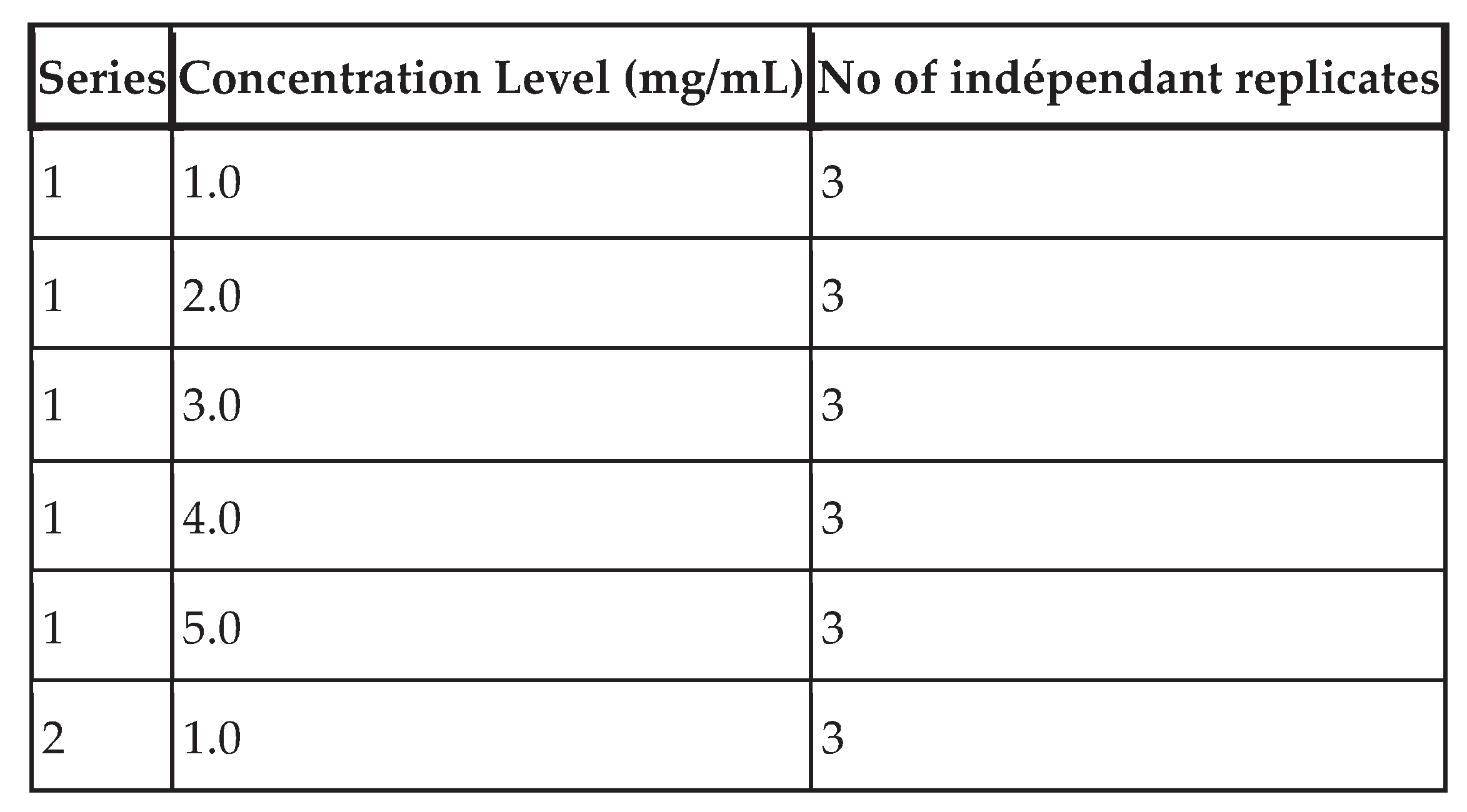
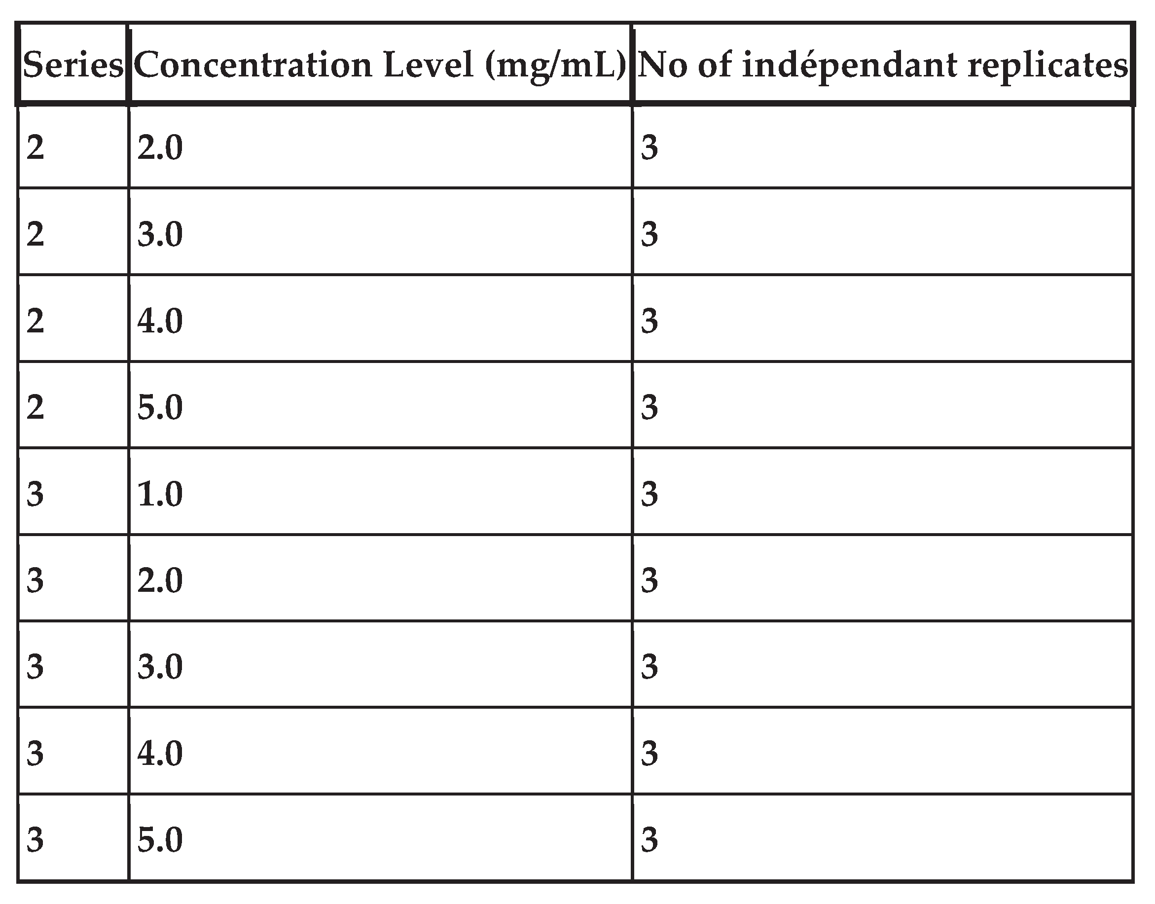
Table IV shows the number of validation standards per concentration level, the concentration levels considered and the different series performed.
Table IV.
Experiment plan.
Table IV.
Experiment plan.
Total number of observations: 45
Validation criteria study
Trueness
Trueness expresses the closeness of agreement between the mean value obtained from a large series of test results and an accepted reference value. Trueness gives an indication of systematic errors.
As shown in Table V, trueness is expressed in terms of absolute bias (mg/mL), relative bias (%) or recovery rate (%) for each concentration level of the validation standards.
Precision
Precision expresses the closeness of agreement between a series of measurements taken from multiple replicates of the same homogeneous sample under prescribed conditions. It provides information on random error and is assessed at two levels: repeatability and intermediate precision.
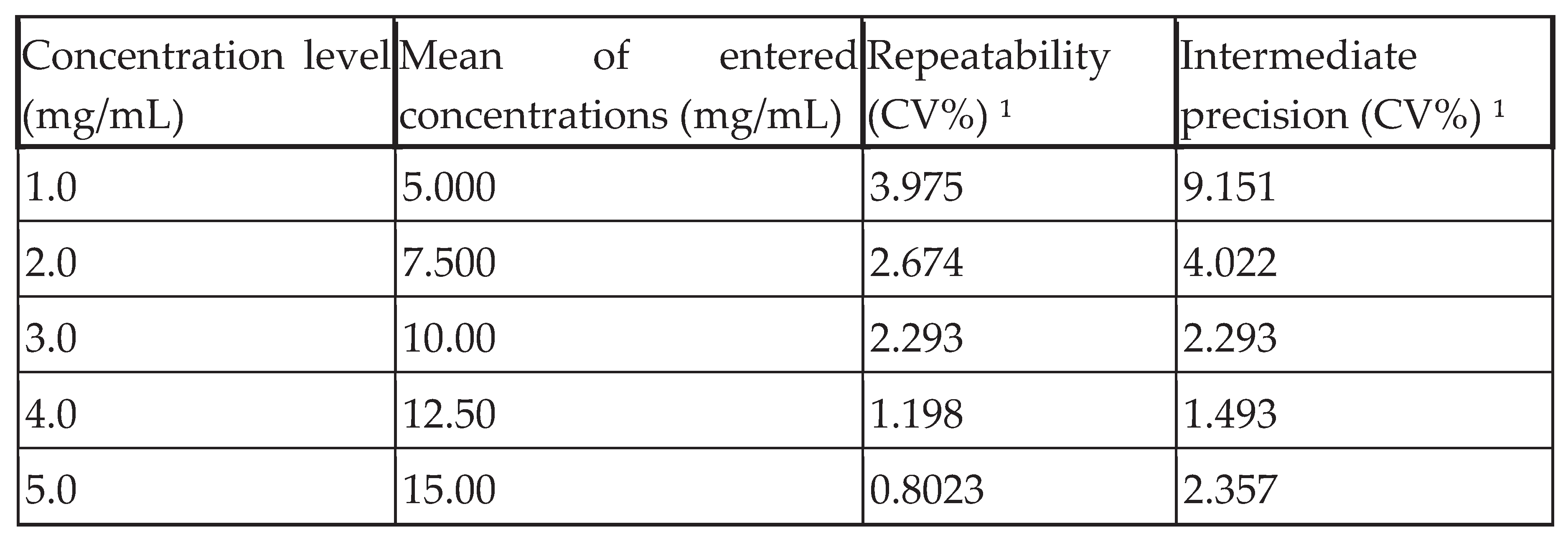
As shown in Table VI, precision (repeatability and intermediate precision) can be expressed in terms of standard deviation (SD) and coefficient of variation (CV).
Table VI.
Repeatability and relative intermediate precision.
Table VI.
Repeatability and relative intermediate precision.
CVs in % of Repeatability and Intermediate precision were obtained by dividing the standard deviation (SD) obtained by the corresponding mean of the introduced concentrations.
The precision of this method was assessed at two levels: repeatability and intermediate precision. The coefficient of variation (CV) was used as an expression of this precision.
For good method fidelity, the percentage CV must not exceed 2.000 at all concentration levels studied. This explains the good precision only at levels 4.0 and 5.0; repeatability and intra-day intermediate precision are very good considering only these two levels.
Accuracy
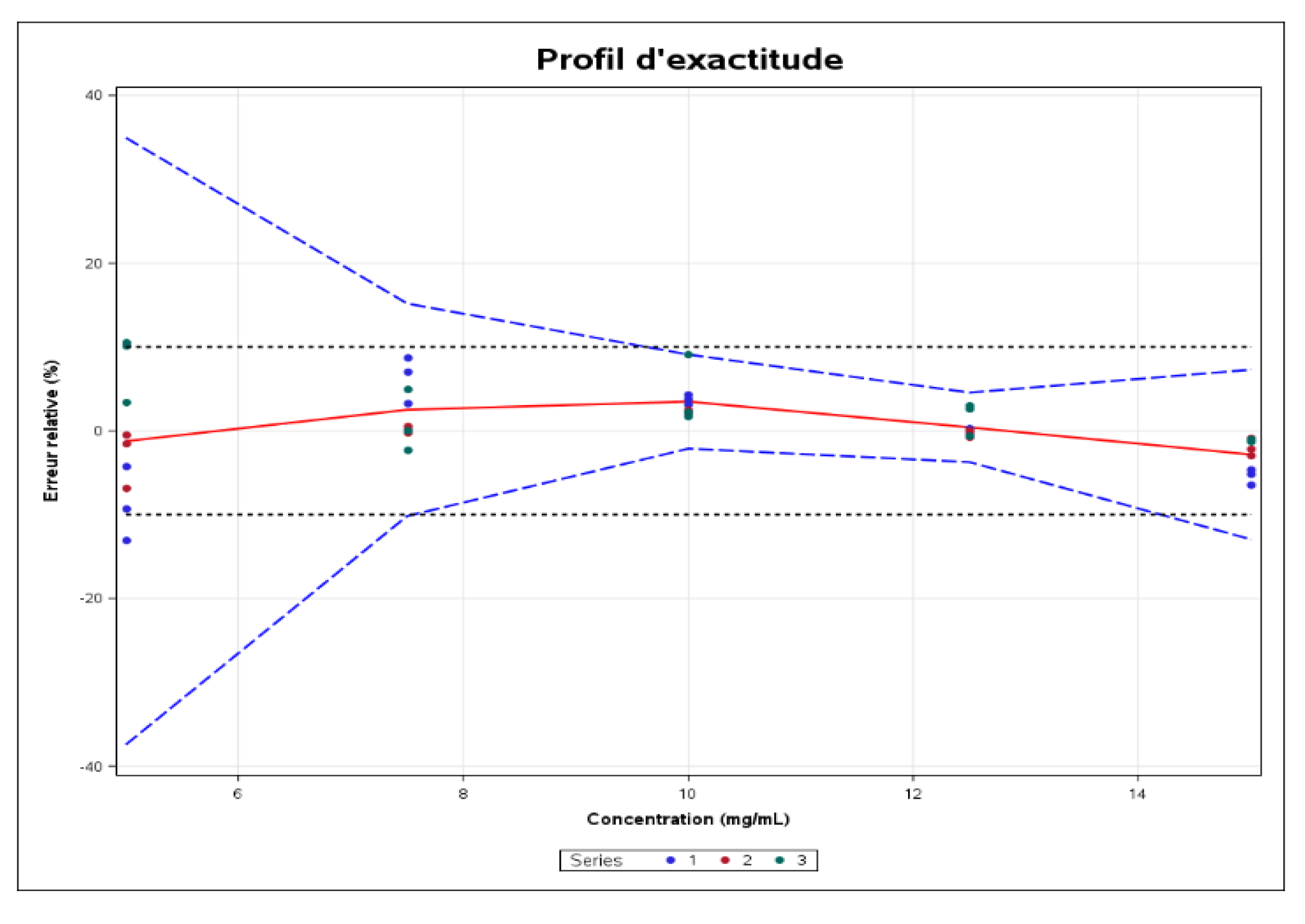
Accuracy expresses the closeness of agreement between the test result and the reference value accepted as such, also known as the “conventionally true value”. Accuracy takes into account the total error, i.e., the systematic error and the random error associated with the result. Consequently, accuracy is the sum of trueness and precision. It is estimated from the accuracy profile shown in
Figure 13.
Acceptance limits have been set at ± 10%, in line with the objective of the analytical procedure (USP).
Figure 13.
Accuracy profile.
Figure 13.
Accuracy profile.
The solid red line represents the relative bias, the dashed blue lines define the limits of the tolerance interval expected at beta level, and the dashed black lines are the acceptance limits. The dots represent the relative error of the results and are plotted against their target concentrations.
Linearity
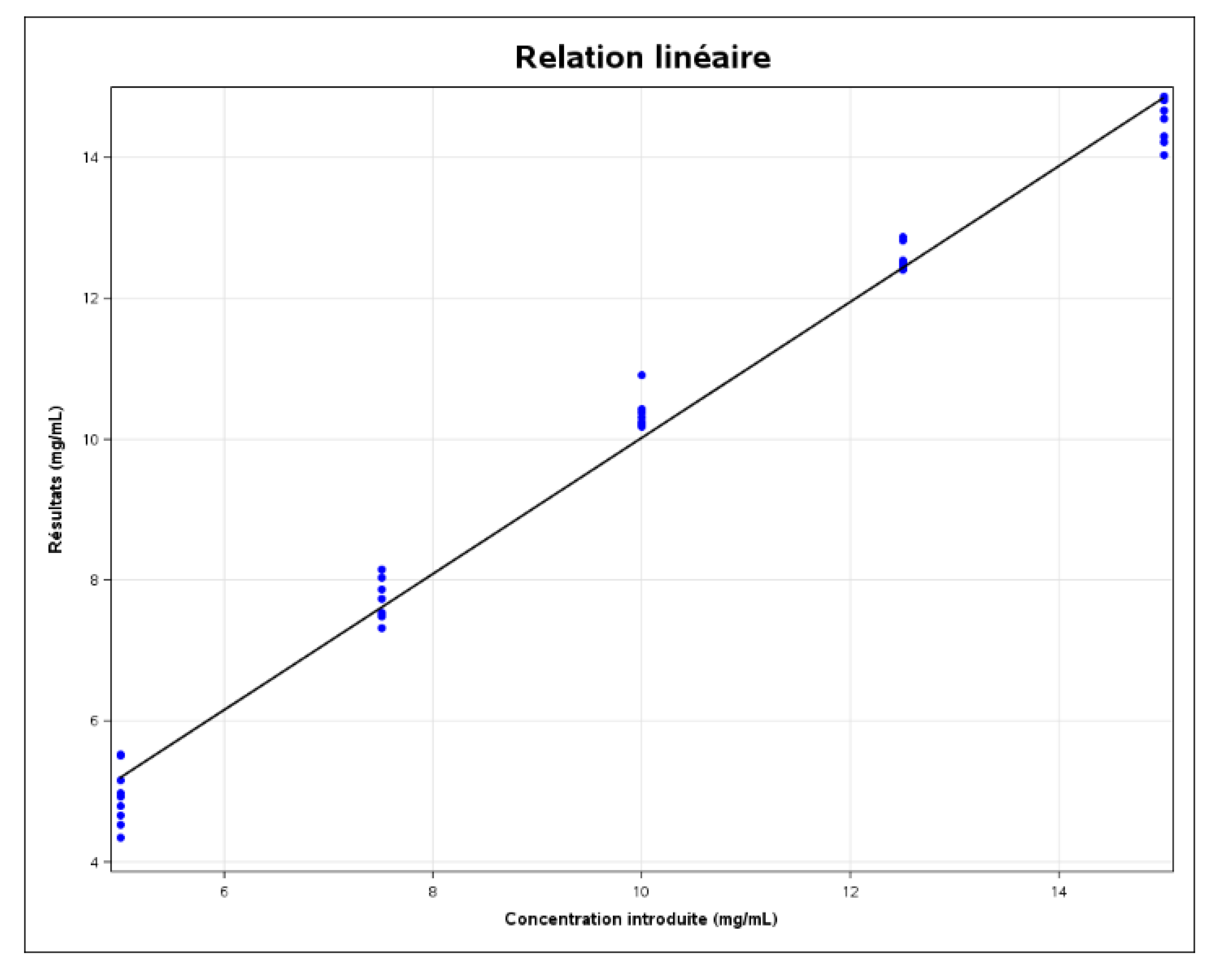
The linearity of an analytical method is its ability, within a certain assay interval, to obtain results directly proportional to the analyte concentration in the sample. A linear regression model (see
Figure 7:1) was fitted to the results calculated as a function of the concentrations introduced, in order to obtain the following equation:
Where Y = results (mg/mL)
And X = concentrations introduced (mg/mL)
The coefficient of determination (r2) is 0.9890.
The correlation coefficient (r) is 0.9945.
Figure 14.
Relationship between introduced concentrations and results.
Figure 14.
Relationship between introduced concentrations and results.
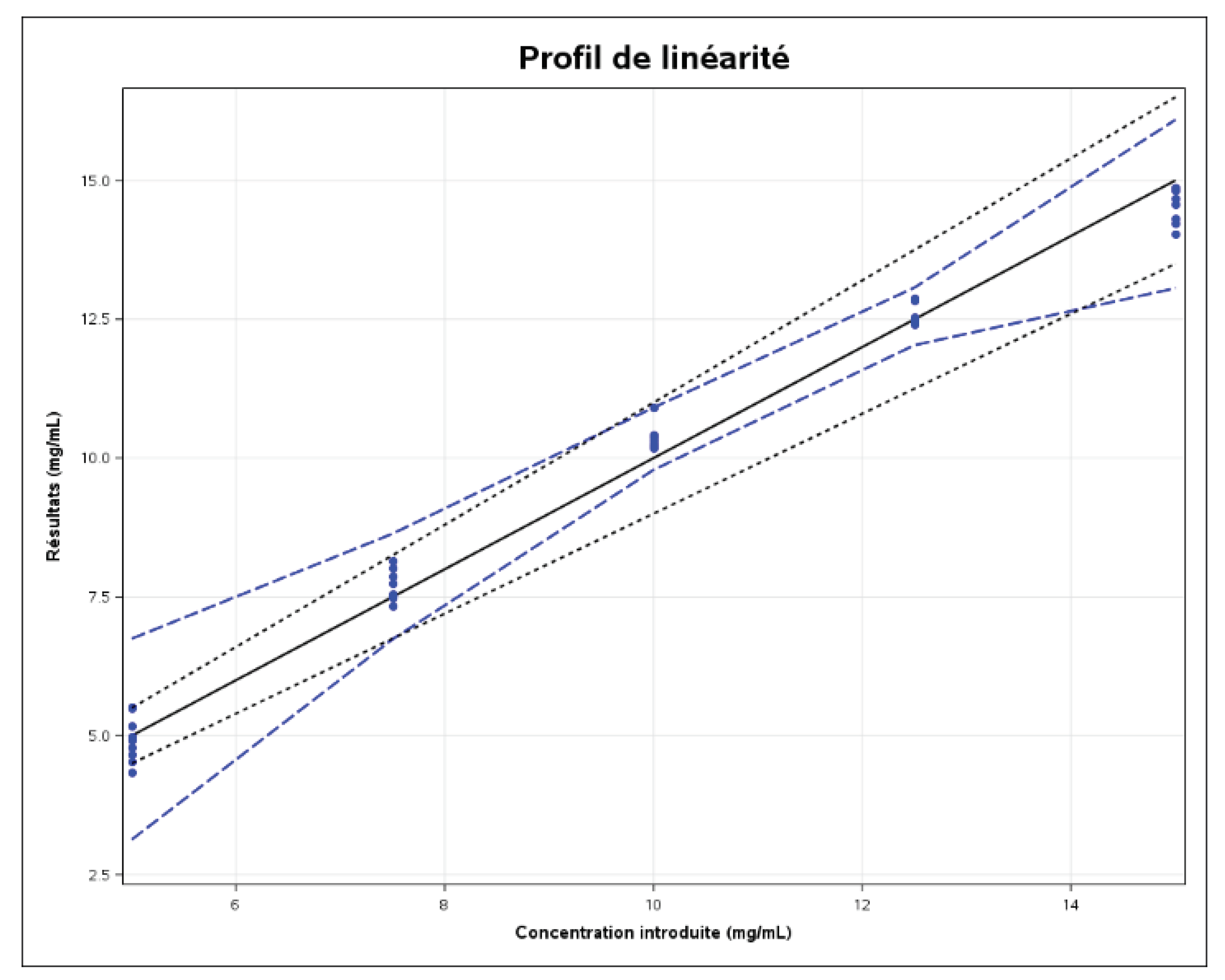
Figure 15.
linearity graph.
Figure 15.
linearity graph.
The solid black line is the identity line (Y=X). The limits represented by the dashed blue lines on the graph correspond to the accuracy profile, i.e., the “beta-expectation” tolerance limits expressed in absolute values.
In order to demonstrate the linearity of the method, the approach based on the expected tolerance interval at beta level, expressed as an absolute value, can be used and is illustrated in the previous figure. As the figure shows, the linearity of the method is not exactly valid. This is due to the fact that R2 (0.989) is not close to 1. In this case, we say that there is no good agreement between the concentrations introduced and the concentrations calculated for certain levels.
