You are currently viewing a beta version of our website. If you spot anything unusual, kindly let us know.

Preprint

Article

Modeling Pandemic Vaccine with Saturated Incidence Rate Based on Disease Induced Death

Altmetrics

Downloads

Views

Comments

Odriozola Vazquez^*

This version is not peer-reviewed

Abstract

This paper presents a comprehensive analysis of the SEIRS COVID-19 pandemic model with saturated incidence rate. By modifying the existing model and proposing a new simplified version, we investigate the dynamics of disease transmission, including the impact of saturation terms on disease spread. Through stability analysis at disease-free and endemic equilibria, we aim to enhance understanding of the spread of COVID-19 and inform effective control strategies. Drawing on mathematical models and epidemiological insights, this study contributes to the ongoing efforts to combat the global pandemic.

Keywords:

Subject: Computer Science and Mathematics - Applied Mathematics

Introduction

Coronavirus Disease (COVID-19) is an infectious disease caused by a newly discovered coronavirus. Most people infected with the (COVID-19) virus will experience mild to moderate respiratory illness and recover without requiring special treatment. Older people and those with underlying medical problems like cardiovascular disease, diabetes, chronic respiratory disease and cancer are more likely to develop serious illness. The best way to prevent and slow down transmission is to be well informed about (COVID-19) virus; the disease is causes and how it spreads.

At this time, there are no specific vaccines or treatments for (COVID-19). However, there are many ongoing clinical trials evaluating potential treatments. WHO (World Health Organization) will continue to provide updated information as soon as clinical findings become available (WHO).

[1,2] studied mathematical model for malaria transmission dynamics on human and mosquito population with non-linear forces of infectious disease and Malaria model with stage-structured mosquitoes. Dynamics of multiple species and strains of malaria together with on the numerical simulation of the effect of saturation terms on the SEIRS epidemic model was analyzed in [3,4]. [5,6,7] considered the dynamical behavior of epidemiological models with non linear incidence rate and Reproduction numbers and Sub-threshold endemic equilibria for compartmental models of disease transmission with Permanence and Extinction for a non-autonomous SEIRS epidemic model. [8] Studied the Lyapunov functions and global properties for SEIR and SEIS epidemic models. Likewise, in [9] the Stability analysis of an HIV/AIDS epidemic model with treatment was identified.

In this paper, the work of Kolawole M.K. [10] was extended to incorporate vaccine (treatment rate). We present our results in the form of Basic Reproduction Number

R_{0}

using Next Generation Matrix Method and data security [13,14,15,16,17]. Theorems are used to prove the Local and Global Stabilities of disease free and endemic equilibria. With the numerical simulations, the results showed the effect of Vaccine (treatment rate), transmission rate and disease induced death rate in the model.

2. The Basic Mathematical Model

In this paper, model of Kolawole M.K. (2016) was modified

The Existing model of KOLAWOLE (2016)

\begin{array}{l} \frac{d S}{d t} = \land - \frac{β S I}{1 + m_{1} S + m_{2} I} - μ S + δ R \\ \frac{d E}{d t} = \frac{β S I}{1 + m_{1} S + m_{2} I} - (μ + ε) E \\ \frac{d I}{d t} = ε E - (μ + γ + d) I \\ \frac{d R}{d t} = γ I - (μ + δ) R \end{array}

(1)

Proposed model

\begin{array}{l} \frac{d S}{d t} = \land - \frac{β S I}{1 + m_{1} S + m_{2} I} - μ S + δ R \\ \frac{d E}{d t} = \frac{β S I}{1 + m_{1} S + m_{2} I} - (μ + ε) E \\ \frac{d I}{d t} = ε E - (μ + γ + d + v) I \\ \frac{d R}{d t} = γ I - (μ + δ) R \end{array}

(2)

For the purpose of simplicity, the new Proposed model becomes;

\begin{array}{l} \frac{d S}{d t} = \land - \frac{β S I}{1 + a S + b I} - μ S + δ R \\ \frac{d E}{d t} = \frac{β S I}{1 + a S + b I} - (μ + ε) E \\ \frac{d I}{d t} = ε E - (μ + γ + d + v) I \\ \frac{d R}{d t} = γ I - (μ + δ) R \end{array}

(3)

3. Disease Free Equilibrium (DFE)

At disease free equilibrium

Ι = 0, E = 0, R = 0

\begin{array}{l} \land - \frac{β S I}{1 + a S + b I} - μ S + δ R = 0 \\ \land - μ S = 0 \\ S = \frac{\land}{μ} \\ (S, E, I, R) = (\frac{\land}{μ}, 0, 0, 0) \end{array}

4. Endemic Equilibrium

At Endemic Equilibrium,

I \neq 0,

To get

R^{*}

\begin{array}{l} γ I^{*} - (μ + δ) R^{*} = 0 \\ γ I^{*} = (μ + d) R^{*} \\ R^{*} = \frac{γ I^{*}}{μ + δ} \end{array}

(4)

Then

S^{*}

gives,

\begin{array}{l} \frac{β S^{*} I^{*}}{1 + a S^{*} + b I^{*}} - (μ + ε) E^{*} = 0 \\ \frac{β S^{*} I^{*}}{1 + a S^{*} + b I^{*}} = (μ + ε) E^{*} \\ β S^{*} I^{*} = (1 + a S^{*} + b I^{*}) (μ + ε) E^{*} \\ β S^{*} I^{*} = a S^{*} (μ + ε) E^{*} + (1 + b I^{*}) (μ + ε) E^{*} \\ β S^{*} I^{*} - a S^{*} (μ + ε) E^{*} = (1 + b I^{*}) (μ + ε) E^{*} \\ S^{*} = \frac{(1 + b I^{*}) (μ + ε) E^{*}}{β I^{*} - a (μ + ε) E^{*}} \end{array}

(5)

Then compartment

I^{*}

becomes,

\begin{array}{l} \land - \frac{β S^{*} I^{*}}{1 + a S^{*} + b I^{*}} - μ S^{*} + δ R^{*} = 0 \\ \land - μ S^{*} + δ R^{*} = \frac{β S^{*} I^{*}}{1 + a S^{*} + b I^{*}} \\ (\land - μ S^{*} + δ R^{*}) (1 + a S^{*} + b I^{*}) = β S^{*} I^{*} \\ (\land - μ S^{*} + δ R^{*}) (1 + a S^{*}) + (\land - μ S^{*} + δ R) b I^{*} = β S^{*} I^{*} \\ (\land - μ S^{*} + δ R^{*}) (1 + a S^{*}) = β S^{*} I^{*} - (\land - μ S^{*} + δ R) b I^{*} \\ I^{*} = \frac{(\land - μ S^{*} + δ R^{*}) (1 + a S^{*})}{β S^{*} - b (\land - μ S^{*} + δ R^{*})} \end{array}

(6)

Then

E^{*}

becomes,

\begin{array}{l} \begin{array}{l} ε E^{*} - (μ + γ + d + v) I^{*} = 0 \\ ε E^{*} = (μ + γ + d + v) I^{*} \end{array} \\ E^{*} = \frac{(d + α + m) I^{*}}{ε} \end{array}

(7)

5. Basic Reproduction Number $R_{0}$

Using next generation matrix,

R_{0} = F \times V^{- 1}

F = [\begin{matrix} \frac{β \land}{μ + a \land} & 0 \\ 0 & 0 \end{matrix}] and V = [\begin{matrix} 0 & (μ + ε) \\ (μ + γ + d + v) & - ε \end{matrix}]

The inverse of

V

is obtained as

V^{- 1} = \frac{- 1}{(μ + ε) (μ + γ + d + v)} [\begin{matrix} - ε & (μ + ε) \\ (μ + γ + d + v) & 0 \end{matrix}]

Hence,

\begin{array}{l} R_{0} = F . V^{- 1} = [\begin{matrix} \frac{β \land}{μ + a \land} & 0 \\ 0 & 0 \end{matrix}] [\begin{matrix} \frac{ε}{(μ + ε) (μ + γ + d + v)} & \frac{- 1}{(μ + γ + d + v)} \\ \frac{- 1}{(μ + ε)} & 0 \end{matrix}] \\ R_{0} = [\begin{matrix} \frac{β \land ε}{(μ + a \land) (μ + ε) (μ + γ + d + v)} & 0 \\ 0 & 0 \end{matrix}] \end{array}

The equation with the dominant Eigen value becomes,

R_{0} = \frac{β \land ε}{(μ + a \land) (μ + ε) (μ + γ + d + v)}

(8)

6. Local Stability of Disease Free Equilibrium

We Linearize the system of equation in (3) by setting

\begin{array}{l} S - S_{1} = x, E = E, I = I, R = R \\ S = x + S_{1} \end{array}

Where

S_{1} = \frac{\land}{μ}

Therefore,

\begin{array}{l} \frac{d S}{d t} = \land - \frac{β S I}{1 + a S + b I} - μ S + δ R \\ \frac{d E}{d t} = \frac{β S I}{1 + a S + b I} - (μ + ε) E \\ \frac{d I}{d t} = ε E - (μ + γ + d + v) I \\ \frac{d R}{d t} = γ I - (μ + δ) R \end{array}

(9)

The Linearized system gives,

\begin{array}{l} \frac{d x}{d t} = - μ x + \frac{β \land}{μ} (\frac{a \land}{μ} - 1) I + Non linear terms \\ \frac{d E}{d t} = \frac{β \land}{μ} (1 - \frac{a \land}{μ}) I - (μ + ε) E + Non linear terms \\ \frac{d I}{d t} = ε E - (μ + γ + d + v) I + Non linear terms \\ \frac{d R}{d t} = γ I - (μ + δ) R + Non linear terms \end{array}

(10)

The Jacobian matrix of equation (10) becomes,

J (E_{0}) = [\begin{matrix} - μ & 0 & \frac{β \land}{μ} (\frac{a \land}{μ} - 1) & δ \\ 0 & - (μ + ε) & \frac{β \land}{μ} (1 - \frac{a \land}{μ}) & 0 \\ 0 & ε & - (μ + γ + d + v) & 0 \\ 0 & 0 & γ & - (μ + δ) \end{matrix}]

Then the determinant

|A - I λ| = 0

becomes,

J (E_{0}) = |\begin{matrix} - μ & 0 & \frac{β \land}{μ} (\frac{a \land}{μ} - 1) & δ \\ 0 & - (μ + ε) & \frac{β \land}{μ} (1 - \frac{a \land}{μ}) & 0 \\ 0 & ε & - (μ + γ + d + v) & 0 \\ 0 & 0 & γ & - (μ + δ) \end{matrix}| = 0

(11)

The solutions give,

λ_{1} = - μ λ_{2} = - (μ + δ)

λ_{3} = \frac{1}{μ} (- \frac{1}{2} μ d - \frac{1}{2} μ ε - \frac{1}{2} μ γ - μ^{2} - \frac{1}{2} μ v + \frac{1}{2} \sqrt{D})

λ_{3} = \frac{1}{μ} (- \frac{1}{2} μ d - \frac{1}{2} μ ε - \frac{1}{2} μ γ - μ^{2} - \frac{1}{2} μ v + \frac{1}{2} \sqrt{D})

Where

D = \sqrt{- 4 \land^{2} a β ε + 4 \land β ε μ + d^{2} μ^{2} - 2 d ε μ^{2} + 2 d γ μ^{2} + 2 d μ^{2} v + ε^{2} μ^{2} - 2 ε γ μ^{2} - 2 ε μ^{2} v + γ^{2} μ^{2} + 2 γ μ^{2} v + μ^{2} v^{2}}

Theorem:

R_{0} < \frac{μ^{2}}{μ^{2} - \land^{2} a^{2}} < 1,

therefore, the disease free equilibrium is Locally asymptotically Stable and if

R_{0} > \frac{μ^{2}}{μ^{2} - \land^{2} a^{2}} > 1,

therefore the disease equilibrium is unstable.

Proof:

The characteristic equation from equation (11) gives

λ_{1} = - μ λ_{2} = - (μ + δ)

λ_{1} = - μ λ^{2} + (2 μ + ε + γ + d + v) λ + (μ + ε) (μ + γ + d + v) (1 - (\frac{μ^{2} - \land^{2} a^{2}}{μ^{2}}) R_{0}) = 0

(12)

By Descartes rule of signs, it shows that there are no signs changes in equation (12), If

R_{0} < \frac{μ^{2}}{μ^{2} - \land^{2} a^{2}} < 1,

Implies that there are no positive root in equation (12). Now, if

λ

is replaced with

- λ

in equation (12), we have

λ^{2} - (2 μ + ε + γ + d + v) λ + (μ + ε) (μ + γ + d + v) (1 - (\frac{μ^{2} - \land^{2} a^{2}}{μ^{2}}) R_{0}) = 0

(13)

There are two sign changes in the above equilibrium; hence it has two exact negative roots of

R_{0} < \frac{μ^{2}}{μ^{2} - \land^{2} a^{2}} < 1,

Hence, the Eigen values of equation (13) are all negative i.e.

λ_{3} = \frac{1}{μ} (- \frac{1}{2} μ d - \frac{1}{2} μ ε - \frac{1}{2} μ γ - μ^{2} - \frac{1}{2} μ v + \frac{1}{2} \sqrt{D})

λ_{4} = \frac{1}{μ} (- \frac{1}{2} μ d - \frac{1}{2} μ ε - \frac{1}{2} μ γ - μ^{2} - \frac{1}{2} μ v - \frac{1}{2} \sqrt{D})

Since

λ_{1}, λ_{2}, λ_{3} a n d λ_{4}

are all negative, it follows that the disease free equilibrium is Locally Asymptotically stable.

Now, if

R_{0} > \frac{μ^{2}}{μ^{2} - \land^{2} a^{2}} > 1,

in equation (12) then,

It shows that only one sign will be positive then the other part will be negative.

Now, if

λ

is replaced with

- λ

in equation (13), we say

λ^{2} + (2 μ + ε + γ + d + v) λ - (μ + ε) (μ + γ + d + v) (1 - (\frac{μ^{2} - \land^{2} a^{2}}{μ^{2}}) R_{0}) = 0

(14)

There are one sign changes in the above equilibrium; hence it has one exact negative root. Also, we replace

λ

w i t h ​ - λ w e h a v e

λ^{2} - (2 μ + ε + γ + d + v) λ + (μ + ε) (μ + γ + d + v) (1 - (\frac{μ^{2} - \land^{2} a^{2}}{μ^{2}}) R_{0}) = 0

(15)

There is just a sign change, which shows that there is one negative root. That is, not all Eigen Values are negative, hence the disease free equilibrium point

(S, E, I, R) = (\frac{\land}{μ}, 0, 0, 0)

is unstable If

R_{0} > \frac{μ^{2}}{μ^{2} - \land^{2} a^{2}} > 1.

7. Global Stability of Disease Free Equilibrium

We consider the Lyapunov function,

\begin{array}{l} V = ε E^{'} + (μ + ε) I^{'} (16) \\ \frac{d V}{d t} = ε \frac{d E}{d t} + (μ + ε) \frac{d I}{d t} \end{array}

(16)

At disease free equilibrium, we have

(S, E, I, R) = (\frac{\land}{μ}, 0, 0, 0)

Then we have,

\begin{array}{l} \frac{d V}{d t} = μ [\frac{β S I}{1 + a S + b I} - (μ + ε) E] + (d + μ) [ε E - (μ + γ + d + v) I] \\ \frac{d v}{d t} = (μ + ε) (μ + γ + d + v) [\frac{β \land ε}{(μ + a \land) (μ + ε) (μ + γ + d + v)} - 1] I \end{array}

\begin{array}{l} \frac{d V}{d t} = μ [\frac{β S I}{1 + a S + b I} - (μ + ε) E] + (d + μ) [ε E - (μ + γ + d + v) I] \\ \frac{d v}{d t} = (μ + ε) (μ + γ + d + v) [\frac{β \land ε}{(μ + a \land) (μ + ε) (μ + γ + d + v)} - 1] I \\ L^{1} = (μ + ε) (μ + γ + d + v) [R_{0} - 1] \leq 0 \\ I f R_{0} \leq 1 \\ L^{1} \leq 0 \end{array}

(17)

Hence, the Disease Free Equilibrium is Globally Asymptotically Stable.

8. Local Stability of Endemic Equilibrium

Let

\begin{array}{l} S - S^{*} = w, E - E^{*} = x, I - I^{*} = y, R - R^{*} = z \\ \frac{d s}{d t} = \frac{d w}{d t}, \frac{d E}{d t} = \frac{d x}{d t}, \frac{d I}{d t} = \frac{d y}{d t}, \frac{d R}{d t} = \frac{d z}{d t} \end{array}

Then, we have

\begin{array}{l} \frac{d w}{d t} = (- β I^{*} + 2 β I^{*} a S^{*} + β I^{*^{2}} b - μ) w + (- β S^{*} + β S^{*} a + 2 β S^{*} b I^{*}) y + δ z + non linear terms \\ \frac{d x}{d t} = (β I^{*} - 2 β I^{*} a S^{*} - {β I^{*}}^{2} b) w + (β S^{*} - β S^{*} a - 2 β S^{*} b I^{*}) y - (μ + ε) x + non linear terms \\ \frac{dy}{dt} = ε x - (μ + γ + d + v) y + non linear terms \\ \frac{dz}{dt} = γ y - (μ + δ) z + non linear terms \end{array}

(18)

The Jacobian Matrix in (18) becomes,

(\dot{\begin{array}{l} w \\ \dot{\begin{array}{l} x \\ \dot{\begin{array}{l} y \\ \dot{z} \end{array}} \end{array}} \end{array}}) = (\begin{matrix} (- β I^{*} + 2 β I^{*} a S^{*} + β I^{*^{2}} b - μ) & 0 & (- β S^{*} + β S^{*} a + 2 β S^{*} b I^{*}) & δ \\ (β I^{*} - 2 β I^{*} a S^{*} - {β I^{*}}^{2} b) & - (μ + ε) & (β S^{*} - β S^{*} a - 2 β S^{*} b I^{*}) & 0 \\ 0 & ε & - (μ + γ + d + v) & 0 \\ 0 & 0 & γ & - (μ + δ) \end{matrix}) (\begin{array}{l} w \\ x \\ y \\ z \end{array}) + Non Linear terms

(19)

Also, the characteristic equation

|A^{*} - I λ| = 0

gives,

|A^{*} - I λ| = |\begin{matrix} (- β I^{*} + 2 β I^{*} a S^{*} + β I^{*^{2}} b - μ) - λ & 0 & (- β S^{*} + β S^{*} a + 2 β S^{*} b I^{*}) & δ \\ (β I^{*} - 2 β I^{*} a S^{*} - {β I^{*}}^{2} b) & - (μ + ε) - λ & (β S^{*} - β S^{*} a - 2 β S^{*} b I^{*}) & 0 \\ 0 & ε & - (μ + γ + d + v) - λ & 0 \\ 0 & 0 & γ & - (μ + δ) - λ \end{matrix}| = 0

(20)

Let

\begin{array}{l} P_{0} = - β I^{*} + 2 β I^{*} a S^{*} + β I^{*^{2}} b - μ \\ P_{1} = - β S^{*} + β S^{*} a + 2 β S^{*} b I^{*} \\ P_{2} = β I^{*} - 2 β I^{*} a S^{*} - {β I^{*}}^{2} b \\ P_{3} = β S^{*} - β S^{*} a - 2 β S^{*} b I^{*} \end{array}

Now, we have

|A^{*} - I λ| = |\begin{matrix} P_{0} - λ & 0 & P_{1} & δ \\ P_{2} & - (μ + ε) - λ & P_{3} & 0 \\ 0 & ε & - (μ + γ + d + v) - λ & 0 \\ 0 & 0 & γ & - (μ + δ) - λ \end{matrix}| = 0

(21)

Hence,

By Descartes rule of sign, we say

\begin{array}{l} P_{4} = - P_{0} + d + δ + ε + γ + 3 μ + v \\ P_{5} = - (d + δ + ε + γ + v) P_{0} - P_{3} ε + d δ + 2 δ ε + 2 d + δ γ + 2 δ μ + δ v + ε γ + 2 ε μ + ε v + 2 γ μ + 3 μ^{2} + 2 μ v \\ P_{6} = (P_{3} ε - d δ - d ε - 2 d μ - δ ε - δ γ - 2 δ μ - δ v - ε γ - 2 ε μ - ε v - 2 γ μ - 3 μ^{2} - 2 μ v) P_{0} - P_{1} P_{2} ε - P_{3} δ ε \\ - P_{3} ε μ + d δ ε + d δ μ + 2 d ε μ + d μ^{2} + δ ε γ + δ ε v + δ γ μ + δ μ^{2} + δ μ v + ε γ μ + ε μ^{2} + ε μ v + γ μ^{2} + μ^{3} + μ^{2} v) \\ P_{7} = P_{0} P_{3} δ ε + P_{0} P_{3} ε μ - P_{0} d δ ε - P_{0} d δ μ - P_{0} d ε μ - P_{0} d μ^{2} - P_{0} δ ε γ - P_{0} δ ε μ - P_{0} δ ε v - P_{0} δ γ μ - P_{0} δ μ^{2} - P_{0} δ μ v \\ - P_{0} ε γ μ - P_{0} ε μ^{2} - P_{0} ε μ v - P_{0} γ μ^{2} - P_{0} μ^{3} - P_{0} μ^{2} v - P_{1} P_{2} δ ε - P_{1} P_{2} ε μ - P_{2} ε γ δ \end{array}

(22)

Equation (22) gives

f (λ) = λ^{4} - P_{4} λ^{3} - P_{5} λ^{2} - P_{6} λ - P_{7} = 0

(23)

Let

P_{4} < 0, P_{5} < 0, P_{6} < 0, P_{7} < 0

in (22), and then

f (λ)

have no change in sign meaning there are no positive roots of

f (λ)

Also, if we replace

λ

- λ

in (23), gives

f (- λ) = λ^{4} + P_{4} λ^{3} - P_{5} λ^{2} - P_{6} λ - P_{7} = 0

(24)

P_{4} < 0, P_{5} < 0, P_{6} < 0, P_{7} < 0

in (25) have 4 sign changes, which implies that there are exactly 4 negative roots of

f (- λ)

. Since there are no positive roots for

P_{4} < 0, P_{5} < 0, P_{6} < 0, P_{7} < 0

Therefore, it implies that since all Eigen values are negative the endemic equilibrium is Locally Asymptotically Stable.

9. Results and Discussion

Figure 1 shows that the transmission rate is low.

Figure 2 shows that the transmission rate is high

Figure 3 shows that the transmission rate, Saturation terms and Vaccine are high

Figure 4 shows that the transmission rate, Saturation terms and Vaccine are low

Figure 5 shows that the Vaccine is high

Figure 6 shows that Vaccine is low

Figure 7 shows that the saturation terms are high

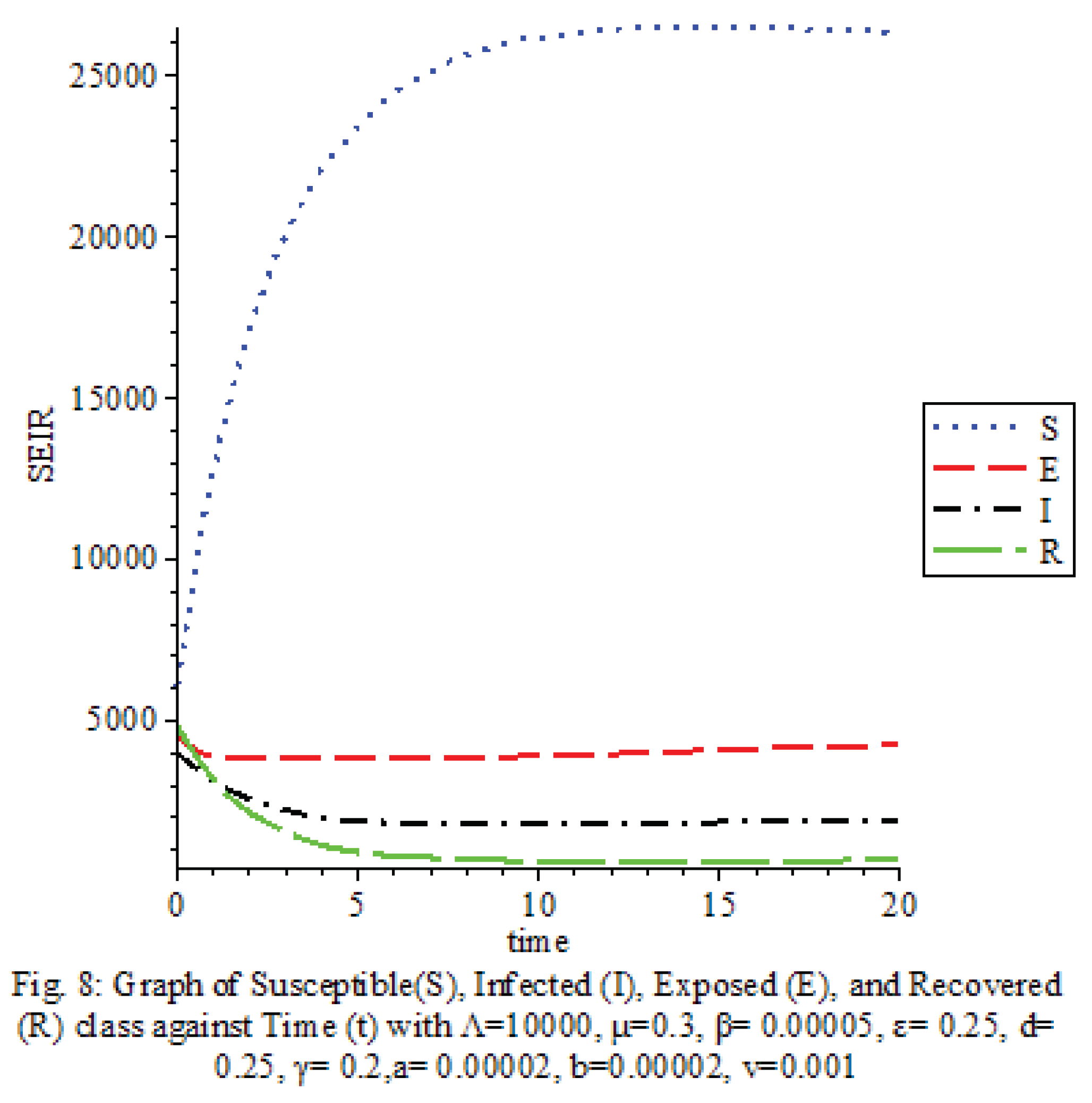
Figure 8 shows that the saturation terms are low

Discussion of Results

The results of our study on the SEIRS COVID-19 pandemic model with saturated incidence rate provide valuable insights into the dynamics of disease transmission and the effectiveness of control measures. Our analysis revealed the significant impact of saturation terms on disease spread, with high saturation terms indicating a more rapid transmission rate compared to low saturation terms. By incorporating vaccine considerations and disease-induced death rates into the model, we were able to assess the role of these factors in controlling the spread of COVID-19.

Furthermore, the examination of the basic reproduction number using the Next Generation Matrix Method allowed us to evaluate the potential for disease control and mitigation strategies. Theorems proving the local and global stabilities of disease-free and endemic equilibria provided a foundation for understanding the dynamics of the pandemic and identifying critical points for intervention. Through numerical simulations, we observed the effects of vaccine coverage, transmission rates, and disease-induced death rates on the model, highlighting the importance of these factors in shaping the trajectory of the pandemic.

Overall, our findings underscore the complexity of COVID-19 transmission dynamics and the need for multifaceted approaches to disease control. By elucidating the interplay of various factors in the spread of the virus, our study contributes to the growing body of knowledge aimed at informing public health policies and interventions to combat the ongoing pandemic.

Conclusion

Our study on the SEIRS COVID-19 pandemic model with saturated incidence rate has provided valuable insights into the dynamics of disease transmission and the impact of key factors such as saturation terms, vaccine coverage, and disease-induced death rates. By analyzing the basic reproduction number and stability of equilibria, we have enhanced our understanding of the spread of COVID-19 and identified critical points for intervention.

It is essential to continue refining and updating mathematical models to reflect the evolving nature of the pandemic and inform evidence-based strategies for disease control. By integrating mathematical modeling with epidemiological insights, we can better navigate the complexities of COVID-19 transmission dynamics and work towards effective public health responses to mitigate the impact of the virus.

References

Olaniyi S and Obabiyi O.S. (2013): Mathematical model for malaria transmission dynamics on human and mosquito population with non-linear forces of infectious disease. Int. Journal of Pure and Applied Mathematics. Vol. 88, pp 125-150.
Jia Li. (2011): Malaria model with stage-structured mosquitoes. Mathematical Biosciences and Engineering. Vol. 8, pp 753-768. [CrossRef]
Agyingi E., Ngwa M. and Wiandt T. (2016): The dynamics of multiple species and strains of malaria. Letters in Biomathematics, vol. 1, pp 29-40.
Kolawole M.K, Olayiwola M.O. (2016): On the numerical simulation of the effect of saturation terms on the SEIRS epidemic model. Allied Research journal; pp 83–90.
Liu W-M, Hethcote HW, Levin SA (1987): Dynamical behavior of epidemiological models with non linear incidence rate. J. Math Biol. vol. 25: pp 359–380.
Van den Driessche P. and Watmough J. (2002): Reproduction numbers and Sub-threshold endemic equilibria for compartmental models of disease transmission. Mathematical Bioscience. vol. 180, pp 29-48. [CrossRef]
Kuniya, Y. Nakata. (2012): Permanence and Extinction for a non-autonomous SEIRS epidemic model. Applied Mathematics and Computations, vol. 218 (18), pp 9321-9331.
Korobeinikov, A. (2004): Lyapunov functions and global properties for SEIR and SEIS epidemic models. Mathematical Medicine and Biology, 21, pp (75-83).
Cai L., Li X., Ghosh M. and Guo B. (2009): Stability analysis of an HIV/AIDS epidemic model with treatment. J. Comput. And Appl. vol. 229, pp313-323.
Kolawole M.K. (2016): Analysis of a SEIRS Epidemic model with saturated incidence rate considering disease induced death. Computing, Information system, Development informatics and Allied Research Journal. vol. 7, No 4, pp 17-28.
WHO. World Health Organization report summary 2020.
Ige, Tosin, William Marfo, Justin Tonkinson, Sikiru Adewale, and Bolanle Hafiz Matti. "Adversarial Sampling for Fairness Testing in Deep Neural Network." arXiv preprint arXiv:2303.02874 (2023). [CrossRef]
Amos Okomayin, Tosin Ige, Abosede Kolade , ” Data Mining in the Context of Legality, Privacy, and Ethics ” International Journal of Research and Scientific Innovation (IJRSI) vol.10 issue 7, pp.10-15 July 2023.
T. Ige and C. Kiekintveld, "Performance Comparison and Implementation of Bayesian Variants for Network Intrusion Detection," 2023 IEEE International Conference on Artificial Intelligence, Blockchain, and Internet of Things (AIBThings), Mount Pleasant, MI, USA, 2023, pp. 1-5. [CrossRef]
Ige, Tosin, and Christopher Kiekintveld. "Performance Comparison and Implementation of Bayesian Variants for Network Intrusion Detection." 2023 IEEE International Conference on Artificial Intelligence, Blockchain, and Internet of Things (AIBThings). IEEE, 2023.
Okomayin, Amos, and Tosin Ige. "Ambient Technology & Intelligence." arXiv preprint arXiv:2305.10726 (2023).
Adewale, Sikiru, Tosin Ige, and Bolanle Hafiz Matti. "Encoder-Decoder Based Long Short-Term Memory (LSTM) Model for Video Captioning." arXiv preprint arXiv:2401.02052 (2023).

Figure 1.

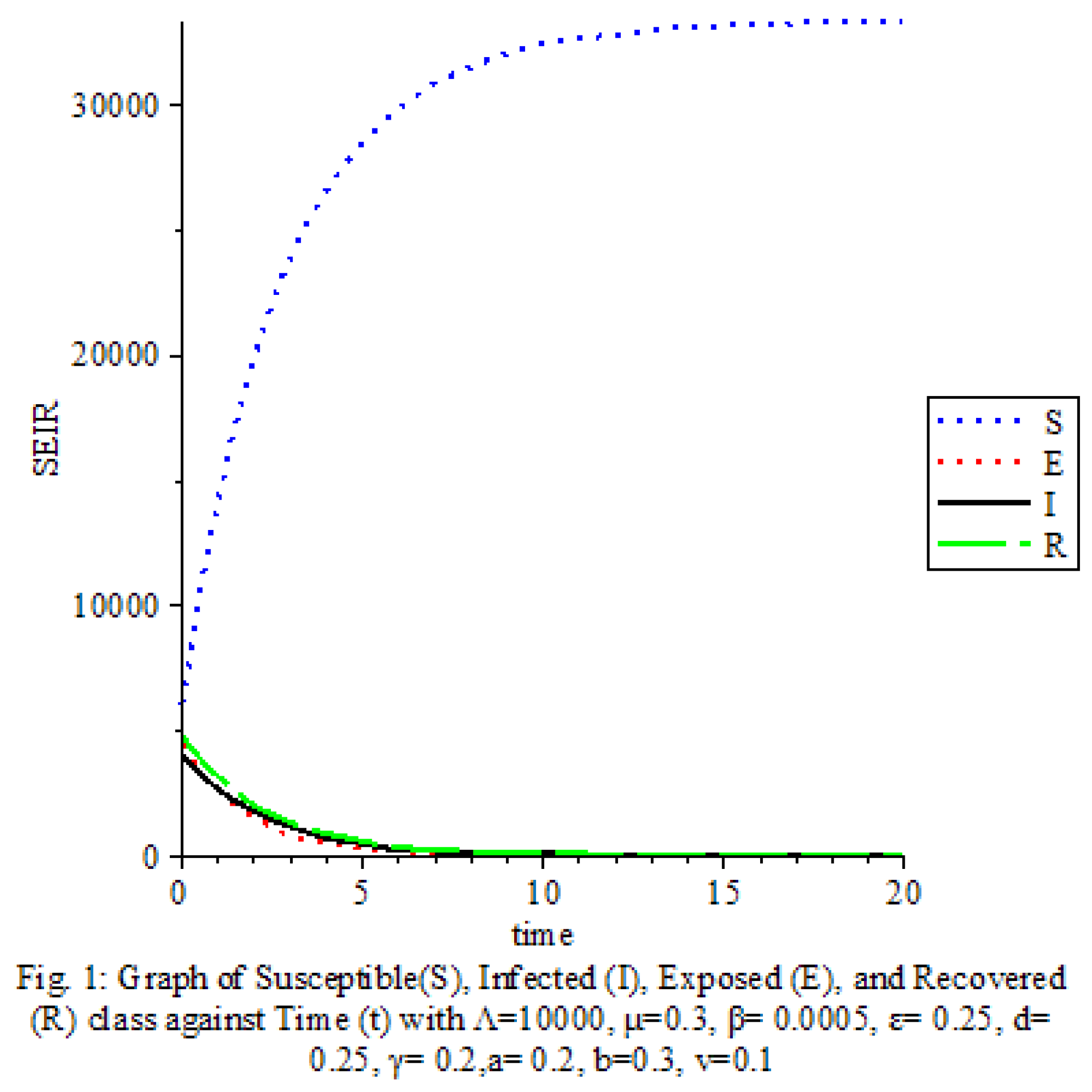
Figure 2.

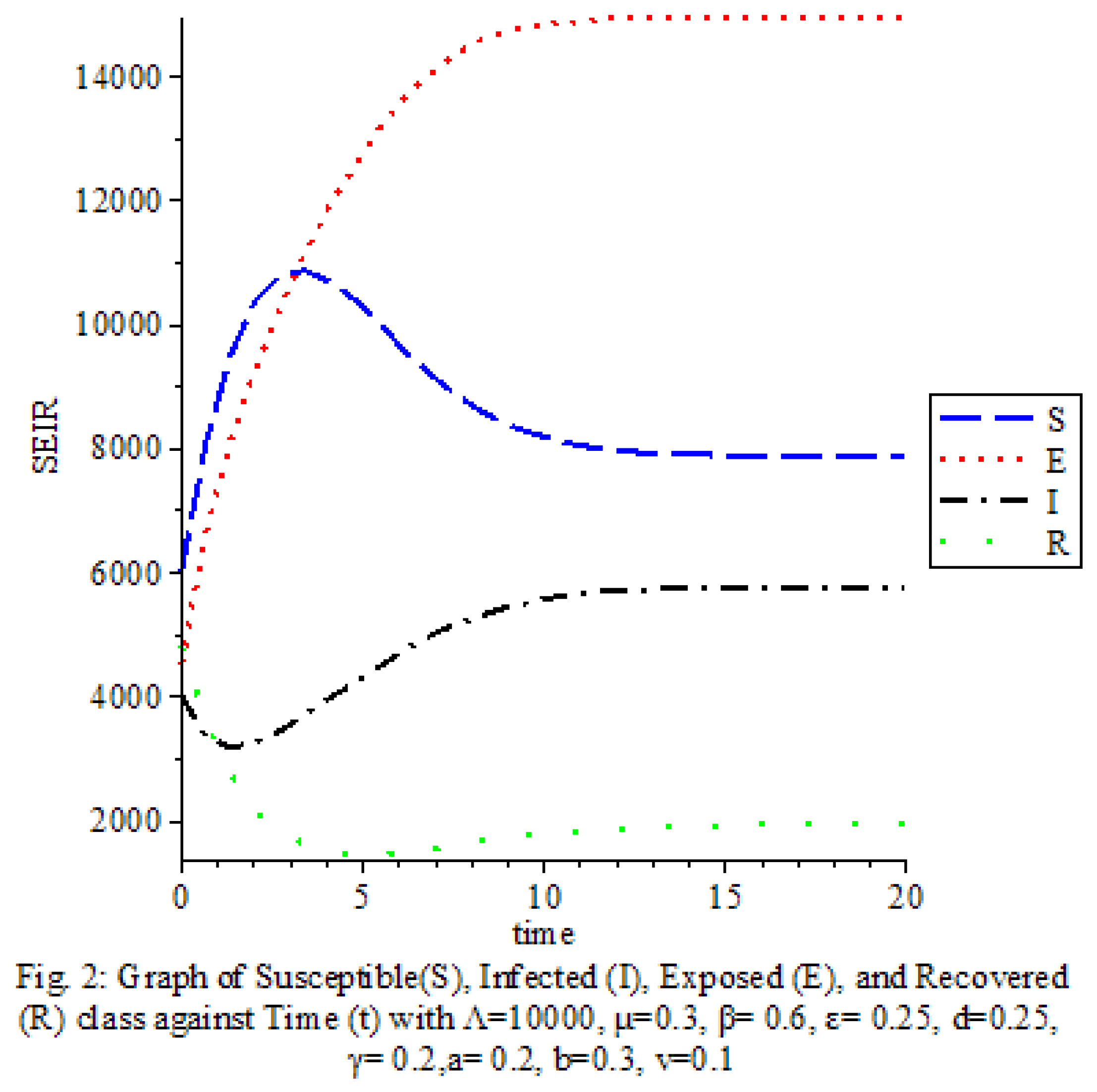
Figure 3.

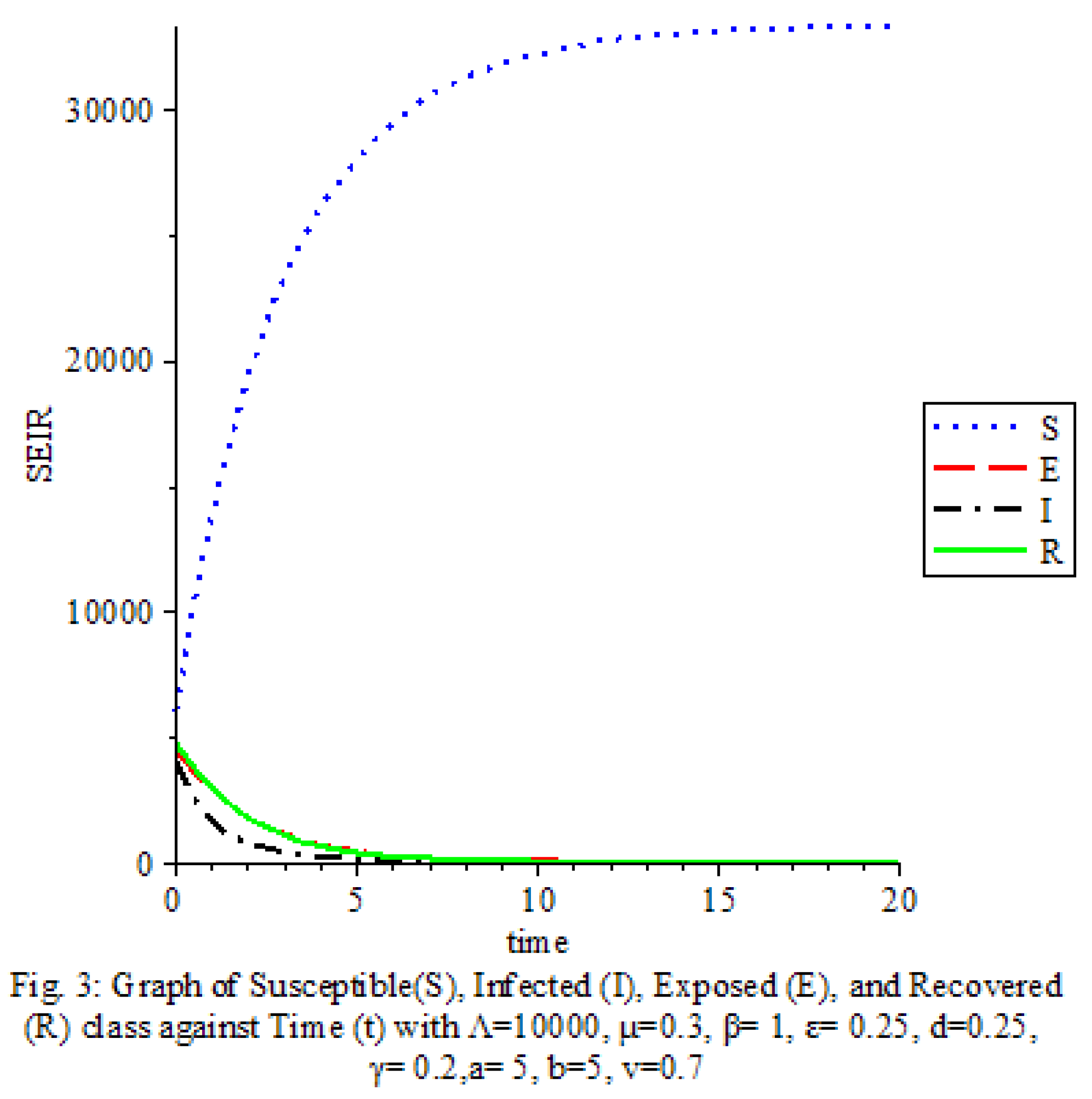
Figure 4.

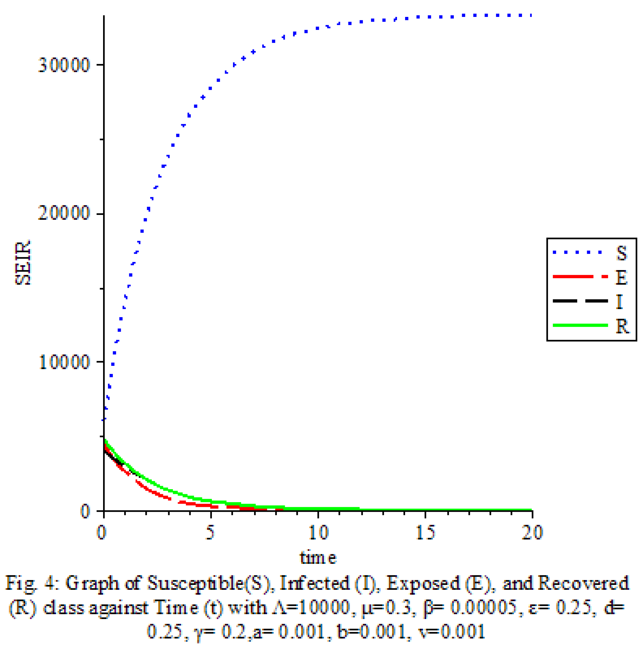
Figure 5.

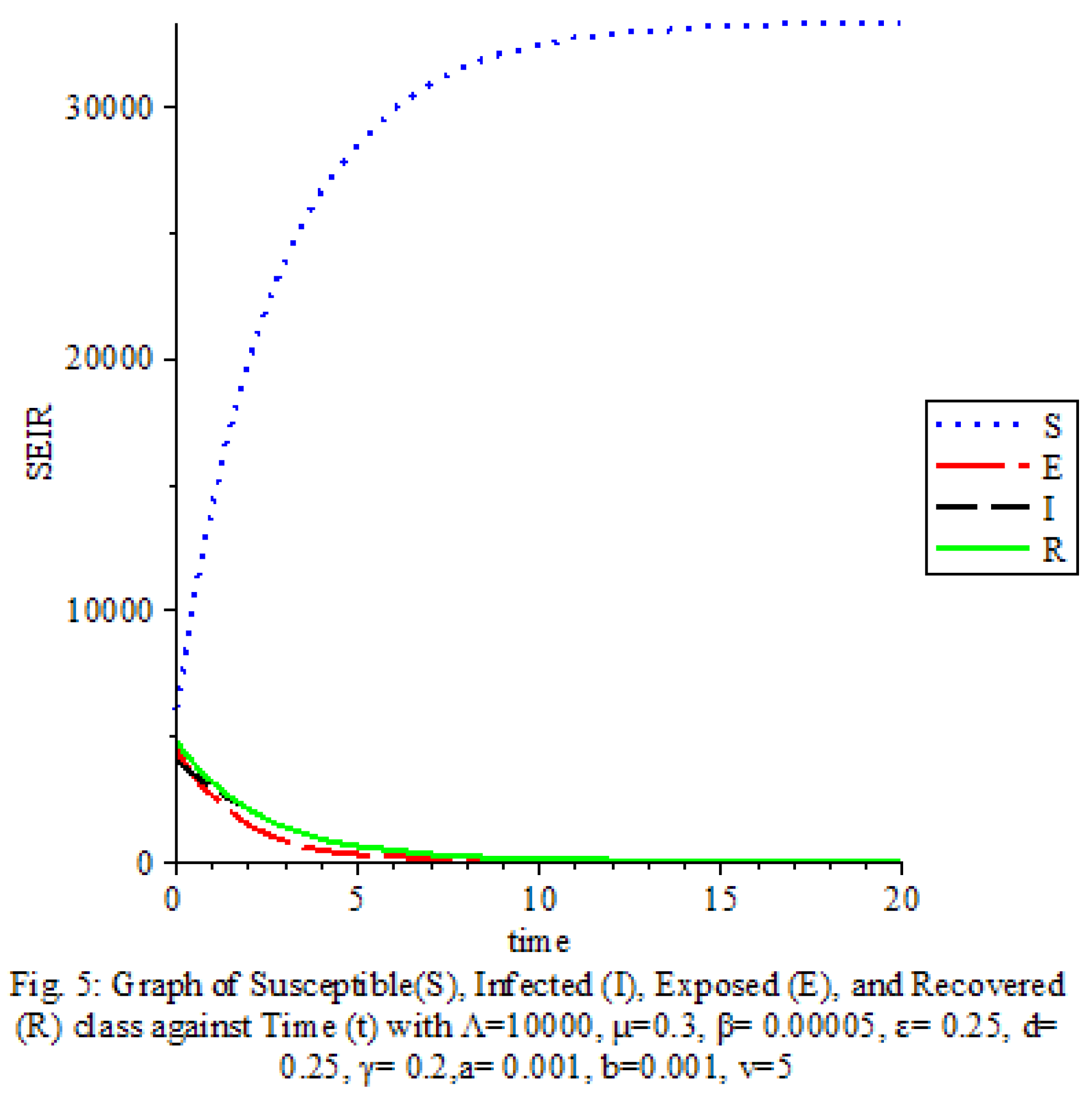
Figure 6.

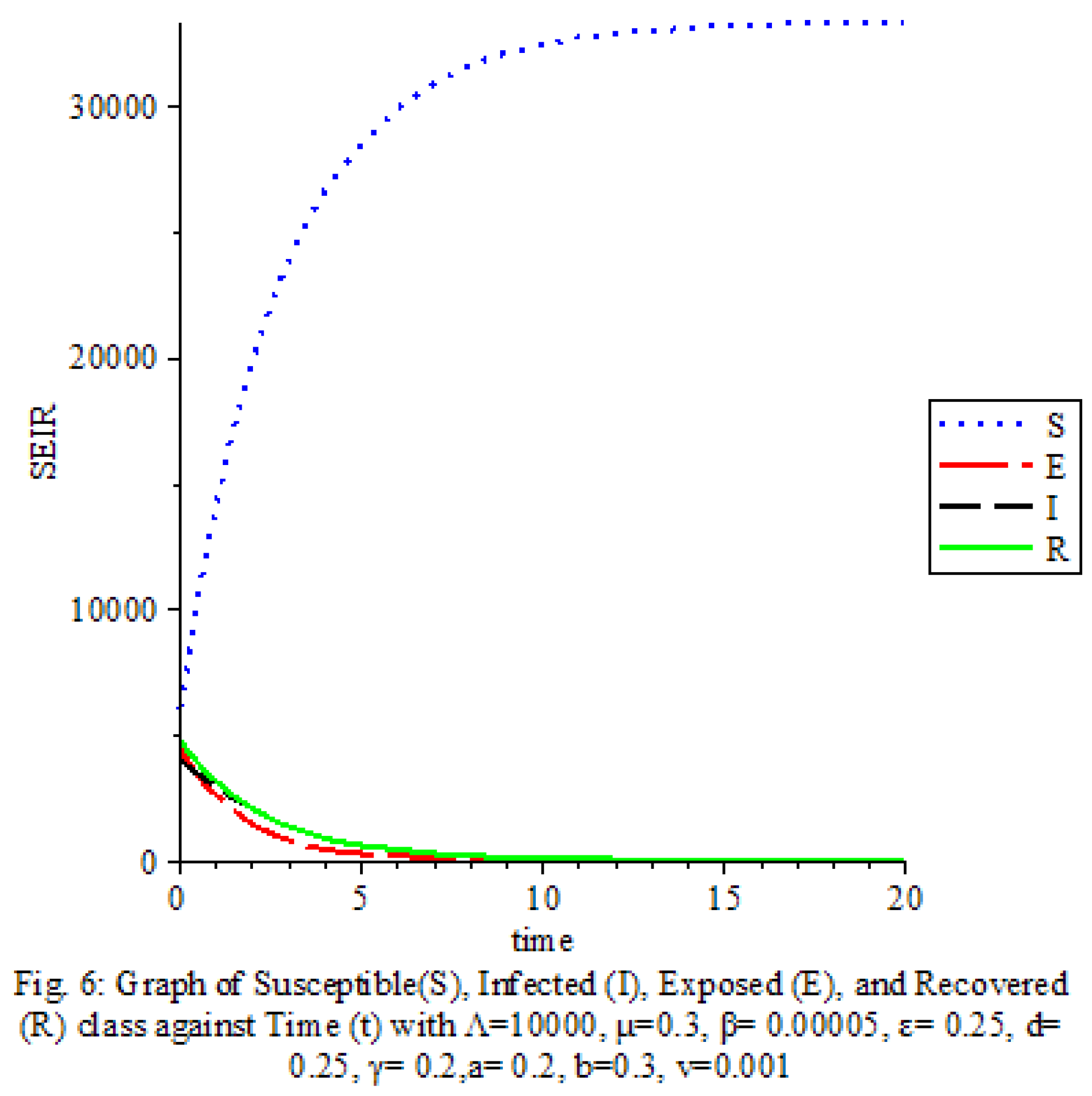
Figure 7.

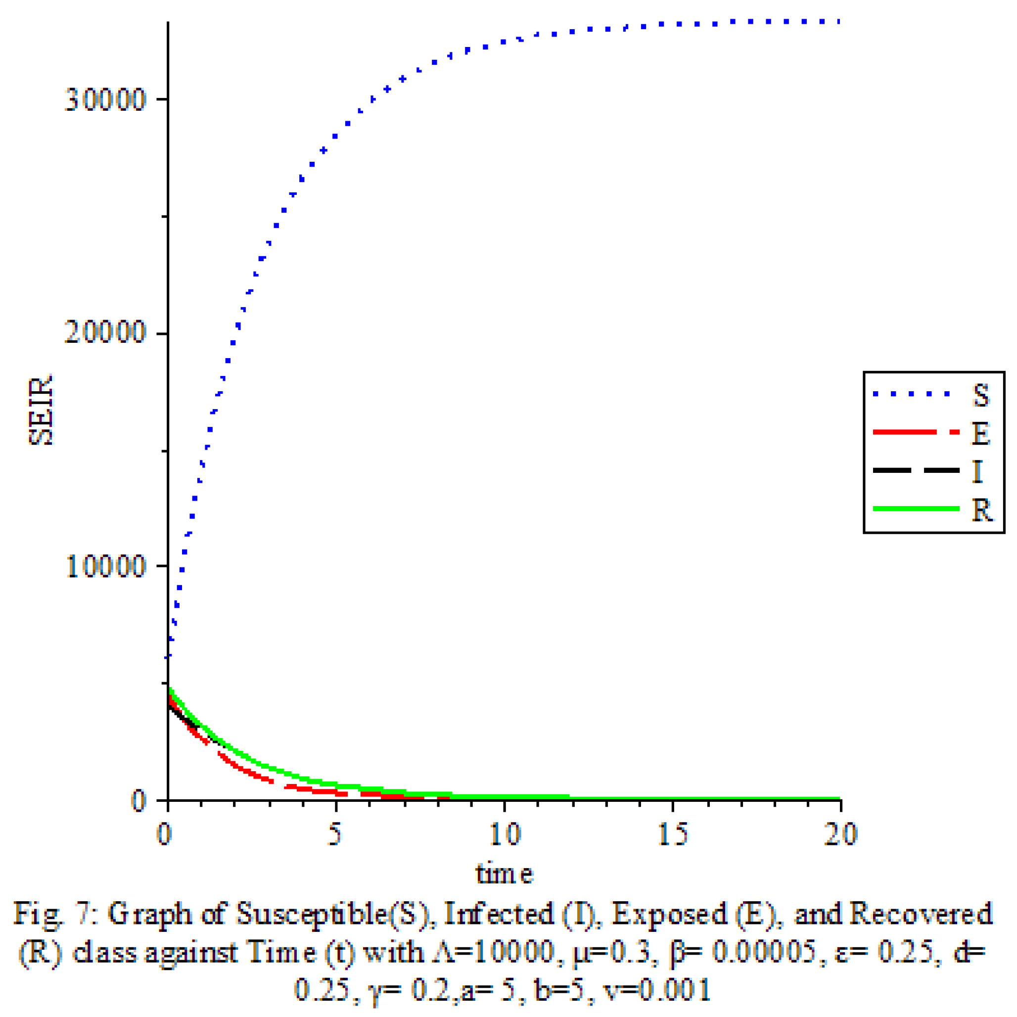
Figure 8.

Disclaimer/Publisher’s Note: The statements, opinions and data contained in all publications are solely those of the individual author(s) and contributor(s) and not of MDPI and/or the editor(s). MDPI and/or the editor(s) disclaim responsibility for any injury to people or property resulting from any ideas, methods, instructions or products referred to in the content.

© 2024 by the authors. Licensee MDPI, Basel, Switzerland. This article is an open access article distributed under the terms and conditions of the Creative Commons Attribution (CC BY) license (http://creativecommons.org/licenses/by/4.0/).

Copyright: This open access article is published under a Creative Commons CC BY 4.0 license, which permit the free download, distribution, and reuse, provided that the author and preprint are cited in any reuse.

Submitted:

05 March 2024

Posted:

05 March 2024

You are already at the latest version

Alerts

Abstract

Keywords:

Subject: Computer Science and Mathematics - Applied Mathematics

Introduction

In this paper, the work of Kolawole M.K. [10] was extended to incorporate vaccine (treatment rate). We present our results in the form of Basic Reproduction Number

R_{0}

2. The Basic Mathematical Model

In this paper, model of Kolawole M.K. (2016) was modified

The Existing model of KOLAWOLE (2016)

\begin{array}{l} \frac{d S}{d t} = \land - \frac{β S I}{1 + m_{1} S + m_{2} I} - μ S + δ R \\ \frac{d E}{d t} = \frac{β S I}{1 + m_{1} S + m_{2} I} - (μ + ε) E \\ \frac{d I}{d t} = ε E - (μ + γ + d) I \\ \frac{d R}{d t} = γ I - (μ + δ) R \end{array}

(1)

Proposed model

\begin{array}{l} \frac{d S}{d t} = \land - \frac{β S I}{1 + m_{1} S + m_{2} I} - μ S + δ R \\ \frac{d E}{d t} = \frac{β S I}{1 + m_{1} S + m_{2} I} - (μ + ε) E \\ \frac{d I}{d t} = ε E - (μ + γ + d + v) I \\ \frac{d R}{d t} = γ I - (μ + δ) R \end{array}

(2)

For the purpose of simplicity, the new Proposed model becomes;

\begin{array}{l} \frac{d S}{d t} = \land - \frac{β S I}{1 + a S + b I} - μ S + δ R \\ \frac{d E}{d t} = \frac{β S I}{1 + a S + b I} - (μ + ε) E \\ \frac{d I}{d t} = ε E - (μ + γ + d + v) I \\ \frac{d R}{d t} = γ I - (μ + δ) R \end{array}

(3)

3. Disease Free Equilibrium (DFE)

At disease free equilibrium

Ι = 0, E = 0, R = 0

\begin{array}{l} \land - \frac{β S I}{1 + a S + b I} - μ S + δ R = 0 \\ \land - μ S = 0 \\ S = \frac{\land}{μ} \\ (S, E, I, R) = (\frac{\land}{μ}, 0, 0, 0) \end{array}

4. Endemic Equilibrium

At Endemic Equilibrium,

I \neq 0,

To get

R^{*}

\begin{array}{l} γ I^{*} - (μ + δ) R^{*} = 0 \\ γ I^{*} = (μ + d) R^{*} \\ R^{*} = \frac{γ I^{*}}{μ + δ} \end{array}

(4)

Then

S^{*}

gives,

\begin{array}{l} \frac{β S^{*} I^{*}}{1 + a S^{*} + b I^{*}} - (μ + ε) E^{*} = 0 \\ \frac{β S^{*} I^{*}}{1 + a S^{*} + b I^{*}} = (μ + ε) E^{*} \\ β S^{*} I^{*} = (1 + a S^{*} + b I^{*}) (μ + ε) E^{*} \\ β S^{*} I^{*} = a S^{*} (μ + ε) E^{*} + (1 + b I^{*}) (μ + ε) E^{*} \\ β S^{*} I^{*} - a S^{*} (μ + ε) E^{*} = (1 + b I^{*}) (μ + ε) E^{*} \\ S^{*} = \frac{(1 + b I^{*}) (μ + ε) E^{*}}{β I^{*} - a (μ + ε) E^{*}} \end{array}

(5)

Then compartment

I^{*}

becomes,

\begin{array}{l} \land - \frac{β S^{*} I^{*}}{1 + a S^{*} + b I^{*}} - μ S^{*} + δ R^{*} = 0 \\ \land - μ S^{*} + δ R^{*} = \frac{β S^{*} I^{*}}{1 + a S^{*} + b I^{*}} \\ (\land - μ S^{*} + δ R^{*}) (1 + a S^{*} + b I^{*}) = β S^{*} I^{*} \\ (\land - μ S^{*} + δ R^{*}) (1 + a S^{*}) + (\land - μ S^{*} + δ R) b I^{*} = β S^{*} I^{*} \\ (\land - μ S^{*} + δ R^{*}) (1 + a S^{*}) = β S^{*} I^{*} - (\land - μ S^{*} + δ R) b I^{*} \\ I^{*} = \frac{(\land - μ S^{*} + δ R^{*}) (1 + a S^{*})}{β S^{*} - b (\land - μ S^{*} + δ R^{*})} \end{array}

(6)

Then

E^{*}

becomes,

\begin{array}{l} \begin{array}{l} ε E^{*} - (μ + γ + d + v) I^{*} = 0 \\ ε E^{*} = (μ + γ + d + v) I^{*} \end{array} \\ E^{*} = \frac{(d + α + m) I^{*}}{ε} \end{array}

(7)

5. Basic Reproduction Number $R_{0}$

Using next generation matrix,

R_{0} = F \times V^{- 1}

F = [\begin{matrix} \frac{β \land}{μ + a \land} & 0 \\ 0 & 0 \end{matrix}] and V = [\begin{matrix} 0 & (μ + ε) \\ (μ + γ + d + v) & - ε \end{matrix}]

The inverse of

V

is obtained as

V^{- 1} = \frac{- 1}{(μ + ε) (μ + γ + d + v)} [\begin{matrix} - ε & (μ + ε) \\ (μ + γ + d + v) & 0 \end{matrix}]

Hence,

\begin{array}{l} R_{0} = F . V^{- 1} = [\begin{matrix} \frac{β \land}{μ + a \land} & 0 \\ 0 & 0 \end{matrix}] [\begin{matrix} \frac{ε}{(μ + ε) (μ + γ + d + v)} & \frac{- 1}{(μ + γ + d + v)} \\ \frac{- 1}{(μ + ε)} & 0 \end{matrix}] \\ R_{0} = [\begin{matrix} \frac{β \land ε}{(μ + a \land) (μ + ε) (μ + γ + d + v)} & 0 \\ 0 & 0 \end{matrix}] \end{array}

The equation with the dominant Eigen value becomes,

R_{0} = \frac{β \land ε}{(μ + a \land) (μ + ε) (μ + γ + d + v)}

(8)

6. Local Stability of Disease Free Equilibrium

We Linearize the system of equation in (3) by setting

\begin{array}{l} S - S_{1} = x, E = E, I = I, R = R \\ S = x + S_{1} \end{array}

Where

S_{1} = \frac{\land}{μ}

Therefore,

\begin{array}{l} \frac{d S}{d t} = \land - \frac{β S I}{1 + a S + b I} - μ S + δ R \\ \frac{d E}{d t} = \frac{β S I}{1 + a S + b I} - (μ + ε) E \\ \frac{d I}{d t} = ε E - (μ + γ + d + v) I \\ \frac{d R}{d t} = γ I - (μ + δ) R \end{array}

(9)

The Linearized system gives,

\begin{array}{l} \frac{d x}{d t} = - μ x + \frac{β \land}{μ} (\frac{a \land}{μ} - 1) I + Non linear terms \\ \frac{d E}{d t} = \frac{β \land}{μ} (1 - \frac{a \land}{μ}) I - (μ + ε) E + Non linear terms \\ \frac{d I}{d t} = ε E - (μ + γ + d + v) I + Non linear terms \\ \frac{d R}{d t} = γ I - (μ + δ) R + Non linear terms \end{array}

(10)

The Jacobian matrix of equation (10) becomes,

J (E_{0}) = [\begin{matrix} - μ & 0 & \frac{β \land}{μ} (\frac{a \land}{μ} - 1) & δ \\ 0 & - (μ + ε) & \frac{β \land}{μ} (1 - \frac{a \land}{μ}) & 0 \\ 0 & ε & - (μ + γ + d + v) & 0 \\ 0 & 0 & γ & - (μ + δ) \end{matrix}]

Then the determinant

|A - I λ| = 0

becomes,

J (E_{0}) = |\begin{matrix} - μ & 0 & \frac{β \land}{μ} (\frac{a \land}{μ} - 1) & δ \\ 0 & - (μ + ε) & \frac{β \land}{μ} (1 - \frac{a \land}{μ}) & 0 \\ 0 & ε & - (μ + γ + d + v) & 0 \\ 0 & 0 & γ & - (μ + δ) \end{matrix}| = 0

(11)

The solutions give,

λ_{1} = - μ λ_{2} = - (μ + δ)

λ_{3} = \frac{1}{μ} (- \frac{1}{2} μ d - \frac{1}{2} μ ε - \frac{1}{2} μ γ - μ^{2} - \frac{1}{2} μ v + \frac{1}{2} \sqrt{D})

λ_{3} = \frac{1}{μ} (- \frac{1}{2} μ d - \frac{1}{2} μ ε - \frac{1}{2} μ γ - μ^{2} - \frac{1}{2} μ v + \frac{1}{2} \sqrt{D})

Where

D = \sqrt{- 4 \land^{2} a β ε + 4 \land β ε μ + d^{2} μ^{2} - 2 d ε μ^{2} + 2 d γ μ^{2} + 2 d μ^{2} v + ε^{2} μ^{2} - 2 ε γ μ^{2} - 2 ε μ^{2} v + γ^{2} μ^{2} + 2 γ μ^{2} v + μ^{2} v^{2}}

Theorem:

R_{0} < \frac{μ^{2}}{μ^{2} - \land^{2} a^{2}} < 1,

therefore, the disease free equilibrium is Locally asymptotically Stable and if

R_{0} > \frac{μ^{2}}{μ^{2} - \land^{2} a^{2}} > 1,

therefore the disease equilibrium is unstable.

Proof:

The characteristic equation from equation (11) gives

λ_{1} = - μ λ_{2} = - (μ + δ)

λ_{1} = - μ λ^{2} + (2 μ + ε + γ + d + v) λ + (μ + ε) (μ + γ + d + v) (1 - (\frac{μ^{2} - \land^{2} a^{2}}{μ^{2}}) R_{0}) = 0

(12)

By Descartes rule of signs, it shows that there are no signs changes in equation (12), If

R_{0} < \frac{μ^{2}}{μ^{2} - \land^{2} a^{2}} < 1,

Implies that there are no positive root in equation (12). Now, if

λ

is replaced with

- λ

in equation (12), we have

λ^{2} - (2 μ + ε + γ + d + v) λ + (μ + ε) (μ + γ + d + v) (1 - (\frac{μ^{2} - \land^{2} a^{2}}{μ^{2}}) R_{0}) = 0

(13)

There are two sign changes in the above equilibrium; hence it has two exact negative roots of

R_{0} < \frac{μ^{2}}{μ^{2} - \land^{2} a^{2}} < 1,

Hence, the Eigen values of equation (13) are all negative i.e.

λ_{3} = \frac{1}{μ} (- \frac{1}{2} μ d - \frac{1}{2} μ ε - \frac{1}{2} μ γ - μ^{2} - \frac{1}{2} μ v + \frac{1}{2} \sqrt{D})

λ_{4} = \frac{1}{μ} (- \frac{1}{2} μ d - \frac{1}{2} μ ε - \frac{1}{2} μ γ - μ^{2} - \frac{1}{2} μ v - \frac{1}{2} \sqrt{D})

Since

λ_{1}, λ_{2}, λ_{3} a n d λ_{4}

are all negative, it follows that the disease free equilibrium is Locally Asymptotically stable.

Now, if

R_{0} > \frac{μ^{2}}{μ^{2} - \land^{2} a^{2}} > 1,

in equation (12) then,

It shows that only one sign will be positive then the other part will be negative.

Now, if

λ

is replaced with

- λ

in equation (13), we say

λ^{2} + (2 μ + ε + γ + d + v) λ - (μ + ε) (μ + γ + d + v) (1 - (\frac{μ^{2} - \land^{2} a^{2}}{μ^{2}}) R_{0}) = 0

(14)

There are one sign changes in the above equilibrium; hence it has one exact negative root. Also, we replace

λ

w i t h ​ - λ w e h a v e

λ^{2} - (2 μ + ε + γ + d + v) λ + (μ + ε) (μ + γ + d + v) (1 - (\frac{μ^{2} - \land^{2} a^{2}}{μ^{2}}) R_{0}) = 0

(15)

There is just a sign change, which shows that there is one negative root. That is, not all Eigen Values are negative, hence the disease free equilibrium point

(S, E, I, R) = (\frac{\land}{μ}, 0, 0, 0)

is unstable If

R_{0} > \frac{μ^{2}}{μ^{2} - \land^{2} a^{2}} > 1.

7. Global Stability of Disease Free Equilibrium

We consider the Lyapunov function,

\begin{array}{l} V = ε E^{'} + (μ + ε) I^{'} (16) \\ \frac{d V}{d t} = ε \frac{d E}{d t} + (μ + ε) \frac{d I}{d t} \end{array}

(16)

At disease free equilibrium, we have

(S, E, I, R) = (\frac{\land}{μ}, 0, 0, 0)

Then we have,

\begin{array}{l} \frac{d V}{d t} = μ [\frac{β S I}{1 + a S + b I} - (μ + ε) E] + (d + μ) [ε E - (μ + γ + d + v) I] \\ \frac{d v}{d t} = (μ + ε) (μ + γ + d + v) [\frac{β \land ε}{(μ + a \land) (μ + ε) (μ + γ + d + v)} - 1] I \end{array}

\begin{array}{l} \frac{d V}{d t} = μ [\frac{β S I}{1 + a S + b I} - (μ + ε) E] + (d + μ) [ε E - (μ + γ + d + v) I] \\ \frac{d v}{d t} = (μ + ε) (μ + γ + d + v) [\frac{β \land ε}{(μ + a \land) (μ + ε) (μ + γ + d + v)} - 1] I \\ L^{1} = (μ + ε) (μ + γ + d + v) [R_{0} - 1] \leq 0 \\ I f R_{0} \leq 1 \\ L^{1} \leq 0 \end{array}

(17)

Hence, the Disease Free Equilibrium is Globally Asymptotically Stable.

8. Local Stability of Endemic Equilibrium

Let

\begin{array}{l} S - S^{*} = w, E - E^{*} = x, I - I^{*} = y, R - R^{*} = z \\ \frac{d s}{d t} = \frac{d w}{d t}, \frac{d E}{d t} = \frac{d x}{d t}, \frac{d I}{d t} = \frac{d y}{d t}, \frac{d R}{d t} = \frac{d z}{d t} \end{array}

Then, we have

\begin{array}{l} \frac{d w}{d t} = (- β I^{*} + 2 β I^{*} a S^{*} + β I^{*^{2}} b - μ) w + (- β S^{*} + β S^{*} a + 2 β S^{*} b I^{*}) y + δ z + non linear terms \\ \frac{d x}{d t} = (β I^{*} - 2 β I^{*} a S^{*} - {β I^{*}}^{2} b) w + (β S^{*} - β S^{*} a - 2 β S^{*} b I^{*}) y - (μ + ε) x + non linear terms \\ \frac{dy}{dt} = ε x - (μ + γ + d + v) y + non linear terms \\ \frac{dz}{dt} = γ y - (μ + δ) z + non linear terms \end{array}

(18)

The Jacobian Matrix in (18) becomes,

(\dot{\begin{array}{l} w \\ \dot{\begin{array}{l} x \\ \dot{\begin{array}{l} y \\ \dot{z} \end{array}} \end{array}} \end{array}}) = (\begin{matrix} (- β I^{*} + 2 β I^{*} a S^{*} + β I^{*^{2}} b - μ) & 0 & (- β S^{*} + β S^{*} a + 2 β S^{*} b I^{*}) & δ \\ (β I^{*} - 2 β I^{*} a S^{*} - {β I^{*}}^{2} b) & - (μ + ε) & (β S^{*} - β S^{*} a - 2 β S^{*} b I^{*}) & 0 \\ 0 & ε & - (μ + γ + d + v) & 0 \\ 0 & 0 & γ & - (μ + δ) \end{matrix}) (\begin{array}{l} w \\ x \\ y \\ z \end{array}) + Non Linear terms

(19)

Also, the characteristic equation

|A^{*} - I λ| = 0

gives,

|A^{*} - I λ| = |\begin{matrix} (- β I^{*} + 2 β I^{*} a S^{*} + β I^{*^{2}} b - μ) - λ & 0 & (- β S^{*} + β S^{*} a + 2 β S^{*} b I^{*}) & δ \\ (β I^{*} - 2 β I^{*} a S^{*} - {β I^{*}}^{2} b) & - (μ + ε) - λ & (β S^{*} - β S^{*} a - 2 β S^{*} b I^{*}) & 0 \\ 0 & ε & - (μ + γ + d + v) - λ & 0 \\ 0 & 0 & γ & - (μ + δ) - λ \end{matrix}| = 0

(20)

Let

\begin{array}{l} P_{0} = - β I^{*} + 2 β I^{*} a S^{*} + β I^{*^{2}} b - μ \\ P_{1} = - β S^{*} + β S^{*} a + 2 β S^{*} b I^{*} \\ P_{2} = β I^{*} - 2 β I^{*} a S^{*} - {β I^{*}}^{2} b \\ P_{3} = β S^{*} - β S^{*} a - 2 β S^{*} b I^{*} \end{array}

Now, we have

|A^{*} - I λ| = |\begin{matrix} P_{0} - λ & 0 & P_{1} & δ \\ P_{2} & - (μ + ε) - λ & P_{3} & 0 \\ 0 & ε & - (μ + γ + d + v) - λ & 0 \\ 0 & 0 & γ & - (μ + δ) - λ \end{matrix}| = 0

(21)

Hence,

By Descartes rule of sign, we say

\begin{array}{l} P_{4} = - P_{0} + d + δ + ε + γ + 3 μ + v \\ P_{5} = - (d + δ + ε + γ + v) P_{0} - P_{3} ε + d δ + 2 δ ε + 2 d + δ γ + 2 δ μ + δ v + ε γ + 2 ε μ + ε v + 2 γ μ + 3 μ^{2} + 2 μ v \\ P_{6} = (P_{3} ε - d δ - d ε - 2 d μ - δ ε - δ γ - 2 δ μ - δ v - ε γ - 2 ε μ - ε v - 2 γ μ - 3 μ^{2} - 2 μ v) P_{0} - P_{1} P_{2} ε - P_{3} δ ε \\ - P_{3} ε μ + d δ ε + d δ μ + 2 d ε μ + d μ^{2} + δ ε γ + δ ε v + δ γ μ + δ μ^{2} + δ μ v + ε γ μ + ε μ^{2} + ε μ v + γ μ^{2} + μ^{3} + μ^{2} v) \\ P_{7} = P_{0} P_{3} δ ε + P_{0} P_{3} ε μ - P_{0} d δ ε - P_{0} d δ μ - P_{0} d ε μ - P_{0} d μ^{2} - P_{0} δ ε γ - P_{0} δ ε μ - P_{0} δ ε v - P_{0} δ γ μ - P_{0} δ μ^{2} - P_{0} δ μ v \\ - P_{0} ε γ μ - P_{0} ε μ^{2} - P_{0} ε μ v - P_{0} γ μ^{2} - P_{0} μ^{3} - P_{0} μ^{2} v - P_{1} P_{2} δ ε - P_{1} P_{2} ε μ - P_{2} ε γ δ \end{array}

(22)

Equation (22) gives

f (λ) = λ^{4} - P_{4} λ^{3} - P_{5} λ^{2} - P_{6} λ - P_{7} = 0

(23)

Let

P_{4} < 0, P_{5} < 0, P_{6} < 0, P_{7} < 0

in (22), and then

f (λ)

have no change in sign meaning there are no positive roots of

f (λ)

Also, if we replace

λ

- λ

in (23), gives

f (- λ) = λ^{4} + P_{4} λ^{3} - P_{5} λ^{2} - P_{6} λ - P_{7} = 0

(24)

P_{4} < 0, P_{5} < 0, P_{6} < 0, P_{7} < 0

in (25) have 4 sign changes, which implies that there are exactly 4 negative roots of

f (- λ)

. Since there are no positive roots for

P_{4} < 0, P_{5} < 0, P_{6} < 0, P_{7} < 0

Therefore, it implies that since all Eigen values are negative the endemic equilibrium is Locally Asymptotically Stable.

9. Results and Discussion

Figure 1 shows that the transmission rate is low.

Figure 2 shows that the transmission rate is high

Figure 3 shows that the transmission rate, Saturation terms and Vaccine are high

Figure 4 shows that the transmission rate, Saturation terms and Vaccine are low

Figure 5 shows that the Vaccine is high

Figure 6 shows that Vaccine is low

Figure 7 shows that the saturation terms are high

Figure 8 shows that the saturation terms are low

Discussion of Results

Conclusion

References

Olaniyi S and Obabiyi O.S. (2013): Mathematical model for malaria transmission dynamics on human and mosquito population with non-linear forces of infectious disease. Int. Journal of Pure and Applied Mathematics. Vol. 88, pp 125-150.
Jia Li. (2011): Malaria model with stage-structured mosquitoes. Mathematical Biosciences and Engineering. Vol. 8, pp 753-768. [CrossRef]
Agyingi E., Ngwa M. and Wiandt T. (2016): The dynamics of multiple species and strains of malaria. Letters in Biomathematics, vol. 1, pp 29-40.
Kolawole M.K, Olayiwola M.O. (2016): On the numerical simulation of the effect of saturation terms on the SEIRS epidemic model. Allied Research journal; pp 83–90.
Liu W-M, Hethcote HW, Levin SA (1987): Dynamical behavior of epidemiological models with non linear incidence rate. J. Math Biol. vol. 25: pp 359–380.
Van den Driessche P. and Watmough J. (2002): Reproduction numbers and Sub-threshold endemic equilibria for compartmental models of disease transmission. Mathematical Bioscience. vol. 180, pp 29-48. [CrossRef]
Kuniya, Y. Nakata. (2012): Permanence and Extinction for a non-autonomous SEIRS epidemic model. Applied Mathematics and Computations, vol. 218 (18), pp 9321-9331.
Korobeinikov, A. (2004): Lyapunov functions and global properties for SEIR and SEIS epidemic models. Mathematical Medicine and Biology, 21, pp (75-83).
Cai L., Li X., Ghosh M. and Guo B. (2009): Stability analysis of an HIV/AIDS epidemic model with treatment. J. Comput. And Appl. vol. 229, pp313-323.
Kolawole M.K. (2016): Analysis of a SEIRS Epidemic model with saturated incidence rate considering disease induced death. Computing, Information system, Development informatics and Allied Research Journal. vol. 7, No 4, pp 17-28.
WHO. World Health Organization report summary 2020.
Ige, Tosin, William Marfo, Justin Tonkinson, Sikiru Adewale, and Bolanle Hafiz Matti. "Adversarial Sampling for Fairness Testing in Deep Neural Network." arXiv preprint arXiv:2303.02874 (2023). [CrossRef]
Amos Okomayin, Tosin Ige, Abosede Kolade , ” Data Mining in the Context of Legality, Privacy, and Ethics ” International Journal of Research and Scientific Innovation (IJRSI) vol.10 issue 7, pp.10-15 July 2023.
T. Ige and C. Kiekintveld, "Performance Comparison and Implementation of Bayesian Variants for Network Intrusion Detection," 2023 IEEE International Conference on Artificial Intelligence, Blockchain, and Internet of Things (AIBThings), Mount Pleasant, MI, USA, 2023, pp. 1-5. [CrossRef]
Ige, Tosin, and Christopher Kiekintveld. "Performance Comparison and Implementation of Bayesian Variants for Network Intrusion Detection." 2023 IEEE International Conference on Artificial Intelligence, Blockchain, and Internet of Things (AIBThings). IEEE, 2023.
Okomayin, Amos, and Tosin Ige. "Ambient Technology & Intelligence." arXiv preprint arXiv:2305.10726 (2023).
Adewale, Sikiru, Tosin Ige, and Bolanle Hafiz Matti. "Encoder-Decoder Based Long Short-Term Memory (LSTM) Model for Video Captioning." arXiv preprint arXiv:2401.02052 (2023).

Figure 1.

Figure 2.

Figure 3.

Figure 4.

Figure 5.

Figure 6.

Figure 7.

Figure 8.

MDPI Initiatives

Important Links

Choose an area of interest and we will send you notifications of new preprints at your preferred frequency.

Disclaimer

Modeling Pandemic Vaccine with Saturated Incidence Rate Based on Disease Induced Death

Abstract

Introduction

2. The Basic Mathematical Model

3. Disease Free Equilibrium (DFE)

4. Endemic Equilibrium

5. Basic Reproduction Number R 0

6. Local Stability of Disease Free Equilibrium

7. Global Stability of Disease Free Equilibrium

8. Local Stability of Endemic Equilibrium

9. Results and Discussion

Discussion of Results

Conclusion

References

Abstract

Introduction

2. The Basic Mathematical Model

3. Disease Free Equilibrium (DFE)

4. Endemic Equilibrium

5. Basic Reproduction Number R 0

6. Local Stability of Disease Free Equilibrium

7. Global Stability of Disease Free Equilibrium

8. Local Stability of Endemic Equilibrium

9. Results and Discussion

Discussion of Results

Conclusion

References

MDPI Initiatives

Important Links

Subscribe

5. Basic Reproduction Number $R_{0}$

5. Basic Reproduction Number $R_{0}$