1. Introduction
The demand for water is on the rise due to population expansion, intensified agriculture, urbanization, and industrial growth [
1,
2,
3]. Both human activities and natural sources of pollution pose threats to water resources, surpassing their suitability for drinking, irrigation, industrial, and other essential purposes [
4,
5]. The use of reclaimed water (RW) for irrigation is a common practice globally, even in the regions with plenty of available water resources [
6,
7]. Utilizing treated wastewater is seen as one of the ways to use it for irrigation purposes [
8] since it requires less-clean water, depending on the crop type and how much contact people have with it. Moreover, using reclaimed wastewater for irrigation helps by providing nutrients that reduce the need for fertilizers. However, whether this happens a lot or not, it mostly relies on the government regulations and how society accept its use which can differ between countries and communities [
9]. Using wastewater for agriculture, especially in dry, low-income areas, has proven to be a cost-effective and dependable water source. Wastewater carries nitrogen and phosphorus that can enhance crop yields. Studies reveal that using wastewater is cheaper than irrigating with canal water, even though it demands more frequent and intensive labor. Various investigations across Asia, West Africa, and Latin America highlight its benefits. For instance, in Pakistan and Ghana, farmers generate significant income and profits by irrigating with wastewater. In India and Zimbabwe, estimates show substantial nutrient values in wastewater that, if managed well, could reduce the need for chemical fertilizers to a greater extent in farming. However, while urban agriculture using wastewater can provide short-term benefits, there are concerns regarding health and environmental implications that need attention [
10].
To limit the public health concerns linked with the use of wastewater for irrigation, the WHO in its guidelines published in 1973, 1989, and 2006 have addressed the safe practices for the utilization of treated waste water in irrigation [
11,
12,
13]. Supporting similar initiates, the FAO also recommended two guidelines. The initial FAO guideline emphasizes on the potential issues for crop cultivation by classifying irrigation water according to variables such sodicity, salinity, toxicity, and other hazards [
14]. In its second guideline, it further focused at the water reuse in irrigation while considering various groupings according to the kind of crops that are irrigated [
15]. Additionally, the EPA support the previously published guidelines while prioritizing the environmental preservation and the public health. Thus, serving as a reliable reference responsible for the wastewater reuse [
16,
17].
To assess the suitability of treated wastewater for irrigation, electrical conductivity (EC) is said to be one of the important parameters [
18], since it reflects the risk of soil salinity which could adversely affect the crop yield and its productivity. Basically, the higher EC values of the water could lead to the possibility of physiological drought where the plants cannot compete with the ions in the soil solution for water. Thus, for most of the crops, it has been stated that the water used for irrigation should have an EC value in the range of 750–2250 μS/cm. In case, if the water contains higher EC values then the salinity management practices like adequate drainage and leaching should be properly implemented [
19]. Moreover, some ions including calcium, sodium and magnesium could affect the sodium absorption ratio (SAR), another crucial factor for assessing the sodicity risk of groundwater for irrigation [
20]. Previous studies have demonstrated that treated wastewater’s average EC values can differ significantly. For instance, one of the studies reported EC values ranging from 781 to 2810 µS/cm, with a mean value of 1801.7 µS/cm [
19]. Another study indicated that EC values in groundwater varied from 63 to 3819 µS/cm, with the majority of wells consisting of freshwater (< 1000 µS/cm) during rainy seasons [
21]. It has been stressed that in order to assure sustainable agricultural activities, the treated wastewater should meet the given quality standards by involving a close monitoring just not on the EC but also at the other variables including pH, TDS, BOD, COD, nutrient contents, etc. [
19].
It is imperative to predict the dynamics of the soil salinization for ecosystem preservation, agricultural management, and sustainable irrigation management [
22]. One of the studies projected soil salinity variations under the climate change effects in the Khorezm area of Uzbekistan by an ex-ante analysis using a statistical framework. The study outcomes showed a decline in mildly salty soils but an increase in moderately and extremely saline soils. This highlighted that how crucial it is to comprehend how the climate affects soil salinity dynamics in order to implement appropriate regional management [
23]. Consequently, the use of digital soil mapping and machine learning (ML) approach adopted by Taghizadeh-Mehrjardi et al., 2021, utilized the W-SVR (wavelet transformation with support vector regression) approach. Despite a greater correlation coefficient, the W-SVR outperformed other proposed models, particularly when predicting soil salinity at shallower depths [
24]. Another preceding investigation utilized ANFIS modeling to foresee the dissolved oxygen (DO) content. To do so, the historical data on water quality parameters was analyzed and the internal ANFIS configurations were trial-and-error tuned to reproduce the DO patterns. To evaluate the performance, the statistical indicators were used which were then compared with the ANN model. Notably, the ANFIS model outperformed the ANN model in terms of accuracy [
25]. Similarly, a further investigation evaluated the efficacy of ANFIS in anticipating water quality features in the drainage networks linked to Egypt’s Manzala Lake. The models used a mix of several variables in its input dataset, such as discharge, pH, TSS, EC, TDS, DO, etc. Using the observed data, these models were subjected to validation and calibration procedures highlighting a notable capacity to replicate the water quality factors. Thus, providing accurate estimates [
26].
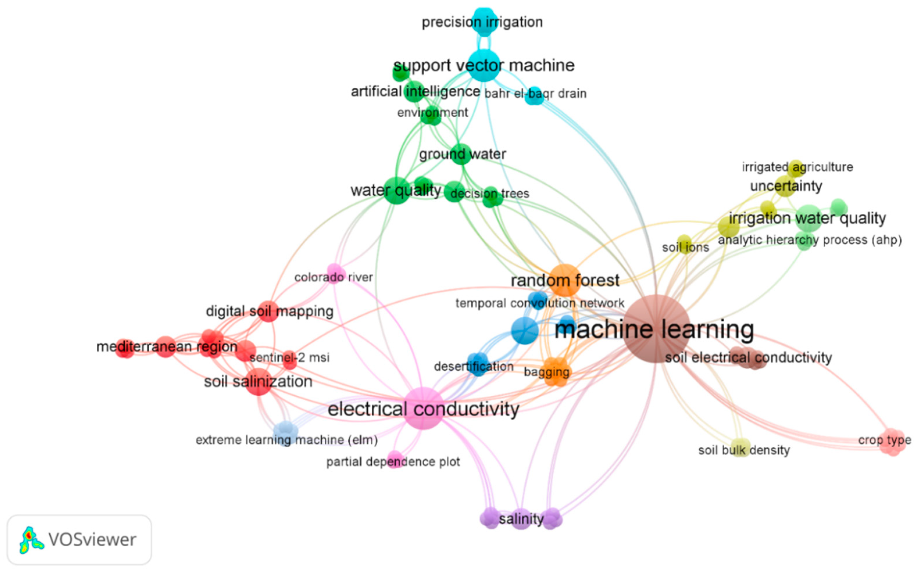
Synthesizing information from previous findings, this study extends the application of advanced AI integrated approaches to predict EC in the TWW. Based on the dominant feature selection framed with the key water quality parameters, this study put an effort to assure sustainable water use practices in agriculture, particularly in the Al-Qatif region, Saudi Arabia by utilizing the supervised ML techniques including SVR, ANFIS and MLR. The limited findings of the articles related to treated waste water, electrical conductivity, and machine learning in the Scopus database as shown in
Figure 1 suggested an underdeveloped area within the academic research domain, emphasizing the potential for additional exploration and in-depth investigation into predictive modeling techniques and system identification methods across the diverse disciplines related to water reuse.
2. Methodology
2.1. Study Area
In Al-Qatif, Saudi Arabia, the treated wastewater used for irrigation primarily originates from municipal wastewater treatment plants [
27]. The treatment plants receive wastewater from residential, commercial, and industrial sources within the city. Following comprehensive treatment processes designed to eliminate contaminants and pathogens, the treated water is then repurposed for irrigation in agricultural fields [
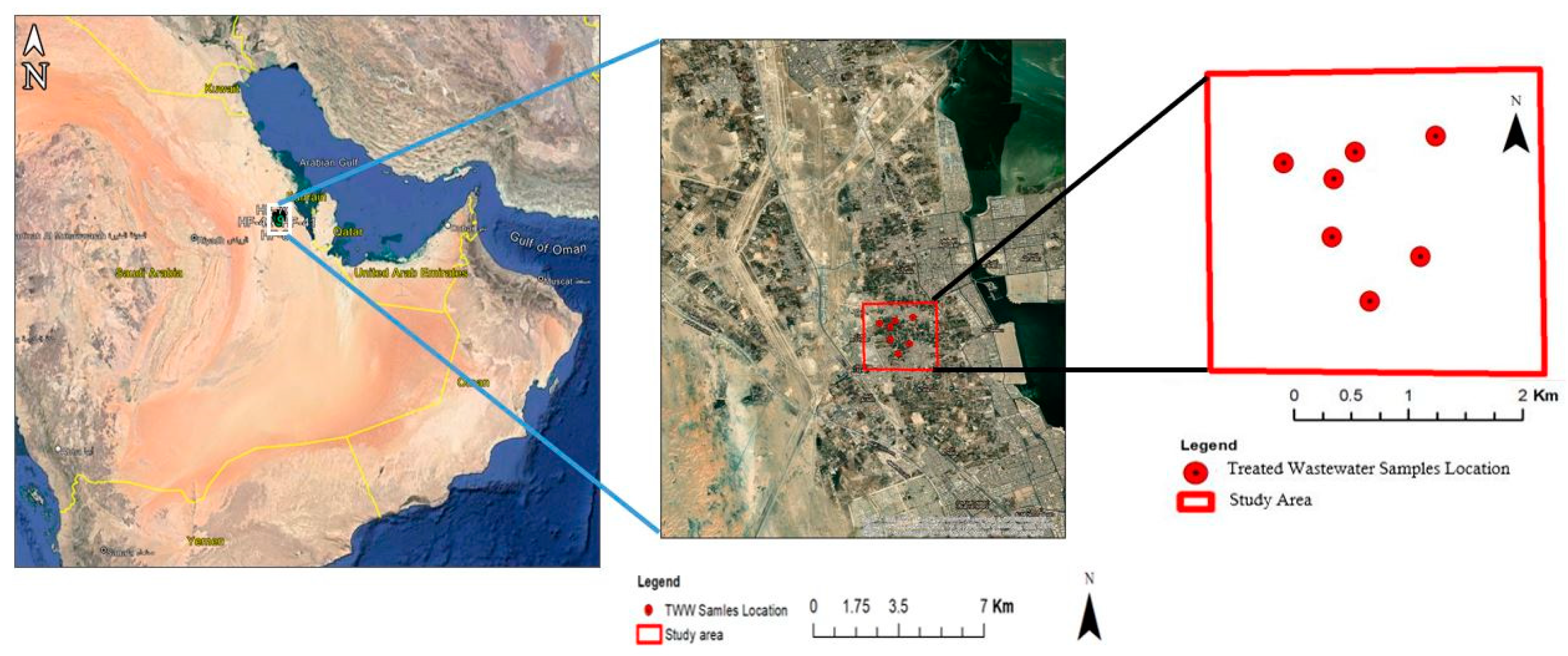
28]. This approach aids in the conservation of freshwater resources by repurposing treated wastewater that would otherwise be discharged into the environment. The treated wastewater undergoes various treatment steps, encompassing physical, biological, and advanced methods, to ensure it meets specific quality standards, rendering it safe for agricultural use. In this study, water samples were collected from various irrigation zones in Al-Qatif as shown in
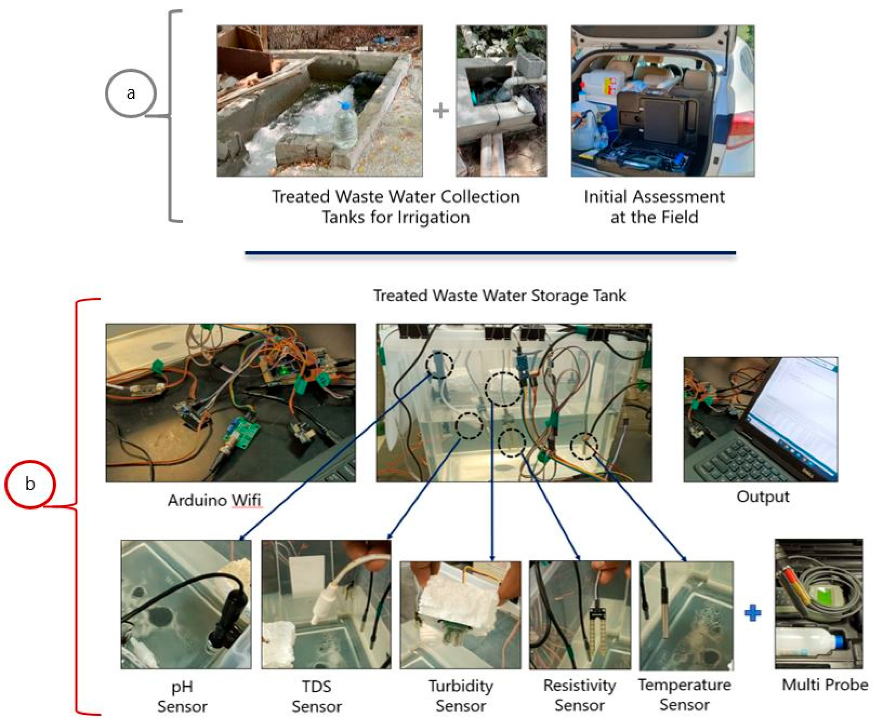
Figure 2. The TWW samples were assessed in the lab through a sensor-based real-time monitoring system integrated with Internet of Things (IoT) network and a multiprobe device as shown in
Figure 3. The key water quality parameters assessed involved, temperature (T), pH, Oxidation Reduction Potential (ORP), Resistivity (RES), Total Dissolved Solids (TDS), Salinity and Turbidity which served as the foundation for these models, given their profound influence on and their anticipated impact on EC levels.
2.2. Workflow Design
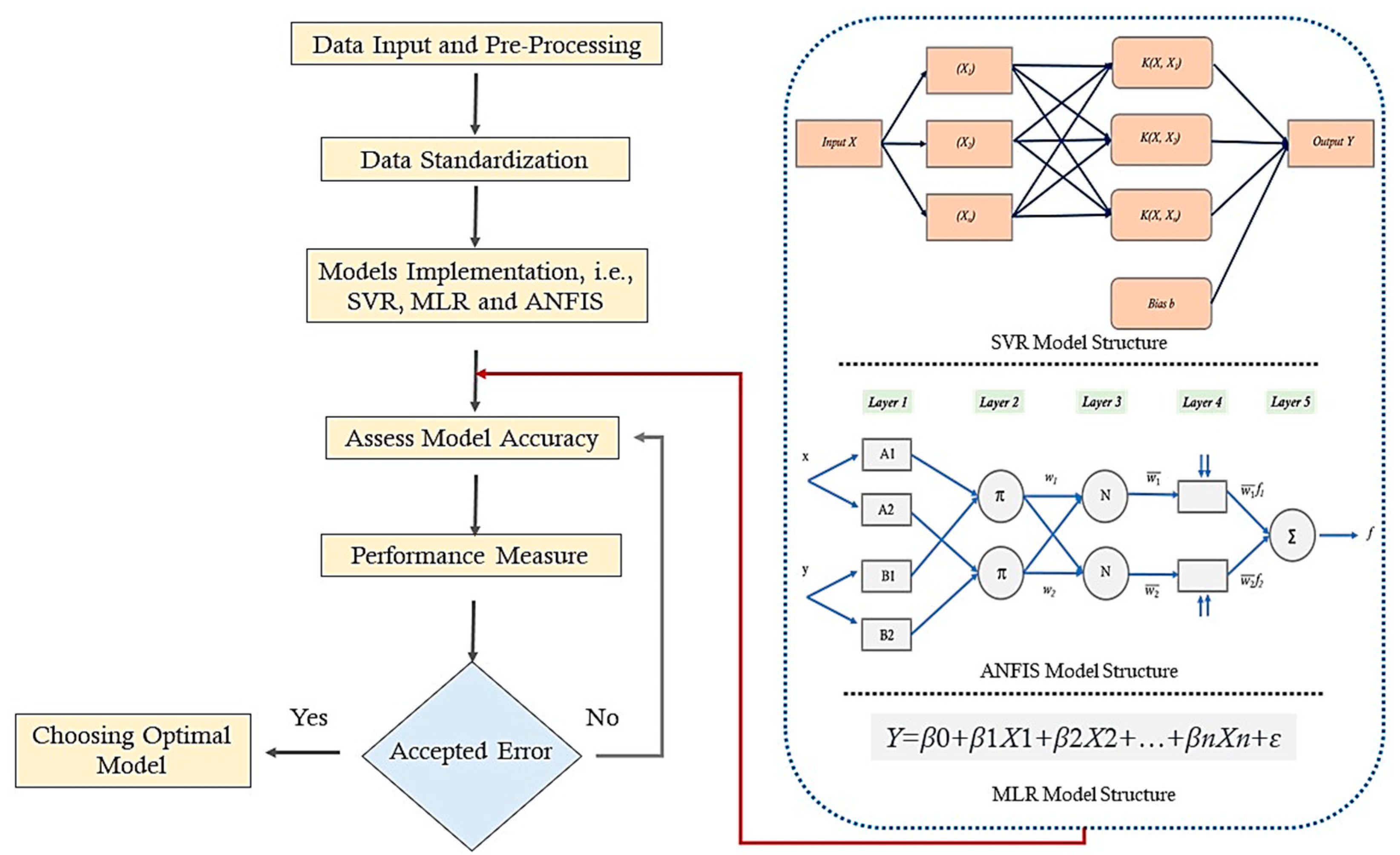
The implementation of SVR, ANFIS, and MLR models forms the foundational framework for achieving the research objectives. This paper outlines a systematic methodology commencing with data collection and preprocessing, ensuring dataset’s relevance for all three models. SVR was applied with a focus on data partitioning, model training, and hyperparameter optimization to establish an efficient classification framework, while ANFIS implementation involved steps such as fuzzy logic-based modeling, rule generation, and model training. Simultaneously, the MLR incorporated linear regression techniques tailored for optimal performance on the given dataset. The detailed approach depicted in the form of AI-Infused workflow can be illustrated in
Figure 4, providing a visual representation of the sequential steps and integration points between SVR, ANFIS, and MLR, while emphasizing the comprehensive nature of the proposed methodology.
2.3. Support Vector Regression (SVR)
SVR in artificial intelligence are employed for classification purposes [
28]. Their core function involves identifying an optimal hyperplane within a high-dimensional space to effectively separate different classes within a dataset. It has been widely used for a variety of applications for time-series, forecasting and parameter estimations [
29]. This is expressed by the fundamental equation:
The weight vector, denoted by w, the input vector, represented by x, and the bias component, denoted by b, constitute the hyperplane in the formula as stated in Eq. 1 with the aim to optimize the difference between the hyperplane and the closest reference points. SVR aims to create a strong decision boundary by minimizing inaccurate classifications and simultaneously optimizing the distance of separation between the groups [
30]. Moreover, it also exhibits expertise in labeled data settings by identifying a boundary that best classifies newly discovered, unseen data. Furthermore, the employment of kernel functions makes it easier for it to deal with non-linear data. By transforming the input space, these algorithms allow for linear separation in a feature space with greater dimensions. Thus, the adaptability and proficiency of SVR in handling intricate datasets make it a potent tool in artificial intelligence for a diverse range of classification tasks [
31].
2.4. Adaptive Network-based Fuzzy Inference System (ANFIS)
Adaptive neural networks and fuzzy logic concepts are usually combined with ANFIS to produce a flexible system for modeling complicated interactions [
32,
33] since it combines neural network learning power with fuzzy networks’ capacity to manage language ambiguity [
34]. It further helps to maximize the accuracy of the model by using a hybrid framework that combines neural network learning and rule-based fuzzy reasoning. Therefore, through a learning process, the model adjusts its parameters accordingly in order to concisely record and depict sophisticated patterns and connections in the data [
35,
36]. Moreover, the inference process of ANFIS may be used to describe its basic equation, where the output is given by a weighted sum of the firing strengths and consequent parameters of the prior membership functions. Mathematically, it can be represented as:
where,
represents the consequent parameter associated with each rule, and
denotes the firing strength of the corresponding antecedent membership function for each rule. This equation captures the essence of how ANFIS combines fuzzy logic and neural network principles for adaptive and effective modeling.
2.5. Multiple Linear Regression (MLR)
MLR is a statistical technique used in predictive modeling to analyze the relationship between a dependent variable and multiple independent variables [
37]. Unlike simple linear regression, which involves a single predictor, multiple linear regression considers two or more predictors [
38]. The model assumes a linear relationship between the dependent variable and each independent variable, allowing for the exploration of how these variables collectively contribute to predicting the outcome [
39]. The main equation for multiple linear regression is expressed as:
where, Y is the dependent variable,
,
, …
are the independent variables,
is the intercept,
,
, …
are the regression coefficients representing the impact of each independent variable, and ∈ is the error term accounting for unobserved factors affecting the dependent variable. The goal of multiple linear regression is to estimate the coefficients. (β values) that best fit the observed data and can be used to make predictions for new data.
2.6. Data and Evaluation Criteria
To forecast the EC and to assure the dependability of the chosen models, i.e., SVR, ANFIS and MLR, an extensive pre and post processing approach was used. At first, the data underwent a normalization process which aimed at bringing the variables to the standard range followed by a descriptive analysis which was done to get insights into the nature of the data and seek guidance in the process of feature selection. Next, the Pearson correlation matrix was employed to link the correlations between the obtained water quality metrices. It then led to the formation of a robust network which further helped in deciding the model combinations. Herein, the computed and the measured data was monitored through the four statistical measures, namely R2, R, MSE, and RMSE as discussed below:
where,
,
and
represents the predicted, observed and the observed electrical conductivity with its corresponding averages for N data points, respectively.
3. Results and Discussion
3.1. Performance Measure
Overall, the water parameters indicated a well-controlled and consistent composition within the specified range. In summarizing the key statistics, identifying the patterns and exploring the distribution of the values, the descriptive statistical analysis was performed which can be referred in
Table 1. Similarly, to assess the representation of how closely the pair of input variables are related to each other, the correlation matrix was used which can be referred in
Table 2. The findings highlighted in the table provided insights into the interdependencies among the studied parameters, emphasizing the complex dynamics of water quality in the given context [
40,
41].
Table 2 reveals significant correlations between the water quality measures that indicates a substantial connection among them. For example, Model I, which incorporates TDS and RES, demonstrated a higher correlation, suggesting a strong link with the EC. However, in recognition of their strong relationship, Model II further included the Temp and Sal. since the association between salinity and EC emphasizes their dependency, similarly, the temperature stresses its influence on EC. Thus, Model II combined TDS, RES, Temp, and Sal. to give a more comprehensive representation within the dataset. These chosen models provided an adequate and competent means of comprehending the relationships between the investigated water quality metrics by capturing the fundamental dynamics of those parameters. The selected two candidate models can be found as follow:
3.2. Predictive Analysis
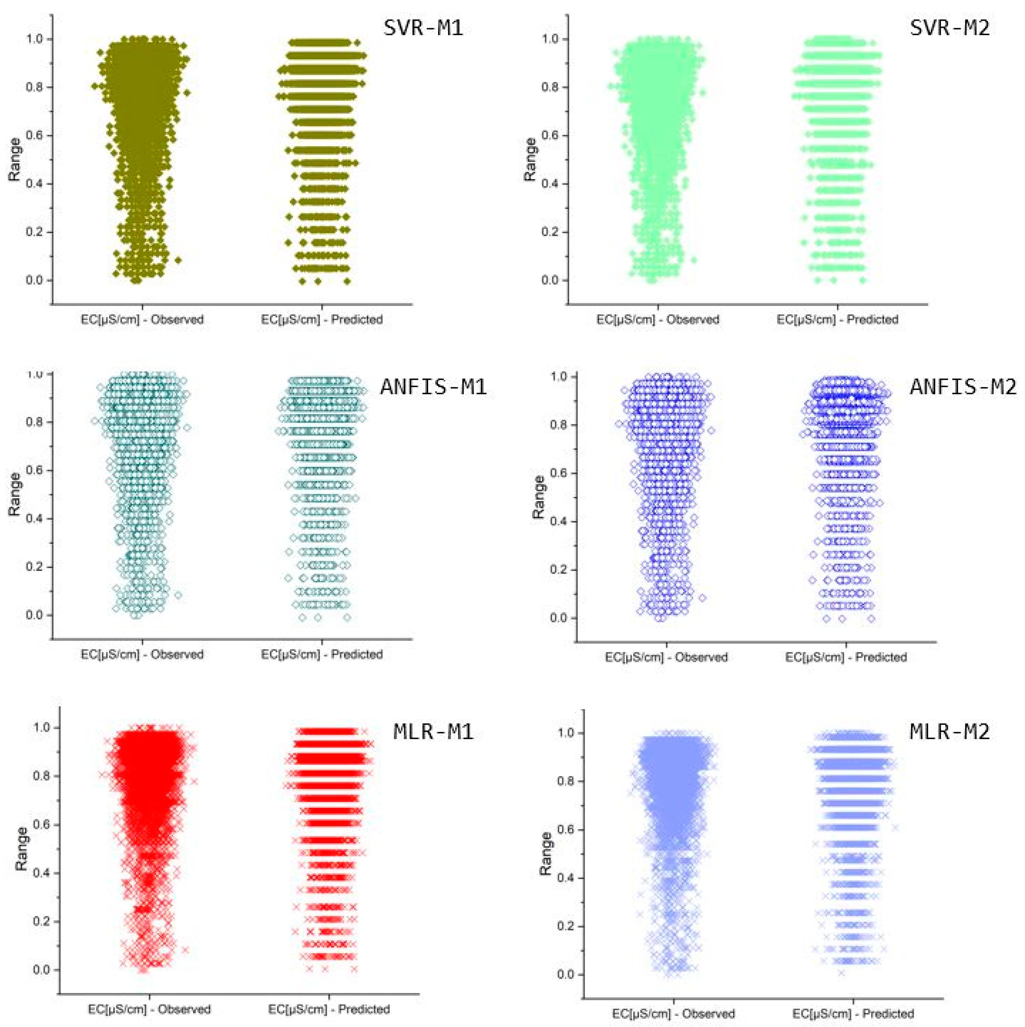
The use of various combination of variables across the unique models, namely Model I and Model II while employing SVR, ANFIS, and MLR was purposeful and carefully chosen to investigate diverse levels of complexity and information integration. This careful use of AI models emphasized the dedication to accuracy and flexibility in EC prediction, thus going beyond the traditional approaches. The response plots obtained through SVR, ANFIS, and MLR demonstrated a reliable and a close prediction based on the chosen water quality criteria in various modeling situations as seen in
Figure 5. It can therefore be stated that each method has its unique strengths, allowing to choose the most suitable approach based on the complexity and nature of the prediction task.
3.3. Calibration and Verification Phase
To further assure the resilience across the various datasets, extensive training and testing was done since these are the crucial steps in the development and evaluation which ensures that the model can generalize well to new, unseen data and perform effectively in real-world scenarios [
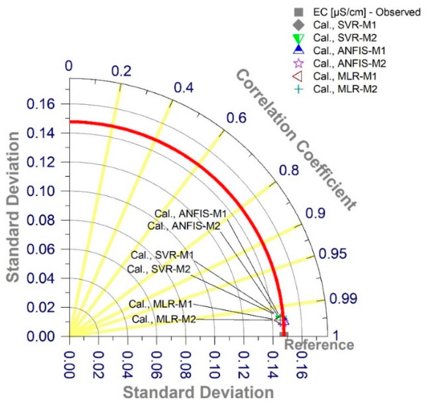
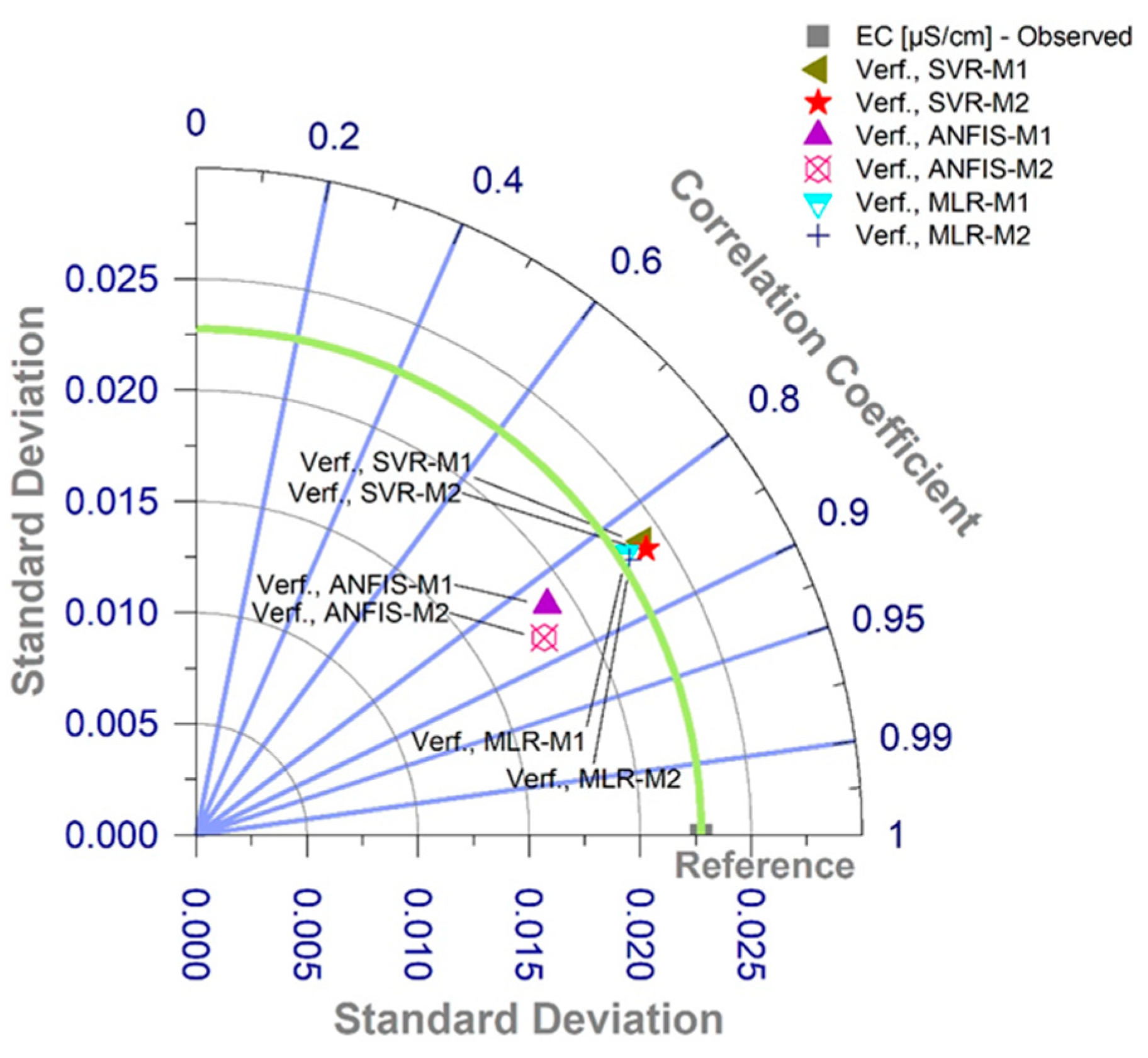
42]. The comparison among SVR, ANFIS and MLR each with its distinct configurations provided insights into their predictive abilities. Among these, ANFIS-M2 emerged as the standout performer with a commendable performance metric, indicating its superiority over the other models. The success of ANFIS-M2 is attributed to several factors that collectively contribute to its superior predictive accuracy for EC in treated wastewater. It is believed that the multiple relevant variables in the model allowed more comprehensive understanding of the complex interactions influencing the response variable. The higher R
2 value for ANFIS-M2 indicate its robustness and effectiveness in leveraging the combined information for improved EC prediction in treated wastewater as depicted by Taylor’s diagram as shown in
Figure 6 and
Figure 7 for both calibration and verification stages, respectively.
In the training phase, the performance metrics for the AI models, namely SVR-M1, SVR-M2, ANFIS-M1, ANFIS-M2, MLR-M1, and MLR-M2 were assessed as shown in
Table 3. The R
2 values, indicating the proportion of variance in the target variable explained by the models, were consistently high across all models, ranging from 0.9932 to 0.99572. Based on the provided R
2 values, it appears that the input variable selection in Eq. (9) performed exceptionally well across all the models indicating a better fit to the data. The model prediction capabilities of ANFIS-M2 (R
2: 0.99572) outperformed SVR-M1 (R
2: 0.99320), SVR-M2 (R
2: 0.99327), ANFIS-M1 (R
2: 0.99503), MLR-M1 (R
2: 0.99393), and MLR-M2 (R
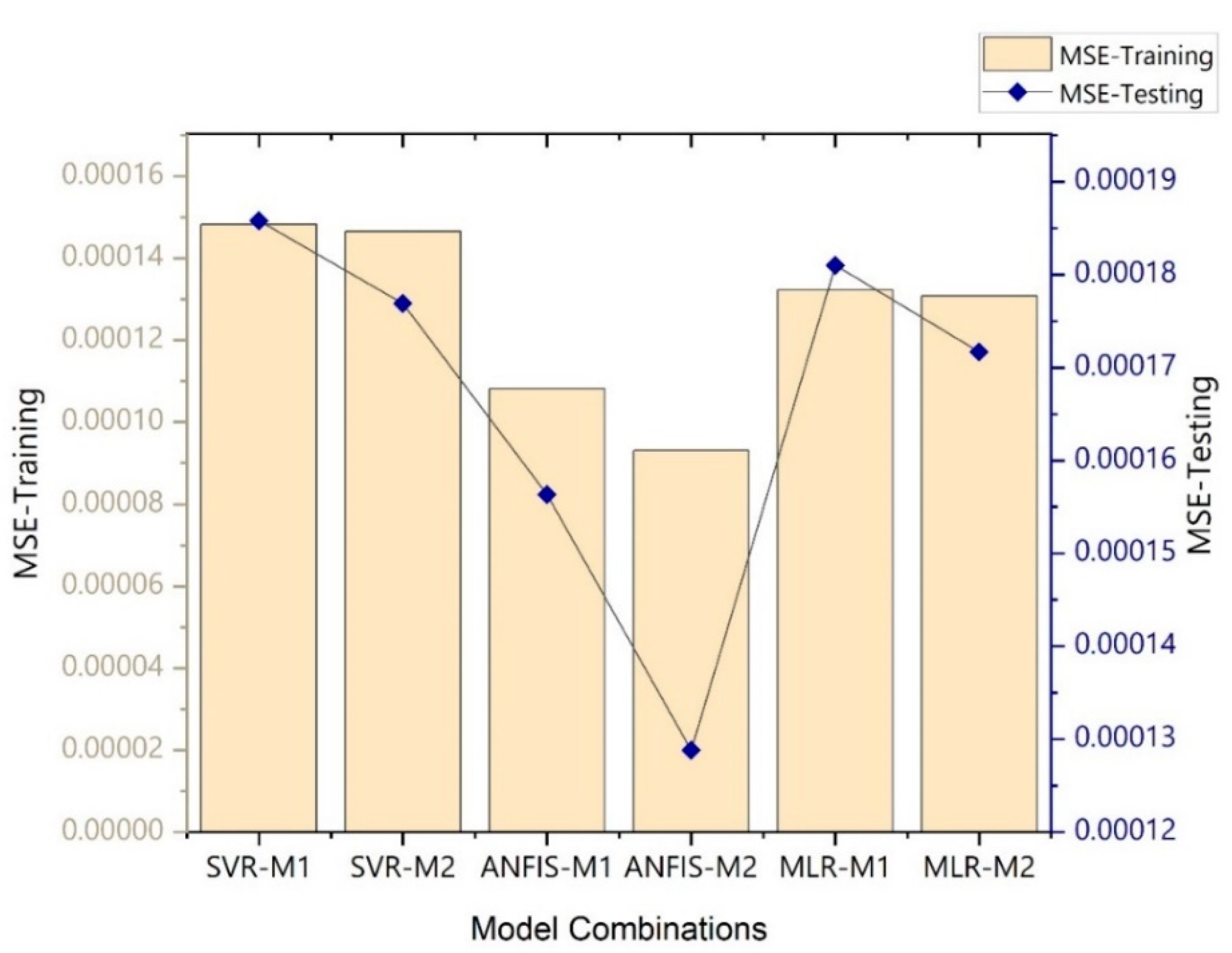
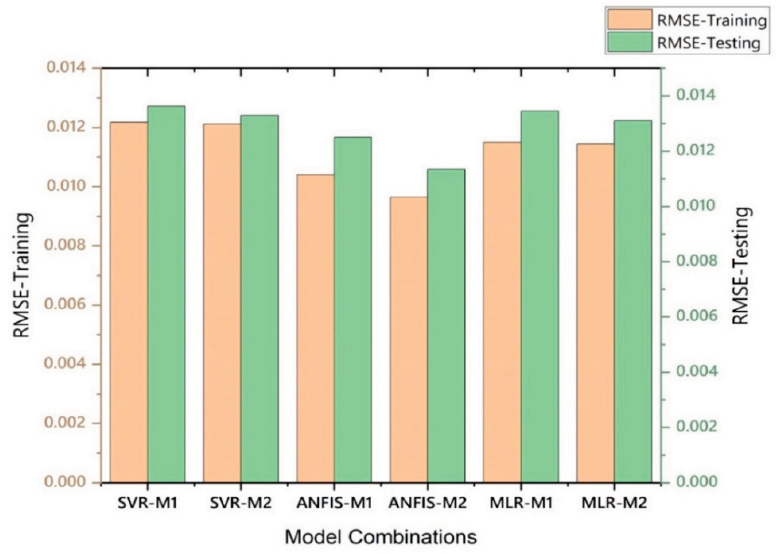
2: 0.99399). The correlation coefficient (R) values were also consistently close to 1, reflecting strong positive linear relationships between the predicted and actual values. The MSE and RMSE, measuring the accuracy and magnitude of prediction errors, showcased low values for all models, further highlighting their predictive capabilities. Since ANFIS-M2 exhibited the highest R
2 and the lowest MSE and RMSE among all models, this it suggests its superior performance in capturing the variance and minimizing prediction errors during the training phase.
During the testing phase, the performance of the models was assessed based on key metrics as shown in
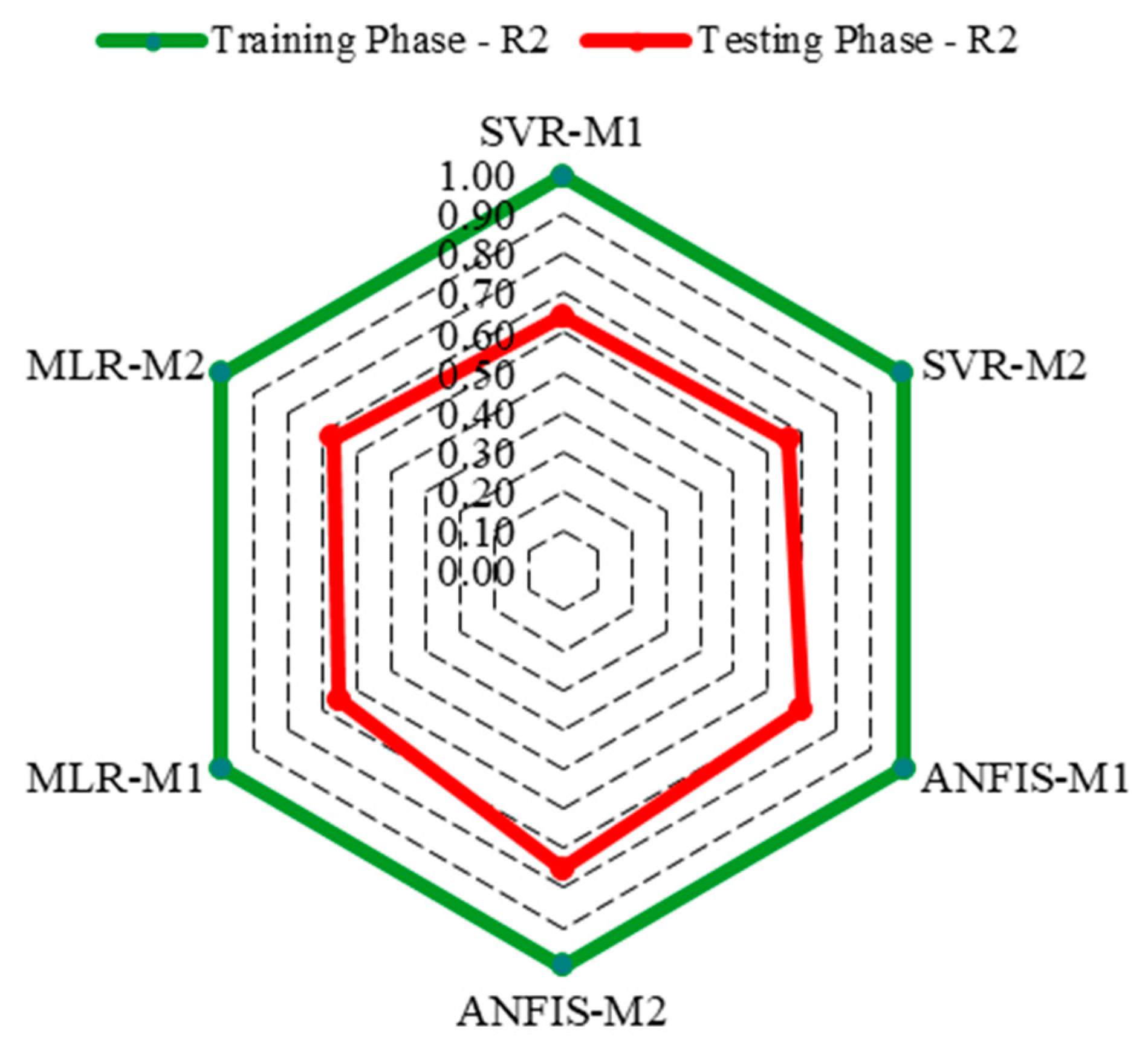
Table 4. Concerning R
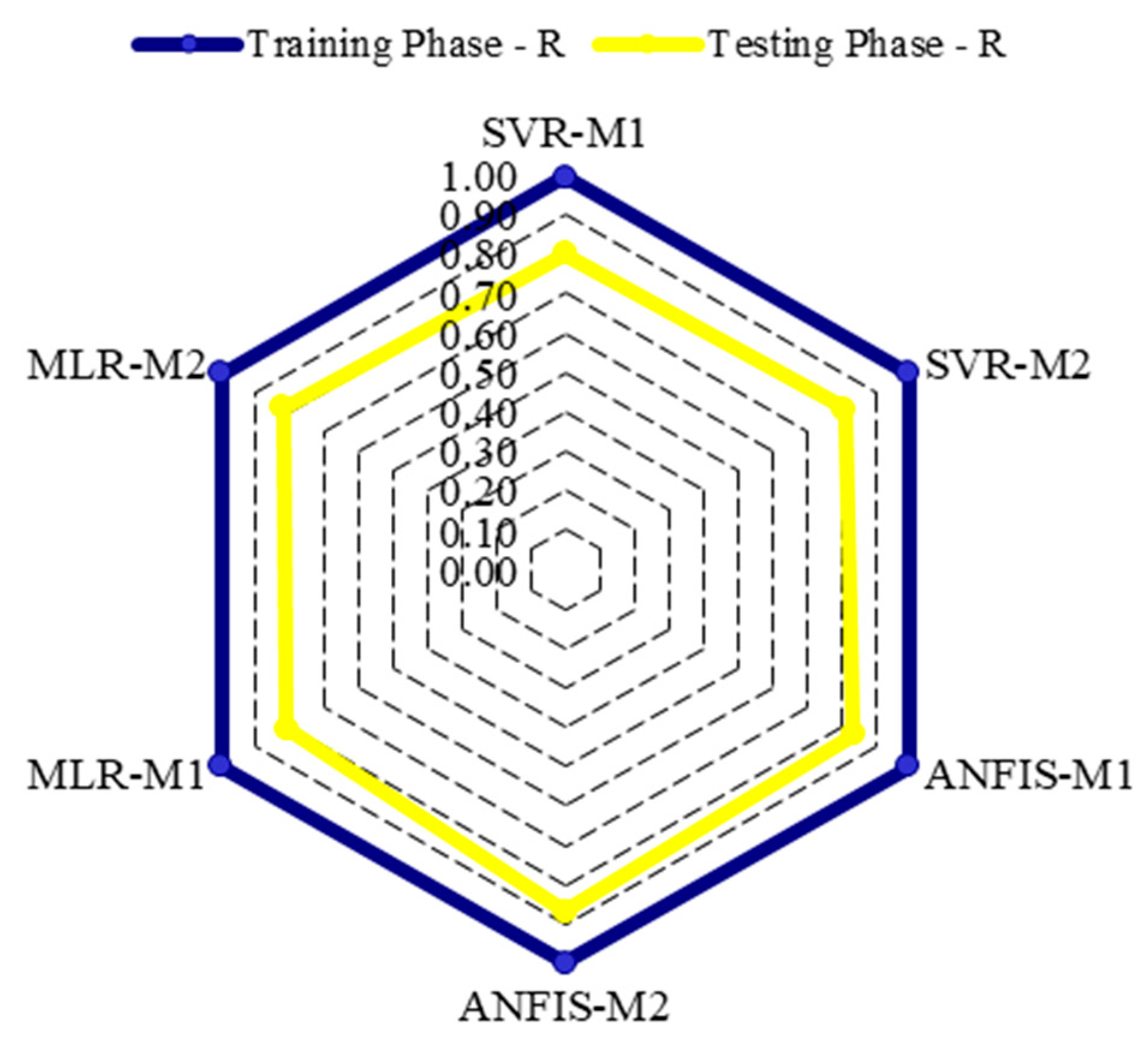
2, the values were in the range of 0.64142 for SVR-M1 to 0.75145 for ANFIS-M2. The predictive capability of ANFIS-M2 in the testing phase suggests that the corresponding model explains approximately 75.15% of the variability in the dependent variable, indicating a relatively strong fit. Similarly, for R, the values were in the range of 0.80088 for SVR-M1 to 0.86686 for ANFIS-M2, with ANFIS-M2 again showing the strongest correlation. In terms of MSE and RMSE, both indicating the magnitude of prediction errors, ANFIS-M2 achieved the lowest values (MSE: 0.00012, RMSE: 0.01134), emphasizing its superior predictive accuracy. Thus, it can be said that in the testing phase, ANFIS-M2 outperformed the other models which confirms its effectiveness in capturing the underlying patterns within the given data set and making accurate predictions.
The radar graphs as depicted in
Figure 8 and
Figure 9 highlight a thorough comparison of each model’s performance, i.e., R
2 and R, and provide an important insight regarding its efficacy at various training and testing stages on a circular grid. The radial nature of the graph allowed to gain a detailed picture of each models’ performance at various points during calibration and verification stages. Similarly, the comprehensive bar graphs as shown in
Figure 10 and
Figure 11, illuminates the differences in performance and errors displayed by each model. By presenting a visual breakdown of the models’ performance metrics, these bar graphs served as a valuable supplement to the radar graphs, enabling a more in-depth interpretation of the efficacy of each model.
4. Conclusions
The in-depth investigation of water quality indicators combined with real-time monitoring under supervised machine learning has significantly improved our comprehension of salinity dynamics. In the training phase, all models performed exceptionally well based on the evaluation criteria suggesting a great capacity to capture variation within the given data set. The low MSE an RMSE values further affirmed the models’ capabilities in minimizing the prediction errors. However, it was noticed that during the testing phase, the outcomes exhibited a decrease in strength. This indicates that while the models performed exceptionally well on the training data, it encountered challenges in generalizing to unseen data. Thus, there seems a need for further careful consideration and potential refinement of the models to enhance their robustness and generalization capabilities. For future work, it is advised to investigate methods for enhancing model generalization in subsequent work, such as adjusting hyperparameters, adding more features, or using more complex model architectures. Furthermore, evaluating how data variability and possible outliers affect model performance may help improve the models’ suitability for use in real-world scenarios. However, the environmental significance of integrating hybrid techniques coupled with treated wastewater assessment to optimize agricultural water reuse in the Al-Qatif region of Saudi Arabia is multifaceted, addressing several critical issues related to water resources management, agricultural sustainability, and environmental conservation. For example, (i) water scarcity mitigation: Saudi Arabia is one of the most water-scarce countries in the world, relying heavily on non-renewable groundwater and desalination for its water supply. Integrating hybrid techniques for wastewater treatment and reuse can significantly contribute to mitigating water scarcity by providing an alternative source of water for agriculture, which is a major consumer of freshwater resources. This aligns with global efforts and studies emphasizing the importance of treated wastewater as a resource for addressing water scarcity (ii) sustainable agriculture: By using treated wastewater for irrigation, agricultural practices in Al-Qatif can become more sustainable. This not only reduces the reliance on scarce freshwater resources but also can improve soil health through the addition of nutrients present in treated wastewater. Studies have shown that appropriate use of treated wastewater can enhance crop yields and reduce the need for chemical fertilizers (iii) environmental protection: Proper treatment and reuse of wastewater help in protecting water bodies from pollution. By treating wastewater to appropriate standards before use in agriculture, the risk of contaminating soil and groundwater with pathogens, heavy metals, and other pollutants is significantly reduced. This is crucial for maintaining ecosystem health and biodiversity (iv) economic benefits: The integration of hybrid wastewater treatment technologies can lead to economic benefits by reducing the costs associated with freshwater extraction and treatment, as well as by potentially increasing agricultural productivity. This can contribute to the economic viability of agricultural practices in arid and semi-arid regions and (v) climate change adaptation: Utilizing treated wastewater in agriculture is also seen as a strategy for climate change adaptation, helping communities to cope with the increased variability in water supply and demand. It provides a buffer against drought conditions, which are expected to become more frequent and severe with climate change.
Author Contributions
Conceptualization, S.M.H.S., S.I.A., and M.A.Y.; Data curation, S.M.H.S., S.I.A., F.A., and M.A.Y.; Funding acquisition, S.S.S., D.U.L., and C.B.P.; Investigation, S.I.A.; Methodology, S.I.A., S.M.H.S., M.A.Y., Z.M. and E.H.H.A.; Project administration, I.H.A.; Resources, I.H.A.; Supervision, I.H.A.; Writing—original draft, S.I.A., S.M.H.S., and M.A.Y., Writing—review and editing, S.I.A., Z.M., S.S.S., and C.B.P.
Funding
This research was funded by the Deanship of Research Oversight and Coordination (DROC) at King Fahd University of Petroleum & Minerals (KFUPM) under the Interdisciplinary Research Center for Membranes and Water Security.
Data Availability Statement
The data presented in this study are available on request from the corresponding author.
Acknowledgments
The authors would like to acknowledge all support from the Interdisciplinary Research Center for Membranes and Water Security, King Fahd University of Petroleum and Minerals.
Conflicts of Interest
The authors declare no conflict of interest.
References
- Li, Y.; Mi, W.; Ji, L.; He, Q.; Yang, P.; Xie, S.; Bi, Y. Urbanization and Agriculture Intensification Jointly Enlarge the Spatial Inequality of River Water Quality. Sci. Total Environ. 2023, 878, 162559. [Google Scholar] [CrossRef]
- Kouadri, S.; Elbeltagi, A.; Islam, A.; Kateb, S. Performance of Machine Learning Methods in Predicting Water Quality Index based on Irregular Data Set: Application on Illizi Region (Algerian Southeast). Appl. Water Sci. 2021, 11, 1–20. [Google Scholar] [CrossRef]
- Liang, W.; Zhang, W.; Jin, Z.; Yan, J.; Li, Y.; Yu, Q. Rapid Urbanization and Agricultural Intensification Increase Regional Evaporative Water Consumption of the Loess Plateau. J. Geophys. Res. Atmos. 2020, 125, 1–26. [Google Scholar] [CrossRef]
- Bilali, A.; Taleb, A. Prediction of Irrigation Water Quality Parameters Using Machine Learning Models in a Semi-Arid Environment. J. Saudi Soc. Agric. Sci. 2020, 19, 439–451. [Google Scholar] [CrossRef]
- Busico, G.; Kazakis, N.; Cuoco, E.; Colombani, N.; Tedesco, D.; Voudouris, K.; Mastrocicco, M. A Novel Hybrid Method of Specific Vulnerability to Anthropogenic Pollution Using Multivariate Statistical and Regression Analyses. Water Res. 2020, 171, 115386. [Google Scholar] [CrossRef] [PubMed]
- She, Y.; Chen, J.; Zhou, Q.; Wang, L.; Duan, K.; Wang, R.; Qu, S.; Xu, M.; Zhao, Y. Evaluating Losses from Water Scarcity and Benefits of Water Conservation Measures to Intercity Supply Chains in China. Environ. Sci. Technol. 2024, 58, 1119–1130. [Google Scholar] [CrossRef] [PubMed]
- Mishra, S.; Kumar, R.; Kumar, M. Use of Treated Sewage or Wastewater as an Irrigation Water for Agricultural Purposes- Environmental, Health, and Economic Impacts. Total Environ. Res. Themes. 2023, 6, 100051. [Google Scholar] [CrossRef]
- Neelofar, M.; Bhat, S.; Muslim, M. Water Auditing and Recycling as a Tool for Management of Water Resources: An Indian Perspective. Appl. Water Sci. 2023, 13, 1–14. [Google Scholar] [CrossRef]
- Shahid, S.; Ahmed, M. Environmental Cost and Face of Agriculture in the Gulf Cooperation Council Countries. Environ. Cost Face Agric. Gulf Coop. Counc. Ctries, 2014; pp. XXXIV, 186, ISBN 978-3-319-05767-5. [Google Scholar]
- Younos, T.; Parece, T. Sustainable Water Management in Urban Environments. The Handbook of Environ. Che. 47, 2016; pp. XVIII, 332, ISBN 978-3-319-29337-0. [Google Scholar]
- World Health Organization (WHO). Reuse of Effluents-Methods of Wastewater Treatment and Health Safeguards. World Health Organ Tech Rep Ser 1973, 517, 1–63. [Google Scholar]
- World Health Organization (WHO). Health Guidelines for the use of Wastewater in Agriculture and Aquaculture. Report of a WHO Scientific Group. World Health Organ Tech Rep Ser. 1989, 778, 1–74. [Google Scholar]
- World Health Organization (WHO). WHO Guidelines for the Safe use of Wastewater Excreta and Greywater. 2006.
- Ayers, R.; Wescott, D. Water Quality for Agriculture; Food and Agriculture Organization (FAO): Rome, Italy, 1985; p. 174. [Google Scholar]
- Food and Agriculture Organization (FAO). Wastewater Treatment and Use in Agriculture. Available online: http://www.fao.org/docrep/T0551E/T0551E00.htm. (accessed on 01 March 2024).
- Environmental Protection Agency (EPA). Guidelines for Water Reuse; U.S. Environmental Protection Agency: Washington, DC, USA, 2004. [Google Scholar]
- Environmental Protection Agency (EPA); U.S. Agency for International Development. Guidelines for Water Reuse; U.S. Environmental Protection Agency: Washington, DC, USA, 2012. [Google Scholar]
- Chen, Z.; Ngo, H.; Guo, W. A Critical Review on the End Uses of Recycled Water. Critical Rev. in Environ. Sci. and Tech. 2013, 43, 1446–1516. [Google Scholar] [CrossRef]
- Al Hadidi, N.; Al Hadidi, M. Suitability of Reclaimed Wastewater Effluent from Decentralized Wastewater Plant for Irrigation. Appl. Water Sci. 2021, 11, 1–11. [Google Scholar] [CrossRef]
- Pásztor, L.; Takács, K.; Mészáros, J.; Szatmári, G.; Árvai, M.; Tóth, T.; Barna, G.; Koós, S.; Kovács, Z.; László, P.; Balog, K. Indirect Prediction of Salt Affected Soil Indicator Properties through Habitat Types of a Natural Saline Grassland Using Unmanned Aerial Vehicle Imagery. Land, 2023, 12, 1516. [Google Scholar] [CrossRef]
- Kouassi, D.; Kouame, I.; Koffi, K.; Douagui, A.; Sandu, A.; Sandu, I. Assessment of the Quality of Quaternary Groundwater Under the Influence of Anthropogenic Activities in the Low-Income Neighbourhoods of the Treichville Municipality (Abidjan, Côte d’Ivoire). SN Appl. Sci. 2020, 2, 1–19. [Google Scholar] [CrossRef]
- Singh, A. Soil Salinization Management for Sustainable Development: A Review. J. Environ. Manage. 2021, 277, 111383. [Google Scholar] [CrossRef] [PubMed]
- Khamidov, M.; Ishchanov, J.; Hamidov, A.; Donmez, C.; Djumaboev, K. Assessment of Soil Salinity Changes under the Climate Change in the Khorezm Region, Uzbekistan. Int. J. Environ. Res. Public Health. 2022, 19, 8794. [Google Scholar] [CrossRef]
- Taghizadeh-Mehrjardi, R.; Schmidt, K.; Toomanian, N.; Heung, B.; Behrens, T.; Mosavi, A.; Band, S.; Amirian-Chakan, A.; Fathabadi, A.; Scholten, T. Improving the Spatial Prediction of Soil Salinity in Arid Regions Using Wavelet Transformation and Support Vector Regression Models. Geoderma. 2021, 383, 114793. [Google Scholar] [CrossRef]
- Najah, A.; El-Shafie, A.; Karim, O.; El-Shafie, A. Performance of ANFIS Versus MLP-NN Dissolved Oxygen Prediction Models in Water Quality Monitoring. Environ. Sci. Pollut. Res. 2014, 21, 1658–1670. [Google Scholar] [CrossRef] [PubMed]
- Khadr, M.; Elshemy, M. Data-Driven Modeling for Water Quality Prediction Case Study: The Drains System Associated with Manzala Lake, Egypt. Ain Shams Eng. J. 2017, 8, 549–557. [Google Scholar] [CrossRef]
- Saleem, M. Microbial Evaluation of Al-Khobar Wastewater Treatment Plant. MSc. Thesis in Civil Engineering—King Fahd University of Petroleum & Minerals 1997. [Google Scholar]
- Alsharhan, A.; Rizk, Z.; Nairn, A.; Bakhit, D.; Alhajari, S. Hydrogeology of an Arid Region: The Arabian Gulf and Adjoining Areas. In Elsevier Sci; 2001; ISBN 978-0-444-50225-4. [Google Scholar]
- Niazmardi, S.; Khanahmadlou, H.; Shang, J.; McNairn, H.; Homayouni, S. A New Classification Method Based on the Support Vector Regression of NDVI Time Series for Agricultural Crop Mapping. 2nd Int. Conf. Agro-Geoinformatics Inf. Sustain. Agric. Agro-Geoinformatics 2013, 361–364. [Google Scholar]
- Jayanthi, S.; Keesara, V.; Sridhar, V. Prediction of Future Lake Water Availability Using SWAT and Support Vector Regression (SVR). Sustain. 2022, 14, 6974. [Google Scholar] [CrossRef]
- Mustafa, H.; Hayder, G.; Abba, S.; Algarni, A.; Mnzool, M.; Nour, A. Performance Evaluation of Hydroponic Wastewater Treatment Plant Integrated with Ensemble Learning Techniques: A Feature Selection Approach. Processes. 2023, 11, 478. [Google Scholar] [CrossRef]
- Sayari, S.; Mahdavi-Meymand, A.; Zounemat-Kermani, M. Irrigation Water Infiltration Modeling Using Machine Learning. Comput. Electron. Agric. 2021, 180, 105921. [Google Scholar] [CrossRef]
- Azad, A.; Karami, H.; Farzin, S.; Saeedian, A.; Kashi, H.; Sayyahi, F. Prediction of Water Quality Parameters Using ANFIS Optimized by Intelligence Algorithms (Case Study: Gorganrood River). KSCE J. Civ. Eng. 2018, 22, 2206–2213. [Google Scholar] [CrossRef]
- Kisi, O.; Murat, A. Comparison of ANN and ANFIS Techniques in Modeling Dissolved Oxygen. Sixt. Int. Water Technol. Conf. 2012, 1–10. [Google Scholar]
- Jalalkamali, A. Using of Hybrid Fuzzy Models to Predict Spatiotemporal Groundwater Quality Parameters. Earth Sci. Informatics. 2015, 8, 885–894. [Google Scholar] [CrossRef]
- Chiu, S. Fuzzy Model Identification based on Cluster Estimation. J. Intell. Fuzzy Syst. 1994, 2, 267–278. [Google Scholar] [CrossRef]
- Keskin, T.; Özler, E.; Şander, E.; Düğenci, M.; Ahmed, M. Prediction of Electrical Conductivity Using ANN and MLR: A Case Study from Turkey. Acta Geophys. 2020, 68, 811–820. [Google Scholar] [CrossRef]
- Mattas, C.; Dimitraki, L.; Georgiou, P.; Venetsanou, P. Use of Factor Analysis (Fa), Artificial Neural Networks (ANNs) And Multiple Linear Regression (MLR) For Electrical Conductivity Prediction in Aquifers in the Gallikos River Basin, Northern Greece. Hydrology, 2021, 8, 127. [Google Scholar] [CrossRef]
- Chenini, I.; Khemiri, S. Evaluation of Ground Water Quality Using Multiple Linear Regression and Structural Equation Modeling, Int. J. Environ. Sci. Technol. 2009, 6, 509–519. [Google Scholar]
- Abba, S.; Nourani, V.; Elkiran, G. Multi-Parametric Modeling of Water Treatment Plant Using AI-Based Non-Linear Ensemble. J. Water Supply Res. Technol. 2019, 68, 547–561. [Google Scholar] [CrossRef]
- Nourani, V.; Elkiran, G.; Abba, S. Wastewater Treatment Plant Performance Analysis Using Artificial Intelligence—An Ensemble Approach. Water Sci. Technol. 2018, 78, 2064–2076. [Google Scholar] [CrossRef]
- Aldoseri, A.; Al-Khalifa, K.; Hamouda, A. Re-Thinking Data Strategy and Integration for Artificial Intelligence: Concepts, Opportunities, and Challenges. Appl. Sci. 2023, 13, 7082. [Google Scholar] [CrossRef]
|
Disclaimer/Publisher’s Note: The statements, opinions and data contained in all publications are solely those of the individual author(s) and contributor(s) and not of MDPI and/or the editor(s). MDPI and/or the editor(s) disclaim responsibility for any injury to people or property resulting from any ideas, methods, instructions or products referred to in the content. |
© 2024 by the authors. Licensee MDPI, Basel, Switzerland. This article is an open access article distributed under the terms and conditions of the Creative Commons Attribution (CC BY) license (http://creativecommons.org/licenses/by/4.0/).
