1. Introduction
Bacillus anthracis is the bacteria that causes the infectious disease called anthrax. Both domestic and wild animals are affected by the disease. When vulnerable individuals come into touch with diseased animals or eat tainted dairy and animal products, they can get the anthrax virus. A zoonotic disease called anthrax is naturally occurring in soil and affects populations of humans and animals globally. People can get sick from tainted animal products or by having close contact with animals [
1,
2]. Infected animals, especially livestock, may die suddenly and unexpectedly from it, and it can occasionally be dangerous to people. Anthrax may generally be spread to animals in two ways: either by consuming a significant amount of spores found in soil or on plants, or by stable insects called Stomoxys calcitrans, which feed on contaminated blood that leaks from the remains of animals that have contracted the disease [
3,
4]. By applying immunizations before exposure, is the only effective way to control anthrax and is advisable to do so between 2-4 weeks prior to the anticipated endemic season [
3]. Anthrax spores may survive for up to two centuries because of their remarkable resilience to temperature fluctuations, desiccation, heat, and a range of chemical agents [
5]. Furthermore, in cattle, anthrax infections frequently worsen without showing any signs (symptoms) [
3]. The time frame in such a scenario could be critical for averting anthrax outbreaks.
In addition to herbivorous animals, predators that eat the contaminated carcasses of anthrax-infected prey are also at risk from anthrax. However, compared to herbivores, carnivores often have lower infection and death rates. According to the World Health Organization (WHO), the World Anthrax Data Site has recorded anthrax outbreaks in animals from around 200 nations, especially in areas with large populations of both humans and animals. For example, the exact reason of the anthrax deaths of a variety of animals in Etosha National Park, including ostriches and elephants, was still unclear. Three captive cheetahs were reported dead in November 2004 at the Jwana Game Reserve in Jwanen, Botswana, Meat from deceased red hartebeest infected with anthrax had been given to them [
6,
7]. Africa, the Middle East, and Asia have relatively high rates of anthrax infection in wild animals and livestock, with periodic outbreaks and epizootics [
8]. Anthrax is quite widespread in Bangladesh and India, two nations in southern Asia, outbreaks and diseases in both humans and animals are often reported [
9,
10]. If treatment measures are not taken, the most common cutaneous type of anthrax infection can have a morbidity(fatality) rate of up to 20%; however, with appropriate treatment, it can drop to less than 1% [
11].
Both natural phenomena and the dynamics of infectious disease transmission may be explained by mathematical models. In epidemiology, these models are essential for controlling infectious diseases. These models are able to clearly describe the dynamics and mechanisms of disease transmission [
12,
13]. Lotka and Volterra introduced the field of prey-predator ecosystem in mathematical research, which was termed lotka-voltera model [
14,
15]. In mathematical modeling, Kermack and Kendrick coined the term "epidemiology" and investigated an SEIRS compartment model [
16]. For a while now, there have been proposals and research done on complex models for the transmission dynamics of diseases, including periodic orbits, Hoff bifurcations, and multiple equilibria. They provide a clear qualitative depiction of the dynamics of the disease, together with improved analysis and consequences for disease forecasting [
17,
18]. The authors of [
1] examined how a continuous vaccine affected an anthrax model, but they never took into account the consequences of the best possible control. Based on their studies, theoretical findings under continuous vaccination, the disease model's transmission resembles dynamics in the absence of vaccination. Additionally, [
19] created a model by taking the influence of vaccines into account and came to the conclusion that the ideal vaccination coverage threshold needed for disease elimination. On the other hand, [
20] employed optimum control while examining a nonlinear SIR epidemic model that included a vaccination plan.
No nation can really declare itself free of anthrax since the disease's spores may survive for a very long period in the soil. Nonetheless, anthrax epidemics tend to occur more often in developing nations. Furniss and Hahn conducted groundbreaking research on anthrax modeling from a mathematical modeling standpoint when they examined an anthrax epizootic in South Africa's Kruger National Park [
21]. The same researchers put up a different deterministic model with some threshold findings in 1983 [
22]. Friedman and Yakubu added elements like as migration, growth, and the host's natural death [
23] to the model put forward by Hahn and Furniss [
20] adding a predetermined time delay. Mushayabasa suggested a fresh approach that was based on the model of Hahn and Furniss [
22]. The function of human labor (as a control mechanism) in cleaning up contaminated carcasses, including the soil or surrounding region, is also included in their model [
24]. Two distinct models investigating the spread and management of anthrax infection within two frameworks were provided by Mushayabasa et al. They investigated the effects of the incubation time and carcass clearance in the first framework. They looked at how the vector population affected the transmission and management of anthrax in the second approach [
25]. Using vaccination as a control, Kimathi and Wainaina [
26] looked at the dynamics of anthrax spread in animal populations. The co-dynamics of anthrax and listeriosis infections were investigated, and the qualitative and quantitative link between them within preventative and treatment strategies was researched by Osman et al. [
27]. According to their research, anthrax infection may raise the chance of Listeriosis, but listeriosis disease itself is not linked to an increased risk of anthrax. Their results show that while listeriosis infection is not linked to an increased risk of anthrax infection, anthrax infection is associated with a higher likelihood of listeriosis infection. Rezapour et al. suggested a novel fractional ordered model in the sense of the Caputo-Fabrizio fractional derivative [
28], which was inspired by the work of Kimathi et al. They examined the asymptotic stability of the equilibrium states that are endemic and disease-free in order to calculate the fundamental reproduction number R0, of the fractional system.
Researchers' interest in disease modeling, particularly the modeling of diseases like HIV and cancer, has increased recently. The SARS-CoV-2 virus is the source of the COVID-19 pandemic, which has lately garnered a lot of attention with over 21 million confirmed cases and 758,000 fatalities recorded. During the COVID-19 epidemic, mathematical models were essential in predicting different waves, and research in this field is still ongoing [
29].
Our examination of the literature indicates that, compared to diseases like cancer or HIV, modeling anthrax disease has received comparatively less attention from researchers. The ongoing threat that anthrax poses in developing nations (Africans and the likes) is a strong incentive for us to investigate the mathematical modeling of anthrax in this research work
Epidemiology of Anthrax in Nigeria
Following the discovery of widespread death resulting from pathognomonic signs of the disease in a multi-species farm in Gajiri Village, Suleja, Niger State, Nigeria's index anthrax case was confirmed. Nigerian Center for Disease Control (NCDC). About 100 cows (49 foreign and 51 native varieties), 73 sheep (a breed of fat-tailed sheep from Sudan), and 19 goats were present on the property where the index case was located. On June 27, 2023. The circumstances that led to the verified anthrax epidemic began. Thirteen cattle and ten sheep were among the thirty-five instances (twenty cattle and fifteen sheep) that had been reported as of July 13, 2023 the day the samples were collected. The national reference laboratory made a confirmation diagnosis of anthrax on July 16, 2023 ((Nigerian Veterinary Research Institute). VOM, Plateau State, although animals are driven to graze on natural grass, the majority of the cows were grown in large production systems. On July 19, 2023, the global disease notice was transmitted to the World Animal Health Information system, and an urgent notification was issued to the World Organization for Animal Health on July 17, 2023.
In addition, more research is being done to determine the infection's origin and how it spread to other farms and people. Although reports of human exposure exist, none of human symptoms or deaths have been documented yet. To identify, isolate, and monitor all affected individuals, the FMARD and the Nigeria Centre for Disease Control and Prevention (NCDC) are presently collaborating closely with the Ministries of Agriculture and Health of Niger State. The incident manager has been designated by the NCDC to ensure efficient response coordination, and the incident management system (IMS) has been activated at level two (2). The probability of an epidemic and its possible effects on humans were rated as HIGH in the risk assessment carried out by the human health sector. (NCDC).
Treatment of Anthrax
Adequate immunization of vulnerable vector populations lowers the likelihood of spreading to humans because the disease is a zoonotic and preventable by recommended vaccine. Therefore, minimizing contact with diseased vectors and managing vector with anthrax effectively removes the danger to humans. Annual preventative vaccination is the main method of controlling animal anthrax; but, if an epidemic starts, other methods of controlling the disease might also be effective, including ring vaccination, correct disposal of carcasses, and separation of newly acquired or infected vector (animals) [
30]. For vectors in the red zone as well as other vectors around the nation, ring vaccination is recommended. Research has indicated that immunization with either the non-living anthrax vaccine prototypes or the Sterne live anthrax spore vaccine, which is a non-pathogenic, non-encapsulated strain of
Bacillus anthracis, has produced an immune response to the disease [
31]. Health commisions must warn that simultaneous antibiotic treatment might significantly reduce the efficiency of the live-attenuated vaccine because animal producers may out of fear give antibiotics to animals in order to avoid anthrax. So, field personnel need to make sure that animals on antibiotic programs get vaccinated again [
30,
32].
Another crucial element of prevention in humans is the prescription of antibiotics as post exposure interventions. Post exposure interventions should be administered to danger groups, such as veterinarians, animal health professionals, and anyone engaged in the removal of carcasses, and personal protective equipment (PPE) must be worn [
33]
Forces of Infections and Incidences
Various researchers have utilized some incidence functions which includes: The bilinear incidence rate βSI, where β is a positive constant S is the susceptible individual in the population and I is infected people.in the population.
Similarly some researcher’s also make use of and , where p >0 as there saturated incidence rate most studies employ the bilinear rate of incidence βSI and the conventional rates βSI/N, there has been less focus on applying the incident rate of saturated in epidemiological models. This served as inspiration for this study work.
The Sensitivity Analysis Theory
Because Anthrax is so widespread, it is imperative that a control measures be designed, assessed, and put into action in order to eradicate the virus's ever-present nature. In this instance, this means testing and examining the dynamics of the disease to identify the sensitive parameters causing the outbreak; this requires performing a sensitive analysis on the behavioral changes of the disease's transmission.
Analysis of the sensitivity examines how changes in the inputs might affect a model's outputs. Sensitivity analysis basically identifies the parameters and starting circumstances (Inputs) that have the greatest impact on the model's outputs, or quantities of interest. This study is significant in the first place because it indicates to the Scientist (Researchers) which parameters require the greatest amount of arithmetical consideration [
34].
3. Results
3.1. Model Analysis
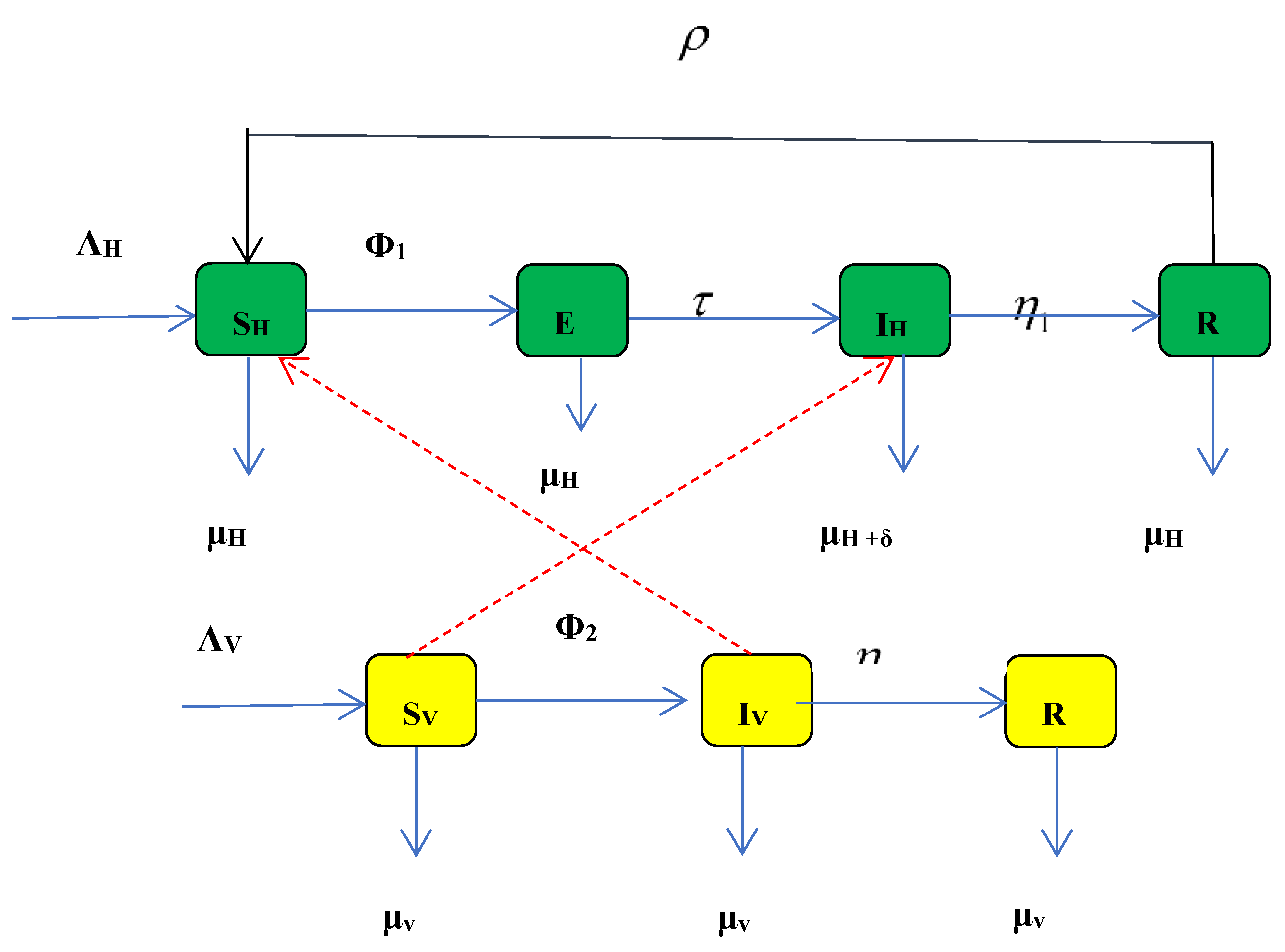
According to the proposed model, the whole system (population), is represented by the letter "N", and has been split into two primary parts: "Nv" and "Nh" for vectors and humans, respectively.
The susceptible, exposed, infected, and recovered human sub-populations (Sh, Eh, Ih, and Rh) are present in ′Nh′, respectively, from this subdivision; similarly, for the vector sub-population, Nv , we have susceptible, infected, and recovered, (Sv, Iv, and Rv), assuming that the domestic animals can recover from the disease with an appropriate control techniques .
Additionally, the recruitment /immigration of humans and vectors into the population in question occurs through birth or immigration at rates of
and
, respectively. Humans and vectors contract the anthrax virus through contact with diseased animals or consumption of tainted dairy and animal products containing
Bacillus anthracis, at forced or saturated rates of infection,
and
The effective contact rates that can result in infection and saturation factor are represented by β1, β2, β3, and , respectively.
The results of this study show that the saturation rates and infection forces in (9) and (10) above predict the behavioral change in the model when Ih and Iv grow very big in the system as well as their repressive effects when simulated. This is the reason this model has taken into account the specific saturation incidence rate.
In this model, we have also taken into account the possibility that individuals may lose their immunity, making them susceptible to infection again at the rate ρ after receiving treatment, with a recovery rate of η. However, in severe cases of anthrax sickness, people may pass away at a rate of δ because to the virus's virulence.
3.2. The Anthrax Model’s Equations
The set of time fractional differential equations designed to describe the dynamics of the disease is basically on the descriptions and assumptions of the above Model (
Figure 1).
Here
, for 0
< α ≤ 1 in the sense of Caputo Fractional derivative of order
α
Table 1.
.
| Parameters |
Description |
SH
EH
IH
RH
SV
IV
RV
|
human Susceptible
human Exposed
human Infected
human Recover
vector Susceptible
Infected vector
Recovered vector
Immigration/recruitment rate for human
Immigration/recruitment rate for vector
Force of infection for human(saturation function)
Force of infection for vector (saturation function)
Loss of immunity human
Natural death rate for human
Natural death rate for vector
Rate of Progression from exposed to infected class of human
Rate of Progression from infected to recovery class of human
Rate of Progression from infected to recovery class of vector
The rate of effective contact between vector and humans
rate of effective contact between domestic vector and Bacillus anthracis
Rate of contact leading to infection for the vector
disease induced death |
3.3. Mathematical Analysis of the Model
3.3.1. Existence and Uniqueness of the Model Solution
To demonstrate the uniqueness and existence of solutions to the system (11), Lemma (2.6.3) as it has been given above is required, which is given as;
For U ∈ C[a, b] and ∈ (0, b] let 0 < α ≤ 1, hence we
(a) For , ∀ t ∈ (0, b) then the function u is increasing
(b) For , ∀ t ∈ (0, b) then the function u is decreasing.
The proof of the above lemma is direct consequence of lemma (2.6.2) which is the generalized Mean Value Theorem.
3.3.2. Boundedness and Positivity of the Model
In this section, we verify and ascertain if our proposed model is epidemically and mathematically accurate. Moreover, each compartment's solutions be non-negative (positive). The whole vector population is represented by NV= SV + IV + RV, while the total human system is represented by NH = SH + EH + IH + RH.
From (12) we can conclude that for both Human and Vector compartment we have
( = 0 for both human and vector compartment) i.e the disease induced death in order to achieve (13)
Theorem 3.3.3. Let and be the solution to the Anthrax Fractional model equation (11) in an epidemiology viable area
Proof
With the Laplace transform applied on both sides of (13), (both human and Vector) and using the Definition 2.6, (7) we have
After little modifications and Rearrangement on (15) we have
After considerable simplification and application of the Laplace inverse transform and (Lemma 2.6.1) i.e (8) as given earlier on (16), the following was derived
applying (17) with lemma 2.5.1, as
t tends to
∞ the following was obtained
Thus, every solution for systems (11) is included inside the set , hence is bounded for both Human
And vector population.
Hence, from Equation (13) to (18), we have been able to verified that the solutions for the various compartments are bounded and that the model is well-posed both mathematically and epidemiologically.
This ends the proof.□
3.3.4. Positivity
For all time t > 0, the Fractional order model's solution in system (11) with positive initial conditions will continue to be positive and non-negative
Proof
Using the Mittag-Leffter function also known as two parameter function (5) and (6)
Replacing
with our population
and
respectively and separately, where
and
Neglecting the higher terms
We have also been able to verify that the model is positive for time (t) based on equations of the model (11)
This ends the proof. □
3.4. Presence of the Disease-Free Equilibrium Points
The term "disease-free system (equilibrum) (DFE) points" refers to stable-state solutions when the population as a whole becomes immune to anthrax infection.
Hence system (18) becomes
which yields
Therefore the disease free equilibrium point for both Human and Vector population is
(25) Is the DFE point for the system.
3.5. Computation of the R0 (Reproduction Number) of the Human-Vector Model
In an epidemic model, the Ro is an essential concept. This figure indicates the typical number of later infections in the Exposed section of the population among all individuals in a population that is fully susceptible and infected by an infectious person already in the infected compartment. Similarly Ro is a crucial metric that tells us whether or not a disease will spread over the population. The "next generation matrix method" will be used in order to calculate it.
In this case,
V is the linear system of additional transfer terms with infection, and
F is the linear system matrix of the new infection. Consequently, the model's fundamental reproduction number is obtained using
, where
is the dominant eigenvalue of
which yields
, here
is the combination of both compartment (Human and Vector)
The possibility that human will survive the exposed stage before becoming infectious is And similarly, Is the possibility also that vector population might endure the exposed stage before becoming infectious.
Where is the median duration of the infectious time on human population
3.6. Local Stability Analysis of Anthrax at (DFE)
After establishing the existence of a disease-free equilibrium for our proposed model, we will now conduct stability analyses on the system to infer its long-term effects regarding whether or not it is stable.
Theorem 1:
If all the population's Jacobian eigenvalues are non-positive(negative) real values, then our system's DFE is asymptotically stable.
Proof: in order to establish the theorem above, we calculate the Jacobian of the model’s system (11) at its Disease free equilibrium (DFE)
The jacobian computation goes thus
Now at disease free equilibrium and introducing our 7 by 7 identity matrix we have
After steadily solving and necessary simplifications of the 7 by 7 jacobian matrix we obtain the following values as our Eigen values;
It is evident that every one of our eigenvalues for the seven by seven dimensional systems is negative (λ1, λ2, λ3, λ4,..., λ7 < 0), indicating that the local stability of the system DFE exists.
3.7. Global Stability (GAS) of the Anthrax Model at DFE
Theorem 2 : The Anthrax free system of model (11) is globally stable asymptotically in the epidemiological viable region if RHV < 1and unstable otherwise
Considering (34), we set the rate of changes of (34) to zero, consequently, we have that
which is the necessary for Anthrax free equilibrum.
Now let and , where K denote the set of uninfected and J denote the set of infected, we say that the point is Global Asymptotical Stable (GAS) if ,
And the subsequent conditions holds;
, then is GAS, here, which is the integer order of our fractional model, we assume our
There exist such that for every
Proof of the first conditions
for
we have
It’s evident that the first condition holds, Hence is satisfied
Mini-proof
, using the method of
, as we have that , this also goes for vector population
as
Conveying the global convergence of
This complete the mini-proof
Proof of Second condition
could also be written in the form
We need to show that in (37) the vector Matrix C is given as
, where
is the stable state matrix which establish the second condition of the GAS
Which completes the proof. □
3.8. Analysis of the Sensitivity of Parameters of Anthrax-Vector Model
The main goal of sensitivity analysis is to ascertain how each variable affects the rate of reproduction. This aids in determining the parameters that have a significant influence on R
HV. In order to determine whether or not immunization, mortality, and infection treatment could aid in the management or eradication of the disease in the system, the basic reproduction rate is often examined [
38]. This technique is widely employed to test the resilience of model assumptions to variable values. The examination of the model's reproduction number R
HV, which looks for variance and the impact of changing a parameter on R
HV, will be carried out.
Definition: The normalised forward sensitivity index of a variable a, is given by:
Which depends on the differentiability of parameter b
We would now have to carry out the analysis of the fundamental reproduction number specifically on some key parameters that makes up the reproduction number and with regard to parameters that makes up our model
The sensitivity index for
and every other parameters will be computed for
By analyzing the derivatives in (41)
By this we obtain the sensitivity index for
In the same vein we will use this method for all other parameters that makes up the reproduction number in other get there sensitivity index, though not all the parameters have positive values according to
Table 2
3.8.1. Interpretation of RHV Sensitivity Indices
The value of Rhv in epidemiological models indicates how easily a disease may spread throughout the community. By calculating the sensitivity indices of Rhv with regard to the model's parameter values, we will be able to calculate the decrease in infection caused by the diseases. The contribution of each parameter to the dynamics of the diseases is determined by the sensitivity indices. We determine the sensitivity of RHV to each parameter in the model (11) taking into account all of the system's properties.
Table 2 lists the sensitivity indices of Rhv for each system parameter in model (11).
A thorough sensitivity analysis of RHV revealed that a rise in would result in a reduction in RHV. Furthermore, if were to decrease, RHV would rise. Moreover, for a rise in RHV implies that there is an increase in the values of , and a fall in RHV would result from a decrease in those values respectively
3.9. Numerical Simulation
We have reviewed, investigated, and evaluated the analytical/simulated outcomes of the Anthrax-vector interactive model in this section. This has been done in order to confirm the results of our sensitivity analysis, to validate our theoretical conclusions, and to investigate, evaluate, and elucidate the dynamic behavior of the population being considered. We have simulated the full model and individual compartments using the MATLAB (software) program, taking into account the initial circumstances (state variable values) and changing a few significant model parameters.
Table 3 presents the values, dimensions, and origins of these parameters.
While some of these parameters were based on reasonable estimations and assumptions, the majority of them were clinical facts that were taken from reputable literature.
Figure 1.
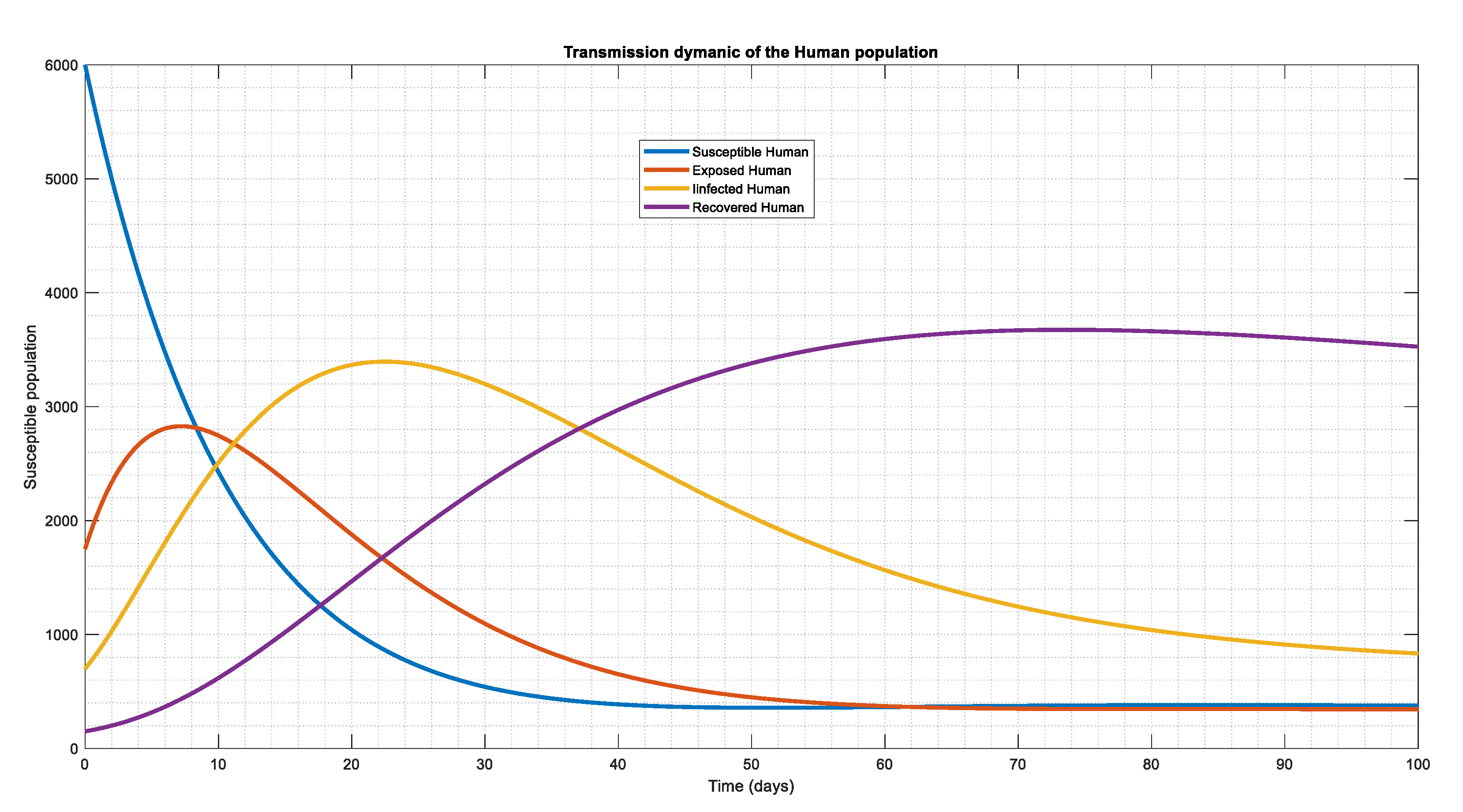
The human population dynamical behavior with, , , . , , = 0.30, demonstrating the coexistence of the compartment and driving the system's tendency toward an endemic condition.
Figure 1.
The human population dynamical behavior with, , , . , , = 0.30, demonstrating the coexistence of the compartment and driving the system's tendency toward an endemic condition.
4. Discussion
Using the values on
Table 3 and
Table 4 alongside with the parameters, we have simulated the model. We now must adjust a few of these factors on the above table in order to see the changes (behavior) in our model.
Using the initial conditions and parameter values from
Table 3 and
Table 4, the merged graphs of the whole human population are shown in
Figure 1. The section of exposed and infected humans increases during the starting phase (instantaneous time), however over time, both the exposed and the infected reach a stable state as a result of the system's dynamic behavior, as shown in
Figure 1. The human population begins to recover after a while, however during the early phase, the whole system tends to be vulnerable, demonstrating the mathematical epidemiology of our model (which tends towards endemic condition)
The dynamic behavior of each human compartment is depicted in
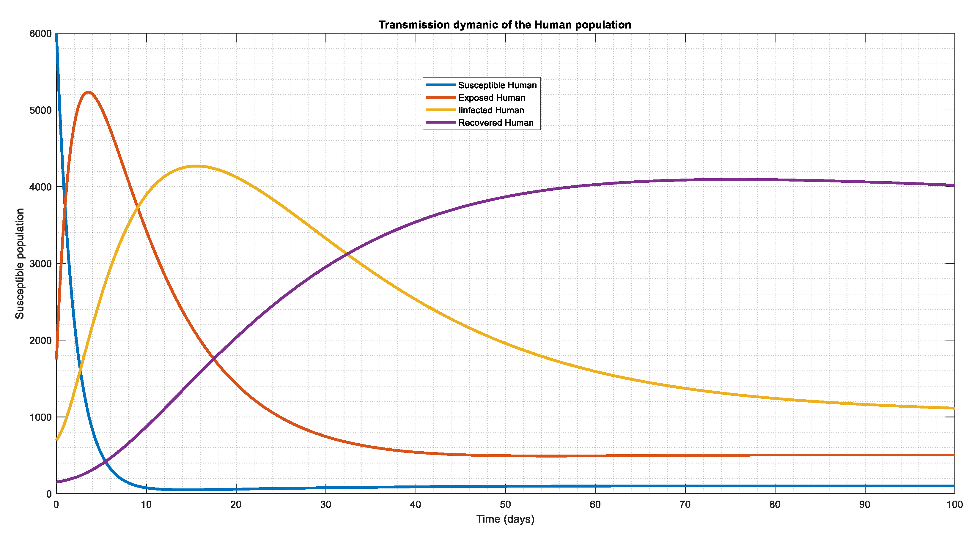
Figure 2 when the infection force
and the human immigration rate
are varied. By changing these parameters, we found that people become increasingly exposed to the virus and become sick; the population of susceptible people declines dramatically and abruptly in less than ten (10) days compared to figure 1, although people generally recover within ninety days. These all demonstrate how the system is approaching an endemic condition since every compartment coexists in it.
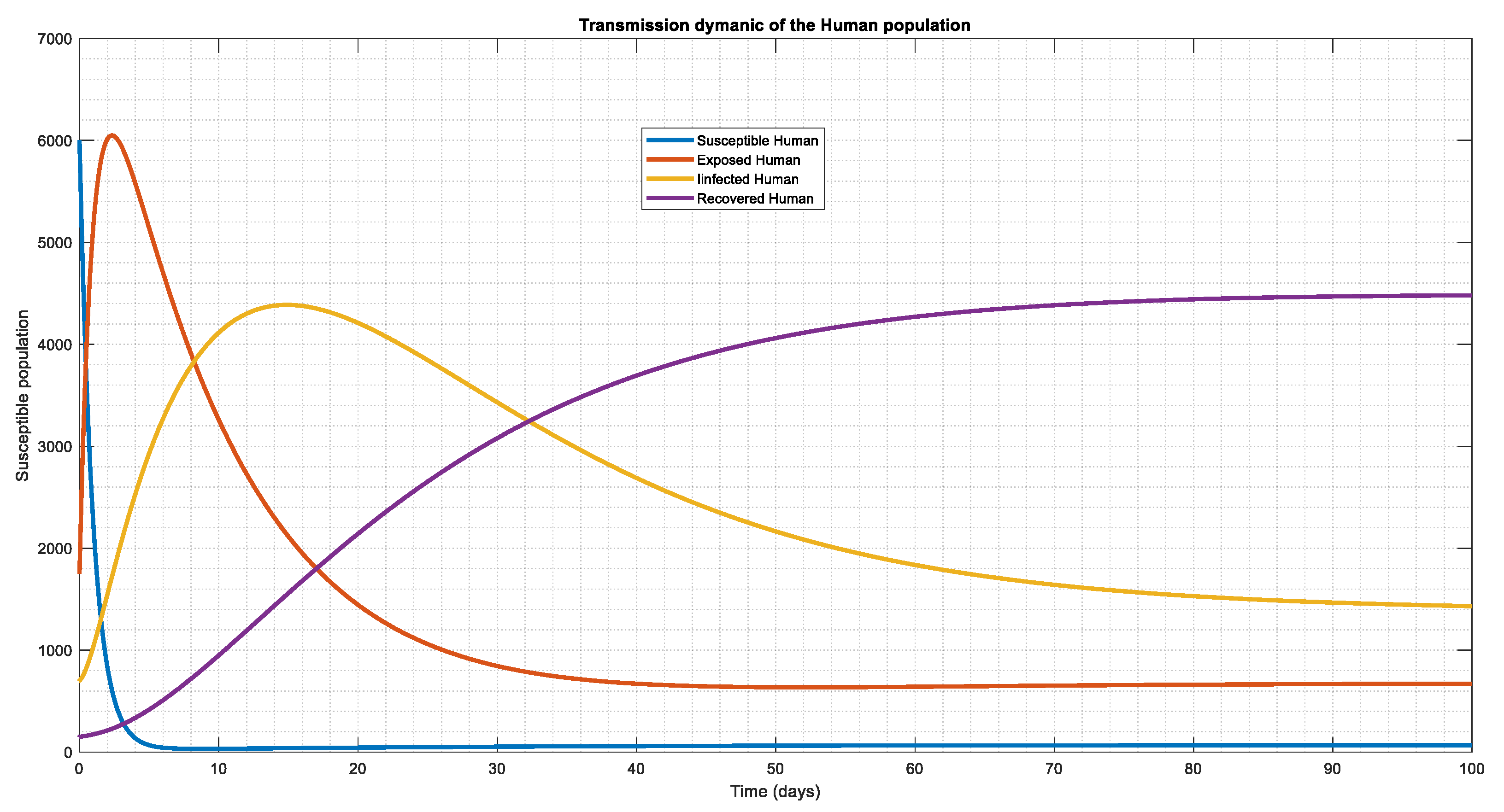
The system's behavior when the immigration rate is raised and the infection force is
is unity as seen in
Figure 3. the human system is exposed very quickly at one point in time again demonstrating the mathematical epidemiology of our model and after a month (30days), the infected human population likewise grows at steady rate, leading to a sharp decline in the susceptible population below 10 days.
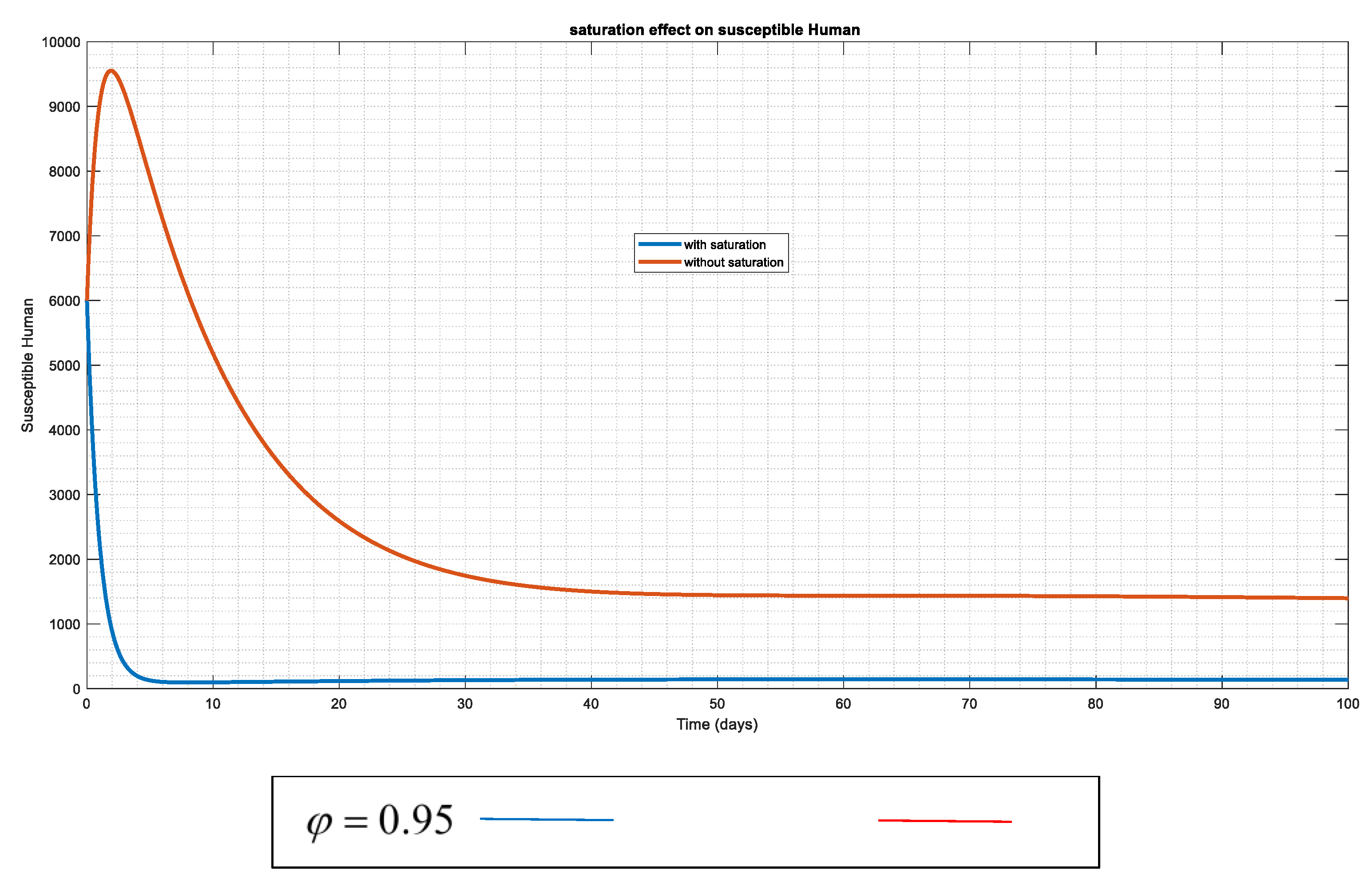
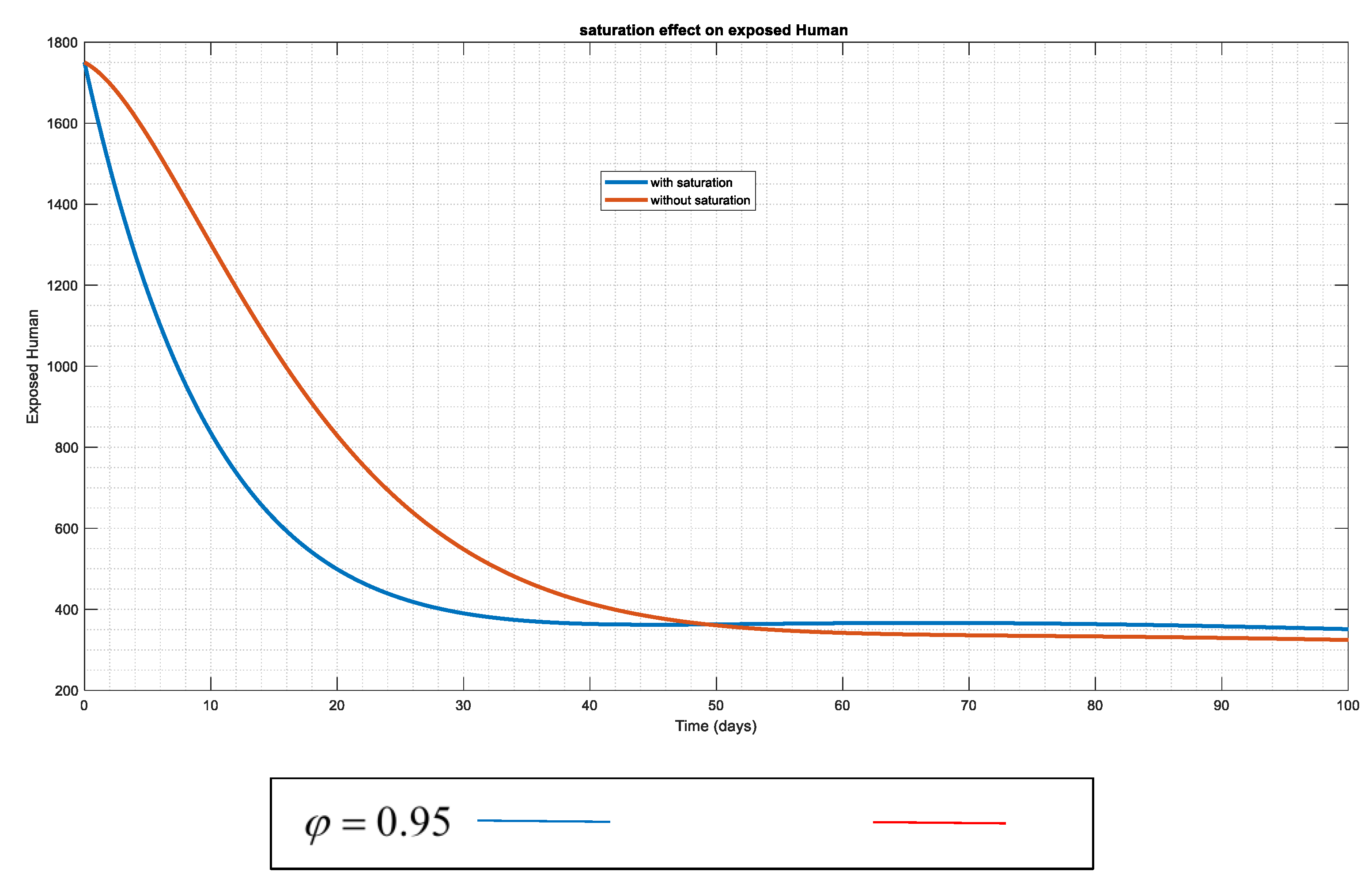
To confirm and substantiate the impact of the saturation in this suggested framework (model),
Figure 4 and
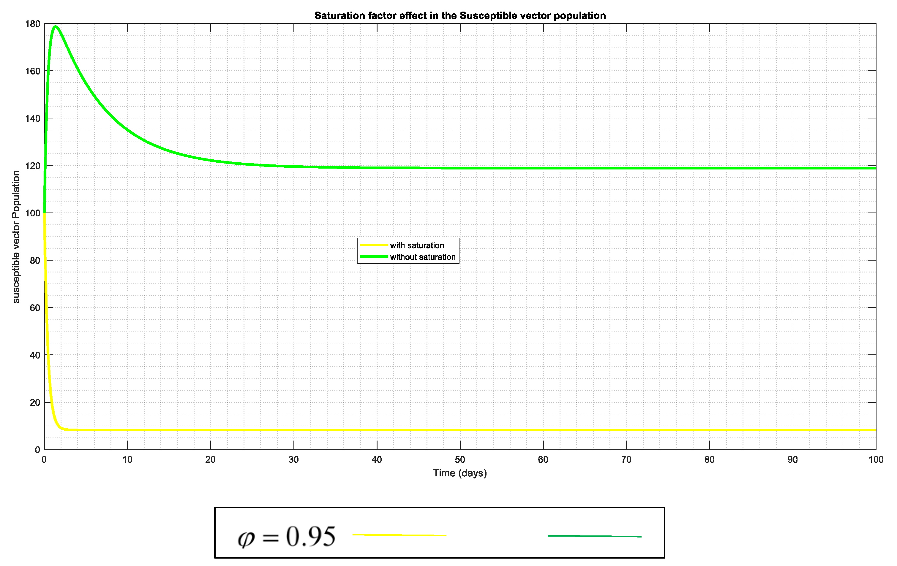
Figure 5 have been utilized. The dynamic of the exposed and susceptible humans reveals that when "saturation" occurs, the populations of these humans are drastically reduced, leading the system to approach stability (DFE). This could be caused by various control measures, such as hunting wild animals with the infection in the instance of the vector population as seen in (
Figure 12), immune response to the infection, or early management of medications like vaccination (and other necessary interventions) in both populations
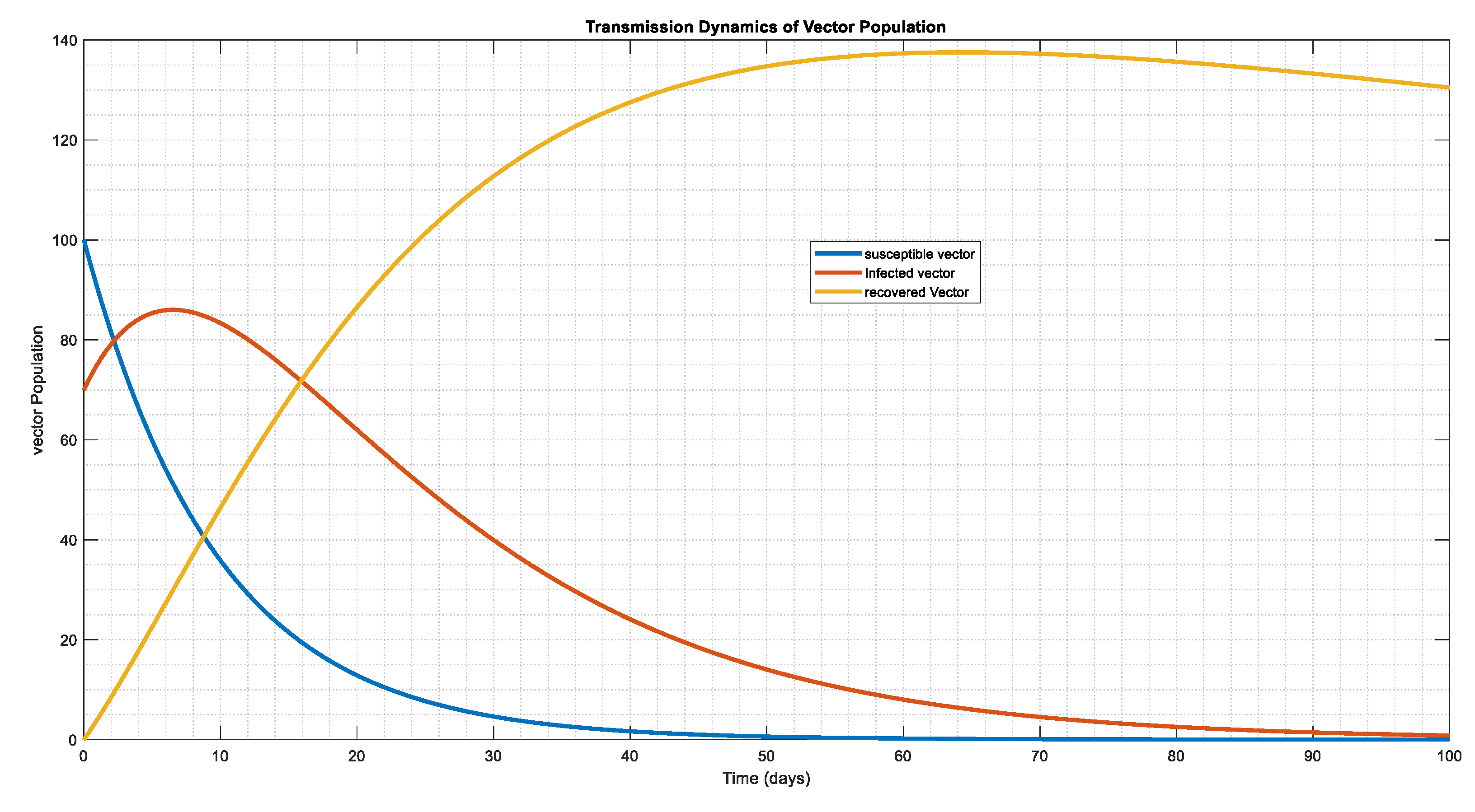
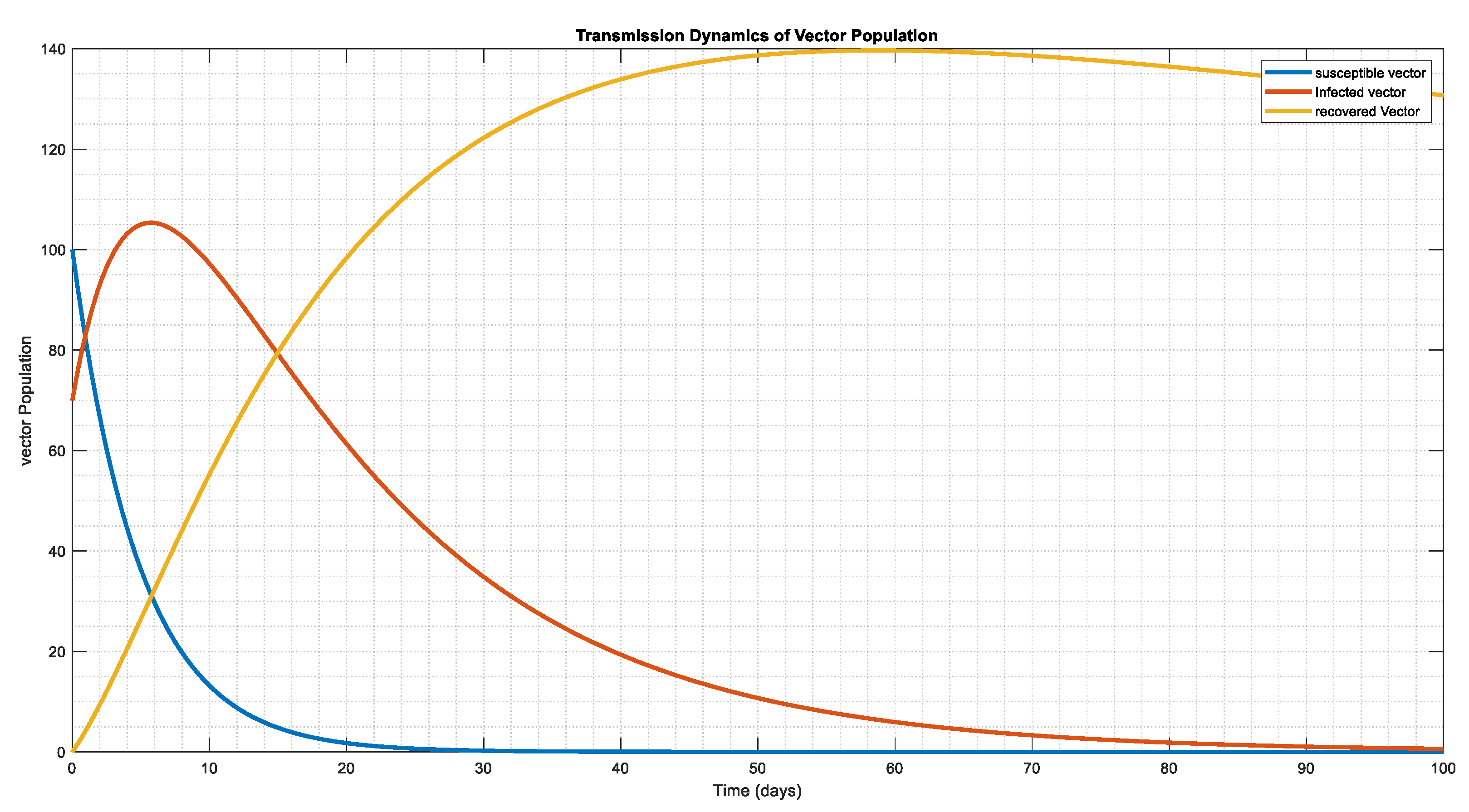
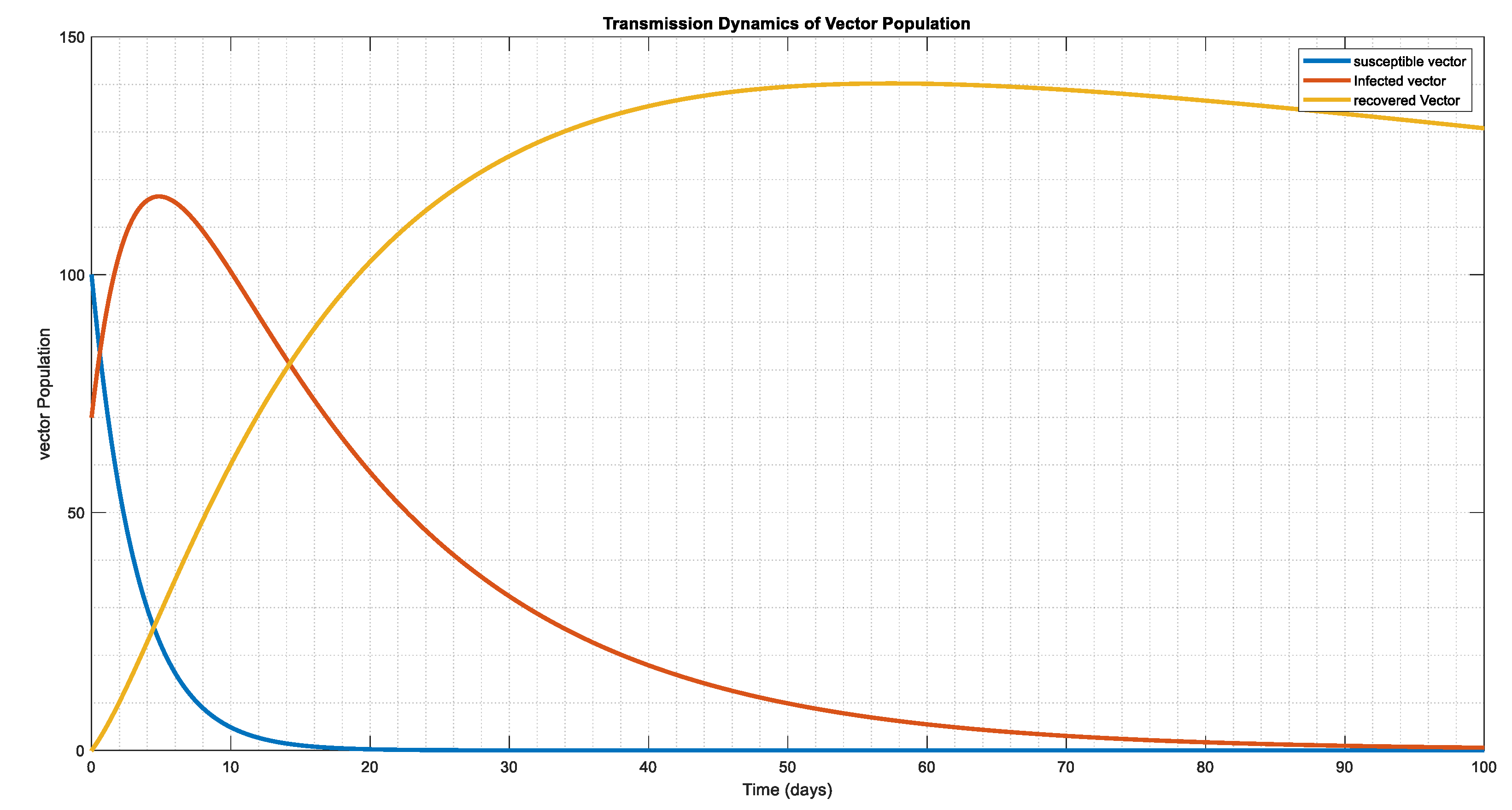
The vector system's dynamic behavior in
Figure 7,
Figure 8 and
Figure 9, in relation to the starting conditions and parameter figures on
Table 3 and
Table 4, where we double and triple the infection force for
Figure 8 and
Figure 9, respectively. This indicates that the vector tends to be exposed at a single moment, resulting in infection in lesser period 30, 20, and 10 days, apart, however the population of the infected eventually reaches a stability state, and the population of the susceptible disappear over time, leaving only the population of the infected in the system.
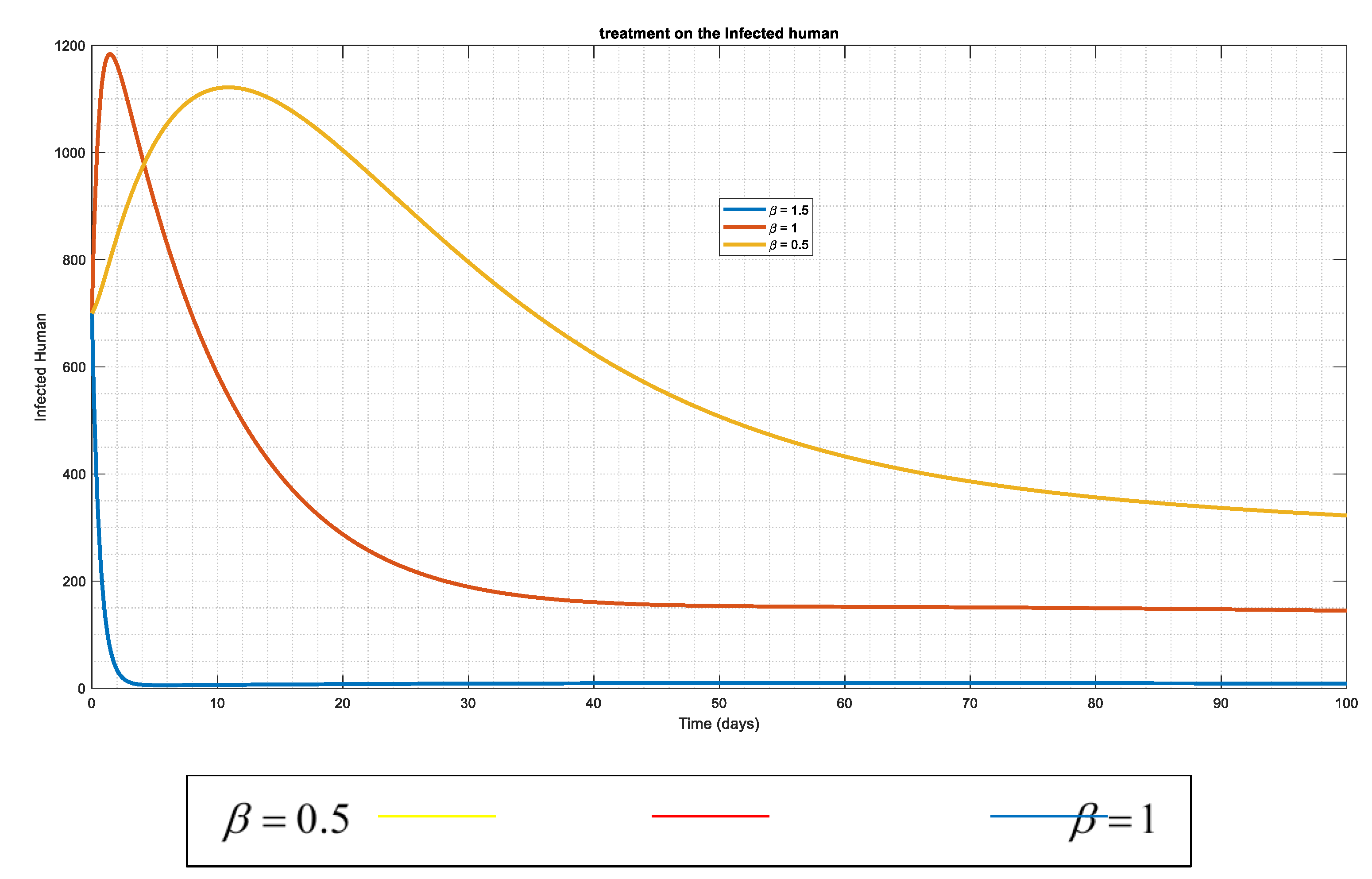
Figure 6: presents a control strategy that aims to flattens the spread of disease among the infected human population. The therapy is modified by doubling and tripling its effect over time, hence the system tends towards DFE state. That is Disease free system.
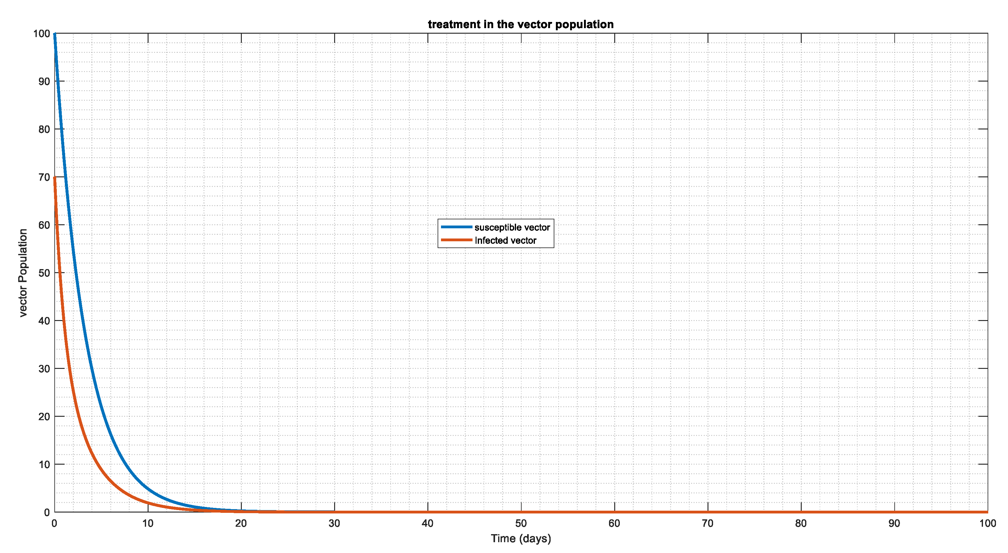
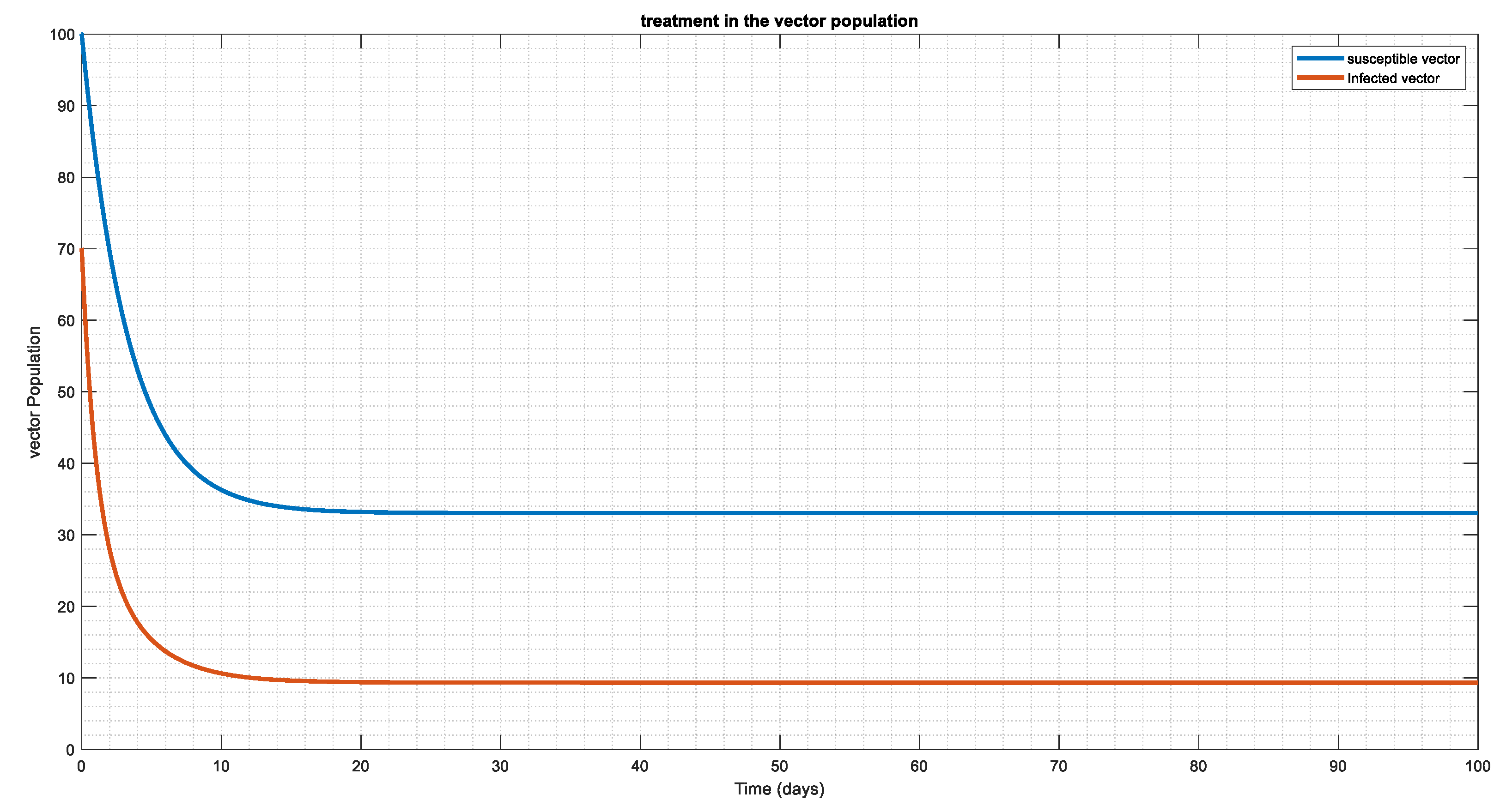
Since vectors are the carriers of the disease, we aim to minimize the rate at which humans will contract it by introducing an effective control plan in susceptible vector and infected vector populations (
Figure 10 and
Figure 11). Additionally,
Figure 11 illustrates that, regardless of the number of susceptible vector populations, an effective control plan will eventually cause the population to reach a disease-free system.
Figure 2.
Here the recruitment was increased
and the force of infection
while other parameters remain the same which also shows that all compartment co-exist causing the population to approach endemic state, but one thing that is noticeable here is that the susceptible shows a sharp decline compared to
Figure 1.
Figure 3.
Similarly the recruitment rate was increased the third time i.e , again we notice a sharp decline in the susceptible region which will hence affect the exposed and the infected causing the whole population to tends to toward endemic state.
Figure 3.
Similarly the recruitment rate was increased the third time i.e , again we notice a sharp decline in the susceptible region which will hence affect the exposed and the infected causing the whole population to tends to toward endemic state.
Figure 4.
The susceptible human's changing effects both with and without the "saturation factor" This indicates that the introduction of saturation lowers the incidence of human vulnerability to anthrax.
Figure 4.
The susceptible human's changing effects both with and without the "saturation factor" This indicates that the introduction of saturation lowers the incidence of human vulnerability to anthrax.
Figure 5.
The Exposed human's changing effects both with and without the "saturation factor" This indicates that the introduction of saturation lowers the incidence of exposed compartment to anthrax.
Figure 5.
The Exposed human's changing effects both with and without the "saturation factor" This indicates that the introduction of saturation lowers the incidence of exposed compartment to anthrax.
Figure 6.
The effect of increasing the rate of treatment for infected individuals by vaccination administration (along with other essential treatments) demonstrates how early antiviral medication administration and implementation may significantly reduce the population inside the infected compartment.
Figure 7.
The dynamical behavior of vector population with , , , showing how the compartment co-exist and which in essence the vector population tends to endemic state.
Figure 7.
The dynamical behavior of vector population with , , , showing how the compartment co-exist and which in essence the vector population tends to endemic state.
Figure 8.
In the above figure above , that is we doubled the incidence figure, while other parameter remain same, we notice a sharp decline in the susceptible class which changes the behavior of the population as whole.
Figure 8.
In the above figure above , that is we doubled the incidence figure, while other parameter remain same, we notice a sharp decline in the susceptible class which changes the behavior of the population as whole.
Figure 9.
In the above figure above the incidence figure was tripled in other to see how the population,
, while other parameter remain same, we notice a sharp decline in the susceptible class which changes the behavior of the population as whole.
=10, while other parameters remain the same, we noticed that irrespective of the susceptible number to the system with effective control strategies the vector population will still attain DFE.
Figure 10.
Here we try to introduce effective control plan to vector population with =0.005, =0.3 the figure above showing that the vector population can approach disease free equilibrium (DFE), especially the susceptible and infected population.
Figure 10.
Here we try to introduce effective control plan to vector population with =0.005, =0.3 the figure above showing that the vector population can approach disease free equilibrium (DFE), especially the susceptible and infected population.
Figure 11.
In the figure above the vector recruitment rate was increased to
Figure 11.
In the figure above the vector recruitment rate was increased to
Figure 12.
The susceptible vector changing effects both with and without the "saturation factor" This indicates that the introduction of saturation lowers the incidence of vector vulnerability to anthrax.
Figure 12.
The susceptible vector changing effects both with and without the "saturation factor" This indicates that the introduction of saturation lowers the incidence of vector vulnerability to anthrax.
