Preprint
Article

Instantaneous Material Classification Using a Polarization-Diverse RMCW LIDAR

Altmetrics

Downloads

125

Views

53

Comments

0

A peer-reviewed article of this preprint also exists.

Submitted:

09 March 2024

Posted:

14 March 2024

You are already at the latest version

Alerts
Abstract
Light detection and ranging (LIDAR) sensors using a polarization-diverse receiver are able to capture polarimetric information about the target under measurement. This information can be used in a classifier to make an instantaneous assessment of the type of material present, enabling a shot-by-shot prediction of the material type and distance to the target.
Keywords: 
Subject: Physical Sciences  -   Optics and Photonics

1. Introduction

Light detection and ranging (LIDAR) is a critical sensor used by autonomous vehicles, as it provides a dense pointcloud with exceptional angular resolution, enabling the ability to provide mapping as well as detection and classification of moving objects in the environment [1]. Each point in the pointcloud is a detection event, where the LIDAR sensor has emitted energy, and received some portion of the reflected energy, using the time delay between these two events to calculate an accurate estimate of distance.
Next-generation LIDAR will use homodyne or coherent detection in the receiver hardware; this approach has several advantages over direct detection systems, such as the ability to instantaneously measure the Doppler velocity of moving targets [1]. This is possible as a homodyne detection system is able to measure the amplitude and phase of the reflected light, which provides the LIDAR sensor with additional information about the objects in the environment. In contrast, direct detection systems are sensitive to the intensity of the received signal, which is sufficient for ranging, but cannot measure the Doppler shift from a moving object.
Autonomous vehicles use sensors to understand the world around them, and in many applications, understanding the physical properties of the environment can greatly improve their functionality, such as when a sensor can classify a detection by the material type or structure; we call this ability “material classification”. This capability has been demonstrated in several autonomous applications, such as using feedback from force sensors in robotic excavators [2], using robotic arms and optical sensors in recycling plants [3], or capturing infra-red (IR) spectra of biomass on a production line to understand the composition of the feedstock [4]. Other methods of active sensing for material classification have been demonstrated with thermal sensors [5] as well as millimeter-wave vibrometry [6].
Material classification using laser sensors has shown tremendous potential; compared to camera-based methods, which are lighting dependent, and rely on visible color [7], lasers provide a stimulus to the material, and then the sensor receiver records the response. Typically, the reflection from an objects is treated as an ideal Lambertian surface, which is a diffuse reflector, but real-world objects have complicated behaviour which can be characterized and used to identify materials [8]. Kirchner et al. demonstrated the ability to classify 5 materials using the depth error over angle and intensity from a commercial laser rangefinder [9]. Similarly, intensity histograms have been used in aerial LIDAR to classify different types of forest, as well as surfaces, such as water, gravel, low vegetation, using a simple decision tree classifier [10].
Several authors have looked at using off-the-shelf time-of-flight (ToF) cameras to exploit depth errors for classifying materials in an image, independent of the material color [7,11]; Tanaka et al. also demonstrated that the accuracy could be greatly improved from 55.0% to 89.9% by sweeping the modulation frequency as well [7].
The wavelength response of objects in the environment is highly effective method of discriminating materials, has been extensively utilized as the enormous field of spectroscopy, and is demonstrated in diverse methods, such as hyperspectral cameras for material identification [12,13], optical absorbance sensors for detecting heavy metals in water[7], and many others. For the purpose of this article, we will focus on single wavelength LIDAR systems.
Polarization is an additional property of light, which describes the orientation of the oscillation of an electromagnetic wave; when reflected back from an object, the polarization state may change in a manner that is related to the physical structure of the surface of that object [14]. This insight led to investigations into how to leverage polarization LIDAR to measure depolarization of returns from different particles. Simply stated, Mie scattering from spherical particles results in the reflected light maintaining the same polarization as the transmit beam; when the particles are non-spherical, some proportion of the reflected light is depolarized [14]. In a specific example, Sassen et al. demonstrated using polarization LIDAR to measure the ash size distribution from a volcanic eruption off the coast of Alaska [15]. Alternatively, simply augmenting LIDAR with a passive polarimetric sensor was shown to provide over 90% accuracy in classifying materials, even in low SNR conditions [16]; in this article, the authors demonstrate the large improvement in classification accuracy by combining polarization with the LIDAR information.
Using polarization-coded LIDAR, Nunes-Pereira et al. demonstrated that polarization could be effectively used in classification of common materials observed in operational domains for autonomous vehicles, and to understand the effect, conducted extensive examinations of the polarization-dependent reflectance of materials, then used optical coherence tomography (OCT) to determine the material cross-section of automotive car paints [17]. In order to reconstruct the degree of polarization, the authors used a pulsed ToF LIDAR and placed a linear polarizer in front of the optics. To capture the orthogonal polarization, they rotated the polarizer and repeated the capture, synthesizing a material-coded pointcloud by processing both polarizations.
In this paper, we demonstrate a polarization-diverse LIDAR using random modulated continuous wave (RMCW) ranging with a polarization-diverse homodyne receiver,enabling material classification on an instantaneous shot-by-shot basis, only using the data acquired by the LIDAR sensor during the acquisition time. Our polarization-diverse receiver uses an integrated photonic chip to produce received signals for ranging and for calculating the polarization parameters required by our machine learning model. To our knowledge, this is the first polarization-diverse RMCW LIDAR system that has been demonstrated to perform instantaneous material classification.

2. Theory

2.1. Random Modulated Continuous Wave (RMCW) Ranging

RMCW ranging is a technique that avoids using narrow, high peak power pulses by spreading the same energy into a low peak power series of pulses, coded by a pseudorandom sequence, and was first described by Takeuchi et al. in 1983[18]. When the received signal is digitized, it is simply correlated with the reference sequence, resulting in a correlation peak corresponding to the delay of the signal, which can be used to calculated the distance to target.
The polarization-diverse homodyne receiver is a much more complex system than the direct-detection scheme shown by Takeuchi et al., as we have four differential signals to digitize and combine, corresponding to X- and Y-polarizations, as well as the in-phase (I) and quadrature (Q) components; a thorough discussion of these devices and how polarization is recovered is shown by Roudas et al. [19].
Additionally, recovering our RMCW signal in a homodyne receiver is challenging due to the phase fluctuations of the laser source - while this can be ameliorated by using a narrow-linewidth laser, it is useful to have a system that is insensitive to laser linewidth, as this increases the types of lasers available for RMCW ranging. We provide a detailed discussion of detecting homodyne RMCW LIDAR signals in [20].
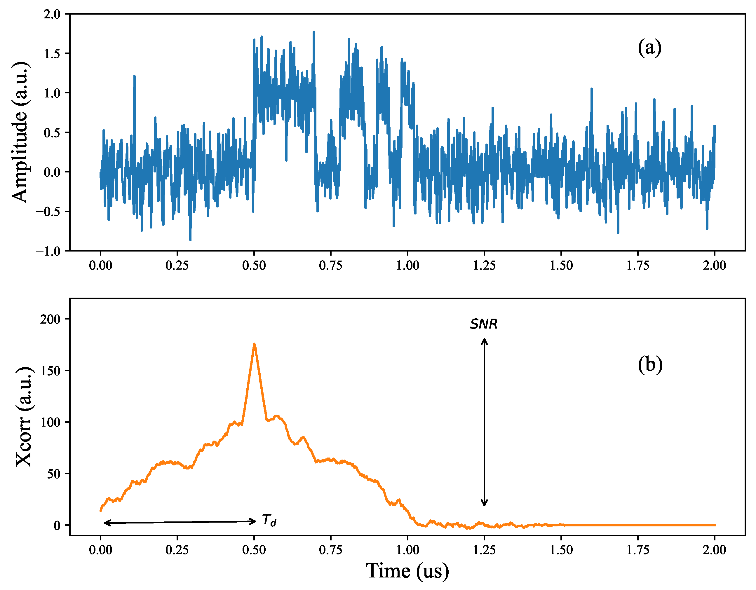
As an example, we show a numerically generated example of an RMCW time domain signal converted to the correlation domain; we generated a Barker-13 code and delayed it by 0.5 μ s in an acquisition window of 2.0 μ s . We included additive gaussian white noise (AWGN) to introduce noise to the received signal, shown in Figure 1(a). After correlating with the ideal reference Barker-13 sequence, we get a correlation signal in Figure 1(b), where the correlation peak corresponds to the time delay from the return signal, T d . The distance to the target is then simply
d T = T d · c 2 ,
where c is the speed of light. The signal-to-noise ratio (SNR) is calculated as
S N R ( d B ) = 10 log 10 X P 3 σ ,
where X P is the correlation peak height, and σ is the standard deviation of the noise fluctuations in the correlation domain. As shown in Figure 1(b), the correlation peak has quite a lot of structure outside of the main peak; this is due to the length of the Barker sequence relative to the overall acquisition time. Thus, to calculate the noise variance in σ it is important to exclude any samples that have residual correlation energy in them - for example, we use the last 200 samples to calculate σ .

2.2. Stokes Parameters

The in-phase and quadrature voltage signals are proportional to the eletric field vector in our received optical signal, and we can therefore treat this as a Jones Vector j ( j x , j y ) denoting the polarization of transverse electric field. The zero phase of the received j will be neglected as we don’t have the means to reliably measure a phase difference between transmitted and received light in a way that can isolate the dominant contributions from macroscopic propagation. This is the level of information described by Stokes Parameters [21], a four-element basis for defining polarization states in way that can be measured from optical intensity alone: S 0 as the intensity of the field, and S 1 , S 2 , S 3 as the difference in intensities of the field projected onto different common polarization bases, linear polarizations 0 , 90 then ± 45 and Left- and Right-Circular Polarizations.
S 0 | j | 2 ¯ S 1 | j · ( 1 , 0 ) | 2 ¯ | j · ( 0 , 1 ) | 2 ¯ S 2 | j · ( 1 , 1 ) / 2 | 2 ¯ | j · ( 1 , 1 ) / 2 | 2 ¯ S 3 | j · ( 1 , i ) / 2 | 2 ¯ | j · ( 1 , i ) / 2 | 2 ¯
Here the overline indicates the averaging over a measurement interval, which permits a fraction of power that is depolarized and not contained in S 1 , S 2 , S 3 :
p S 1 2 + S 2 2 + S 3 2 S 0 1
In an RMCW LIDAR system, polarization variation is negligible relative to a sufficiently high sampling rate, however, the polarization variation over a codeword represents a temporal depolarization. The overline in (3) indicates averaging over a codeword.

2.3. Classification strategy

Material classification using LIDAR and polarimetric sensing has been demonstrated with a variety of classifiers, such as SVM, decision trees and neural networks [16], showing good results in accuracy. From this, we conclude that gains from selecting the optimal framework and training strategy are not the focus of this paper; we are investigating the applicability of this method to real-world materials and configurations that would be observed by autonomous vehicles.
Instead, we select a simple feed-forward perceptron model trained and validated using the Predictive modelling tools in JMP 16 [22]. Once we have collected an entire dataset, we use a k-fold cross-validation method, where the number of folds id 5. Thus, the neural network is trained on one portion of the dataset, and then validated on the portion that has not been used for training.
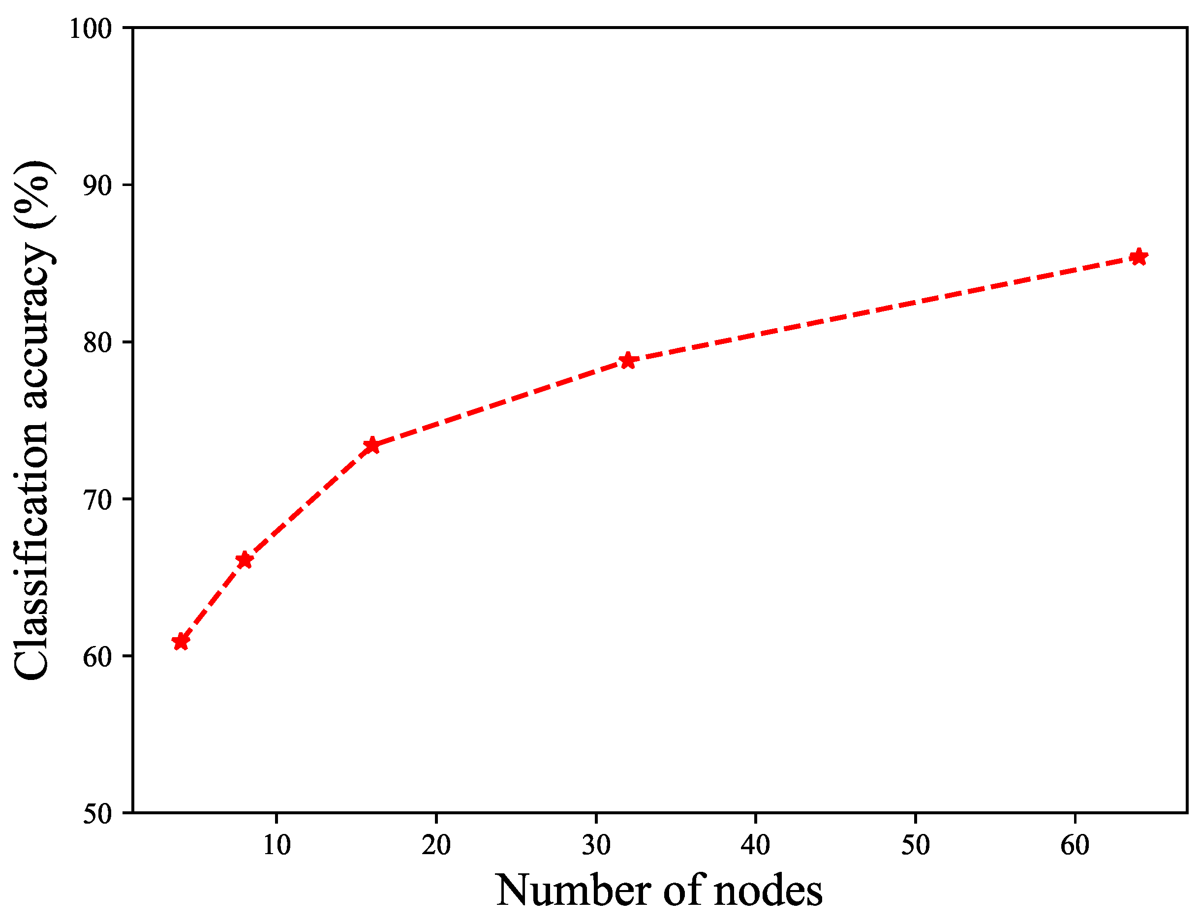
As we will show in Figure 8, increasing the number of nodes in the hidden layer can improve classification accuracy, however we would like to assess the relative performance of this classifier against different sets of materials. With this in mind, we fix our classifier to a feed-forward neural network with a single hidden layer using 64-nodes, and then try to describe results in terms of relative performance.
The presented neural network comprises a perceptron featuring a non-binary output classification. A total of six distinct input nodes are employed in conjunction with 64 hidden nodes. The input nodes consist of the calculated distance to target as in (1), the signal-to-noise (SNR) of the correlation peak as in (2), and the four Stokes parameters calculated from the polarization-diverse receiver, as shown in (3). A hyperbolic tangent activation function is used to facilitate the required non-binary classification. The activation function categorizes materials into output value ranges within the possible -1 to 1 overall output, depending on the number of materials for classification.
The computation of the perceptron output node’s value involves summing the inputs from the hidden nodes, each multiplied by its corresponding synaptic weight. The values of the hidden nodes are similarly calculated by summing the values of the input nodes multiplied by their respective synaptic weights, as shown in [23]. This process is handled via an automated optimizer during the training process and is documented on the JMP website [22].

3. Bi-Directional Optical Sub-Assembly (BOSA)

Recovering polarization from received LIDAR signals can be accomplished with several methods [14,17,24], however, in this work, we use a polarization-diverse homodyne receiver, similar to the work in the digital self-homodyne receiver shown by Puttnam et al. [25], but combining transmit circuit on the same chip as the receive circuit, which we call a bi-directional optical sub-assembly (BOSA).
Within the LiDAR engine, the BOSA is comprised of two primary elements: a receiver (RX) and a transmitter (TX). The transmitter segment encompasses a photonic integrated circuit that produces a local oscillator (LO) signal and an RMCW modulated signal to be sent into the environment. Conversely, the receiver segment incorporates a photonic-integrated polarization-diverse in-phase and quadrature (IQ) receiver. Both of these elements are integrated within a photonic-integrated circuit (PIC), ensuring a compact and efficient design.

3.1. Transmit circuit (TX)

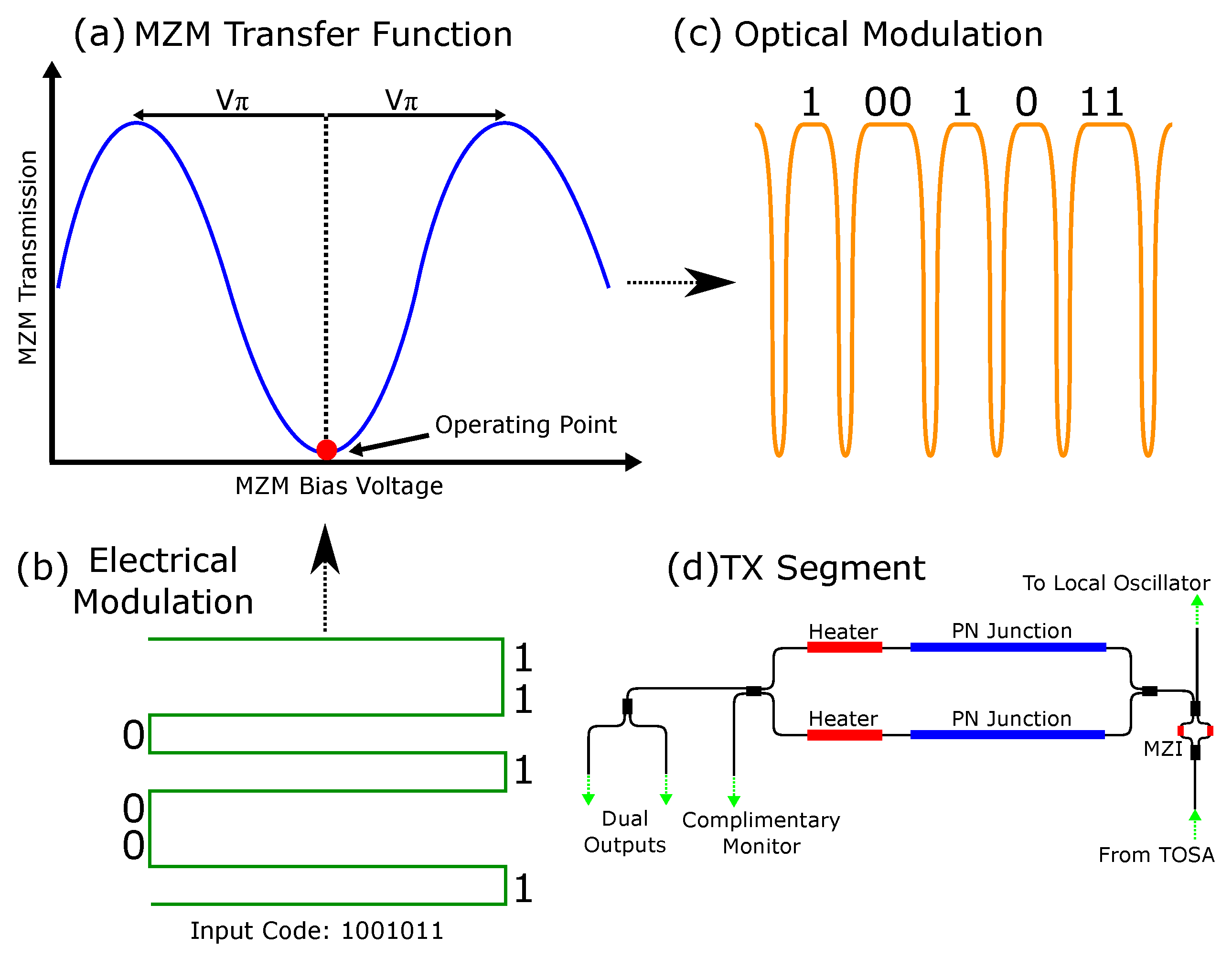
The Tx circuit is shown schematically in Figure 2(d); a laser source is coupling into the TOSA port, and split into local oscillator and signal paths. The local oscillator is used in the receive circuitry for homodyne detection, and the signal path will be encoded with our RMCW modulation before being emitted into the environment. We use a heater-controlled Mach-Zehnder interferometer to provide a tunable split between the two paths.
The Mach-Zehnder Modulator (MZM) plays a pivotal role in transforming the electrical modulation code into optical modulation. This transformation is accomplished by modulating the depletion regions in the PN junctions of the MZM arms, as depicted in Figure 2. To enhance efficiency, a push-pull configuration is employed, effectively doubling the applied drive voltage. This method enables the attainment of the essential 2V π voltage swing for phase modulation, ensuring it is achieved with the least possible power consumption. To ensure that the MZM consistently operates at the required operating point, as depicted in Figure 2(a), thermal heaters are integrated into each arm of the MZM. These heaters enable fine-tuning of the MZM output, thereby maintaining continuous and stable phase modulation.

3.2. Receive Circuit (RX)

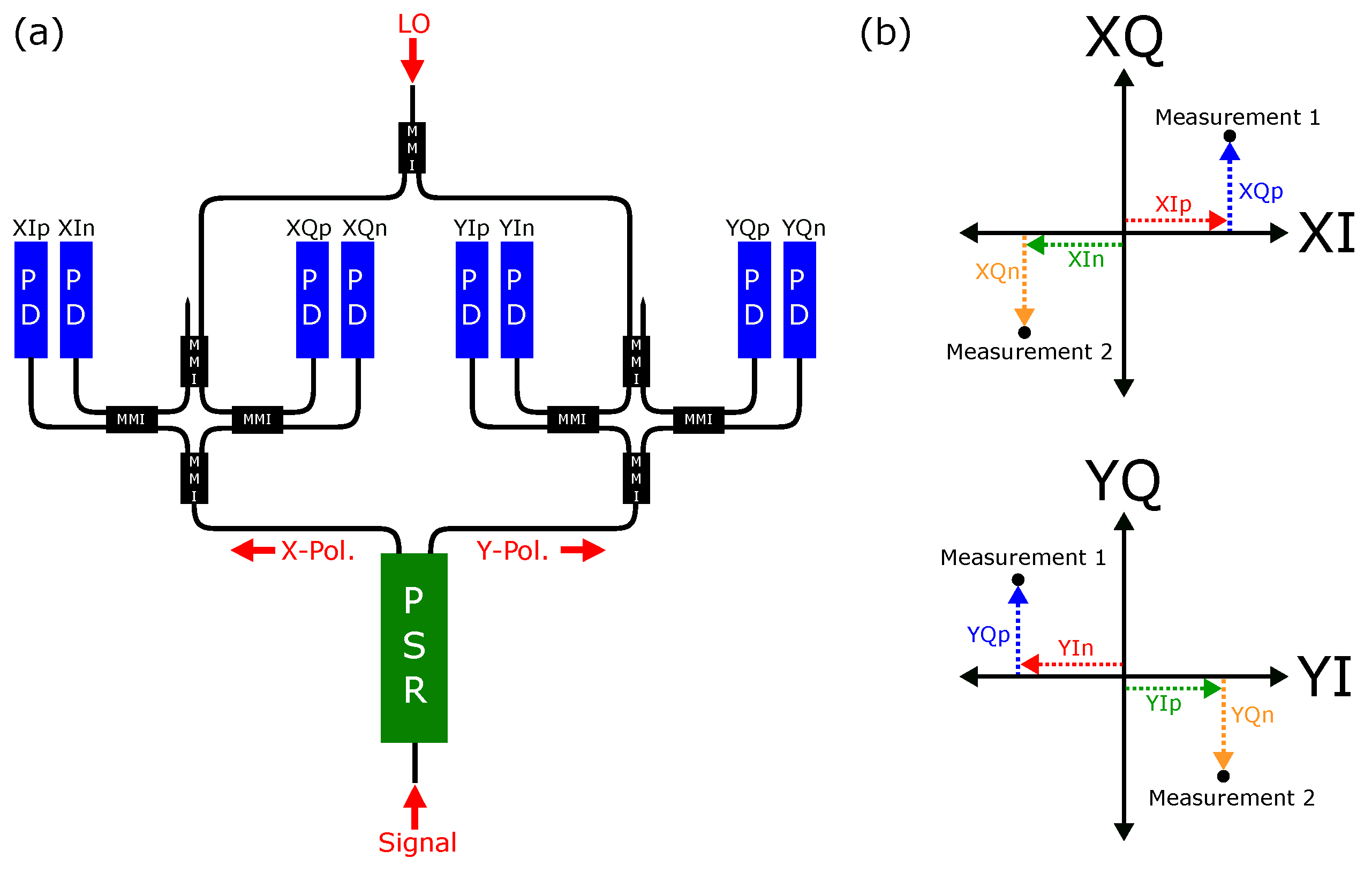
Our ability to detect and classify materials is based on accurate measurement of the polarization state of the received signal, and this Rx circuit in the BOSA is the core component that achieves this functionality. This advanced receiver comprises three principal components: a polarization-splitter-rotator (PSR), 90° hybrids, and photodetectors (PDs), all interconnected via low-loss SiN waveguides within the photonic integrated circuit (PIC), as illustrated in Figure 3(a).
The PSR plays a pivotal role in processing optical inputs with indeterminate TE/TM polarization. It adiabatically transforms the TM component into the fundamental TE mode of the SiN waveguides, while simultaneously transmitting the TE component without alteration. The unaltered TE fraction is hereby referred to as the X-polarization and the adiabatically converted TM fraction is referred to as the Y-polarization. Subsequent to polarization separation, each polarization state is directed to its corresponding 90° hybrid, which consist of four multi-mode interference couplers (MMIs). A 2x2 MMI with an unused input port is employed on the local oscillator (LO) side of the hybrids, whereas the signal input is managed by a 1x2 MMI on the opposite side. This configuration results in a 90° phase difference between the two inputs, essential for the receiver’s capability to process both amplitude and phase information. To convert this optical information into processable electrical information, pairs of vertically-stacked germanium photodiodes are implemented, with their photocurrents subtracted to remove any common-mode noise. The resulting photocurrents generated across the photodiodes are then converted to voltage and amplified through the use of trans-impedance amplifiers (TIAs). The magnitude of the voltages are then utilized to construct IQ constellation diagrams for both X and Y polarizations, as depicted in Figure 3(b).

4. Experimental Setup and Method

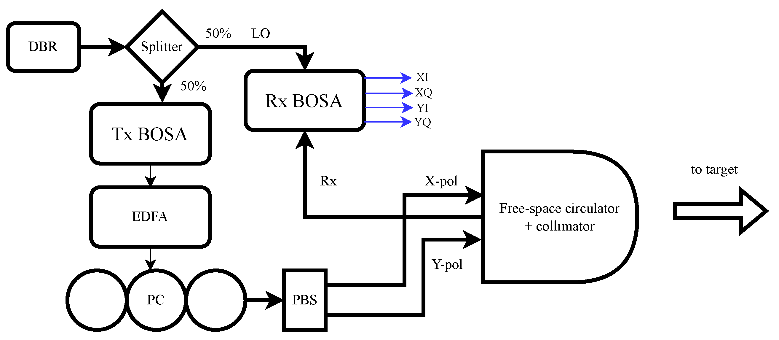
Figure 4 displays the experimental setup used to validate our material classification approach using a single-point RMCW LIDAR system. In our experimental setup, we use a wavelength-tunable DBR laser (Oclaro TL3000), set to 1545.3 nm and with +12 dBm output power. The laser is connected to the input of our custom silicon photonic BOSA, as described in Section 3.1, which modulated the laser signal with a phase-modulated 512-bit Gold code, where the MZM is biased as shown in Figure 2(a). To boost the optical power, we use an erbium-doped fiber amplifier which boosts the transmitted power to +27 dBm.
To control the polarization of the transmitted beam, we connect a fiber polarization controller to the output of the EDFA, and the align the polarization to be 45°linear relative to the input of the polarization beam splitter (PBS). Thus, we have equal power in both X- and Y-polarizations in separate fibers, which are assembled together into a fiber array. As part of our design of experiments, we would like to vary the transmitted polarization, and by connecting/disconnecting the inputs of the PBS, we are able to create roughly 0°, 45°, and 90°linear polarizations.
The optical fiber array is used to closely position parallel both Tx fibers and a single Rx fiber behind a birefringent and magneto-optic crystal stack, forming a system that resembles a free-space optical circulator. These types of non-reciprocal devices have been used in optics for decades to enable a polarization-independent separation of forward- and backwards-travelling waves; we direct the reader to the literature to understand more about these devices [26,27]. Creating a collimation system that projects both Tx and Rx fibers onto the same optical axis after collimation is called a coaxial LIDAR system, and has several benefits, such as ensuring alignment of Tx and Rx paths at all times. In this manner, the system resembles a free-space optical circulator with a single collimating lens that focuses onto both the Tx and the Rx fibers. The resulting collimated beam has a 1 / e 2 intensity diameter of 19.1   m m x 5.2   m m .
This beam is directed to the target of interest, and is reflected along the same path to the collimation optics. The free-space optical circulator collects the received signal and couples it to a singlemode fiber, which is edge-coupled to the Rx BOSA, described in Section 3.2. The photonic integrated circuit mixes the local oscillator with the weak reflected LIDAR signal from the environment and creates four photocurrents, for two polarizations and two quadratures. These photocurrents are converted to voltages and then sampled by 4 x 500 MSps ADCs, producing polarization-diverse field reconstruction of the received LIDAR signal, labelled as XI, XQ, YI and YQ, where X and Y refer to horizontal and vertical polarization, and I+Q are the in-phase and quadrature photocurrents.
These digitized signals are processed in two steps: first, combined into a single measurement and correlated digitally with the ideal RMCW code, producing a correlation signal, similar to Figure 1(b). From this, we calculate the distance to target and the SNR.
Second, we process the polarization measurements to calculate the Stokes time-series for the received signal, as in Section 2.2. We then selected the mean Stokes values over the duration of the codeword and use a scalar value of S 0 , S 1 , S 2 , S 3 as inputs to our machine learning model, combined with the distance and SNR gives six inputs to our neural network model.

4.1. Data Collection Methodology

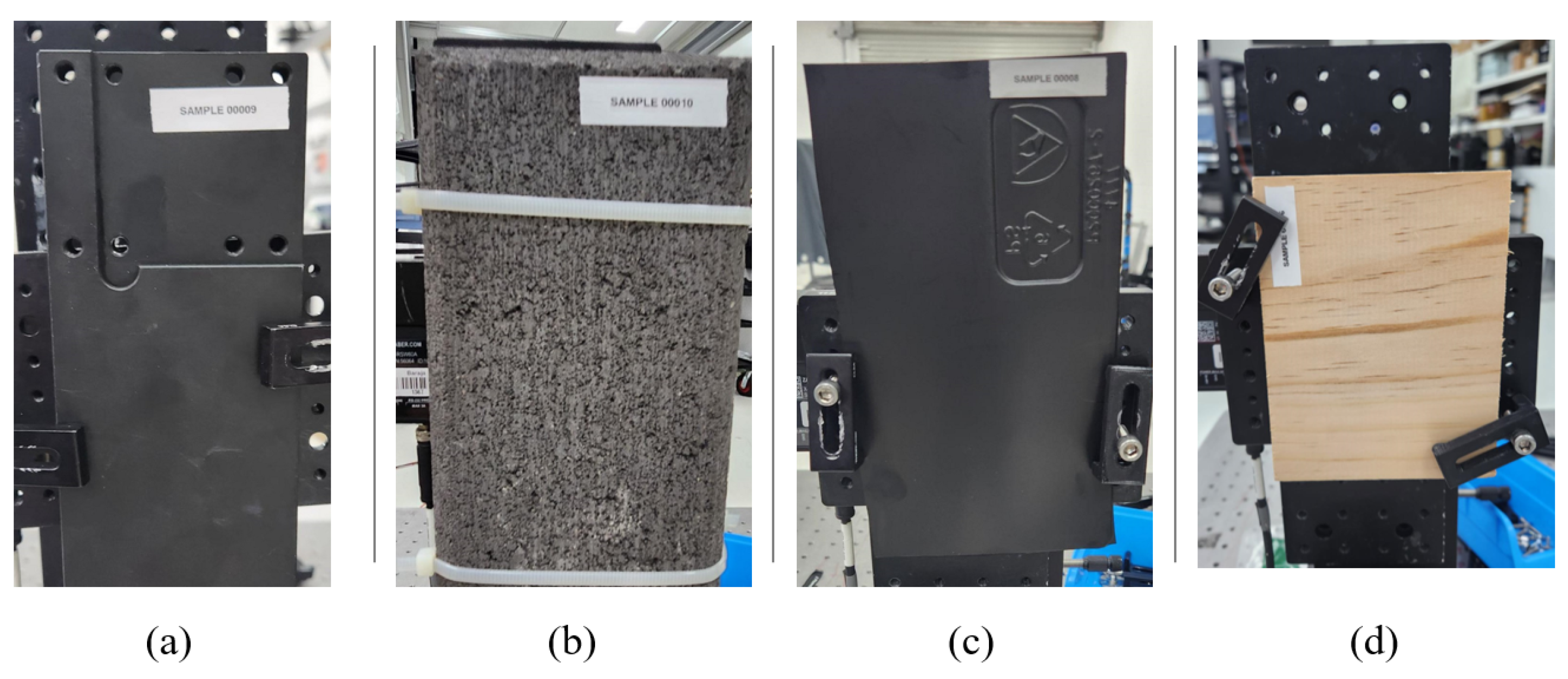
The set of materials used in our experiment are four that would occur in an urban environment: black power-coated aluminum, concrete, engineered wood and black plastic; photos of the samples are shown in Figure 5. The samples are large enough for our laser beam to entirely fit without clipping. In order to assess the classification performance of the polarization-diverse RMCW LIDAR, we sought to collect data in controlled experimental conditions, but with predetermined variations that would mimic a situation in a real environment. To this end, we collected data for every material sample and varying the target distance, the angle of incidence to the LIDAR (which we call yaw), the rotation of the material in the plane perpendicular to the LIDAR optical path (which we call roll), and the polarization of the transmit signal from the RMCW LIDAR. These deliberate variations are to explore the range of polarizations that we receive in the BOSA, and to validate the classifier with these variations.
The variations are explored using a full-factorial design-of-experiments (DOE), and the values used in the input factors is shown in Table 1. For each one of the 108 combinations, we collect roughly 830 measurements for a total of more than 89 640 measurements per material; using our RMCW reference code, we correlate the return signal and use a constant false alarm rate (CFAR) algorithm to determine if we have a valid peak, using a false alarm rate of 1e-4 [28]. If no peaks are passed through CFAR, we reject the measurement completely.

5. Results

As described in Section 4.1, each material was tested according to the DOE plan, with the polarization-diverse quadrature signals digitized and recorded for every configuration for each material. Thus, we store more than 89 000 measurements for each material, and each measurement is processed to produce a distance to target, the SNR of the cross-correlation peak, and the four Stokes parameters. Therefore, in total, we collected 356 000 measurements to train and validate our classifier, with the DOE ensuring we have significant real-world variation in the dataset.
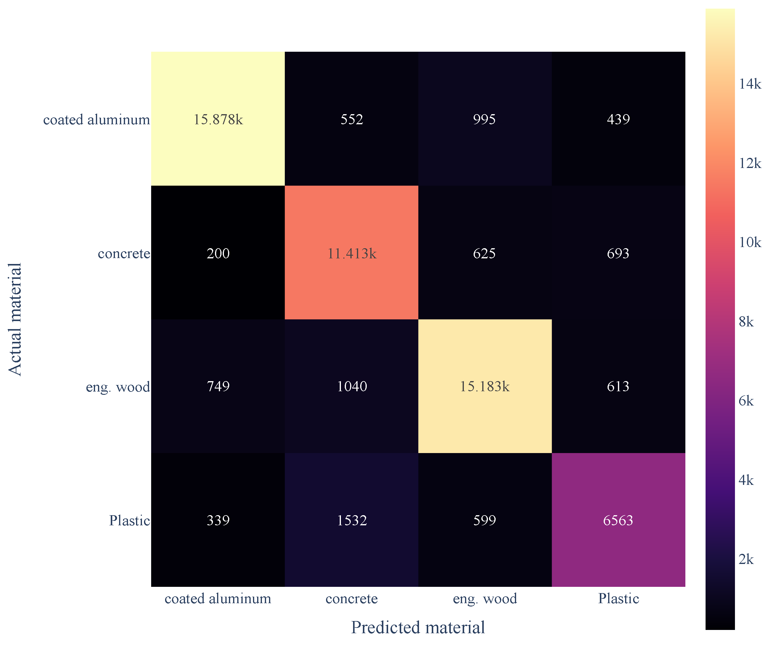
These six measurement outputs are the six inputs to our neural network, We then trained a single hidden layer neural network, with 64 nodes, as described in Section 2.3, and then run the resulting model on the validation data set. We express the performance of the classifier with a confusion matrix, as shown in Figure 6. The overall classification accuracy is 85.4%; however, from the confusion matrix it is clear that the majority of the misclassifications come from plastic, which has a classification accuracy of just 72.6%.
To explore the performance of the classifier with the hidden node number of neurons, we repeated the training and validation for a selection of hidden layer sizes, and measured the overall classification accuracy, shown in Figure 8.
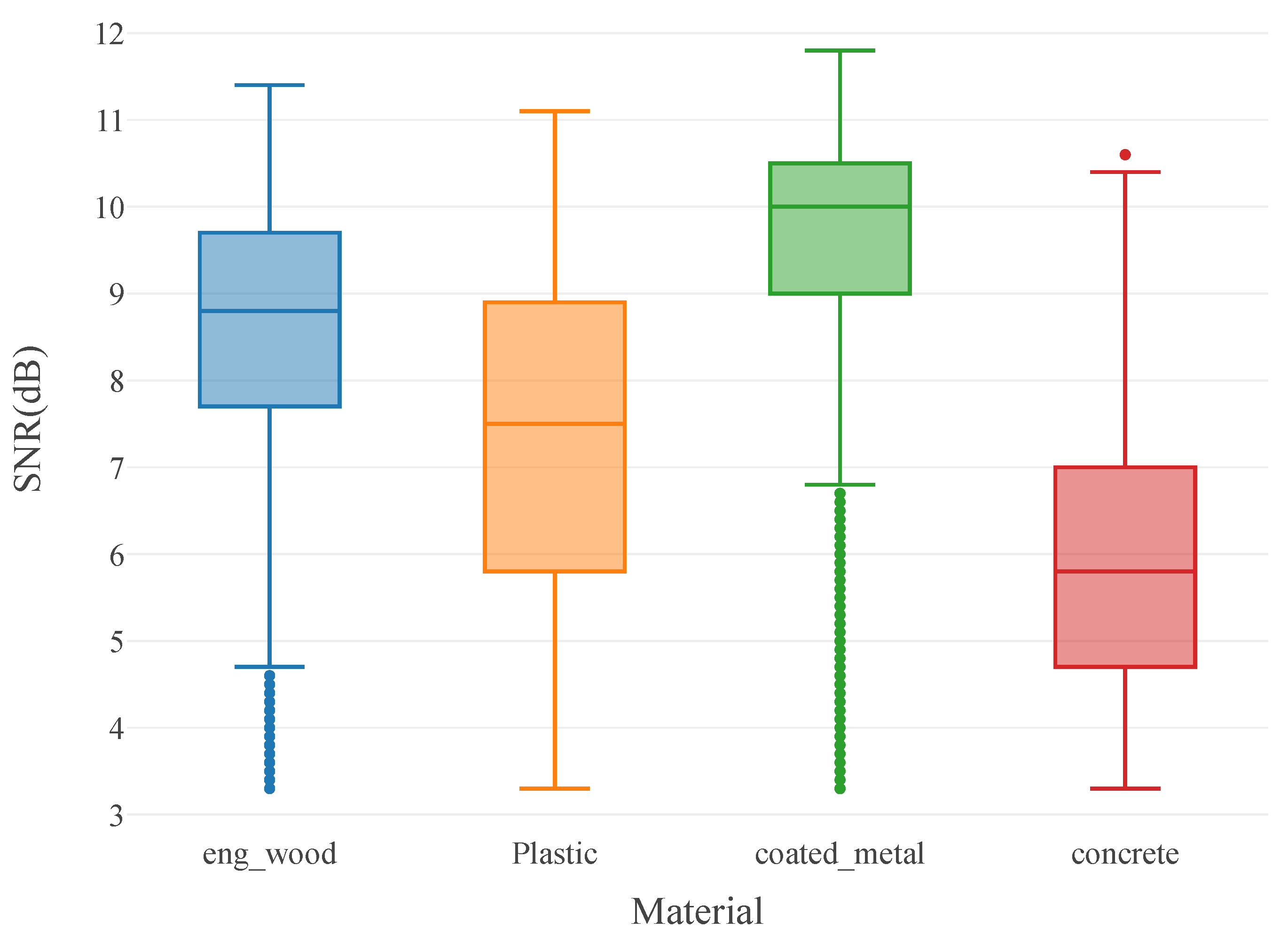
Figure 7. Distribution of SNR values for all materials in dataset.
Preprints 100988 g007
Figure 8. Classification accuracy as number of nodes in hidden layer increase.
Preprints 100988 g008
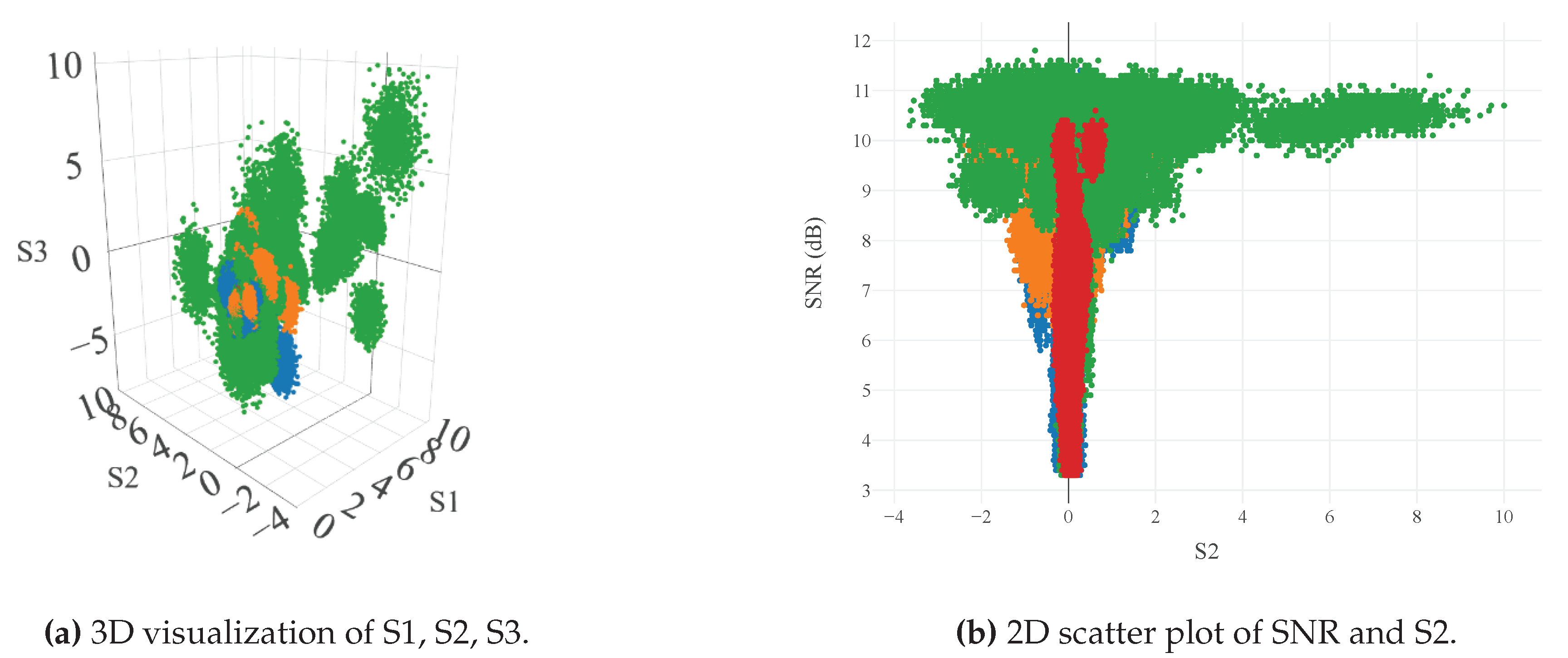
We use a 3D scatter plot to visualize the Stokes parameters, S1, S2, S3, and understand if the measurements demonstrate that the materials show differing polarization results; note that we remind the reader that the launch conditions were 0°, 45°, and 90°linear polarization relative to the output window of the LIDAR sensor. As shown in Figure 9a, all materials have measured Stokes parameters that are well clustered; the exceptions are concrete (in purple), which is clustered, but not visible, and coated metal, which is clustered into many smaller groupings. This would suggest that classification on concrete would have poor accuracy, and that most of the false classifications would be for coated aluminum. In contrast, the confusion matrix in Figure 6 indicates a different conclusion; the accuracy for concrete is 88.3%, and the false reading is highest for plastic.
Additional insight is available by plotting the relationship between SNR and the Stokes parameters; in Figure 9b, we see a clear distinction between concrete and the other materials, as concrete is strongly confined in S2 but greatly dispersed in SNR. Similarly, we note that coated metal only has measurement points above SNR > 8 dB.
6. Conclusion

We have demonstrated instantaneous material classification using an RMCW LIDAR system with an integrated transmit/receive photonic chip to enable polarization-diverse homodyne detection. This technique enables the creation of LIDAR point clouds with a point-by-point estimate of materials in the environment, which could greatly aid perception tasks for autonomous vehicles and robotics. In our field test at 3m and 10m, we varied angle of incidence and rotation normal to the LIDAR, as well as the launch polarization state, collecting over 350 000 measurements to train and validate our machine learning model for material classification. The field test demonstrated that plastic, engineered wood, concrete and coated aluminum could be correctly classified with an accuracy of 85.4%. We believe that this is a strong demonstration of material classification as a novel LIDAR data product for autonomy and robotics.

Author Contributions

Conceptualization, C.P., Y.K. and F.C.; methodology, Y.K.; software, C.P.; experimental validation, D.R.; writing—original draft preparation, C.P. and A.T.; writing—review, Y.K. and F.C.

Acknowledgments

The authors would like to acknowledge the contributions of Ben Hopkins, who assisted with the details on polarization and the optical system.

Conflicts of Interest

The authors disclose that they are full-time employees of Baraja Pty Ltd. and/or Baraja Inc., where they are actively commercializing LIDAR technology.

References

  1. Hecht, J. Lidar for self-driving cars. Optics and Photonics News 2018, 29, 26–33. [Google Scholar] [CrossRef]
  2. Fernando, H.; Marshall, J. What lies beneath: Material classification for autonomous excavators using proprioceptive force sensing and machine learning. Automation in Construction 2020, 119, 103374. [Google Scholar] [CrossRef]
  3. Kiyokawa, T.; Takamatsu, J.; Koyanaka, S. Challenges for future robotic sorters of mixed industrial waste: a survey. IEEE Transactions on Automation Science and Engineering 2022. [Google Scholar] [CrossRef]
  4. Tao, J.; Liang, R.; Li, J.; Yan, B.; Chen, G.; Cheng, Z.; Li, W.; Lin, F.; Hou, L. Fast characterization of biomass and waste by infrared spectra and machine learning models. Journal of hazardous materials 2020, 387, 121723. [Google Scholar] [CrossRef] [PubMed]
  5. Dashpute, A.; Saragadam, V.; Alexander, E.; Willomitzer, F.; Katsaggelos, A.; Veeraraghavan, A.; Cossairt, O. Thermal Spread Functions (TSF): Physics-guided Material Classification. Proceedings of the IEEE/CVF Conference on Computer Vision and Pattern Recognition, 2023, pp. 1641–1650.
  6. Shanbhag, H.; Madani, S.; Isanaka, A.; Nair, D.; Gupta, S.; Hassanieh, H. Contactless Material Identification with Millimeter Wave Vibrometry. Proceedings of the 21st Annual International Conference on Mobile Systems, Applications and Services, 2023, pp. 475–488.
  7. Tanaka, K.; Mukaigawa, Y.; Funatomi, T.; Kubo, H.; Matsushita, Y.; Yagi, Y. Material classification from time-of-flight distortions. IEEE transactions on pattern analysis and machine intelligence 2018, 41, 2906–2918. [Google Scholar] [CrossRef] [PubMed]
  8. Muckenhuber, S.; Holzer, H.; Bockaj, Z. Automotive lidar modelling approach based on material properties and lidar capabilities. Sensors 2020, 20, 3309. [Google Scholar] [CrossRef] [PubMed]
  9. Kirchner, N.; Taha, T.; Liu, D.; Paul, G. Simultaneous material type classification and mapping data acquisition using a laser range finder. International Conference on Intelligent Technologies. University of Technology, Sydney, 2007.
  10. Antonarakis, A.; Richards, K.S.; Brasington, J. Object-based land cover classification using airborne LiDAR. Remote Sensing of environment 2008, 112, 2988–2998. [Google Scholar] [CrossRef]
  11. Lee, S.; Lee, D.; Kim, H.C.; Lee, S. Material Type Recognition of Indoor Scenes via Surface Reflectance Estimation. IEEE Access 2021, 10, 134–143. [Google Scholar] [CrossRef]
  12. Bonifazi, G.; Capobianco, G.; Palmieri, R.; Serranti, S. Hyperspectral imaging applied to the waste recycling sector. Spectrosc. Eur 2019, 31, 8–11. [Google Scholar] [CrossRef]
  13. Peyghambari, S.; Zhang, Y. Hyperspectral remote sensing in lithological mapping, mineral exploration, and environmental geology: an updated review. Journal of Applied Remote Sensing 2021, 15, 031501. [Google Scholar] [CrossRef]
  14. Liu, X.; Zhang, L.; Zhai, X.; Li, L.; Zhou, Q.; Chen, X.; Li, X. Polarization Lidar: Principles and Applications. Photonics. MDPI, 2023, Vol. 10, p. 1118.
  15. Sassen, K.; Zhu, J.; Webley, P.; Dean, K.; Cobb, P. Volcanic ash plume identification using polarization lidar: Augustine eruption, Alaska. Geophysical research letters 2007, 34. [Google Scholar] [CrossRef]
  16. Brown, J.P.; Roberts, R.G.; Card, D.C.; Saludez, C.L.; Keyser, C.K. Hybrid passive polarimetric imager and lidar combination for material classification. Optical Engineering 2020, 59, 073106–073106. [Google Scholar] [CrossRef]
  17. Nunes-Pereira, E.; Peixoto, H.; Teixeira, J.; Santos, J. Polarization-coded material classification in automotive LIDAR aiming at safer autonomous driving implementations. Applied Optics 2020, 59, 2530–2540. [Google Scholar] [CrossRef] [PubMed]
  18. Takeuchi, N.; Sugimoto, N.; Baba, H.; Sakurai, K. Random modulation cw lidar. Applied optics 1983, 22, 1382–1386. [Google Scholar] [CrossRef] [PubMed]
  19. Roudas, I.; Vgenis, A.; Petrou, C.S.; Toumpakaris, D.; Hurley, J.; Sauer, M.; Downie, J.; Mauro, Y.; Raghavan, S. Optimal polarization demultiplexing for coherent optical communications systems. Journal of Lightwave Technology 2010, 28, 1121–1134. [Google Scholar] [CrossRef]
  20. Pulikkaseril, C. Simulating correlation waveforms of random modulated continuous wave LIDAR. Optical Engineering 2022, 62, 031205. [Google Scholar] [CrossRef]
  21. echt, E. Optics; Pearson Education, Incorporated, 2017.
  22. JMP Statistical Discovery LLC. Neural Networks. Available online: https://www.jmp.com/support/help/en/17.2/index.shtml#page/jmp/neural-networks.shtml#103373 (accessed on 18 January 2024).
  23. Castaño, F.; Beruvides, G.; Haber, R.E.; Artuñedo, A. Obstacle recognition based on machine learning for on-chip LiDAR sensors in a cyber-physical system. Sensors 2017, 17, 2109. [Google Scholar] [CrossRef] [PubMed]
  24. Han, Y.; Salido-Monzú, D.; Butt, J.A.; Wieser, A. Polarimetric femtosecond-laser LiDAR for multispectral material probing. Optics and Photonics for Advanced Dimensional Metrology II. SPIE, 2022, Vol. 12137, pp. 70–77.
  25. Puttnam, B.J.; Luís, R.S.; Delgado Mendinueta, J.M.; Sakaguchi, J.; Klaus, W.; Kamio, Y.; Nakamura, M.; Wada, N.; Awaji, Y.; Kanno, A.; others. Self-homodyne detection in optical communication systems. Photonics. MDPI, 2014, Vol. 1, pp. 110–130.
  26. Fujii, Y. High-isolation polarization-independent optical circulator. Journal of Lightwave Technology 1991, 9, 1238–1243. [Google Scholar] [CrossRef]
  27. Matsumoto, T.; Sato, K.i. Polarization-independent optical circulator: an experiment. Applied Optics 1980, 19, 108–112. [Google Scholar] [CrossRef] [PubMed]
  28. Wikipedia contributors. Constant false alarm rate—Wikipedia, The Free Encyclopedia. 2022. Available online: https://en.wikipedia.org/w/index.php?title=Constant_false_alarm_rate&oldid=1104952768 (accessed on 18 January 2024).
Figure 1. (a) Example of a received RMCW signal corrupted by white noise, and (b) the resulting correlation signal showing a peak at the delayed time of the received waveform.
Preprints 100988 g001
Figure 2. a) MZM transfer function, operating point shown in red denotes the desired bias point to operate in phase-modulation. b) Input electrical modulation in the form of high and low voltages. c) Output optical modulation in the form of intensity and phase information. d) The transmit (TX) portion of the BOSA receives its input light from an external TOSA, which is then distributed between the Mach-Zehnder Modulator (MZM) and the path leading to the local oscillator.
Preprints 100988 g002
Figure 3. a) Single channel polarization-diverse IQ receiver. b) X/Y polarization constellation diagrams. Two example measurements are shown with their component breakdowns which are labelled on the receiver.)
Preprints 100988 g003
Figure 4. Experimental setup: we use a Tx BOSA for modulating RMCW code on the transmit path, and an RX BOSA for performing the polarization-diverse IQ demodulation, using unmodulated light as the local oscillator (DBR: distributed Bragg reflector, EDFA: erbium-doped fiber amplifier, PC: polarization controller, PBS: polarization beamsplitter).
Preprints 100988 g004
Figure 5. Materials used for experimental validation: (a) coated aluminum, (b) concrete, (c) black plastic, (d) engineered wood.
Preprints 100988 g005
Figure 6. Confusion matrix for 64-node classifier on four different materials.
Preprints 100988 g006
Figure 9. Scatter plots to demonstrate the clustering of measurements in polarization space, and with SNR. Points are colored by material, with concrete (red), coated metal (green), plastic (orange) and engineered wood (blue).
Preprints 100988 g009
Table 1. Experimental factors used in the full-factorial design-of-experiments (DOE) for collecting training and validation data.
Input factor Values
Distance (m) 3, 10
Tx polarization (°) 0, 45, 90
Yaw (°) 0, 7, 15
Roll (°) 0, 45, 135, 180, 225, 315
Disclaimer/Publisher’s Note: The statements, opinions and data contained in all publications are solely those of the individual author(s) and contributor(s) and not of MDPI and/or the editor(s). MDPI and/or the editor(s) disclaim responsibility for any injury to people or property resulting from any ideas, methods, instructions or products referred to in the content.
Copyright: This open access article is published under a Creative Commons CC BY 4.0 license, which permit the free download, distribution, and reuse, provided that the author and preprint are cited in any reuse.
Prerpints.org logo

Preprints.org is a free preprint server supported by MDPI in Basel, Switzerland.

Subscribe

© 2024 MDPI (Basel, Switzerland) unless otherwise stated