A Fault Diagnosis Method for CNC Machine Feed System Based on DoubleEnsemble-LightGBM Model

Preprint

Article

A Fault Diagnosis Method for CNC Machine Feed System Based on DoubleEnsemble-LightGBM Model

Altmetrics

Downloads

Views

Comments

A peer-reviewed article of this preprint also exists.

Yiming Li^*

,Yize Wang,Liuwei Lu,Lumeng Chen

Yiming Li^*

,Yize Wang,Liuwei Lu,Lumeng Chen

This version is not peer-reviewed

Submitted:

14 March 2024

Posted:

15 March 2024

You are already at the latest version

Alerts

Abstract

In order to solve the problem of fault diagnosis for CNC machine feed system under the condition of variable speed conditions, an intelligent fault diagnosis method based on multi-domain feature extraction and ensemble learning model is proposed. First, various monitoring signals including vibration signal, noise signal and current signal are collected. Then, the monitoring signals are preprocessed and the time-domain, frequency-domain and time-frequency domain feature indexes are extracted to construct a multi-dimensional mixed domain feature set. Finally, the feature set is putting into the constructed DoubleEnsemble-LightGBM model to realize the fault diagnosis of the feed system. The experimental results show that the model can achieve good diagnosis results under different working conditions for both the public data set and the feed system test bench data set, and the average overall accuracy is 91.07% and 98.06% respectively. Compared with XGBoost and other advanced ensemble learning models, the method has better accuracy. It provides technical support for the stable operation and intelligent of CNC machine tools..

Keywords:

Subject: Engineering - Mechanical Engineering

1. Introduction

According to statistics, among the failures of CNC, the mechanical body failure accounts for about 57%, and the electrical system failure accounts for about 37.5%.CNC system failure accounts for only 5.5%, and most of the current CNC machines have the self-diagnosis function of electrical and CNC systems [1]. Fault of mechanical body is the key and difficult point of current research. With the continuous development of data acquisition technology, information technology and artificial intelligence technology, Fault diagnosis methods have also experienced the development process from artificial experience diagnosis to intelligent diagnosis, from single sensor diagnosis to multi-sensor fusion diagnosis.

Grether [2] took Siemens CNC machines as the research object. According to the expert knowledge in the field of fault diagnosis, an ontology-based knowledge representation structure is proposed, and then the SimRank algorithm is used to calculate the similarity between the fault phenomenon and the fault cause in the case base to realize the fault diagnosis of the CNC machine. Wang [3] established the fault tree model of CNC machines, and on this basis, a deep neural network model is constructed to classify and identify the features. The average recognition rate of BP network after feature reduction is 86%. Kemal [4] used Morlet Wavelet analysis to extract the features of vibration signals of CNC machines, and then proposed a deep LSTM model for fault classification, which effectively improves the classification accuracy. Shan et al. [5] proposed to arrange multiple sensors at different positions of the ball screw. The fault location of the ball screw is realized by carrying out weight distribution on the fault sensitivity indexes of different sensors and combining with a convolutional neural network, Finally, the effectiveness of the method is verified by the ball screw test bench. Zhang et al. [6] applied a new unsupervised learning method, generalized normalized sparse filtering, to rolling bearing intelligence under complex working conditions. The experiment proves that the method can obtain higher diagnosis accuracy with less training samples. Chen et al. [7] proposed a multi-scale feature alignment CNN for bearing fault diagnosis under different working conditions. The displacement invariance of CNN is improved, and the effectiveness and advancement of the method are verified by rolling bearing experiments. Moslem [8] proposed a domain adaptive method based on deep learning for cross-domain ball screw fault diagnosis. A deep convolutional neural network is used for feature extraction, and the maximum average difference metric is proposed to measure and optimize the data distribution under different working conditions. The effectiveness of the proposed method is proved by the experiment with the monitoring data of the ball screw under real working conditions. Pandhare et al. [9] Collected the vibration acceleration signals at five different positions on the ball screw test bench. A data domain adaptive fault diagnosis method based on convolutional neural network is proposed. The method minimize that maximum average difference of the high-level representation between the source domain data and the target domain data. The average diagnostic accuracy of the model is 98.25%. Jin et al. [10] proposed an end-to-end adaptive anti-noise neural network framework without manual feature selection and denoising processing. The convolutional feature extraction part of the network takes the exponential linear unit as the activation function, the extracted features are learned and classified by a gated recurrent neural network improved by an attention mechanism, The accuracy of bearing fault diagnosis under the conditions of noise and variable load is effectively improved. Patel T H et al. [11] modeled the mixed fault, analyzed its vibration signal, and then recognized the mixed fault pattern. Abbasion S et al. [12] applied the combination of Wavelet packet decomposition and support vector machine to the mixed fault diagnosis of bearings. Lei Y G et al. [13] proposed a classification method based on adaptive fuzzy neural inference to diagnose the composite faults of electric locomotives. Delgado. M et al. [14] extracted fault features from the motor current signal and vibration signal, and used partial least squares to reduce the dimensionality of the extracted features and construct feature vectors. Finally, they used a support vector machine (SVM) model to achieve the diagnosis of motor interturn short-circuit fault; Yang et al. [15] first derived a prediction formula for motor faults, and then used a Kalman filter to track and estimate the change trend of motor speed to determine whether the motor has failed. Wang et al. [16] used a multi-task shared classifier based on incremental learning to achieve better fault diagnosis of support bearings under various working conditions. Li et al. [17] proposed a method based on attention mechanism to solve the problem of low accuracy and poor stability of the model caused by unbalanced data sets. Experiments show that the method has good diagnosis effect under unbalanced data conditions. Xu et al. [18] used an improved method of combining multi-scale convolutional neural network with feature attention mechanism to improve the generalization ability of the model. Zhang et al. [19] proposed an instance-based transfer learning method to solve the problem of insufficient labeled samples in the application of ball screw fault diagnosis. Azamfar et al. [20] proposed a deep adaptive fault diagnosis method for cross-domain fault diagnosis of ball screw. Wu et al. [21] adopted a fault diagnosis method combining domain antagonistic neural network and attention mechanism. Experimental results show that this method has great potential in cross-domain diagnosis of rolling bearings. Huang Min et al. [22] proposed a method to solve the problem of data distribution deviation in the fault diagnosis of support bearing migration. The experimental results show that the method can support bearing migration fault diagnosis suitable for different working conditions.

Based on the comprehensive analysis of the research status of fault diagnosis of feed system, this paper’s primary contributions can be summarized as follows:

In order to solve the problem of fault diagnosis of CNC machine feed system under variable speed conditions, a fault diagnosis method based on multi monitoring signals, multi domain feature extraction and DoubleEnsemble-LightGBM integrated learning model is proposed. The experimental results show that this method achieves better diagnosis effect than Xgboost and other advanced integrated learning models;
A variety of monitoring signals including vibration signal, noise signal and current signal are collected. The monitoring signals are preprocessed by singularity elimination, trend item elimination, Wavelet threshold denoising, and then the time-domain, frequency-domain feature indexes and IMF information entropy of the monitroring signals are extracted. Finally, the multi-dimensional mixed domain feature set is constructed;
Based on the LightGBM model, the DoubleEnsemble-LightGBM fault diagnosis model is constructed by introducing the sample reweighting mechanism based on learning trajectory and the feature selection mechanism based on shuffling technology, which realizes the intelligent fault diagnosis of CNC machine feed system.

2. Relevant Theories

2.1. CEEMDAN Decomposition and IMF Information Entropy

2.1.1. CEEMDAN Decomposition

CEEMDAN（Complete Ensemble Empirical Mode Decomposition with Adaptive Noise) overcomes the mode mixing problem of EMD by adding adaptive white noise. And can effectively reduce the residual white noise in the IMF components obtained after decomposition [23].

The specific process of CEEMDAN decomposition is as follows:

1. adding k times of random Gaussian white noise with mean value is 0 into the signal

x (t)

to be decomposed, construct the sequence

x_{i} (t)

of the k times experiment according to formula (1), where

i = 1, 2, \cdot \cdot \cdot, K

x_{i} (t) = x (t) + ε_{0} δ_{i} (t)

(1)

Where:

δ_{i} (t)

is the random Gaussian white noise added in the ith experiment;

ε_{0}

is the weight coefficient of the Gaussian white noise.

2. carry out EMD decomposition on that sequence

x_{i} (t)

, take the average value of the first IMF component obtained from the k times experiment as the first IMF component obtained from CEEMDAN decomposition, and see formula (2) for calculation. See formula (3) for the calculation of the residual signal after the first decomposition.

{\bar{I M F}}_{1} (t) = \frac{1}{K} \sum_{i = 1}^{K} I M F_{1}^{i} (t)

(2)

r_{1} (t) = x (t) - {\bar{I M F}}_{1} (t)

(3)

3. a new sequence

r_{1} (t) + ε_{1} E_{1} (δ_{i} (t))

is obtained by adding k times specific noise to

r_{1} (t)

, and the EMD decomposition is carried out, calculate the second IMF component obtained by CEEMDAN decomposition according to formula (4).

{\bar{I M F}}_{2} (t) = \frac{1}{K} \sum_{i = 1}^{K} E_{1} (r_{1} (t) + ε_{1} E_{1} (δ_{i} (t)))

(4)

Where:

E_{1} (\cdot)

is the first IMF component obtained after EMD decomposition;

ε_{1}

is the weight coefficient for adding noise to

r_{1} (t)

4. calculating a margin signal

r_{m} (t)

m = 2, \cdot \cdot \cdot, M

according to the formula (5), and obtaining the m+1th IMF component of the CEEMDAN in the same way as the step (3), See formula (6) for calculation.

r_{m} (t) = r_{m - 1} (t) - {\bar{I M F}}_{m} (t)

(5)

{\bar{I M F}}_{m + 1} (t) = \frac{1}{K} \sum_{i = 1}^{K} E_{1} (r_{m} (t) + ε_{m} E_{m} (δ_{i} (t)))

(6)

In the formula,

E_{m} (\cdot)

represents the mth IMF component obtained after EMD decomposition of a certain sequence;

ε_{m}

is the weight coefficient for adding noise to

r_{m} (t)

5. repeating the step (4) to calculate other IMF components of the CEEMDAN until the number of extreme points of

r_{m} (t)

is less than 2. Eventually, the signal

x (t)

is decomposed into m IMF components and a residual component

R (t)

R (t) = x (t) - \sum_{m = 1}^{M} {\bar{I M F}}_{m} (t)

(7)

2.1.2. False Modal Component Rejection

The IMF components obtained by CEEMDAN decomposition may contain false modal components, and the spurious modal components need to be rejected. The correlation coefficient can be used to describe the degree of correlation between the IMF component and the original signal. The closer the correlation coefficient is to 1, the more useful information the component contains, the stronger the correlation with the original signal is. Therefore, the false modal components after CEEMDAN decomposition can be adaptively eliminated through the correlation coefficient.

The correlation coefficient

C_{m}

between the mth IMF component and the original signal is calculated as follows:

C_{m} = \frac{\sum_{i = 1}^{N} (x_{i} - \bar{x}) (y_{i} - \bar{y})}{\sqrt{\sum_{i = 1}^{N} {(x_{i} - \bar{x})}^{2}} \sqrt{\sum_{i = 1}^{N} {(y_{i} - \bar{y})}^{2}}}

(8)

Where:

x_{i}

is the ith element value in the original signal sequence.

\bar{x}

is the average value of the original signal sequence.

y_{i}

is the value of the ith element in the mth IMF component.

\bar{y}

is the average value of the mth IMF component.

N

is the signal sequence length.

Albert et al. [24] gave a formula for calculating the adaptive threshold of the correlation coefficient, see Equation (9). If

C_{m} < μ

, then the mth IMF component will be rejected.

μ = \frac{\max (C_{m})}{10 \times \max (C_{m}) - 3}, m = 1, 2, \cdot \cdot \cdot, M

(9)

In the formula, M is the number of IMF components decomposed from the original signal and is

\max (C_{m})

the maximum correlation coefficient value.

2.1.3. Calculation of IMF Information Entropy

In the field of fault diagnosis, entropy can effectively reflect the complexity of the signal and describe its nonlinear characteristics. A single entropy value is often difficult to fully describe the signal characteristics, so extract multiple information entropy eigenvalues are extracted simultaneously. Assume that K effective IMF components are obtained after the signal

x (t)

is decomposed by CEEMDAN, denoted as

u_{i} (t), i = 1, 2, \cdot \cdot \cdot, k

1. Energy entropy of IMF

Energy entropy is an index that can characterize the energy complexity of a signal. The IMF energy entropy is calculated as follows:

First, the energy value of each effective IMF component is calculated by Equation (10):

E_{i} = \int_{- \infty}^{+ \infty} {| u_{i} (t) |}^{2} d t, i = 1, 2, \cdot \cdot \cdot, k

(10)

Then, the total energy value is calculated by Equation (11):

E = \sum_{i = 1}^{k} E_{i}

(11)

Finally, the IMF energy entropy is calculated by Equation (12):

H_{E} = - \sum_{i = 1}^{k} h_{i} \lg \begin{matrix} h_{i} \end{matrix}

(12)

Where:

h_{i} = E_{i} / E

represents the proportion of the energy value of the ith IMF component to the total energy value.

2. Power spectrum entropy of IMF

Power spectrum entropy can reflect the change of signal energy in frequency domain. The IMF power spectrum entropy is calculated as follows: First, each effective IMF component

u_{i} (t)

is Fourier transformed to obtain

u_{i} (ω), i = 1, 2, \cdot \cdot \cdot, k

. Then, the power spectrum of each effective IMF component is calculated by Equation (13):

S_{i} = \frac{1}{2 π N} {| u_{i} (ω) |}^{2}

(13)

Finally, the IMF power spectrum entropy is calculated by Equation (14):

H_{F} = - \sum_{i = 1}^{k} p_{i} \lg \begin{matrix} p_{i} \end{matrix}

(14)

Where:

p_{i} = S_{i} / \sum_{i = 1}^{k} S_{i}

represents the proportion of the power spectrum of the ith IMF component to the total power spectrum.

3. The singular spectral entropy of IMF

Singular spectral entropy can quantitatively describe the complex state characteristics of time series. The calculation of the IMF singular spectral entropy is as follows:

First, each IMF component is formed into a characteristic matrix A:

A = {[u_{1} (t), \cdot \cdot \cdot, u_{k} (t)]}^{T}

(15)

Then, the singular values

λ_{i}, i = 1, 2, \cdot \cdot \cdot, k

of the characteristic matrix A are computed.

Finally, the IMF singular spectral entropy is calculated by Equation (16):

H_{S} = - \sum_{i = 1}^{k} q_{i} \lg \begin{matrix} q_{i} \end{matrix}

(16)

Where:

q_{i} = λ_{i} / \sum_{i = 1}^{k} λ_{i}

represents the proportion of the ith singular value to the sum of all singular values.

2.2. LightGBM Algorithm

Light GBM [25] (Light Gradient Boosting Machine) is a lightweight gradient lifting model. It is an optimized implementation based on the classical ensemble learning model GBDT [26]. The principle of GBDT is shown in Figure 1.

The basic idea is to use the decision tree as a weak classifier, a plurality of weak classifiers are iteratively trained through a gradient lifting strategy, and all the weak classifiers are combined in a linear addition mode to form a strong classifier with better classification effect.

On the basis of GBDT, LightGBM is optimized as follows:

(1) Gradient-based One-Side Sampling (GOSS) algorithm is used to compress the training data samples without loss of accuracy, and its basic idea is to discard some samples that are not helpful to the calculation of information gain. Then the data calculation amount can be reduced, and the operation cost is greatly reduced.

(2) The Exclusive Feature Bundling (EFB) algorithm is used to merge the mutually exclusive features in high-dimensional data into one feature, which can effectively reduce the feature dimension and reduce the computational load.

(3) Histogram algorithm is used to improve the node segmentation strategy of decision tree. The basic idea is to discretize the continuous floating-point eigenvalues into K integers and construct a histogram with width K. This can greatly reduce the computational time and memory consumption, and has little impact on the overall classification accuracy of the model under the framework of gradient boosting. At the same time, it has the effect of regularization, which can prevent the model from overfitting and enhance the stability and robustness of the model.

(4) LightGBM uses a leaf-by-leaf growth strategy, which splits each time by finding the one with the largest split gain from all current leaf nodes, and so on. In the case of the same number of splits, the strategy of growing by leaves can reduce more errors and get better accuracy. However, in this way, a deeper decision tree may be grown, resulting in overfitting of the model, so the maximum depth limit is added to the growth strategy by leaf.

To sum up, LightGBM not only inherits the advantages of GBDT, but also greatly improves the training efficiency and memory consumption. Compared with other integrated learning models, this model is easier to deal with large-scale data, and requires low computing power of the equipment. Therefore, LightGBM is used as the basic model for mechanical fault diagnosis of feed system.

2.3. DoubleEnsemble Algorithm

Double Ensemble is a new ensemble algorithm framework that can be used with a variety of machine learning models. It includes two key technologies, one of which is the sample reweighting technology based on learning trajectory, which can give different weights to different samples in the process of model training, thus reducing the interference of simple samples and noise samples and enhancing the training of key samples. The feature selection technology based on shuffling mechanism can help the model to automatically screen sensitive features in the training process, thus effectively improving the accuracy of the model and reducing the risk of overfitting.

The algorithm flow (pseudocode) of DoubleEnsemble is shown in Table 1.

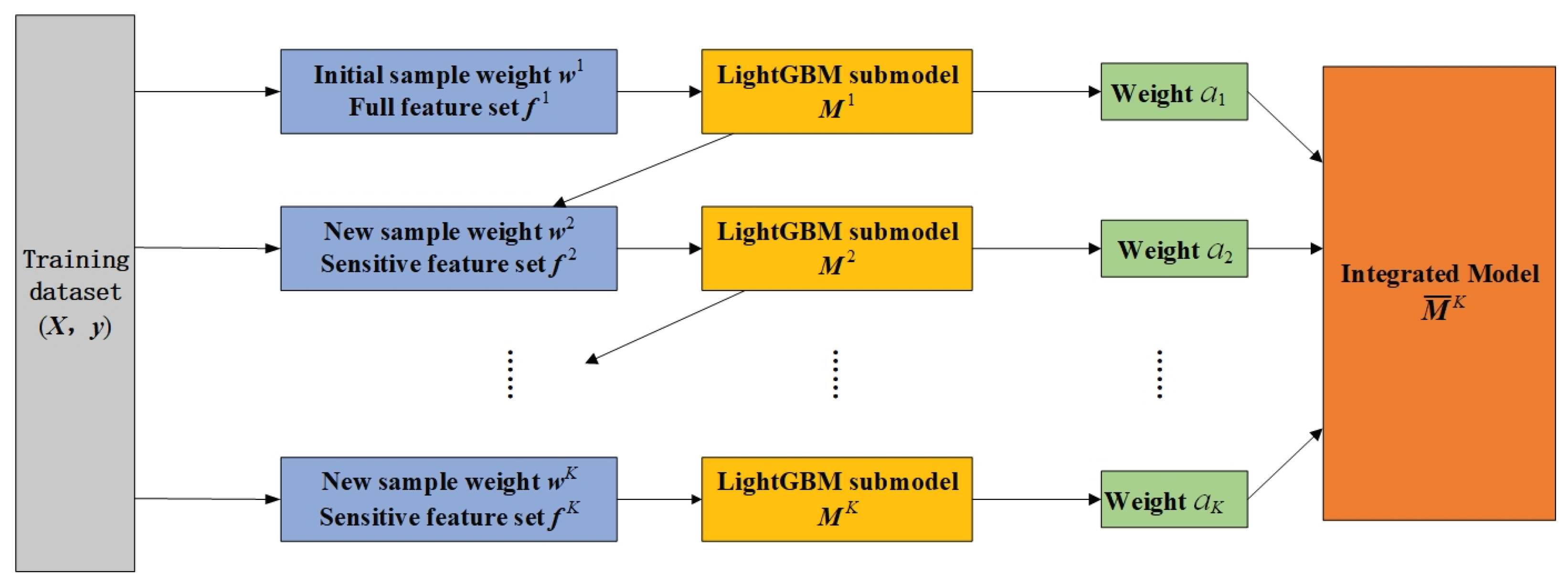
The algorithm sequentially trains K machine learning sub-models, denoted as

M^{1}

、···、

M^{K}

, all sub-models are weighted and integrated according to formula (17), and the integrated model

{\bar{M}}^{K} （ \cdot ）

is taken as the final output of the algorithm.

{\bar{M}}^{K} （ \cdot ） = \frac{1}{K} \sum_{i = 1}^{K} a_{i} M^{i} （ \cdot ）

(17)

Where:

a_{i}

is the weight coefficient of the ith sub-model

M^{i}

The training data consists of a feature matrix X and a label vector y.

X = {[x_{1}, \cdot \cdot \cdot, x_{N}]}^{T} \in R^{N \times F}

x_{i}

represents the feature set of the ith sample, N is the total number of training samples, and F is the dimension of the feature set.

y = (y_{1}, \cdot \cdot \cdot, y_{N})

y_{i}

represents the fault label of the ith sample. For the first sub-model

M^{1}

, the algorithm will use all the feature indexes in the feature set of the training data for training, i.e.,

f^{1}

= [F], the initial sample weights are set to

w^{1}

= (1,···,1). The subsequent sub-models are trained based on the newly selected feature set

f^{k} \subseteq [F]

and the updated sample weights

w^{k} = (w_{1}^{k}, \cdot \cdot \cdot, w_{N}^{k})

, Where

w^{k}

and

f^{k}

are obtained through sample re-weighting based on learning trajectory and feature selection based on shuffling mechanism algorithm [27], respectively.

3. Model: Multi-Domain Feature and DoubleEnsemble-LightGBM

The CNC machine feed system is a complex system with multi-mechanical components, and it is difficult to describe its fault state by the characteristics in a single domain. In order to reflect the health status of the feeding system more comprehensively, the time domain characteristic indexes, the frequency domain characteristic indexes and the time-frequency domain characteristic indexes of various monitoring signals including vibration signals, noise signals and current signals are firstly extracted, and a multi-dimensional mixed domain feature set as shown in Figure 2 is constructed.

In addition, considering that the total dimension of the multi-dimensional mixed domain feature set reaches hundreds of dimensions, it may contain invalid features, which will have a negative impact on model training.In addition, there may be simple samples and useless high noise samples in the collected training samples, which leads to poor training performance of the model and easy to overfit.Therefore, the fault diagnosis model is further optimized, and multiple LightGBM classification sub-models are trained and integrated through the DoubleEnsemble algorithm, so as to construct the DoubleEnsemble-LightGBM model as shown in Figure 3 for intelligent identification of the fault mode of the feed system.

4. Experimental Results

4.1. Data Set Description

4.1.1. University of Ottawa Variable Speed Bearing Failure Open Data Set

The vibration data of ER16K deep groove ball bearing under different speed conditions were collected from the variable speed bearing fault data set of the University of Ottawa in Canada, and the sampling frequency was 200 kHz. The fault types of bearings include: health, inner ring fault, outer ring fault, rolling element fault, and compound fault of inner and outer rings and rolling elements. Speed changes include: speed up (from 846 R/min to 1428 r/min), speed down (from 1734 r/min to 822 r/min), speed up first and then speed down (from 882 r/minute to 1518 r/minute and then to 1260 r/minutes), First decrease and then increase (from 1452 r/min to 888 r/min and then to 1236 r/min).

Firstly, five kinds of original data collected from the data set under four speed conditions (speed up, speed down, speed up and then speed down, speed down and then speed up) are divided into samples, and each sample contains 2000 data points. Then, the obtained samples are divided into the training set and the test set in a ratio of 8:2. The sample distribution of the data set and the corresponding relationship of the fault labels are shown in Table 2.

4.1.2. Dataset of Feed System Test Bench

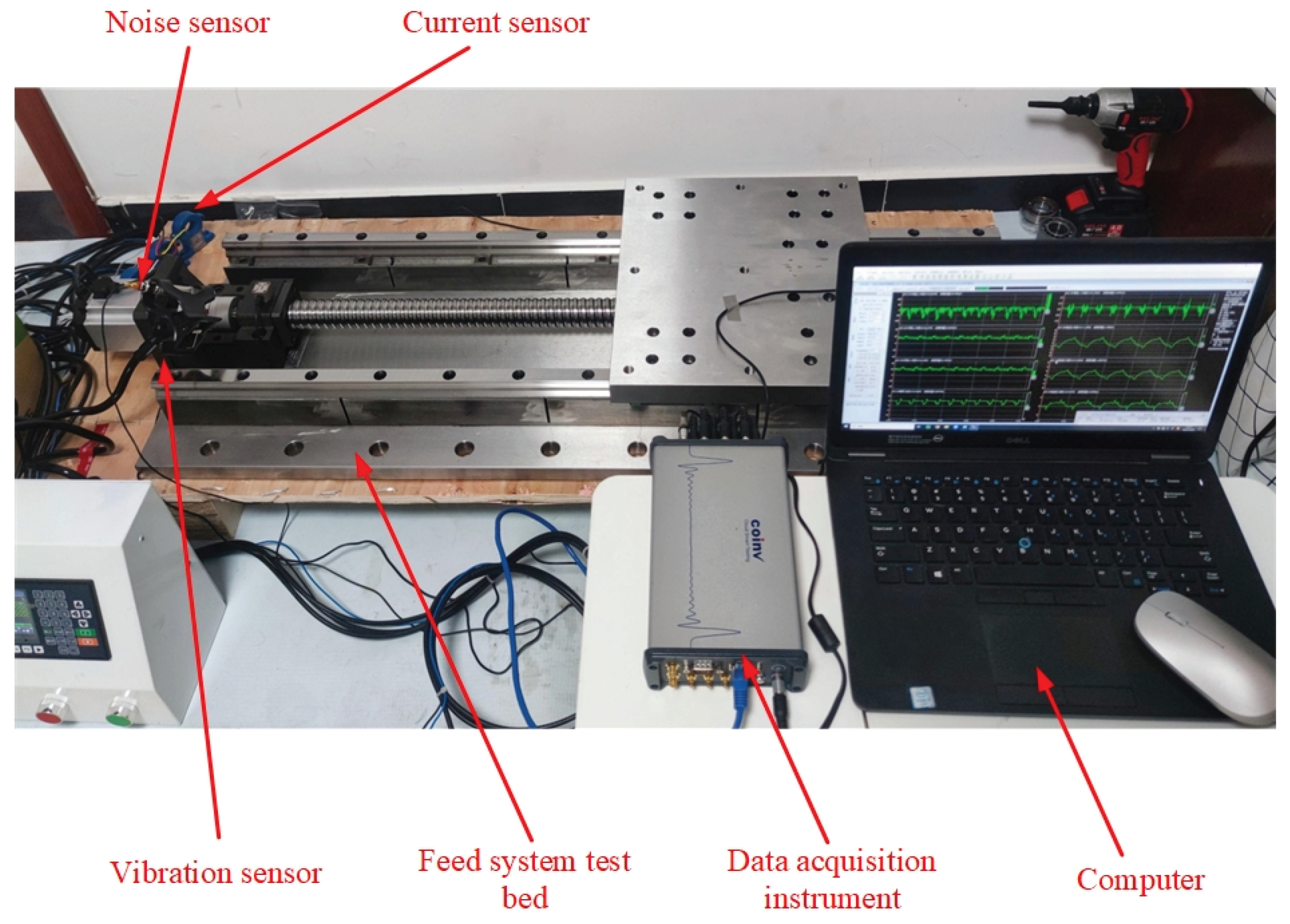
Based on the transmission principle and mechanical structure of the X-direction feed system of the vertical machining center, a feed system test bench as shown in Figure 4 is built.The test bench is made of heavy steel. The model and specification of the key parts used in the test are the same as those of the vertical machining center. The model of the ball screw pair is Taiwan Shangyin R4010FSI, the model of the rolling bearing is Japan NSK angular contact ball bearing 30TAC62B, the guide rail pair is a roller type rail with good rigidity, and the driving motor is a three-phase AC servo motor.

The model and parameters of the data acquisition equipment used in the experiment are shown in Table 3. Among them, the data acquisition instrument uses a high-precision distributed acquisition instrument developed by Beijing Dongfang Vibration Research Institute. The device has Ethernet and WIFI interfaces, supports multiple synchronous cascades, and can perform data acquisition through DASP software. The sensors used are three-directional vibration acceleration sensors, noise sensors produced by Beijing Dongfang Vibration Research Institute, and open-loop Hall current sensors produced by Beijing Senshe Electronics Co., Ltd.

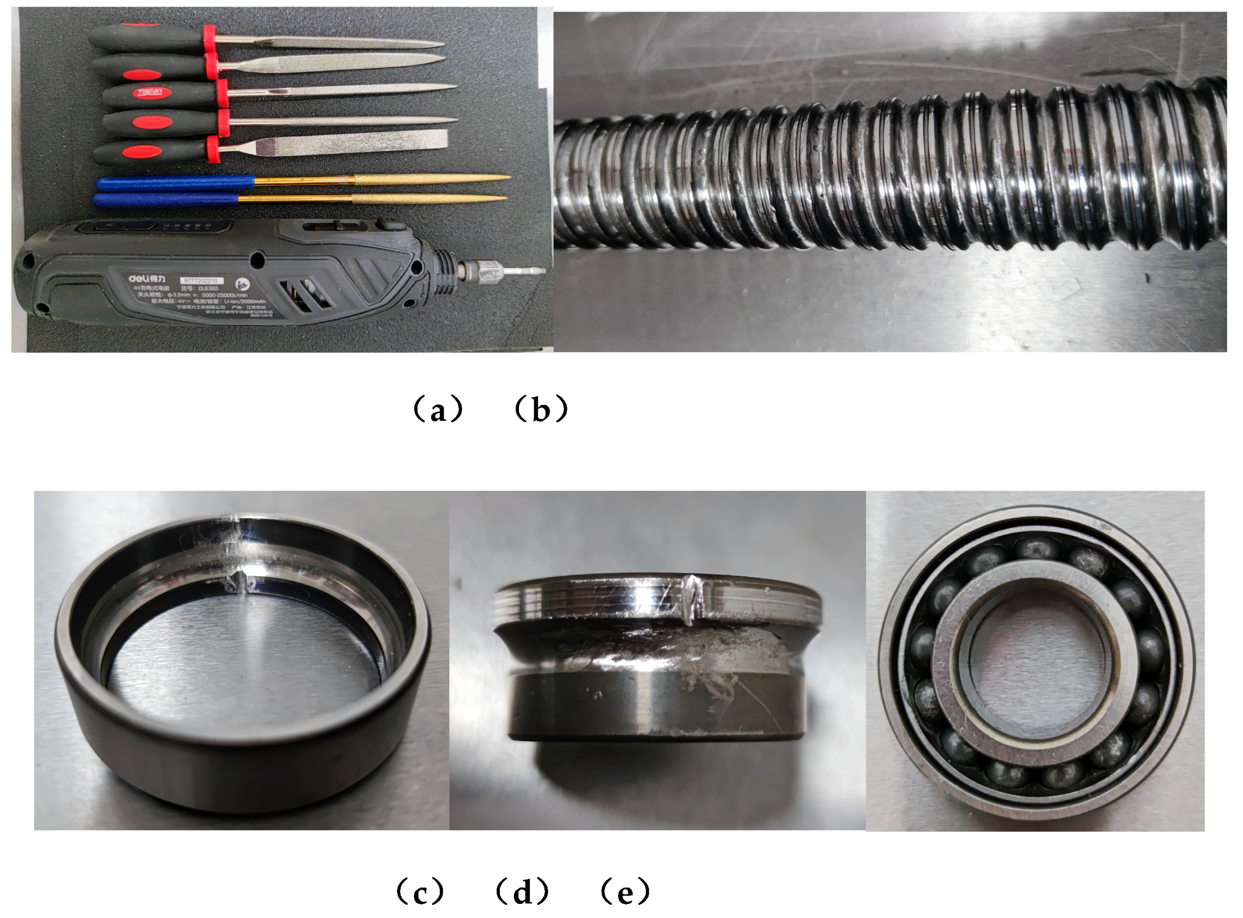
According to the historical fault statistics of feed system, the fault frequency of rolling bearing is the highest, accounting for 42% of all faults, and the fault frequency of ball screw pair is the second, accounting for 26% [28].Therefore, in order to collect the data of common fault types of rolling bearings and ball screw pairs, the tools such as file and electric grinding needle are used to make different degrees of wear or damage scars on the inner and outer rings of bearings and the raceways of screws, and the bearing balls are polished with sandpaper to make wear faults. Figure 5 shows the tools used and some of the manufactured fault parts.

In this experiment, the health data and fault data of three common feeding conditions were collected respectively. The feed rates of the cases 1 to 3 are set as 1000 mm/min, 2000 mm/min and 3000 mm/min, respectively. Fault types include: bearing inner ring fault, bearing outer ring fault, bearing ball fault, screw wear, screw bending, screw wear and bearing inner ring composite fault, screw wear and bearing outer ring composite fault, and screw wear and bearing ball composite fault. The collected signals include vibration signal, noise signal and current signal. The sampling frequency is 10 kHz, and the sampling time for each fault is 120 s. The fault data set divided by 2000 data points per sample is shown in Table 4.

4.2. Signal Preprocessing

(1) Elimination of singular point

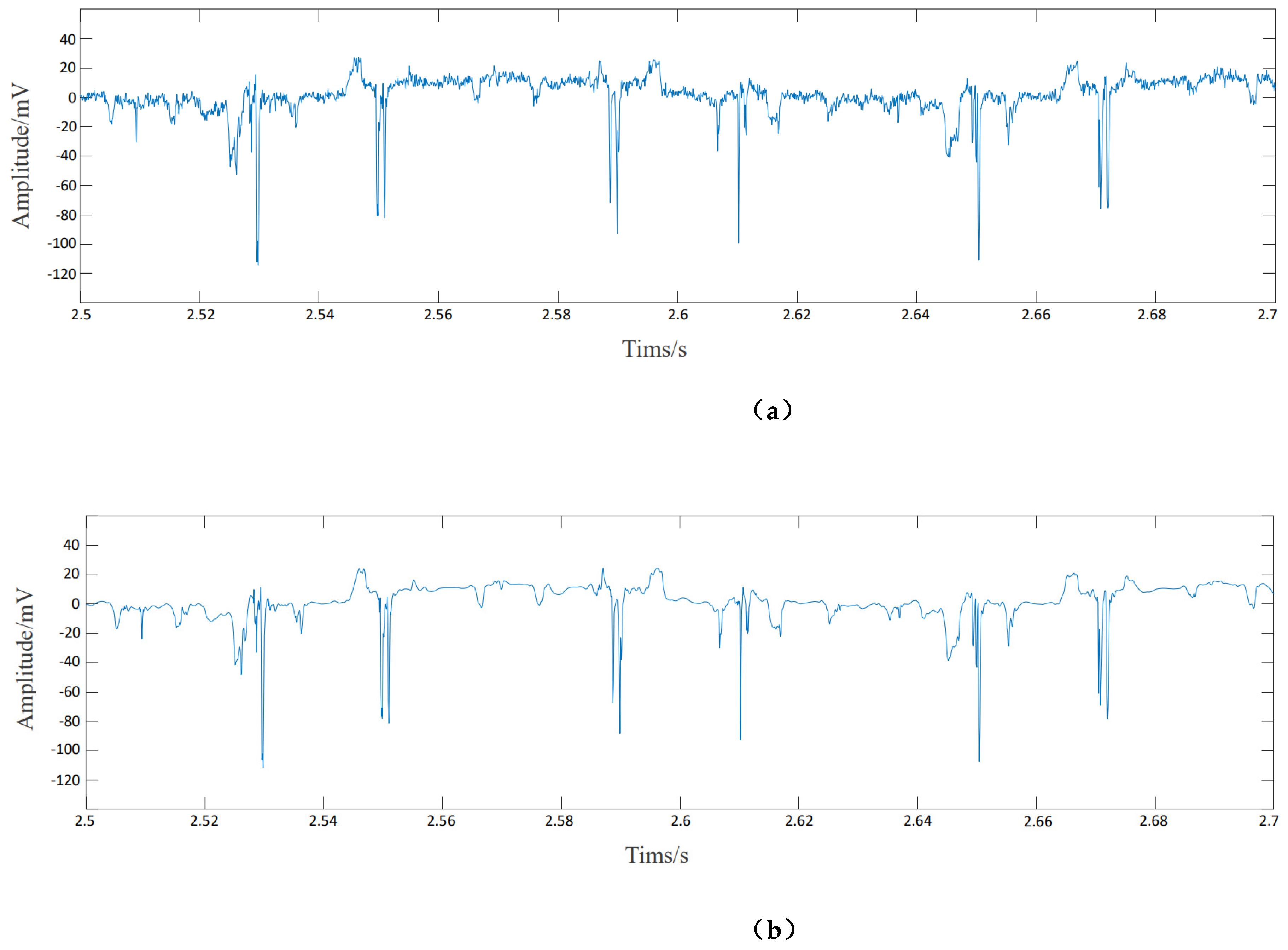
By setting the upper and lower threshold limits for the signal, the abnormal values outside the threshold range are eliminated. The empirical formula for the upper and lower limits of the threshold is the signal mean ± 4 signal standard deviations. Taking the noise sensor signal shown in Figure 6 (a) as an example, the calculated upper and lower threshold values are 5 and−5, respectively. The signal after removing the singular points is shown in Figure 6 (b).

(2) Elimination of trend term

In order to ensure the accuracy of the original data as much as possible, the signal trend line is fitted by the least square method and subtracted. Figure 7 (a) and (b) show the comparison of the X-direction vibration signals before and after the removal of the trend item.

(3) Wavelet threshold denoising

Wavelet threshold denoising is a nonlinear denoising method based on Wavelet transform. It is very suitable for processing non-stationary fault signals of CNC machines. In industrial signals, the fault signal mostly exists in the low-frequency component of the signal, while the noise is usually a high-frequency signal with a small amplitude [29]. The process of Wavelet threshold denoising is shown in Figure 8.

Sym5 is selected as the Wavelet base for signal denoising, and the original signal is decomposed by three-layer Wavelet. Then the soft and hard threshold compromise method is used for noise reduction, and the expression of the threshold function is shown as formula 18.

σ_{λ} (ω) = {\begin{matrix} sgn (ω) \cdot (| ω | - α λ), | ω | \geq λ \\ 0, | ω | < λ \end{matrix}

(18)

Where:

ω

is the Wavelet coefficient;

λ

is the threshold;

α

is the scaling factor, The value of

α

in this paper is 0.5.

Figure 9 shows the comparison between the original vibration signal and the signal after the above wavelet threshold denoising. It can be seen that this method effectively eliminates the high-frequency noise while retaining the main characteristic information of the original signal, and the denoising effect is good.

4.3. Signal Feature Extraction

(1) Time domain feature extraction

In order to reflect the overall situation of the signal and reflect the sudden change in the signal, 13 time domain characteristic indexes with dimension and non-dimension are extracted, as shown in Table 5. In the table,

{x_{i}}

is the discrete signal, and

i = 1, 2, \cdot \cdot \cdot, N

,N is the number of sampling points.

(2) feature extraction in frequency domain

Spectrum analysis can reflect the distribution and change of frequency components in the signal and provide effective fault information in the signal. The three extracted frequency domain characteristic indexes and their calculation are shown in Table 6.

(3) feature extraction in time-frequency domain

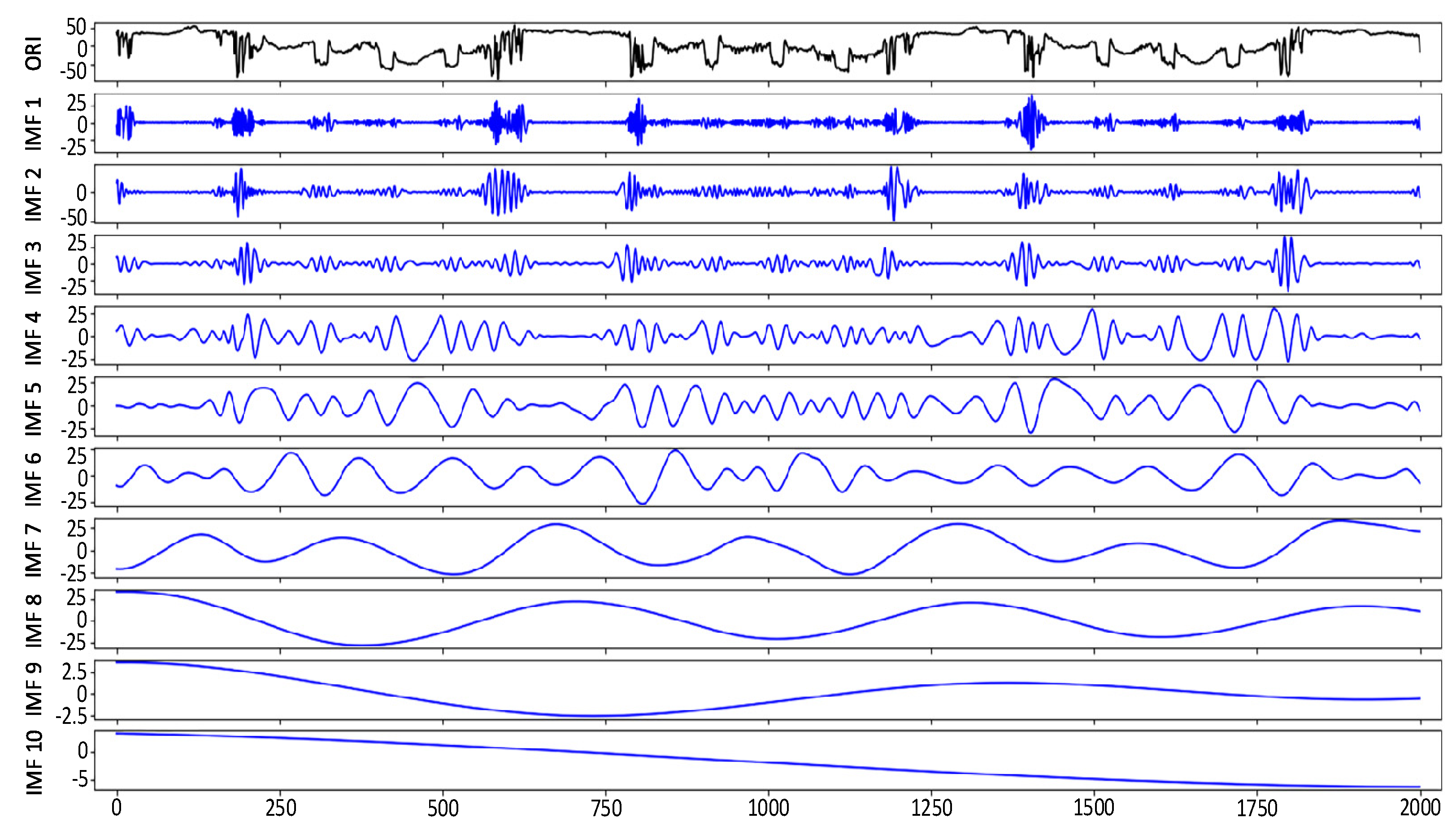
CEEMDAN is used to decompose the preprocessed signal to extract and select the effective IMF components, and then the information entropy of IMF components, such as energy, power spectrum and singular spectrum, is calculated. Taking the X-direction vibration signal of bearing ball wear fault as an example, the result of CEEMDAN decomposition is shown in Figure 10. The correlation coefficient between each IMF component and the original signal is shown in Table 7, and the correlation coefficient threshold can be calculated as 0.178 according to formula (9). Therefore, IMF 1, IMF 9 and IMF 10 will be removed, and IMF 2 ~ IMF8 will be retained as effective IMF components for subsequent signal feature extraction.

4.4. Experimental Environment, Hyper-Parameter Setting and Model Evaluation Index

(1) Experimental environment configuration

The experiment uses a self-configured server with Intel core i9 11900k CPU, 128GB running memory and 64-bit Windows 10 operating system. The development environment is LightGBM 3.2.1.99, Python 3.8.

(2) Hyperparameter setting

The training hyperparameters of the DoubleEnsemble-LightGBM fault diagnosis model are set as follows: the number of iterations (num_iterations) is 100,The learning_rate is 0.14, the maximum depth of the decision tree (Max _ depth) is 7, the number of leaf nodes (num _ leaves) is 21,The minimum sample number of leaf nodes (min_data _in_leaf) is 30, the number of sub-models is 5, and the weight of sub-models is (1,1,1,1,1).The number of sample subsets is 4, the feature sampling ratio is 80%, and the loss function is the classification cross entropy loss.

(3) Model evaluation index

Confusion matrix [30] is often used to judge the performance of multi-classification models. Table 8 shows the confusion matrix of the fault category prediction results. Where the number in the main diagonal position indicates the number of samples that the model correctly classifies for each fault, Larger indicates better model diagnostic performance. The numbers in the remaining positions represent the number of misclassified samples, and the smaller the number, the better the diagnostic performance of the model. Through the confusion matrix, it can be clearly distinguished which kind of fault is easy to be confused by the model.

The overall diagnosis accuracy and individual diagnosis accuracy are used as the evaluation indexes of the fault diagnosis model. The overall diagnostic accuracy can reflect the overall diagnostic performance of the model, as calculated in equation (19). The individual diagnostic accuracy can reflect the diagnostic performance of the model for a specific type of fault, as calculated in equation (20).

T = \frac{\sum_{i = 1}^{N} a_{i i}}{\sum_{i = 1}^{N} \sum_{j = 1}^{N} a_{j i}}

(19)

I_{i} = \frac{a_{i i}}{\sum_{j = 1}^{N} a_{j i}}, i = 1, 2, 3, \cdot \cdot \cdot N

(20)

Where:

T

is the overall diagnostic accuracy rate;

I_{i}

is the individual diagnostic accuracy rate;

a_{j i}

is the element value of the ith column of the jth row in the confusion matrix.

4.5. Analysis of Experimental Results

4.5.1. Analysis of Experimental Results of Public Data Set

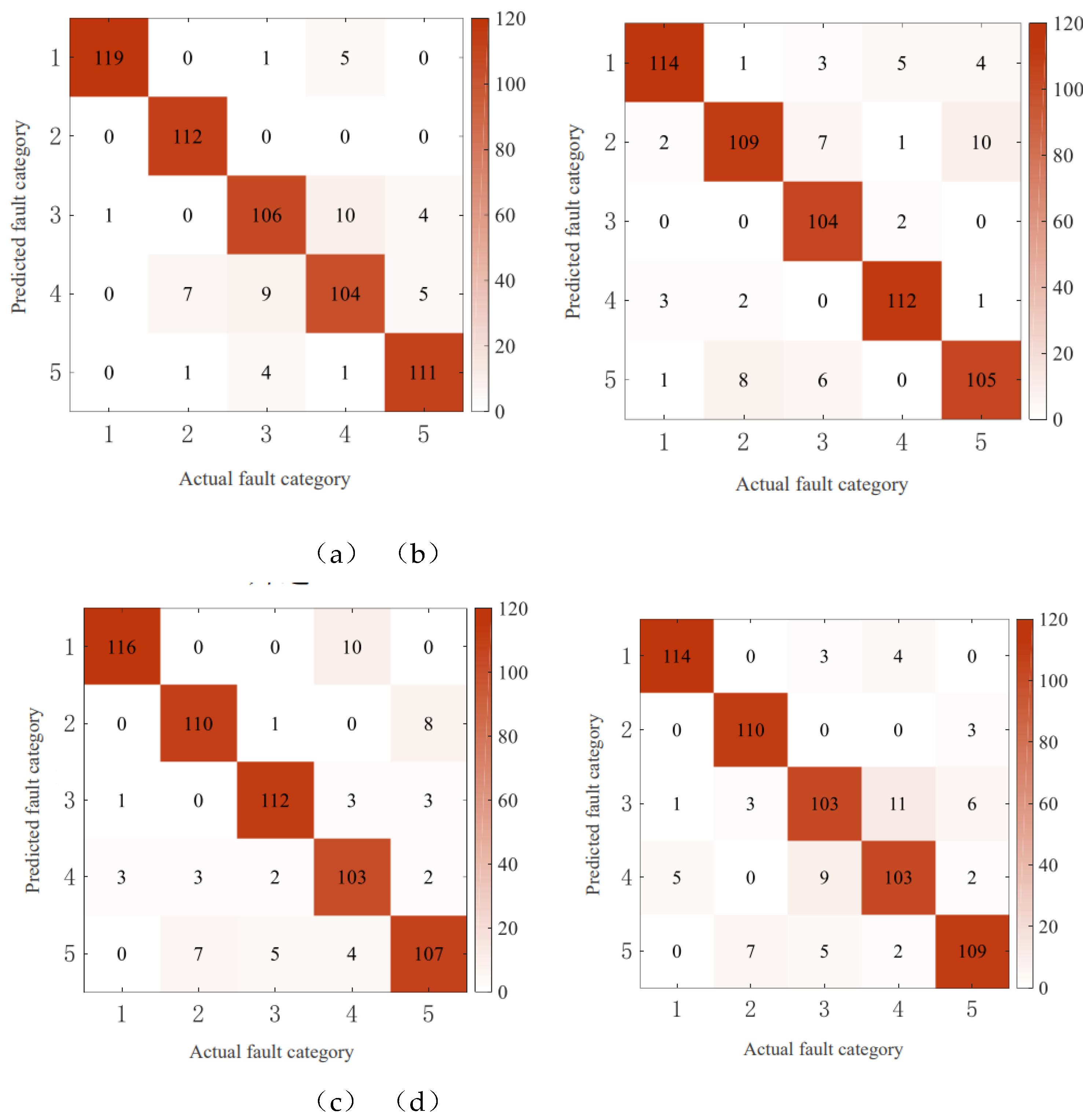
Considering the influence of random factors on model training and testing, 10 repeated experiments were carried out. Figure 11 shows the confusion matrix of the last experimental test result.

The overall diagnostic accuracy and individual diagnostic accuracy of the DoubleEnsemble-LightGBM model under each speed condition are calculated by analyzing the confusion matrix, and the calculation results are shown in Table 9.It can be seen from the table that the overall diagnostic accuracy of the model is 90.96% after averaging the calculation results under four speed conditions, which can achieve better overall diagnostic performance.The individual diagnostic accuracy of category 1 to category 5 is 96.46%, 91.88%, 88.54%, 87.92% and 90% respectively. It can be seen that the diagnostic accuracy of the model for category 1 (health) is the highest, and the diagnostic accuracy for category 3 (bearing ball failure) and category 4 (bearing outer ring failure) is lower.

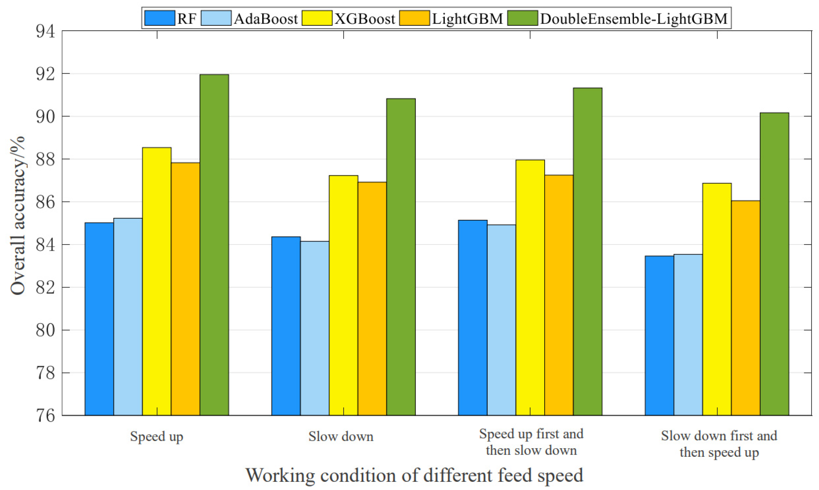
In addition, the diagnosis performance of the constructed DoubleEnsemble-LightGBM model is compared with that of the original LightGBM model and three other ensemble learning models with excellent performance in the field of fault diagnosis. The RF model used in [31], the AdaBoost model used in [32], and the XGBoost model in [33].The average value of the overall fault diagnosis accuracy of 10 experiments is taken as the evaluation index, and the experimental comparison results are shown in Table 10.It can be seen from the table that the average overall diagnostic accuracy of DoubleEnsemble-LightGBM model is the highest, which is increased by 6.57%, 6.61%, 3.42% and 4.06% respectively compared with RF model, AdaBoost model, XGBoost model and LightGBM original model. Figure 12 shows the comparison of the overall diagnostic accuracy of the five models under different speed conditions. The diagnostic performance of the Double Ensemble-Light GBM model is significantly better than that of other models.

4.5.2. Analysis of Experimental Results of Feed System Test Bench Data Set

Divide the feed system fault data set established by the feed system test bench in Section 4.1.2 into the training set and the test set at a ratio of 8:2. The distribution of the divided samples and the corresponding relationship of the fault labels are shown in Table 11.

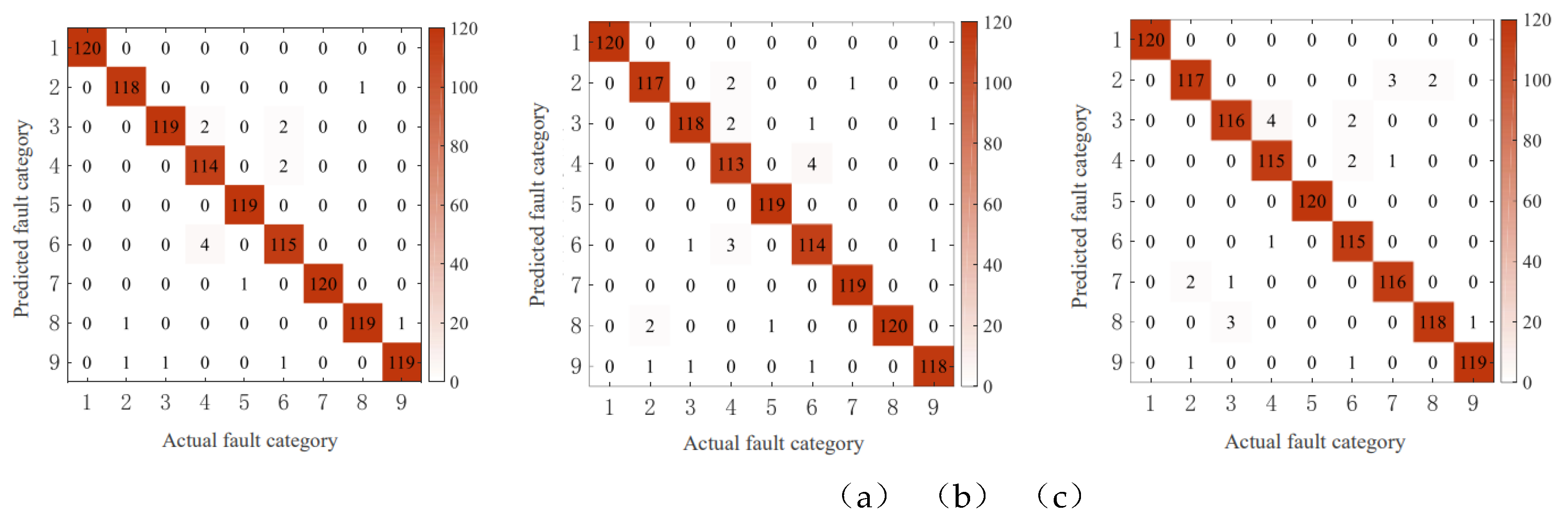
In order to ensure the reliability of the model, 10 repeated experiments were also carried out. Figure 13 shows the confusion matrix for the last experimental test result.

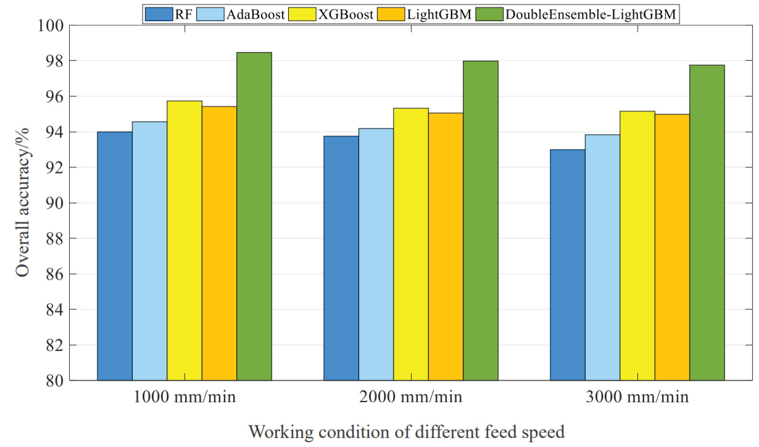
The overall diagnostic accuracy and individual diagnostic accuracy of the DoubleEnsemble-LightGBM model under each feed condition are calculated by analyzing the confusion matrix, and the calculation results are shown in Table 12.In the table, the feed speed corresponding to working condition 1, working condition 2 and working condition 3 is 1000 mm/min, 2000 mm/min and 3000 mm/min respectively. It can be seen from the table that after averaging the calculation results under the three feeding conditions, the overall diagnostic accuracy of the model is 98.06%, and the individual diagnostic accuracy of categories 1 to 9 is 100%, 97.78%, 98.06%, 95%, 99.45%, 95.55%, 98.61%, 99.17% and 98.89% respectively. The results show that the DoubleEnsemble-LightGBM model can achieve high-precision fault diagnosis, and the classification accuracy of health data (class 1) reaches 100%.

In addition, RF model, AdaBoost model, XGBoost model and LightGBM original model are also selected to compare the diagnostic performance with DoubleEnsemble-LightGBM model. The average value of the overall fault diagnosis accuracy of 10 experiments is taken as the evaluation index, and the experimental comparison results are shown in Table 13. It can be seen from the table that compared with the original LightGBM model, the average overall diagnostic accuracy of the constructed DoubleEnsemble-LightGBM model is improved by 2.91% under three feeding conditions, indicating that the introduction of sample reweighting and feature selection mechanism can effectively improve the overall diagnostic performance of the model. Compared with RF model, AdaBoost model and XGBoost model, the average overall diagnostic accuracy of DoubleEnsemble-LightGBM model is still the highest, which is improved by 4.48%, 3.87% and 2.66%, respectively. Figure 14 shows more intuitively the comparison of the overall diagnostic accuracy of the five models at different feed rates. The diagnostic performance of the Double Ensemble-Light GBM model is significantly better than that of the other models.

5. Conclusions and Future Work

In order to solve the problem of intelligent fault diagnosis of CNC machine feed system under variable speed conditions, a variety of signals such as current signal, vibration signal and noise signal are used as monitoring data. Firstly, the above signals are preprocessed by singularity elimination, trend item elimination, Wavelet threshold de-noising. Then, time-domain analysis and frequency-domain analysis are carried out for each signal, and 13 time-domain characteristic indexes and 3 frequency-domain characteristic indexes are extracted. The time-frequency analysis of the signal is carried out through CEEMDAN, and three IMF information entropy are calculated. The multi-dimensional mixed domain feature set is constructed by stitching the above multiple feature indexes into feature vectors. Finally, LightGBM is selected as the basic fault diagnosis model. In addition, in order to further improve the training performance of the model and improve the diagnosis accuracy, the sample reweighting mechanism based on learning trajectory and the feature selection mechanism based on shuffling technology are introduced to build a DoubleEnsemble-LightGBM fault diagnosis model. The experimental results show that the average diagnostic accuracy of the DoubleEnsemble-LightGBM model is 91.07% on the public variable speed bearing fault data set, and 98.06% on the self-built fault data set of the feed test bench. Compared with the RF, AdaBoost, Xgboost and other advanced ensemble learning models and the original LightGBM model, the proposed DoubleEnsemble-LightGBM model effectively improves the diagnostic accuracy on both data sets.

Due to the limitation of experimental conditions, the fault data of the key mechanical components of the feed system are mainly collected by building a feed test bench and artificially making simulated faults. The follow-up research will try to accumulate the real fault data of the actual work and production of the CNC machine feed system, and further expand the types of faults.

Author Contributions

The manuscript was heavily influenced by all of the contributors. Y.L. made important contributions to the study design, algorithm implementation, data management, chart production, and manuscript writing. L.C. provided project support for the study and made important contributions to the idea of the study, as well as the writing and review of the manuscript. Y.W. and L.L. made important contributions to the research literature search, data acquisition, and data analysis. All authors have read and agreed to the published version of the manuscript.

Funding

This research was funded by “High-Quality Development Project of the Ministry of Industry and Information Technology of the People’s Republic of China, Grant No. ZTZB-22-009-001”, “General Science and Technology Program of Beijing Municipal Education Commission Grant No. KM202011232011”and “Open project of Key Laboratory of modern measurement and control technology of Ministry of Education, Grant No. KF20221123205”.

Data Availability Statement

The dataset that are presented in this study can be obtained from https://data.mendeley.com/datasets/v43hmbwxpm/2

Conflicts of Interest

The authors declare no conflicts of interest.

References

Li Shan. Research on complex fault diagnosis of CNC machine tool feed system based on multi-source information fusion [D]. Qingdao University of Technology, 2016.
Michael, G.; Peng, J.; Marinov, M.B.; et al. Research on fault diagnosis expert system of cnc machine tool based on expert knowledge[C]//2021 International Scientific Conference Electronics (ET). IEEE, 2021: 1-4. IEEE,.
Wang, J. Error analysis and fault diagnosis of CNC machine tools under artificial intelligence technology[C]// Journal of Physics: Conference Series. IOP Publishing, 2021, 1881, 022085. [Google Scholar]
Polat, K. The fault diagnosis based on deep long short-term memory model from the vibration signals in the computer numerical control machines. Journal of the Institute of Electronics and Computer 2020, 2, 72–92. [Google Scholar] [CrossRef]
Shan, P.; Lv, H.; Yu, L.; et al. A multisensor data fusion method for ball screw fault diagnosis based on convolutional neural network with selected channels. IEEE Sensors Journal 2020, 20, 7896–7905. [Google Scholar] [CrossRef]
Zhang, Z.; Li, S.; Wang, J.; et al. General normalized sparse filtering: A novel unsupervised learning method for rotating machinery fault diagnosis. Mechanical Systems and Signal Processing 2019, 124, 596–612. [Google Scholar] [CrossRef]
Chen, J.; Huang, R.; Zhao, K.; et al. Multiscale convolutional neural network with feature alignment for bearing fault diagnosis. IEEE Transactions on Instrumentation and Measurement 2021, 70, 1–10. [Google Scholar] [CrossRef]
Azamfar, M.; Li, X.; Lee, J. Intelligent ball screw fault diagnosis using a deep domain adaptation methodology. Mechanism and Machine Theory 2020, 151, 103932. [Google Scholar] [CrossRef]
Pandhare, V.; Li, X.; Miller, M.; et al. Intelligent diagnostics for ball screw fault through indirect sensing using deep domain adaptation. IEEE Transactions on Instrumentation and Measurement 2020, 70, 1–11. [Google Scholar] [CrossRef]
Jin, G.; Zhu, T.; Akram, M.W.; et al. An adaptive anti-noise neural network for bearing fault diagnosis under noise and varying load conditions. IEEE Access 2020, 8, 74793–74807. [Google Scholar]
H, Darpe A K. Coupled bending-torsional vibration analysis of rotor with rub and crack. Journal of Sound and Vibration 2009, 326, 740–752. [Google Scholar] [CrossRef]
Abbasion, S.; Rafsanjani, A.; Farshidianfar, A.; et al. Rolling bearing element bearings mufti-fault classification based on the wavelet denoising and support vector machine. Mechanical Systems and Signal Processing 2007, 21, 2933–2945. [Google Scholar]
Lei Y G, He Z J, Zi Yanyang. Application of a novel hybrid intelligent method to compound fault diagnosis of locomotive roller bearings. ASME Transactions on Journal of Vibration and Acoustics 2008, 130, 1–6. [Google Scholar]
Delgado, M.; Garcia, A.; Ortega, J.A.; et al. Multidimensional intelligent diagnosis system based on support vector machine classifier[C]//2011 IEEE International Symposium on Industrial Electronics. IEEE, 2011: 2124-2131.
Yang, S. An experiment of state estimation for predictive maintenance using Kalman filter on a DC motor. Reliability engineering & system safety 2002, 75, 103–111. [Google Scholar]
Wang, P.; Xiong, H.; He, H. Bearing fault diagnosis under various conditions using an incremental learning-based multi-task shared classifier. Knowledge-Based Systems 2023, 266, 110395. [Google Scholar]
Li, J.; Liu, Y.; Li, Q. Intelligent fault diagnosis of rolling bearings under imbalanced data conditions using attention-based deep learning method. Measurement 2022, 189, 110500. [Google Scholar]
Xu, Z.; Li, C.; Yang, Y. Fault diagnosis of rolling bearings using an improved multi-scale convolutional neural network with feature attention mechanism. ISA Transactions 2021, 110, 379–393. [Google Scholar] [CrossRef]
Zhang, L.; Guo, L.; Gao, H.; et al. Instance-based ensemble deep transfer learning network: A new intelligent degradation recognition method and its application on ball screw. Mechanical Systems and Signal Processing 2020, 140, 106681. [Google Scholar]
Azamfar, M.; Li, X.; Lee, J. Intelligent ball screw fault diagnosis using a deep domain adaptation methodology. Mechanism and Machine Theory 2020, 151, 103932. [Google Scholar]
Wu, H.; Li, J.; Zhang, Q.; et al. Intelligent fault diagnosis of rolling bearings under varying operating conditions based on domain-adversarial neural network and attention mechanism. ISA Transactions 2022, 130, 477–489. [Google Scholar] [CrossRef]
Huang, M.; Yin, J.; Yan, S.; et al. A fault diagnosis method of bearings based on deep transfer learning. Simulation Modelling Practice and Theory 2023, 122, 102659. [Google Scholar] [CrossRef]
Shanshan, S.; Shuqing, Z.; Wei, D.; et al. A new hybrid method for bearing fault diagnosis based on CEEMDAN and ACPSO-BP neural network. Journal of Mechanical Science and Technology 2023, 37, 5597–5606. [Google Scholar]
Ayenu-Prah, A.; Attoh-Okine, N. A criterion for selecting relevant intrinsic mode functions in empirical mode decomposition. Advances in Adaptive Data Analysis 2010, 2, 1–24. [Google Scholar]
Ke, G.; Meng, Q.; Finley, T.; et al. LightGBM: A highly efficient gradient boosting decision tree[C]//Proceedings of the 31st International Conference on Neural Information Processing Systems, 2017: 3149-3157.
Wei, D.; Qing, C.; Yuzhan, D.; et al. Fault Diagnosis Method of Intelligent Substation Protection System Based on Gradient Boosting Decision Tree. Applied Sciences 2022, 12, 8989–8989. [Google Scholar]
Daying, Q.; Wei, F.; Gabriel, D.; et al. A Novel Double Ensemble Algorithm for the Classification of Multi-Class Imbalanced Hyperspectral Data. Remote Sensing 2022, 14, 3765–3765. [Google Scholar]
Zhu Jiwei. Health evaluation of feed system in machining center [D]. Jilin University, 2022.
Jared, N.; RR, H.; Andrew, G.; et al. Lightning forecast from chaotic and incomplete time series using wavelet de-noising and spatiotemporal kriging. Journal of Defense Analytics and Logistics 2023, 7, 90–102. [Google Scholar]
R,S. S S.Classification of yoga, meditation, combined yoga–meditation EEG signals using L-SVM, KNN, and MLP classifiers. Soft Computing 2024, 28, 4607–4619. [Google Scholar] [CrossRef]
Fei, C.; Liyao, Z.; Wenshen, L.; et al. A fault diagnosis method of rotating machinery based on improved multiscale attention entropy and random forests. Nonlinear Dynamics 2023, 112, 1191–1220. [Google Scholar]
Jiahui, J.; Yuqing, L.; Chaozheng, X.; et al. Research on Motor Bearing Fault Diagnosis Based on the AdaBoost Algorithm and the Ensemble Learning with Bayesian Optimization in the Industrial Internet of Things. Security and Communication Networks 2022, 2022. [Google Scholar]
Zhiguo, L.; Lijun, Z.; Xizhe, W. A Novel Intelligent Method for Fault Diagnosis of Steam Turbines Based on T-SNE and XGBoost. Algorithms 2023, 16, 98–98. [Google Scholar]

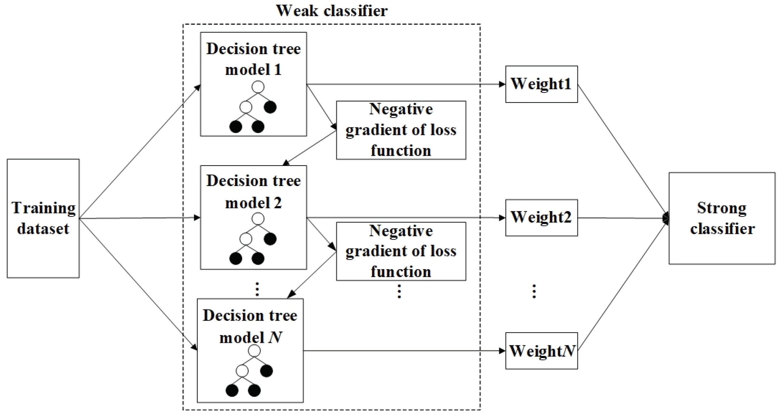
Figure 1. Principle of GBDT classification model.

Figure 2. Multi-dimensional mixed domain feature extraction.

Figure 3. Fault diagnosis model of DoubleEnsemble-LightGBM.

Figure 4. Feed System Test Bench.

Figure 5. Tools for preparation of defective parts and some defective parts. (a) Tool used; (b) Worn lead screw; (c) Bearing outer ring failure; (d) Bearing inner ring failure; (e) Bearing ball failure.

Figure 6. Comparison before and after singular point removal of noise signal. (a) Noise signal before singular point removal; (b) Noise signal after singular point removal.

Figure 7. Comparison of vibration signal before and after detrending. (a) Vibration signal before elimination of trend term; (b) Vibration signal after elimination of trend term.

Figure 8. Feed System Test Bench.

Figure 9. Comparison of original signal and denoised signal. (a) Original vibration signal; (b) Vibration signal after noise reduction.

Figure 10. CEEMDAN decomposition result of X-direction vibration signal.

Figure 11. Confusion matrix of the last experimental test result. (a) Speed up; (b) Speed down; (c) Up then down; (d) Down then up.

Figure 12. Comparison of diagnostic performance of different models under different speed conditions.

Figure 13. Confusion matrix of the last experimental test result. (a) Feed rate 1000 mm/min; (b) Feed rate 2000 mm/min; (c) Feed rate 3000 mm/min.

Figure 14. Comparison of diagnostic performance of different models under different feed conditions.

Table 1. Flow of DoubleEnsemble algorithm.

Algorithm: Double Ensemble

1: Input: Training data (X, y), number of sub-models K, and sub-model weights

a = (a_{1}, \cdot \cdot \cdot, a_{K})

2: Set the initial sample weights

w^{1}

= (1, ······, 1)

3: Select initial feature set

f^{1}

= [F]

4：for k=1 to K ：

M^{k}

← Train sub-model (X, y,

w^{k}

f^{k}

)

6: Retrieve the loss curve

C^{k}

of the sub-model

M^{k}

and the loss

L^{k}

of the current integrated model

{\bar{M}}^{k}

7: Update sample weights based on sample reweighting technique

w^{k + 1}

← SR (

C^{k}

L^{k}

,K)

8: Update feature set based on feature selection technique

f^{k + 1}

← FS (

{\bar{M}}^{k}

, X, y)

9: Return: Integrated model

{\bar{M}}^{K} （ \cdot ）

Table 2. Sample Distribution of Data Set and Corresponding Relationship of Fault Labels.

Label	Category	Number of training set samples	Number of test set samples
1	Health	480	120
2	Bearing inner ring failure	480	120
3	Bearing ball failure	480	120
4	Bearing outer ring failure	480	120
5	Bearing compound failure	480	120

Table 3. Model and Parameters of Data Acquisition Instrument and Sensor.

Device name	Equipment model	Device parameters
Data acquisition instrument	INV3062C	Sampling frequency range: 0.4~ 216 kHz; resolution: 24 bits; number of channels: 8
Three-direction vibration sensor	INV9832	Frequency range: 1-10 kHz; sensitivity: 100 mV/G;
Noise sensor	INV9206	Frequency range: 20 Hz ~ 20 kHz; sensitivity: 50 mV/Pa
Hall current sensor	CHK-100R1	Frequency range: from 0 to 20 kHz

Table 4. Self-built fault data set of feed system test bench.

Type of fault	Number of samples
Type of fault	Condition 1	Condition 2	Condition 3
Health	600	600	600
bearing inner ring fault	600	600	600
bearing outer ring fault	600	600	600
bearing ball fault	600	600	600
Worn lead screw	600	600	600
screw bending	600	600	600
screw wear and bearing inner ring composite fault	600	600	600
screw wear and bearing outer ring composite fault	600	600	600
screw wear and bearing ball composite fault	600	600	600

Table 5. Time domain characteristic indexes and their calculation formula.

Dimensional characteristic index	Calculation formula	Dimensionless characteristic index	Calculation formula
Maximum value	$X_{\max} = \max {x_{i}}$	Peak factor	$C_{f} = \frac{X_{pk}}{X_{rms}}$
Peak value	$X_{pk} = \max {x_{i}} - \min {x_{i}}$	Pulse factor	$I = \frac{X_{pk}}{X^{'}}$
Average amplitude	$\bar{X} = \frac{1}{N} \sum_{i = 1}^{N} x_{i}$	Waveform factor	$C_{s} = \frac{X_{rms}}{X^{'}}$
Absolute mean	$X^{'} = \frac{1}{N} \sum_{i = 1}^{N} \| x_{i} \|$	Margin factor	$C_{e} = \frac{X_{pk}}{X_{r}}$
Square root magnitude	$X_{r} = {(\frac{1}{N} \sum_{i = 1}^{N} \sqrt{\| x_{i} \|})}^{2}$	Kurtosis	$K = \frac{\frac{1}{N} \sum_{i = 1}^{N} {(x_{i} - \bar{X})}^{4}}{{(\frac{1}{N} \sum_{i = 1}^{N} {(x_{i} - \bar{X})}^{2})}^{2}} - 3$
Variance	$σ^{2} = \frac{1}{N - 1} \sum_{i = 1}^{N} {(x_{i} - \bar{X})}^{2}$	Kurtosis
Root mean square value	$X_{rms} = \sqrt{\frac{1}{N} \sum_{i = 1}^{N} x_{i}^{2}}$	Skewness	$S = \frac{\frac{1}{N} \sum_{i = 1}^{N} {(x_{i} - \bar{X})}^{3}}{{(\frac{1}{N} \sum_{i = 1}^{N} {(x_{i} - \bar{X})}^{2})}^{3 / 2}}$

Table 6. Frequency domain characteristic indexes and their calculation formula.

Frequency domain characteristic index	Calculation formula
Center of gravity frequency	$X_{fc} = \frac{\sum_{i = 1}^{N} f_{i} F (f_{i})}{\sum_{i = 1}^{N} F (f_{i})}$
Mean square frequency	$X_{msf} = \frac{\sum_{i = 1}^{N} f_{i}^{2} F (f_{i})}{\sum_{i = 1}^{N} F (f_{i})}$
Frequency variance	$X_{vf} = \frac{\sum_{i = 1}^{N} {(f_{i} - X_{fc})}^{2} F (f_{i})}{\sum_{i = 1}^{N} F (f_{i})}$

Table 7. Correlation coefficient between IMF component and original signal.

IMF1	IMF2	IMF3	IMF4	IMF5	IMF6	IMF7	IMF8	IMF9	IMF10
0.150	0.239	0.200	0.286	0.185	0.220	0.611	0.684	0.132	0.009

Table 8. Confusion Matrix of Fault Category Prediction Results.

Predictive failure category (label)	Actual fault category (label)
Predictive failure category (label)	1	2	3	$\begin{matrix} \dots & \dots \end{matrix}$	N
1	$a_{11}$	$a_{12}$	$a_{13}$	$\begin{matrix} \dots & \dots \end{matrix}$	$a_{1 N}$
2	$a_{21}$	$a_{22}$	$a_{23}$	$\begin{matrix} \dots & \dots \end{matrix}$	$a_{2 N}$
3	$a_{31}$	$a_{32}$	$a_{33}$	$\begin{matrix} \dots & \dots \end{matrix}$	$a_{3 N}$
$\begin{array}{l} ⋮ \\ ⋮ \end{array}$	$\begin{array}{l} ⋮ \\ ⋮ \end{array}$	$\begin{array}{l} ⋮ \\ ⋮ \end{array}$	$\begin{array}{l} ⋮ \\ ⋮ \end{array}$	$\begin{matrix} ⋱ \\ ⋱ \end{matrix}$	$\begin{array}{l} ⋮ \\ ⋮ \end{array}$
N	$a_{N 1}$	$a_{N 2}$	$a_{N 3}$	$\begin{matrix} \dots & \dots \end{matrix}$	$a_{N N}$

Table 9. Calculation of model evaluation indexes of experimental test results.

Speed change	Individual accuracy Ii/%					Overall accuracy T /%
Speed change	I1	I2	I3	I4	I5	Overall accuracy T /%
Speed up	99.17	93.33	88.33	86.67	92.50	92.00
Slow down	95.00	90.83	86.67	93.33	87.50	90.67
First up, then down.	96.67	91.67	93.33	85.83	89.17	91.33
First down, then up.	95.00	91.67	85.83	85.83	90.83	89.83
Average value	96.46	91.88	88.54	87.92	90.00	90.96

Table 10. Comparison of diagnostic performance of different models.

Comparison model	Overall accuracy T/%				Average Overall Accuracy $\bar{T}$ /%
Comparison model	Speed up	Slow down	First up, then down.	First down, then up.	Average Overall Accuracy $\bar{T}$ /%
RF	85.02	84.36	85.14	83.46	84.50
AdaBoost	85.23	84.15	84.92	83.54	84.46
XGBoost	88.54	87.23	87.96	86.87	87.65
LightGBM	87.83	86.92	87.25	86.05	87.01
DoubleEnsemble-LightGBM	91.96	90.83	91.33	90.17	91.07

Table 11. Sample Distribution of Data Set and Corresponding Relationship of Fault Labels.

Label	Category	Number of training set samples	Number of test set samples
1	Health	480	120
2	Bearing inner ring failure	480	120
3	Bearing ball failure	480	120
4	Bearing outer ring failure	480	120
5	Worn lead screw	480	120
6	screw bending	480	120
7	Worn lead screw and bearing inner ring complex fault	480	120
8	Worn lead screw and bearing ball complex fault	480	120
9	Worn lead screw and bearing outer ring complex fault	480	120

Table 12. Calculation of model evaluation index of the last experimental test result.

Working condition	Individual accuracy Ii/%									Overall accuracy T /%
Working condition	I1	I2	I3	I4	I5	I6	I7	I8	I9	Overall accuracy T /%
1	100	98.33	99.17	95.00	99.17	95.83	100	99.17	99.17	98.43
2	100	97.50	98.33	94.17	99.17	95.00	99.17	100	98.33	97.96
3	100	97.50	96.67	95.83	100	95.83	96.67	98.33	99.17	97.78
Average value	100	97.78	98.06	95.00	99.45	95.55	98.61	99.17	98.89	98.06

Table 13. Comparison of diagnostic performance of different models.

Comparison model	Overall accuracy T/%			Average Overall Accuracy $\bar{T}$ /%
Comparison model	Condition 1	Condition 2	Condition 3	Average Overall Accuracy $\bar{T}$ /%
RF	93.99	93.75	92.99	93.58
AdaBoost	94.56	94.18	93.83	94.19
XGBoost	95.73	95.32	95.15	95.4
LightGBM	95.42	95.05	94.98	95.15
DoubleEnsemble-LightGBM	98.46	97.98	97.75	98.06

Disclaimer/Publisher’s Note: The statements, opinions and data contained in all publications are solely those of the individual author(s) and contributor(s) and not of MDPI and/or the editor(s). MDPI and/or the editor(s) disclaim responsibility for any injury to people or property resulting from any ideas, methods, instructions or products referred to in the content.

© 2024 by the authors. Licensee MDPI, Basel, Switzerland. This article is an open access article distributed under the terms and conditions of the Creative Commons Attribution (CC BY) license (http://creativecommons.org/licenses/by/4.0/).

Copyright: This open access article is published under a Creative Commons CC BY 4.0 license, which permit the free download, distribution, and reuse, provided that the author and preprint are cited in any reuse.

MDPI Initiatives

Important Links

Choose an area of interest and we will send you notifications of new preprints at your preferred frequency.

Disclaimer

A Fault Diagnosis Method for CNC Machine Feed System Based on DoubleEnsemble-LightGBM Model

Abstract

1. Introduction

2. Relevant Theories

2.1. CEEMDAN Decomposition and IMF Information Entropy

2.1.1. CEEMDAN Decomposition

2.1.2. False Modal Component Rejection

2.1.3. Calculation of IMF Information Entropy

2.2. LightGBM Algorithm

2.3. DoubleEnsemble Algorithm

3. Model: Multi-Domain Feature and DoubleEnsemble-LightGBM

4. Experimental Results

4.1. Data Set Description

4.1.1. University of Ottawa Variable Speed Bearing Failure Open Data Set

4.1.2. Dataset of Feed System Test Bench

4.2. Signal Preprocessing

4.3. Signal Feature Extraction

4.4. Experimental Environment, Hyper-Parameter Setting and Model Evaluation Index

4.5. Analysis of Experimental Results

4.5.1. Analysis of Experimental Results of Public Data Set

4.5.2. Analysis of Experimental Results of Feed System Test Bench Data Set

5. Conclusions and Future Work

Author Contributions

Funding

Data Availability Statement

Conflicts of Interest

References

MDPI Initiatives

Important Links

Subscribe