One of the most well-known disorders affecting women worldwide is Carcinoma of the cervix. It is one of the illnesses that threatens the welfare of women all over the world and is difficult to detect at early stages. One of the cancer forms that affect the cells of the cervix is cervical cancer [1]. It is common cancer in the female population. The two most common cancers in men are lung and oral cancer, whereas the two most common cancers in women are breast and cervical cancer [2]. One of the main factors contributing to the significantly higher prevalence of cervical cancer in poor nations is the absence of efficient screening programs for identifying and treating precancerous diseases. In 2018 there were ~569,000 new cases of cervical cancer diagnosed worldwide. Of these, between 84% and 90% occurred in (LMICs) such as South Africa, India, China, and Brazil [3]. As an example, low-income women do not undergo screening for cervical cancer (such as Pap tests), and thus require attention from health administrations, but some people choose to ignore the manifestations out of modesty [4]. The majority of cervical cancer cases start as an increase in women between the ages of 20 and 29, reach their peak, turn grey between the ages of 55 and 64, and get even more grey after the age of 65 [5]. Cervical cancer has many profound consequences, the most important of which is that it causes infertility. Increased cervical cancer risk and cause of cancer death are causes to be in low-income countries. The cause of 275,000 deaths in 2008 was cervical cancer. Moreover, about 88% of these incidents have a place in developing nations. Cervical cancer prevention may be programmed through techniques like acetic acid visual examination, Pap test, human papillomavirus (HPV) Testing, and colposcopy [6]. In a concept of multifactorial, stepwise carcinogenesis at the cervix uteri, smoking and human papillomavirus (HPV) are now significant problems, thus preventative and control strategies based on society, screening procedures, and HPV vaccination are advised as it is the main cause of cervical cancer [7]. However, due to the presence of some social obstacles and the importance of early detection of cervical cancer, researchers directed to identify cervical cancer based on behavior. Cervical cancer can be caused by a variety of factors [8] such as smoking, low socioeconomic position, and long-term use of oral contraceptives (birth control pills: Long-term usage of oral contraceptives (OCs) has been linked to an increased risk of cervical cancer), several sexual partners, early marriage (partners in young age at first sex significantly raise the risk of acquiring cervical cancer, according to most studies) [9], a weaker immune system such as human immunodeficiency virus (HIV) [10], the virus that causes AIDS, affects the immune system, putting persons at risk for HPV infections, Chlamydia infection [11], and numerous full-term pregnancies (cervical cancer is more likely to develop in women who have had three or more full-term pregnancies). Moreover, an independent risk factor for clear cell adenocarcinoma, a kind of cervical cancer, is exposure to the medication such as diethylstilbesterol (DES) during pregnancy. Several pregnant women in the United States received DES between 1940 and 1971 in order to avoid miscarriage (the premature birth of a fetus that cannot survive) and early birth. Clear cell adenocarcinoma of the vagina and cervix, as well as cervical cell abnormalities, are more common in women whose mothers used DES while they were expecting [12]. Furthermore, hormonal changes during pregnancy have been linked to women being more susceptible to HPV infection or cancer progression. Certain families may have a history of cervical cancer. The likelihood of getting cervical cancer is higher if mother or sister had it as compared to no one in the family that has it. Some experts believe that a hereditary issue that makes certain women less able to fight off HPV infection than other women may be the root cause of some uncommon cases of this familial tendency. In other cases, women in a patient's immediate family may be more likely to have one or more of the additional non-genetic risk factors than women who are not related to the patient [13]. Since the mid-1970s, the death rate has decreased by about 50%, in part due to improved screening that has allowed for the early detection of cervical cancer. From 1996 to 2003, the death rate was over 4% per year; from 2009 to 2018, it was less than 1% [14]. Many studies on cervical cancer have been carried out recently employing modern techniques that offer early-stage prediction. It is noteworthy to mention that applying machine learning has contributed to early prediction [15]. Thus, lack of knowledge, lack of access to resources and medical facilities, and the expense of attending regular examination in some countries are the main reasons of this disease among female populations [16] Based on behavior, there are significant factors that can be used to estimate the risk of Ca Cervix illness. Behavior is extensively researched in social science theories, including psychology and the study of health. The Health Belief Model (HBM), Protective Motivation Theory (PMT), Theory of Planned Behavior (TPB), Social Cognitive Theory (SCT), etc., are all examples of common behavior-related theories or models. Two cognitive processes—perceiving the threat of sickness and evaluating the threat-reduction behaviors—determine HBM [17]. Several theories in social and health psychology make the assumption that intentions are what motivate and direct conduct [18]. Whereas PMT notes that the main factor influencing behavior is protection motivation, or the desire to engage in preventive action [19]. One of the factors influencing organizational preventative behavior is motivation [20]. According to TPB, attitudes, and perceived behavioral control (PBC) are thought to be the three components that influence intention, which in turn affects performance [19]. In such a way that both were stronger indicators of intention, attitude and subjective norm interacted with perceived control [21]. According to SCT, three factors—goals, result expectations, and self-efficacy—determine prevention behavior [17]. Participants' behavior in preventing cervical cancer may be improved by emphasizing social support [22]. The ability to make choices, gain access to information, and utilize personal and societal resources to engage in behaviors that prevent cervical cancer may be described to as empowerment [23]. According to those views, there are seven factors that influence behavior: attitude, social support, empowerment, motivation, subjective norm, and perception. These eight variables—seven determinants and the behavior itself—were translated into questionnaires in this study, each of which had nine questions. The questionnaire was subsequently delivered to 72 responders, 22 of whom were Ca Cervix sufferers and 50 of whom were not [24]. Every single respondent is a city person in Jakarta, Indonesia. This set of seven factors plus the behavior itself are used as features or attributes to build a classification model for Ca Cervix risk early detection using machine learning. The efficiency of studies and the production of precise patient data have both improved due to machine learning. The recent research oriented towards using text mining, machine learning, and econometric technologies to improve the quality of screening and prediction. This paper proposed a pipeline for improving classification to help early prediction of cervical cancer from the behavioral risk factor perspective by employing the logistic regression algorithm. Our proposed method has achieved better classification accuracy than existing methods.

As shown in Table 1, we made a comparison between previous studies which focused on predicting cervical cancer based on behavioral risk factor. L. Akter et, al. [4] used three machine learning models including Random Forest, Decision Tree and XGBoost which contain seventy-two records and include nineteen attributes with 93.33% accuracy for all classifiers. This same study [4] focused mainly on data pre-processing and exploratory data analysis which helped mainly to select the most important features, but the method is complex and it used data exploratory analysis as much as it needs. Sobar et, al. [24] who also works on behavioral risk factor datasets using Naive Bayes and Logistic regression classifiers, have reached 91.67% and 87.55% respectively. This paper presented the used dataset in our proposed method and made it publicly available. And it also introduced the Risk factor based on psychological theory in details. On the other hand, the reached accuracy was low due to the lacking of pre-processing stage. Asadi F. et, al. [25] used a dataset that contains 145 patients with twenty-three attributes and used machine learning classification algorithms which included SVM, and the results were 79% accuracy, 67% precision, and an 85% area under the curve. The main advantage of this paper is that the number of significant predictors for analysis was decreased, so the computing cost of this proposed model decreased. On the other hand, the literature review part was not clearly mentioned. Xiaoyu Deng et, al. [26] used XGBoost, SVM, and Random Forest to evaluate data on the cervical disease. The set came from the "UCI machine learning repository," and it included thirty-two risk factors and four goal variables from 858 individuals' clinical histories. To deal with the dataset's unevenness, they employed Synthetic Minority Oversampling Technique Borderline-SMOTE. The using of the SMOTE in pre-processing stage and selecting the top five risk factors in such problem helped well in increasing the results. B. Nithya et, al. [27] used machine learning to investigate the risk variables for cervical cancer. The dataset had 858 rows and twenty-seven characteristics. They employed five algorithms including SVM, C5.0, r-part, Random Forest, and K-NN, with ten-fold cross-validation and accuracy of 97.9%, 96.9%, 96.9%, 88.8%, and 88.8%, respectively. This paper introduced mainly the feature selection techniques which helped increasing the accuracy and also used variety of classifier, but it didn’t focus on predicting the cervical cancer based on behavioral risk factor. C.-J. Tseng et, al. [28] used SVM, and C5.0 and were utilized to discover significant risk variables for predicting the recurrence-proneness of cervical illness. The SVM and C5.0 have an accuracy of 68.00 %, and 96.00 % respectively. They used the Extreme learning machines (ELM) which were taken into consideration to identify important risk factors to forecast the likelihood for cervical cancer to recur. S. K. Suman et, al. [29] suggested a model that might be used to predict the risk of cervical cancer where SVM, AdaBoost, Bayes Net, Random Forest, Neural Network and Decision Tree were among the methods employed. The error rate, FP rate, TP rate, F1-score, AUC, and Matthews’s correlation coefficient (MCC) of the Bayes Net method are 3.61, 0.32, 0.96, 0.96, 0.95, and 0.68, respectively. Although the high accuracies which S. K. Suman et, al. [29] reached, yet his study relied on classification on analyzing the tissue slide and looking at different risk factors so they didn’t perform early prediction. Therefore, it is important to mention that the biggest gap from the literature review is the neglect of behavioral risk factors as a source of cervical cancer prediction. While several studies examined feature selection, exploratory data analysis, and information pre-processing approaches, they did not specifically address the prediction of cervical malignancies based on behavioral risk factors. Additionally, some studies [27-29] showed low accuracy due to the absence of the pre-processing stage or failed to virtually identify the literature evaluation portion. Moreover, we noticed that there is a shortage in early prediction of cervical cancer based on behavioral risk factor while choosing the most suitable algorithm and increasing the prediction accuracy by enhancing the hyperparameter. Thus, our focus in this research work is to fill the gaps of the literature by building robust algorithm with optimized hyperparameter based on behavioral risk factor to better detect cervical cancer at earlier stages.

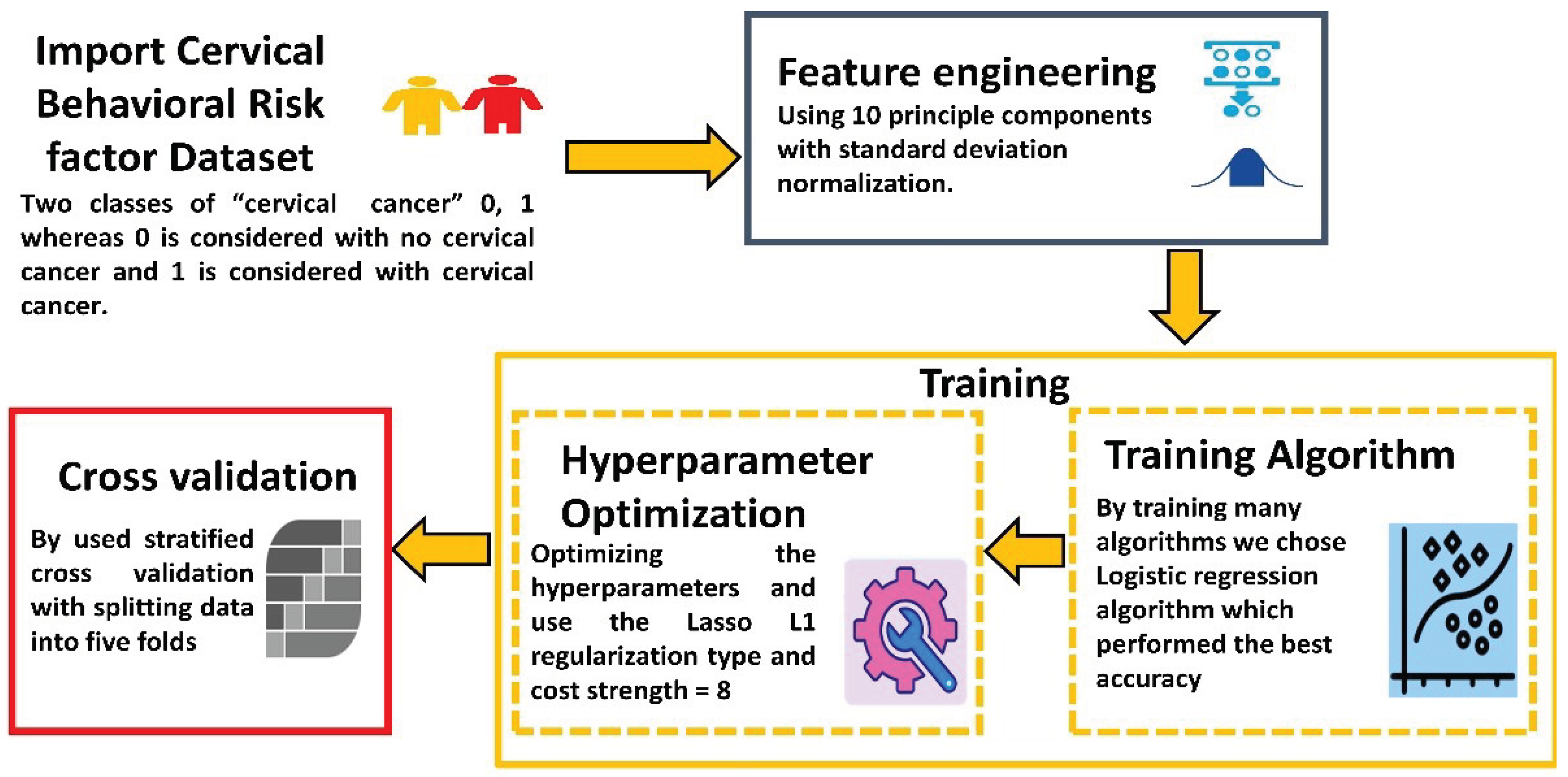
A framework for early prediction of cervical cancer based on behavioral risk factors was developed using a data mining tool. As shown in Error! Reference source not found., we performed four main stages using a data mining tool. At first, we imported the dataset and then used post processing techniques [30]. After that, we chose the logistic regression algorithm, optimized the hyperparameter, and finally trained the algorithm using the stratified K-fold cross technique (Table 2).

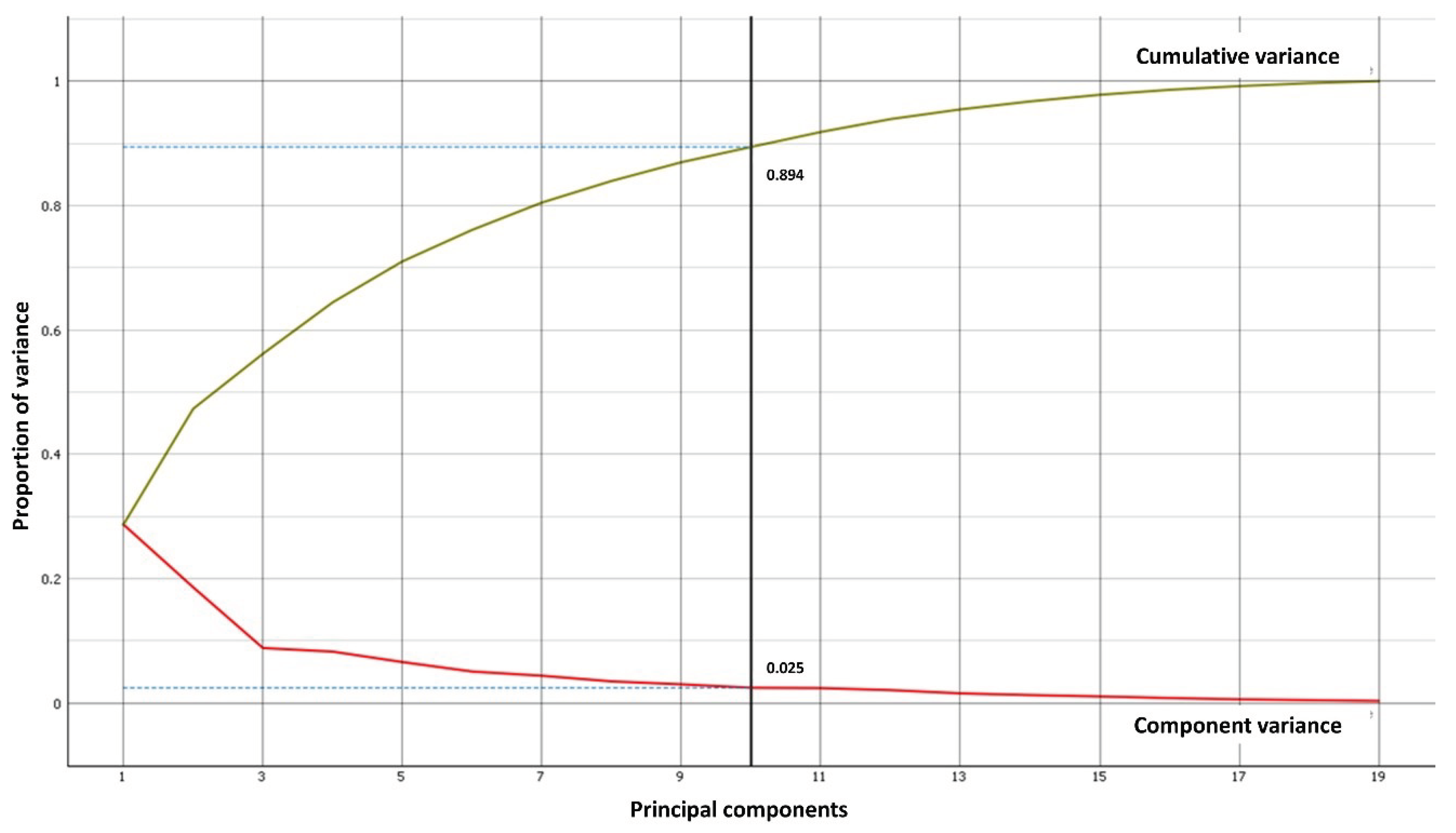
In the first stage, we imported the dataset. The dataset we used (Cervical Cancer Behavior Risk Data Set) was obtained from the UCI Machine Learning Repository website [31] and it is publicly available. This dataset contains seventy-two instances. It includes nineteen attributes with two classes of “ca_cervix” is 0, 1 where 0 is considered with no cervical cancer and 1 is considered with cervical cancer. There was no missing value to deal with, and all the attributes including the class variable, were int64 format, so it is noteworthy to mention that we didn't need encoding. In the second stage, the feature engineering and preprocessing procedure started to help in optimizing the outcome results in high quality as we used principal component analysis (PCA) [32]. PCA was employed to make feature reduction that uses an orthogonal transformation to turn correlated features into linearly uncorrelated features by compressing the selected features to 10 principal components with standard deviation normalization which covered 89% of the variance in features as shown in Figure 2.

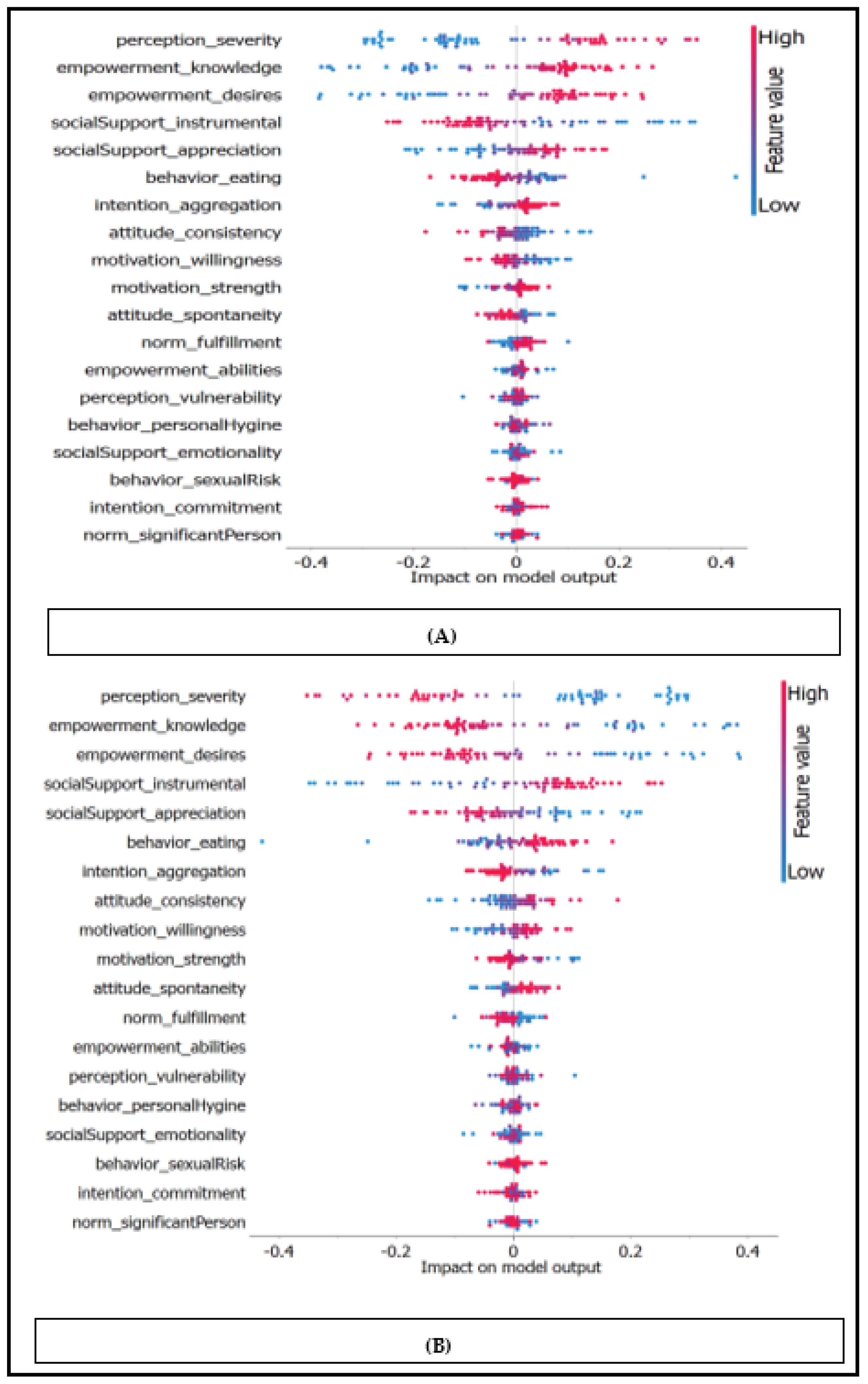
The Scree Diagram is a graph that the Principal Component Analysis (PCA) widget displays, as depicted in Figure 2. The Scree Diagram is a useful tool in PCA as it shows the variation explained by each principal component. The key elements are arranged according to how much each factor explains. The diagram enables researchers to determine how many principal components that should retain for more investigation, that is the optimal number of primary components to retain when the eigenvalues begin to level off or decline. We can choose the number of principal components to employ in our study by analyzing the Scree Diagram. This can assist us in maintaining the key details while also simplifying the data. At this stage, we didn’t need to use feature selection techniques because as mentioned in L. Akter at al. study [4] which used the same dataset proved that the used dataset has no feature with a strong correlation with others and the maximum value of the correlation coefficient is 0.85 so there is no need to use feature selection techniques. Moreover, as shown in Figure 3, it explains model diagram which emphasized that the processed features have an important contribution to the output model. The Shapley Additive Explanations (SHAP) library's Explain Model widget describes the classification models and the effect of each feature on classification models (Figure 3). Using the Shapley Additive Explanations Package (SHAP), the Explain Model widget is a tool that aids in the explanation of regression and classification models. This widget uses SHAP values to show insights into the model's prediction process after receiving a trained model and reference data as input. A model's feature relevance can be measured uniformly using SHAP values. Each feature in a projection is given a value, indicating how much that feature contributed to the prediction as a whole. The Explain Model widget assists users in learning the factors that affect the model's predictions and provides them with insights into the model's behavior by examining these SHAP values. Explain Model widget offers a visual interface for examining and interpreting a model's SHAP values. Users can examine the overall feature relevance and interactively explore the contributions of various attributes to specific predictions. Understanding complex models and identifying any biases or problems with the model's decision-making process might also benefit from doing this.

In the third stage, we used the logistic regression algorithm [33] as it was the most suitable algorithm for such a problem. We have examined many algorithms but all of them were under an accuracy of 93%. The existing method i.e. L. Akter at al. study [4] as compared with our research study reached an accuracy of 93% so we excluded all the algorithms under 93% accuracy. In this stage, we optimized the hyperparameter to enhance the results. We used the Lasso L1 [34] regularization type and optimized the cost strength to 8. This parameter is the best parameter to enhance the logistic regression accuracy very well. In the last stage, we used stratified K cross-validation [35] to evaluate the results by taking 5 folds, and finally, the algorithm started for training. To the best of our knowledge, we could not find any research work in the literature that aims to increase the classification accuracy in the training process depending on the scientific base such as our work, and we are the first group to propose such a machine learning system.

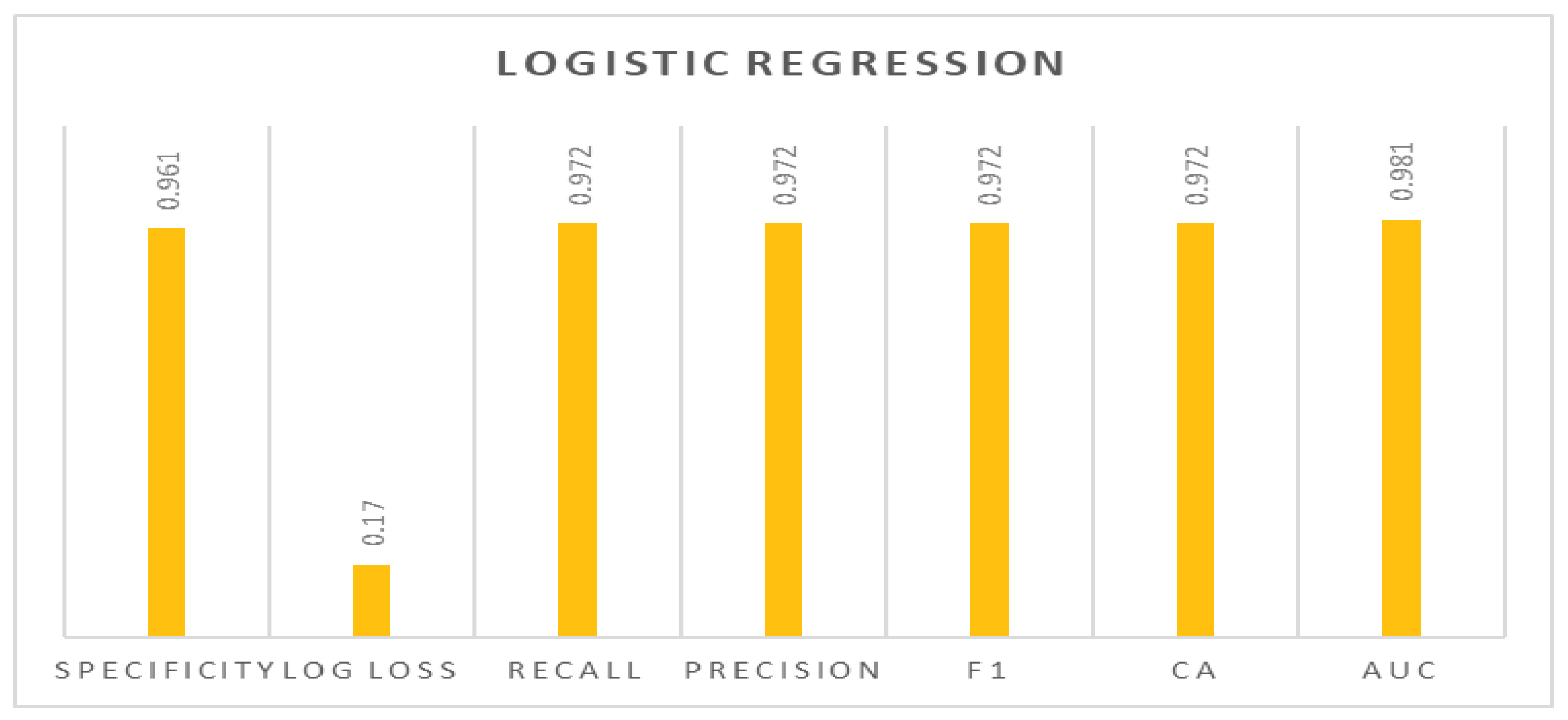
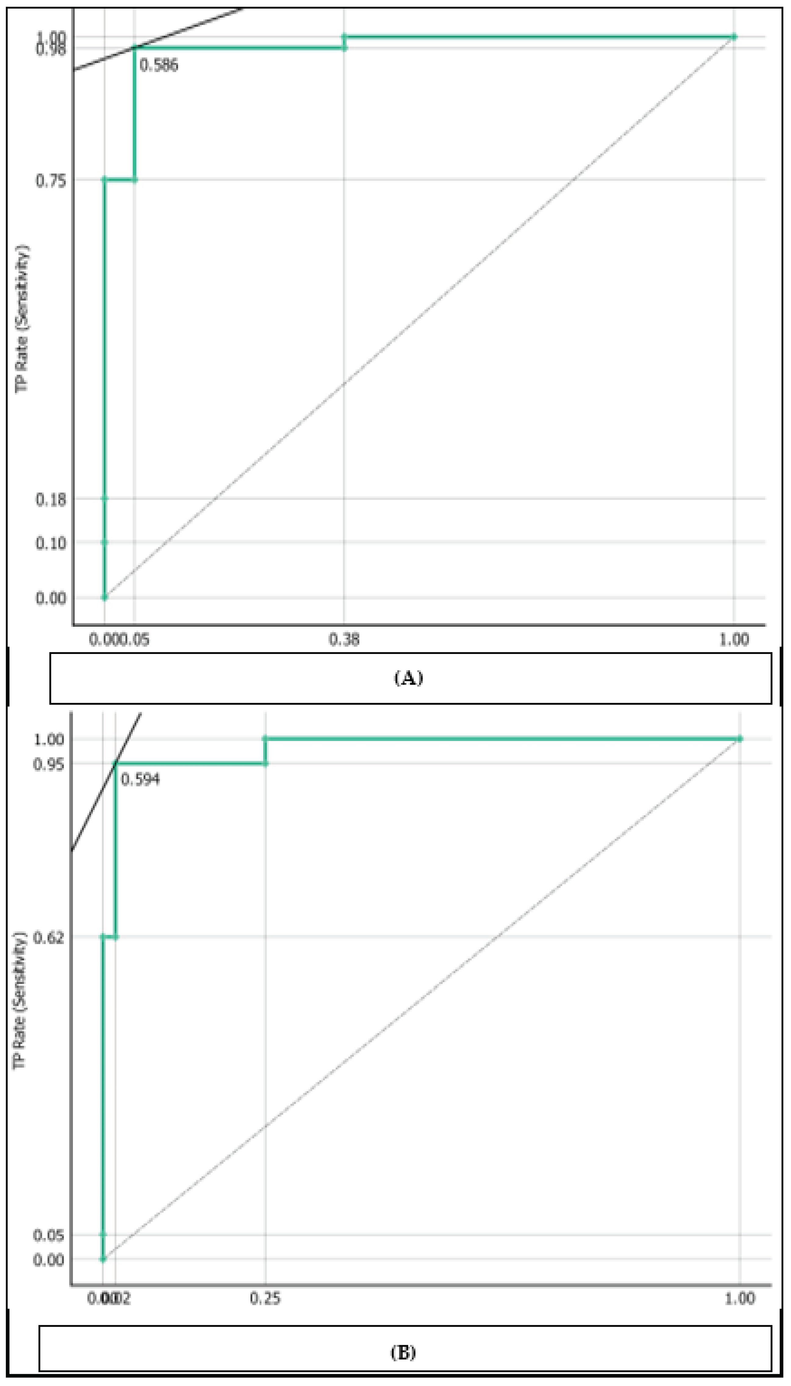
To predict and categorize the patient as having cervical cancer or not, we have applied many algorithms, however we excluded all the algorithms that are under 93% accuracy as we mentioned before. Therefore, we used the logistic regression in the training phase as it recorded promising results. We evaluated the effectiveness of our developed system using Classification Accuracy (CA), Area under the curve (AUC), precision, recall, specificity, log loss, and F1-score equations 1, 2, 3, 4, 5, and 6 as shown in Table 3. The confusion matrix of the logistic regression model with regularization type Lasso L1 which was the best regularization type used has been shown in Table 4. Table 5 and Table 6 respectively show the confusion matrix for logistic regression model with regularization type Ridge L2 and logistic regression model without regularization. The number of correctly classified instances was 50 for class 0 and 20 instances for class 1. However, the number of misclassified instances was 1 for class 0 and 1 instance for class 1. The accuracy of logistic regression with regularization type Lasso L1 with the best regularization type used was 97.2%, AUC is 98.1%, the F1 score is 97.2%, precision is 97.2%, recall is 97.2%, log loss is 17%, and specificity is 96.1% as shown in Table 3. The evaluated matrix of the proposed method is shown in Figure 4. The evaluated models may be seen on the Receiving Operator Characteristic (ROC) curve for classes 0 and 1 as shown in Figure 5. Moreover Figure 5 also shows the results of the testing classification algorithm. A visual tool for assessing the effectiveness of a classification model or diagnostic test is the Receiver Operating Characteristic (ROC) curve. The relationship between the true positive rate (sensitivity) and the false positive rate (specificity) at various categorization thresholds is represented visually. It enables readers to comprehend the trade-off between sensitivity and specificity and select the best classification threshold that complies with our distinctive requirements. where FP, FN, TN and TP denote the counts of false positive, false negative, true negative and true positive, respectively. where N denotes the number of rows in the test set, while M is the number of fault delivery classes, and $p_{ij}$is the predicted probability that the observation belongs to class j.

Using comprehensive techniques has increased the accuracy and performance of our model compared with existing methods. First, using principal component analysis (PCA) is a feature engineering technique that focuses on reducing dimensionality to help shorten training time and improve the data compatibility with the learning model class. Several machine learning models must be trained, and PCA is a critical step in this process. PCA assists in simplifying the complexity of the data while maintaining the most crucial information by lowering the dimensionality of a dataset. PCA enables the model to concentrate on the most important variables by identifying and deleting redundant or irrelevant features, improves accuracy, expedites training, and improves generalization as well. In essence, PCA serves as a potent tool for data preprocessing that makes it possible to train models quickly and effectively. This reflects on the accuracy of model while using PCA. Table 7 shows the difference in accuracy while using PCA and without using PCA among logistic regression models. It seems that PCA helped in improving accuracy very well. Since it enables the model to closely fit the training data without any constraints, it appears that logistic regression without regularization and without PCA could occasionally provide more accurate results. Nevertheless, this could result in overfitting, where the model performs well with training data but poorly with fresh or untested data. However, by introducing a penalty for high coefficients, regularization in logistic regression helps prevent overfitting. As a result, the accuracy may be slightly less accurate as compared to the non-regularized model. The accuracy of the model may also be impacted by the removal of certain crucial information from the data when applying PCA for dimensionality reduction. Thus, when deciding between these methods, it's crucial to strike a balance between precision and overfitting.

We selected the number of principal components depending on the specific area of application and the specific data set. However, we used the visual examination of a scree plot approach to determine the number of principal components [36]. Using a scree plot to determine the number of principal components is a common approach, by scanning the scree plot for a point where the amount of variance explained by each subsequent principal component begins to decline. In the scree plot, this is commonly referred to as an elbow as shown in Figure 2.

Table 9 shows the accuracy of different numbers of principal components.

Table 9 reveals that using 10 PCA is the best number of component analyses which leads to the best accuracy. Furthermore, using a strong classifier with optimization has incredibly improved results very well. One of the most powerful techniques that helped to increase the accuracy is logistic regression (LR). LR is used for binary classification problems, and it contains more than one powerful technique designed for increased accuracy. One of the most important optimizations of logistic regression provided is regularization. Regularization is applying a penalty to increase the magnitude of parameter values to reduce overfitting. It helps in minimizing the error between what the model predicts for the dependent variable given in the data compared to what the dependent variable is. The problem begins when several parameters existed but not too much data. In this case, the model will often tailor the parameter values to be specific for the data which means it fits the data almost perfectly. However, because this pattern doesn’t appear in future data, the model will predict poorly. To solve this problem and enhance results and accuracy we used lasso regression, (Least Absolute Shrinkage, and Selection Operator) add this function which penalizes large values of the parameters to what is already minimized to help in a better accurate prediction. The added function is λ |θj|, which is some constant λ multiplied by the sum of the absolute value of the magnitude of the coefficient which values are θj where the strength cost C = 1/λ [37]. As shown, Table 8 emphasized that optimizing the strength of cost C to 8 achieved good accuracy. Moreover, in this type of regularization, the logistic regression cost function gains a penalty term from Ridge L2 regularization that is inversely related to the square of the magnitude of the coefficients. The coefficients are not required to be exactly zero, but this penalty term encourages them to be minimal. As a result, Ridge L2 regularization frequently causes the coefficients to drop towards zero but infrequently causes them to disappear totally. A penalty term that is proportionate to the absolute value of the coefficients is added to the cost function by lasso L1 regularization, on the other hand. Lasso L1 regularization, in contrast to Ridge L2 regularization, has the ability to carry out feature selection by bringing some coefficients to a precise zero value. In other words, Lasso L1 regularization can successfully remove pointless features from the model, resulting in a more comprehensible and sparse solution. "Vanilla" logistic regression is logistic regression that has not undergone any regularization. The model seeks to minimize the negative log-likelihood of the observed data and there is no additional penalty term added to the cost function. Logistic regression may be prone to overfitting if regularization is not used, especially when there are many characteristics relative to the number of observations. Some coefficients might become zero and get eliminated from the model which helps in feature selection. Moreover, coefficient values are closer to zero when the penalties are higher (ideal for producing simpler models). In contrast, coefficients are not eliminated when using Ridge regression L2 regularization. As a result, when compared to the Ridge regression and Lasso regression, the Lasso Regression is much simpler to understand and gives high accuracy [38] as shown in Table 8. Moreover, as shown in Table 10, the existing method 1 [4] which are compared with our study used three different classification algorithms on the same dataset to evaluate their performance in detecting cervical cancer depending on the behavioral risk factors reaching 93 % for each classifier. However, they didn’t use PCA. Furthermore, the existing method 2 [24] which used the same dataset reached an accuracy of 91.6% for the Naive Bayes classifier and an accuracy of 87.5% for the logistic regression algorithm. These results have definitely proved the validity and strength of our proposed method.

In closure, its crucial to mention that innovative cervical malignant growth screening method is a key component of the prevention campaign that will eventually reduce the variance in cervical disease rates across the globe. To effectively eliminate cervical cancer, concerned administrations must engage women at the local level with initiatives that are sufficient, affordable, user-friendly, and sustainable programs. In this study, we proposed a high-performing machine learning approach to detect the cervical malignant development hazard structure at earlier stages based on behavioral risk factors. We have displayed the logistic regression classifier performance using several measures including AUC, accuracy, precision, log loss, specificity, recall, and F1-score. The accuracy rate for the logistic regression was 97.2%. Finally, we included feature engineering techniques for dimension reduction and optimizing the accuracy measures.

References

1. Johnson, C.A.; James, D.; Marzan, A.; Armaos, M. Cervical Cancer: An Overview of Pathophysiology and Management. Semin. Oncol. Nurs. 2019, 35, 166–174. [Google Scholar] [CrossRef]
2. Hussain, S.A.; Sullivan, R. Cancer Control in Bangladesh. Ultrasound Med. Biol. 2013, 43, 1159–1169. [Google Scholar] [CrossRef]
3. Hull, R.; Mbele, M.; Makhafola, T.; Hicks, C.; Wang, S.M.; Reis, R.M.; Mehrotra, R.; Mkhize-Kwitshana, Z.; Kibiki, G.; Bates, D.O.; Dlamini, Z. Cervical cancer in low and middle-income countries. Oncology letters 2020, 20, 2058–2074. [Google Scholar] [CrossRef]
4. Akter, L.; Islam, F.A.; Islam, M.; Al-Rakhami, M.S.; Haque, R. Prediction of Cervical Cancer from Behavior Risk Using Machine Learning Techniques. SN Comput. Sci. 2021, 2, 1–10. [Google Scholar] [CrossRef]
5. W. India, “Guidelines for Cervical Cancer Screening Programme,” 2006.
6. Denny, L.; de Sanjose, S.; Mutebi, M.; O Anderson, B.; Kim, J.; Jeronimo, J.; Herrero, R.; Yeates, K.; Ginsburg, O.; Sankaranarayanan, R. Interventions to close the divide for women with breast and cervical cancer between low-income and middle-income countries and high-income countries. Lancet 2016, 389, 861–870. [Google Scholar] [CrossRef]
7. Zhang, S.; Xu, H.; Zhang, L.; Qiao, Y. Cervical cancer: Epidemiology, risk factors and screening. Chinese Journal of Cancer Research 2020, 32, 720. [Google Scholar] [CrossRef] [PubMed]
8. Kashyap, N.; Krishnan, N.; Kaur, S.; Ghai, S. Risk Factors of Cervical Cancer: A Case-Control Study. Asia-Pacific J. Oncol. Nurs. 2019, 6, 308–314. [Google Scholar] [CrossRef]
9. Paul, S.B.; Tiwary, B.K.; Choudhury, A.P. Studies on the epidemiology of cervical cancer in Southern Assam. Assam University Journal of Science and Technology 2011, 7, 36–42. [Google Scholar]
10. Ebrahim, S.H.; Anderson, J.E.; Weidle, P.; Purcell, D.W. Race/Ethnic Disparities in HIV Testing and Knowledge About Treatment for HIV/AIDS: United States, 2001. AIDS Patient Care STDs 2004, 18, 27–33. [Google Scholar] [CrossRef] [PubMed]
11. Bergen, J.E.A.M.v.; Hoenderboom, B.M.; David, S.; Deug, F.; Heijne, J.C.M.; van Aar, F.; A Hoebe, C.J.P.; Bos, H.; Dukers-Muijrers, N.H.T.M.; Götz, H.M.; et al. Where to go to in chlamydia control? From infection control towards infectious disease control. Sex. Transm. Infect. 2021, 97, 501–506. [Google Scholar] [CrossRef] [PubMed]
12. Huang, J.; Deng, Y.; Boakye, D.; Tin, M.S.; Lok, V.; Zhang, L.; Lucero-Prisno, D.E.; Xu, W.; Zheng, Z.-J.; Elcarte, E.; et al. Global distribution, risk factors, and recent trends for cervical cancer: A worldwide country-level analysis. Gynecol. Oncol. 2021, 164, 85–92. [Google Scholar] [CrossRef]
13. Zhang, S.; Xu, H.; Zhang, L.; Qiao, Y. Cervical cancer: Epidemiology, risk factors and screening. Chinese Journal of Cancer Research 2020, 32, 720. [Google Scholar] [CrossRef] [PubMed]
14. Ashok, B.; Aruna, P. Comparison of Feature selection methods for diagnosis of cervical cancer using SVM classifier. Int. J. Eng. Res. Appl 2016, 6, 94–99. [Google Scholar]
15. Osuwa, A.A.; Oztoprak, H. Importance Of Continuous Improvement of Machine Learning Algorithms From A Health Care Management And Management Information Systems Perspective. In Proceedings of the 2021 International Conference on Engineering and Emerging Technologies (ICEET), Istanbul, Turkey, 27–28 October 2021; pp. 1–5. [Google Scholar]
16. Kaur, P.; Singh, G.; Kaur, P. Intellectual detection and validation of automated mammogram breast cancer images by multi-class SVM using deep learning classification. Informatics in Medicine Unlocked 2019, 16, 100151. [Google Scholar] [CrossRef]
17. Conner, M.; Sparks, P. Theory of planned behaviour and health behaviour. Predicting health behaviour 2005, 2, 121–162. [Google Scholar]
18. Webb, T.L.; Sheeran, P. Does changing behavioral intentions engender behavior change? A meta-analysis of the experimental evidence. Psychol. Bull. 2006, 132, 249–268. [Google Scholar] [CrossRef] [PubMed]
19. Conner, M. Cognitive determinants of health behavior. Handbook of behavioral medicine: Methods and applications, 2010; pp.19-30.
20. Fitch, J.L.; Ravlin, E.C. Willpower and perceived behavioral control: Influences on the intention-behavior relationship and postbehavior attributions. Soc. Behav. Pers. Int. J. 2005, 33, 105–124. [Google Scholar] [CrossRef]
21. Dillard, J.P. An Application of the Integrative Model to Women's Intention to Be Vaccinated Against HPV: Implications for Message Design. Heal. Commun. 2011, 26, 479–486. [Google Scholar] [CrossRef] [PubMed]
22. Larkey, L. Las Mujeres Saludables: Reaching Latinas for Breast, Cervical and Colorectal Cancer Prevention and Screening. J. Community Heal. 2006, 31, 69–77. [Google Scholar] [CrossRef]
23. Luszczynska, A.; Durawa, A.B.; Scholz, U.; Knoll, N. Empowerment Beliefs and Intention to Uptake Cervical Cancer Screening: Three Psychosocial Mediating Mechanisms. Women Heal. 2012, 52, 162–181. [Google Scholar] [CrossRef]
24. Sobar; Machmud, R. ; Wijaya, A. Behavior Determinant Based Cervical Cancer Early Detection with Machine Learning Algorithm. Adv. Sci. Lett. 2016, 22, 3120–3123. [Google Scholar] [CrossRef]
25. Asadi, F.; Salehnasab, C.; Ajori, L. Supervised Algorithms of Machine Learning for the Prediction of Cervical Cancer. J. Biomed. Phys. Eng. 2020, 10, 513–522. [Google Scholar] [CrossRef]
26. Deng, X.; Luo, Y.; Wang, C. November. In Analysis of risk factors for cervical cancer based on machine learning methods. In Proceedings of the 2018 5th IEEE international conference on cloud computing and intelligence systems (CCIS), Nanjing, China, 23–25 November 2018; pp. 631–635. [Google Scholar]
27. Nithya, B.; Ilango, V. Evaluation of machine learning based optimized feature selection approaches and classification methods for cervical cancer prediction. SN Appl. Sci. 2019, 1, 641. [Google Scholar] [CrossRef]
28. Tseng, C.-J.; Lu, C.-J.; Chang, C.-C.; Chen, G.-D. Application of machine learning to predict the recurrence-proneness for cervical cancer. Neural Comput. Appl. 2013, 24, 1311–1316. [Google Scholar] [CrossRef]
29. Suman, S.K.; Hooda, N. Predicting risk of Cervical Cancer : A case study of machine learning. J. Stat. Manag. Syst. 2019, 22, 689–696. [Google Scholar] [CrossRef]
30. Dai, D.; Xu, T.; Wei, X.; Ding, G.; Xu, Y.; Zhang, J.; Zhang, H. Using machine learning and feature engineering to characterize limited material datasets of high-entropy alloys. Comput. Mater. Sci. 2020, 175, 109618. [Google Scholar] [CrossRef]
31. “UCI Machine Learning Repository: Cervical Cancer Behavior Risk Data Set.” (Accessed Sep. 08, 2022).
32. Gewers, F.L.; Ferreira, G.R.; Arruda, H.F.D.; Silva, F.N.; Comin, C.H.; Amancio, D.R.; Costa, L.D.F. Principal component analysis: A natural approach to data exploration. ACM Computing Surveys (CSUR) 2021, 54, 1–34. [Google Scholar] [CrossRef]
33. Connelly, L. Logistic regression. Medsurg Nursing 2020, 29, 353–354. [Google Scholar]
34. Camur, M.C.; Ravi, S.K.; Saleh, S. Enhancing supply chain resilience: A machine learning approach for predicting product availability dates under disruption. Expert Syst. Appl. 2024, 247. [Google Scholar] [CrossRef]
35. Prusty, S.; Patnaik, S.; Dash, S.K. SKCV: Stratified K-fold cross-validation on ML classifiers for predicting cervical cancer. Front. Nanotechnol. 2022, 4. [Google Scholar] [CrossRef]
36. Deliu, G.; Miron, C.; Opariuc-Dan, C. Item Dimensionality Exploration by Means of Construct Map and Categorical Principal Components Analysis. J. Balt. Sci. Educ. 2019, 18, 209–226. [Google Scholar] [CrossRef]
37. Shcherban, S.; Liang, P.; Tahir, A.; Li, X. Automatic identification of code smell discussions on stack overflow: A preliminary investigation. In Proceedings of the 14th ACM/IEEE international symposium on empirical software engineering and measurement (ESEM), 1–6. 2020. [Google Scholar]
38. Sudhaman, K.; Akuthota, M.; Chaurasiya, S.K. A Review on the Different Regression Analysis in Supervised Learning. Bayesian Reasoning and Gaussian Processes for Machine Learning Applications 2022, 15–32. [Google Scholar]
Figure 2. The scree diagram shows the degree of variance which covered by the best principal component number.
Preprints 101828 g002
Figure 3. The SHAP library's Explain Model widget provides a description of the classification model. (A) Impact on output model for class 0. (B) Impact on output model for class 1.
Preprints 101828 g003
Figure 4. The logistic regression "Lasso regression" type evaluated matrices chart describe the percentage of the accuracy, precision, specificity, recall, log loss, the F1 score, and the area under curve (AUC).
Preprints 101828 g004
Figure 5. The Receiving operator characteristic (ROC) to show the relationship between the true positive rate (sensitivity) and the false positive rate (specificity). (A) ROC curve for class 0. (B) ROC curve for class 1.
Preprints 101828 g005