Do Central Banks Respond to Exchange Rate Movements? A Structural Analysis of Selected Inflation Targeters Emerging Economies

Preprint

Article

Do Central Banks Respond to Exchange Rate Movements? A Structural Analysis of Selected Inflation Targeters Emerging Economies

Altmetrics

Downloads

145

Views

Comments

Christian Kakese Tipoy^*

This version is not peer-reviewed

Submitted:

22 March 2024

Posted:

25 March 2024

You are already at the latest version

Alerts

Abstract

We analyze whether the central banks of a selected sample of emerging economies respond to exchange rate movements. We use economies that are inflation targters and exporters of a limited number of commodities. The latter renders them vulnerable to terms of trade shocks. The sample comprises Brazil, the Czech Republic, India, Indonesia, Russia and South Africa. We also investigate the role played by the terms of trade in explaining their business cycles. We estimate, for each economy separately and using Bayesian techniques, a regime switching open new Keynesian model. This model allows the parameters of the policy rule and the structural shocks to switch between periods of low and high regimes. We perform posterior simulation and find that, when compared to a constant parameters model, the regime switching fits the data better. The results indicate that, in some periods, the different economies respond strongly to exchange rate, while in others, some respond weakly. A terms of trade improvement leads to a currency appreciation. However, this is reversed for those economies that respond strongly to exchange rate movements. This leads to a rise in output and inflation even for economies that do not respond strongly but play a major role in international trade. This is the case of Russia. The terms of trade are found to play a major rule in explaining business cycles in emerging economies. Thus, although these economies follow an inflation targeting framework, they may set their respective policy rate in a manner to take into account exchange rate developments. This insulates themselves against adverse terms of trade shocks.

Keywords:

Subject: Business, Economics and Management - Economics

1. Introduction

There is a tendency for central banks to react to exchange rate movements despite adopting a flexible exchange rate regime. Indeed, Levy-Yeyati and Sturzenegger [1] note that several countries that have a flexible regime intervene in the market to influence their exchange rates. This creates a wedge between the "de jure" and the "de facto" regimes.1 This observation may also be true for economies that have adopted the Inflation Targeting (IT) framework despite the requirement that precludes the targeting of other indicators such as wages, the level of employment and the exchange rate [see [2]. Emerging economies may be tempted to respond to exchange rate movements. Indeed, they are characterised by higher volatility. Their trade balances to output ratio are significantly more countercyclical. Given that they are small economies that export a limited number of commodities, foreign shocks such as the terms of trade are an important source of domestic business cycles fluctuations [3,4]. Their export earnings are highly unstable due to frequent and sharp fluctuations in international prices of their commodities [5]. Therefore, exchange rate movements pose a risk when balancing the objectives of price stability and economic growth, hightening the necessity of an explicit role for it in monetary policy [6]. Alstadheim et al. [7] opine that commodities exporters have an incentive in altering their exchange rates given their volatile terms of trade.

Do central banks set their policy rates to respond to exchange rate movements? The results are mixed.2 Lubik and Schorfheide [3] estimate a constant parameters dynamic stochastic general equilibrium (DSGE) model for Australia, Canada, New Zealand and the United Kingdom (UK). They find that only the central banks of Canada and UK react to exchange rate movements. However, using the same set of economies and a DSGE model that incorporates nominal and real frictions, [6] finds that these economies do not react to exchange rate movements. Alstadheim et al. [7] add Norway and Sweden to the previous set. They estimate a regime switching DSGE model and find that the policy parameters and the volatility of the structural shocks have not remained constant. In some periods, the respective central banks respond to exchange rates fluctuations while in others, some do not. For emerging economies, Mohanty and Klau [8] estimate a Taylor rule for a sample of emerging economies. They find that, in general, the central banks react to exchange rate volatility. For some central banks, the goal of exchange rate stability tends to supersede those of inflation and output stability. Ortiz and Sturzenegger [9] and Alpanda et al. [10] estimate a constant parameters DSGE model for the South African economy. They both find that no explicit weight is put on currency depreciation.

We analyze whether the central banks of a sample of emerging economies respond to exchange rate fluctuations. We focus on economies that have adopted the IT as their monetary policy framework.3 These economies are expected to follow, at least in the "de jure" sense, a flexible exchange rate regime. However, given that they export a limited number of commodities, they may have an incentive to smooth exchange rates. The sample comprises Brazil, the Czech Republic, India, Indonesia, Russia and South Africa. We use an open DSGE model in the spirit of Lubik and Schorfheide [11] and Gali and Monacelli [12]. The model is estimated, using quarterly data and Bayesian techniques, separately for each economy. As in Alstadheim et al. [7], we allow the parameters of the policy rule and the volatility of the structural shocks to switch endogenously between low and high regimes. Indeed, economies go through regime changes and shift in volatility that a constant parameters model will fail to capture. We conduct a posterior simulation of a constant parameters and a regime switching model; and compute the log marginal data density based on the Laplace approximation. We find that the regime switching model fits the data better. The estimation results indicate that both policy parameters and volatility of the structural shocks have not remained constant. All these economies respond to exchange rate movements, at various degrees, in both low and high regimes. The Czech Republic has the strongest response in both regimes. In the high regime, an exchange rate deviation from its target leads the Czech central bank to raise the interst rate by more than the deviation. South Africa has the second highest response in the high regime, followed by India, Indonesia and Russia. Altough Brazil has a moderate response to exchange rate deviation, the country has the second strongest response in the low regime, followed by South Africa. India, Indonesia and Russia put a meager weight on exchange rate in the low regime. Interestingly, we also find that the Czech Republic is the most opened economy. Contrary to Alstadheim et al. [7]’s findings, these emerging economies respond strongly to inflation too, highlighting the importance of both price and exchange rate stability. Following a terms of trade improvement, we find that the currency appreciation is reversed for economies that respond strongly to exchange rate movements. This reversal, for economies like the Czech Republic, spurs output and inflation. However for economies that play a major role in international trade, like Russia, output rises despite the strong currency appreciation. The variance decompositions show that the terms of trade play a major role in explaining the various domestic business cycles. This provides an incentive to emerging economies to smooth exchange rates.

The remainder of this article is organized as follows. In section 2, we look at some stylized facts of these emerging economies. In section 3, we present the regime switching DSGE model. The data and Bayesian estimation are covered in section 4 while the results are discussed in section 5. Section 6 concludes this article.

2. Some stylized facts

The emerging economies considered in this article, as stated previously, are inflation targeters and commodities exporters. These economies have used, prior to the IT adoption, various monetary frameworks ranging from monetary aggregates to exchange rates targeting. As a commonality, they all have a history of high inflation and other imbalances.

The Republic of Brazil went through a series of policy changes following the poor economic performances of the 1980’s and early 1990’s. During this period, the country experienced external financing problems, accelerating inflation and economic stagnation [13]. In the mid 1980’s, inflation stood above 200% due to poor policies and measures taken to generate trade surpluses [14]. In 1994, the establishment of the "Real Plan", a stabilization programme with the aim of curbing the past poor performance; led to a fall of inflation, reaching an average of 1% in 1996 [15]. However, following strong pressures on foreign exchange reserves, the country moved from a crawling peg to a flexible exchange rate in January 1999. This move signaled the adoption of the IT framework that came in mid-1999 [16].

The Czech Republic had a monetary policy centered on a fixed exchange rate regime and monetary aggregates targeting before the IT adoption. The country managed to maintain a stable exchange rate owing to low capital inflows and met the monetary targets. In the mid 1990’s, inflationnary pressures grew up due to the rise of capital flows. This weakened economic growth and monetary policy had to be tightened. Following am exchange rate crisis and a severe recession in 1997, the fixed exchange rate regime had to be abandonned. In late 1997, the IT framework was adopted with the goal of achieving an inflation rate between 3.5%-5.5% by the end of the year 2020 [see [17].

In 1985, India adopted a monetary targeting framework with feedback following a period where policy was centered on credit regulation. The growth rate of broad money was used as the intermediate target and projected in a manner consistent with expected GDP growth and some acceptable inflation rate [18]. However, money demand became unstable in the 1990’s due to the liberalization of the financial market and the increase in the country’s openess. In 1998, the country moved to a multiple indicators approach that includes all economic and financial variables having an influence on monetary policy objectives. In 2015, the parliament of India mandated the Reserve Bank to pursue an IT framework, with the target sets at 4% with a band of 2% - 6%. The arrangement came into effect in August 2016, with the country making a formal transition towards a flexible IT [19]. Since the adoption, the inflation rate has remained generally within the band [20].

The primary mandate of the central bank of Indonesia is to achieve and maintain the stability of the country’s currency. This mandate encompasses both price and exchange rate stability. The act of 1999 sets the independence of the Bank of Indonesia and provided a basis for the application of the IT framework [21,22]. This was following years of high inflation. Indeed, in the 1980’s, inflation stood at 9.40% on average before falling at 8.65% between 1990 and 1997 [23]. From the year 2000, the country used a form of IT with the base money as the operating target [see [24] before formally adopting it in July 2005.

Russia experienced several years of high inflation, especially pre-2000. In the early 1990’s, the heritage of the central planning, among other factors, rendered inexistant an effective monetary policy framework [25]. In 2012, the inflation rate came down to 5.1% from a staggering 8.4% in the previous year. However, due to economic sanctions and low oil prices, it rose to 6.8% in 2014. This led the Russian central bank to move from an exchange rate targeting to an IT in June 2014. However, the framework was officialy adopted in 2015, with the goal of reducing inflation and keeping it close to a target of 4%. This higher target, compared to most countries, was justified by the high and unanchored inflation expectations; and the necessity of mitigating the risk of deflationary trends. The Russian monthly inflation rate fell to an average of 3%, year on year, in 2017 from a 15% in 2015 [26]. Due to the late international sanctions following the war in Ukraine, inflation has risen, reaching 15%.

South Africa’s monetary policy was focused on various indicators before the adoption of the IT framework. The central bank used, among others regimes, the bank credit extension, the exchange rate and the monetary aggregate targeting [27]. The country moved to a formal IT framework in 2000 with the aim of keeping inflation within a target range of 3-6%. Since its adoption, Mandeya and Ho [28] stress that inflation has significantly decreased from an average of 9.4%, before the adoption, to 5.3%. Despite this reduction, the inflation rate has lingered over the target range for some periods. In the early years of the adoption and between 2007-2009, the country recorded an inflation rate above the upper target [29].

We can note from the previous facts some key elements. Firstly, these economies have witnessed episodes of high inflation prior the adoption of the IT. The move to this framework has coincided with a sensible reduction of inflation. Indeed, Fraga et al. [30] indicate that countries that have adopted the IT have managed to lower significantly their inflation rates. Secondly, the announcement of the move to the IT does not coincide with its actual adoption. Certain economies have introduced gradually this new monetary policy framework. Lastly, some economies have used some forms of monetary frameworks, such as the exchange rate targeting, in conjonction with the IT. These facts make it is too restrictive to assume that both policy parameters and volatility of structural shocks have remained constant during the entire sample.

We present in Table 1 the volatility of some key variables before and after the official adoption of the IT framework.4 Not all economies have managed to reduce their inflation volatility after the adoption of the IT framework. Indeed, Indonesia and Russia have recorded a rise although not substantial. India is the only economy that has recorded a fall of exchange rate volatility although meagre after the IT move. A quick comparison with the other variables shows that exchange rate has the lowest volatility. This result supports the "fear of floating" that characterises emerging economies. Holland [31] considers a lower exchange rate volatility relative to the interest rates one as a proof of exchange rate intervention. Russia and South Africa are the only two economies to record a fall of terms of trade volatility. Except for India, the remaining economies have not only a sizable output volatility but also have faced a rise after the IT adoption. Again, these changes in volatility will make the constant parameters model too restrictive.

The previous facts support the regime switching model as the appropriate framework to capture both changes in the policy parameters and in the volatility of the structural shocks. Even a strategy that splits the sample into two will be difficult to implement. Indeed, the dates of the announcement of the move to the IT framework do not necessarily correspond to its actual adoption and implementation. The facts also highlight the changes in volatility that have occured during the entire sample. Moreover, although the low exchange rate volatility may suggest some intervention in the foreign exchange market, central banks may also respond on and off to exchange rate deviation. In the next section, we present the model and the estimation framework.

3. A regime switching DSGE model

3.1. The model

The model is an open new Keynesian DSGE along the work of Gali and Monacelli [12] and Lubik and Schorfheide [3]. It is extended to accomodate regime switching in both the parameters of the monetary policy rule and the volatility of the structural shocks as in Alstadheim et al. [7]. The open IS curve is given by the following expression (1) :

y_{t} = E_{t} y_{t + 1} - (τ + λ) (i_{t} - E_{t} π_{t + 1}) - ρ_{z} z_{t} - α (τ + λ) E_{t} Δ q_{t + 1} + \frac{λ}{τ} E_{t} Δ y_{t}^{*} + ε_{t}^{y};

(1)

where

y_{t}

is output,

i_{t}

is the nominal interest rate,

π_{t}

is inflation,

z_{t}

is the growth rate of a technological progress

A_{t}

q_{t}

is the terms of trade,

y_{t}^{*}

is the rest of the world output and

ε_{t}^{y}

is an autoregressive (AR) demand shock. In the same equation,

α

denotes the degree of openness,

τ

is the intertemporal elasticity of substitution and

λ = α (2 - α) (1 - τ)

. The exogenous processes

y_{t}^{*}

and

z_{t}

follow the AR processes given by:

\begin{matrix} y_{t}^{*} & = ρ_{y^{*}} y_{t - 1}^{*} + ε_{t}^{y^{*}}; \\ z_{t} & = ρ_{z} z_{t - 1} + ε_{t}^{z}; \end{matrix}

where

ε_{t}^{y *}

and

ε_{t}^{z}

are the respective exogenous shocks for world output and technology respectively. The different exogenous processes are

N (0, 1)

Equation (2) represents the open economy New Keynesian Phillips Curve (NKPC). It models the supply side of the economy and is expressed as:

π_{t} = E_{t} π_{t + 1} + α β E_{t} Δ q_{t + 1} - α Δ q_{t} + \frac{κ}{(τ + λ)} (y_{t} - {\bar{y}}_{t}) + ε_{t}^{π};

(2)

where

β

is the discount factor,

{\bar{y}}_{t} \equiv - α (2 - α) (1 - τ) / τ y_{t}^{*}

denotes potential ouput,

κ

is the structural slope of the NKPC as in Lubik and Schorfheide [3]; and

ε_{t}^{π}

is an AR domestic cost push shock.

The real exchange rate

s_{t}

is given by

s_{t} = Δ e_{t} - π_{t} + π_{t}^{*}

; where

π_{t}

and

π_{t}^{*}

denote domestic and world inflation respectively. Given that the real exchange rate is proportional to the terms of trade, we get the equation (3) below.

Δ e_{t} = π_{t} - (1 - α) Δ q_{t} - π_{t}^{*}

(3)

Following Lubik and Schorfheide [3] and Alstadheim et al. [7], the terms of trade are expressed as a law of motion of its growth rates.

Δ q_{t} = ρ_{q} Δ q_{t - 1} + ε_{t}^{q}

(4)

Monetary policy is conducted following a Taylor rule augmented by the nominal exchange rate depreciation. We not only analyze whether an economy responds to exchange rate depreciation, but also if it follows a strict or flexible IT framework. The Taylor rule is given by expression (5) below.

i_{t} = ρ_{i} (S_{t}^{P o l}) i_{t - 1} + (1 - ρ_{i} (S_{t}^{P o l})) (γ_{π} (S_{t}^{P o l}) π_{t} + γ_{y} (S_{t}^{P o l}) y_{t} + γ_{e} (S_{t}^{P o l}) Δ e_{t}) + ε_{t}^{i};

(5)

where

γ_{π}

γ_{y}

and

γ_{e} \geq 0

are the weights put on inflation, output and exchange rate respectively;

ρ_{i}

denotes the interest rate smoothing parameter and

ε_{t}^{i}

is the exogenous monetary policy shock. We allow the parameters of the Taylor rule to be governed by an independent two-states Markov process given by:

S_{t}^{P o l} \in {L o w, H i g h};

such that

(S_{t}^{P o l} = L o w) < (S_{t}^{P o l} = H i g h)

. According to this, the high response,

(S_{t}^{P o l} = H i g h)

, corresponds to the regime where the central bank responds strongly to the deviation of exchange rate depreciation from its target; while the low response,

(S_{t}^{P o l} = L o w)

, denotes the opposite. The Taylor rule parameters switch altogether albeit not necessarily in the same direction.

We allow the volatility of the different structural shocks to switch according to an independent two-states Markov process given by:

S_{t}^{V o l} \in {L o w, H i g h};

such that

(S_{t}^{V o l} = L o w) < (S_{t}^{V o l} = H i g h)

; where

(S_{t}^{V o l} = H i g h)

corresponds to the regime of high output volatility and

(S_{t}^{V o l} = L o w)

denotes the regime of low output volatility. Again, the different structural shocks do not switch necessarily in the same direction. Next, we look at the estimation strategy of the regime switching DSGE model.

3.2. The Markov switching rational expectation framework

The regime switching DSGE model, as in Maih [32], solves:

E_{t} \sum_{r_{t + 1} = 1}^{h} P_{r_{t}, r_{t + 1}} (I_{t}) {\tilde{d}}_{r_{t}} (x_{t + 1} (r_{t + 1}), x_{t} (r_{t}), x_{t - 1}, ε_{t}) = 0;

(6)

where

E_{t}

denotes the expectation operator,

{\tilde{d}}_{r_{t}} : R^{n_{v}} \to R^{n_{d}}

is a

n_{d} \times 1

vector of possibly nonlinear functions of their arguments,

r_{t} = 1, 2, \dots, h

is the regime at time t;

P_{r_{t}, r_{t + 1}} (I_{t})

is the transition probability from regime

r_{t}

in the current period to regime

r_{t + 1}

in the next period;

x_{t}

is a

n_{x}

vector of all endogenous variables; and

ε_{t}

denotes the

n_{ε}

vector of structural shocks. The transition probability is endogenous and a function of

(I_{t})

, the information set at time t. The solution of the problem is of the form:

x_{t} (r_{t}) = T^{r_{t}} (w_{t})

(7)

However, there is no solution in general to the problem given in (6). Therefore, we rely on a perturbation scheme, developped by Maih [32], to approximate the decistion rule in (7). This is done by inserting the functional form of the decision rule into (6) and its derivatives. The vector of the state variables is given by:

w_{t} \equiv {[x_{t - 1}^{'}, σ, ε_{t}^{'}]}^{'};

where

σ

denotes a perturbation parameter. The first order solution takes the form:

T^{r_{t}} (w) ≃ T^{r_{t}} ({\bar{w}}_{r_{t}}) + T_{w}^{r_{t}} (w_{t} - {\bar{w}}_{r_{t}});

(8)

where

{\bar{w}}_{r_{t}}

indicates the steady states values of the state variables in regime

r_{t}

. The solution is computed using the efficient Newton algorithm of Maih [32]. This framework allows the model to be in different regimes at different points in time and each regime is governed by a specific rule [7].

4. Data and Bayesian estimation

This article focuses on a sample of emerging economies that are commodities exporters and use the IT as their monetary policy framework. The emerging economies considered are Brazil, the Czech Republic, India, Indonesia, Russia and South Africa. The parameters of the model are estimated for each economy separately for a constant parameters and a regime switching model. All the estimations are conducted in Matlab using the Rationaliy In Switching Environments (RISE) toolbox of Maih [32].

4.1. Data

The differents models are estimated using quarterly data and the sample size for each economy depends on data availability.5 The data span from 1996Q2 to 2019Q4 for Brazil, 2000Q2 to 2019Q4 for both the Czech Republic and Indonesia, 1996Q2 to 2019Q4 for India, 1996Q2 to 2020Q4 for Russia and 1994Q2 to 2020Q4 for South Africa. The model for each economy comprises 7 observable variables: Real GDP, inflation, nominal short term interest rate, nominal effective exchange rates, terms of trade, foreign output and foreign inflation. All the data are from the FRED database of the Federal Reserve Bank of St Louis except the nominal effective exchange rates and the terms of trade.6 The nominal effective exchange rates series, in monthly frequency, are from the Bank of International Settlement (BIS) based on the country broad time-varying weights.7 The series are transformed into quaterly averages and the reciprocal computed so that an exchange rate increase indicates a currency depreciation. The terms of trade series, except for South Africa, are from the World Bank development indicators and transformed into quarterly frequency.8 The quaterly South African terms of trade series are from the South African Reserve Bank. Both foreign output and inflation are computed as a weighted average of the top three trading partners of each economy. We use the broad time-varying weights, rescaled to 100%, from the BIS. The foreign output is transfomed in percentage growth rates while foreign inflation is annualised. We compute the growth rates of GDP as the log differences of GDP in percentage. The inflation rates are the annualised log differences of CPI. The changes in terms of trade are computed as the log differences of terms of trade in percentage. The exchange rate depreciation is the log differences of the real effective exchange rates while the short term interest rate is used in percentage level.

4.2. Priors and estimation

To bring the model to the data, we relate the unobservable state variables and the observed variables, forming a state space model. For our constant parameters model, the Kalman filter allows the obtention of the unobserved state variables and the likelihood of the data. However, this is not feasible for our regime switching model. For this model, we follow Maih [32] who uses a modification of the [33]’s filter to compute an approximate likelihood.

With a likelihood at hands, we can now combine it with our priors to get a posterior. The priors are formulated using the quantiles of the different distributions. We consider the 90% probability intervals of these distributions and use loose priors for all the parameters, except the discount factor which is calibrated to 0.995.9 We then maximize the posterior to obtain the different modes. Due to the difficulty of sampling this posterior, we use the stochastic search approach of the Artificial Bee Colony (ABC) optimization to conduct posterior maximization. This optimization algorithm simulates the foraging behaviour of a bee colony [34,35]. We then simulate the posterior using the Random Walk Metropolis Hasting (RWMH) algorithm. We run two parallel Markov chains. For each chain, we make 210,000 draws, with a burnin of 10,000. We keep the 5th draw of each chain. We compute the log marginal data density (MDD) based on the Laplace approximation from the simulated posteriors. Each process is conducted separately for each economy and for both the constant parameters and the regime switching models.

5. Results

To answer our main question, we start by estimating a constant parameters model. In this model, both policy parameters and volatility of structural shocks are time invariant. However, as stated earlier, this constant model is too restrictive. Next, we estimate a regime switching DSGE model. In this model, the policy parameters and the volatility are allowed to switch between periods of low and high regimes. Although there is a possiblity of having more than two states, it has been seen that allowing only for two suits the data better (see Liu et al. [36], Debortoli et al. [37]. We contrast between these two models by comparing their log MDD.

5.1. Time invariant rational expectations

We estimate separetely for each economy the constant parameters DSGE model. Table 2 presents, in addition to the different priors, the posterior modes for the policy parameters and the volatility of the structural shocks. All the different economies pursue anti-inflationary policies given their large weights put on inflation. Moreover, they also react strongly to exchange rate deviation. The Czech Republic has the largest weight on exchange rate, followed by Russia and Brazil. All these economies, but the Czech Republic and Indonesia, respond strongly to output deviation too, with Russia having the largest response. For this latter economy, the goal of output stability tends to supersede those of price and exchange rate. These results are contrary to those of Alstadheim et al. [7] who find a weaker response to inflation deviation due to the inclusion of exchange rate in the Taylor rule. Our findings therefore highlight the importance of both price and exchange rate stability for emerging economies.

Looking at the structural shocks, the terms of trade have the largest volatility for India, Russia and South Africa. For these economies, this volatility is more than double of those of output and inflation. For Brazil, the Czech Republic and Indonesia, the terms of trade are among the top two largest volatility. These results indicate, as stressed by Uribe and Schmitt-Grohé [4], that the terms of trade are an important source of business cycles fluctuations for emerging economies. In the next section, we present the estimation results of our regime switching DSGE model.

5.2. Regime switching rational expectations

The constant parameters model is too restrictive as it does not take into account the changes in policy and volatility of structural shocks that may have occured. We therefore estimate a model with switches in policy parameters and in volatility for each economy separately. We first present the log MDD of the constant parameters and the regime switching model obtained using the Laplace approximation after posterior simulation. Table 3 presents the results of this exercise. We can note that the model with switches in parameters and volatility has the largest MDD compared to the constant model. Therefore, for each economy, the regime switching fits the data better than a constant parameters model. Next, we present and discuss the estimation results of this model.

The priors and the posterior modes for the regime switching model are reported in Table 4. The results indicate that the parameters of the policy rule have not remained constant. Starting with our parameter of interest, the response to exchange rate, the different central banks respond to its deviation at various degrees. The Czech Republic has the strongest response in both low and high regimes. In the high regime, this response is more than double of the remaining economies. South Africa, India, Indonesia and Russia are successively the next economies with a high response in the high regime. In the low regime, Indonesia and Russia have a weaker response. Despite having the weakest response in the high regime, Brazil has the second strongest response in the low regime after the Czech Republic. A quick comparison of the response to exchange rate with the results from the time invariant model indicates that the regime switching has larger weights, in the high regime, for India, Indonesia and South Africa. For the latter economy, the response in the low regime is still larger than the one of the time invariant model. Looking at the response to inflation deviation, despite the inclusion of the exchange rate in the policy rule, these economies respond strongly to a deviation. The weights on inflation, as in the time invariant model, obey the Taylor principle. Again, this is contrary to Alstadheim et al. [7]’s findings. The Czech Republic does not seem to respond strongly to inflation in the high regime. It is possible that by responding strongly to exchange rate, the Czech central bank may be succesful in insulating the economy from a terms of trade shock and stabilizing inflation. Therefore, the Czech central bank may not need a strong response to inflation deviation compared to the other economies. Indeed, Table 1 indicates that the Czech Republic has the lowest inflation and exchange rate volatility post-IT adoption. The response to inflation and exchange rate deviation supports the importance of both price and exchange rate stability for emerging economies. The goal of output stability is not neglected. Indeed, all these economies, but Brazil, respond strongly to output deviation in the high regime. However, for Brazil, the Czech Republic and India; the goal of exchange rate stability seems to supersede the one of output. Given these different responses, these economies do not follow a strict IT framework. There is a high degree of interest rate smoothing for all these economies in both regimes. This indicates that financial stability is also important. Given these findings, we can conclude, as in Alstadheim et al. [7], that the regime switching framework has allowed a better identification of the different parameters.

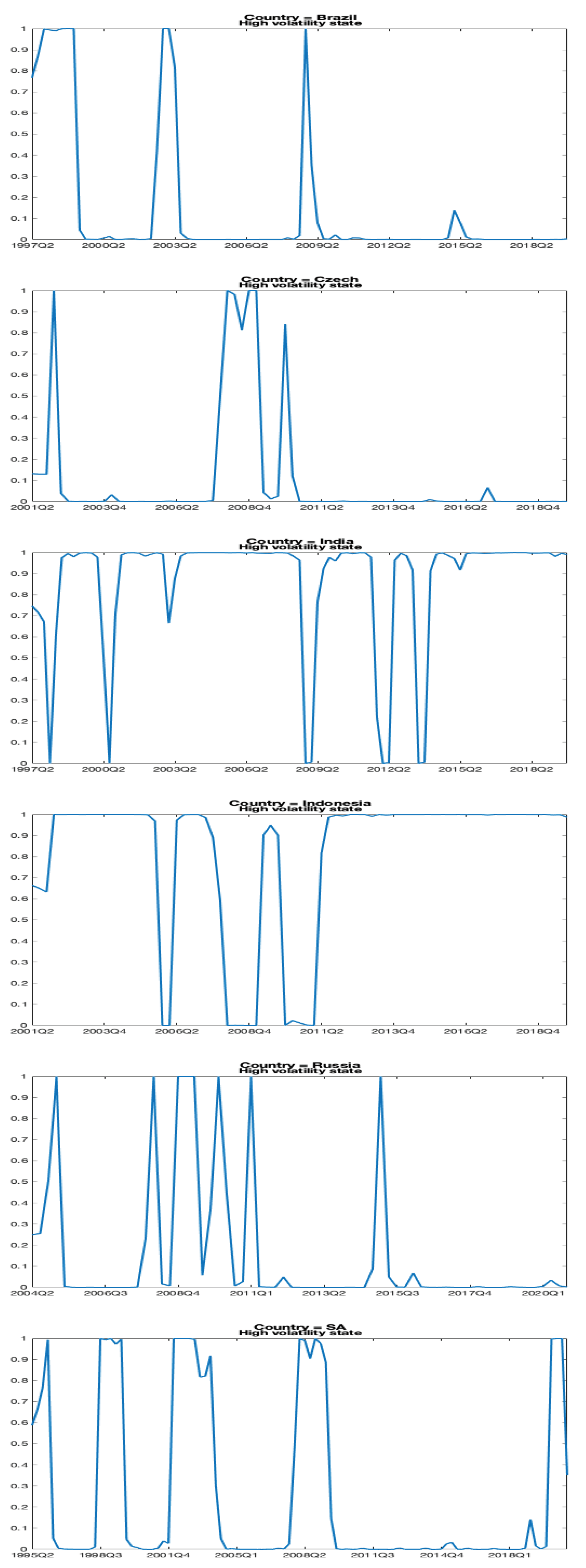
The volatilities of the structrual shocks have not remained constant too. They are larger in the high regime for all economies but India and Indonesia. Except for the latter economies, the probability of moving from the regime of high output volatility to the low one is larger than the opposite. Therefore, periods of high volatility, although recurrent, tend to be short-lived. We will come back to this when looking at the smoothed probabilities regimes. Russia has the largest terms of trade volatility in both low and high regimes. In the high regime, this volatility is more than double that of the other economies. Furthermore, in the low regime, the Russian volatility is still higher than the volatility of the remaining economies in both regimes. Moreover, within Russia, the terms of trade have the highest volatility after foreign output. This may be due to the fact that Russia is among the world’s top producers and exporters of oil and gas. Besides, the country has experienced multiple international economic sanctions that have disrupted its foreign trade. Russian inflation volatility is the second highest, in the high regime, after South Africa. A weaker response to exchange rate compared to the other economies may have hindered the ability to shelter the domestic economy from a volatile terms of trade, leading to a volatile inflation. India and South Africa are the next economies with a higher terms of trade volatility. For India, the high volatility occurs, instead, in the low output volatility regime. This regime coincides with a low response to both inflation and exchange rate in the policy rule, explaining the terms of trade volatility observed. The South African inflation volatility is the largest in the high regime. Athough the country has the second strongest exchange rate response in this regime, this period is short-lived (see Figure 1). Given its sizable terms of trade volatility relative to the other economies, a high inflation volatility is inevitable. The Czech Republic has the lowest estimated productivity, terms of trade and inflation volatility. At any point in time, the Czech central bank responds strongly to either inflation or exchange rate. These responses may lead to some price stability.

For the parameters that are regime invariant, only the productivity process seems less persistent for these economies. However, the terms of trade are more persistent than those obtained by Lubik and Schorfheide [3] and Alstadheim et al. [7] for developed economies. The measure of openness,

α

, indicates that the Czech Republic is the most opened economy, followed by Brazil. Interestingly, the former is the economy that responds the most to exchange rate deviation while the latter has the second strongest response in the low regime. As indicated by Lubik and Schorfheide [3], exchange rates have stronger domestic effect, the more opened the economy is, leading to an anti-inflationnary policy. The intertemporal elastiticy of substitution is similar to those obtained for small economies in the literature (See Lubik and Schorfheide [3] and Alstadheim et al. [7]).

There are two main findings. First, the terms of trade are among the top two volatile shocks. This supports the view that they are a significant source of business fluctuations for emerging economies as outlined by Uribe and Schmitt-Grohé [4]. Second, these economies attempt to smooth their respective exchange rates. The economies that respond strongly to exchange rate are therefore able to insulate themselves against volatile terms of trade. This, coupled with a robust response to inflation, reduces inflation volatility. Next, we look at the smooth probabilities for both policy parameters and structural shocks.

Figure 1 depicts the smoothed probabilities of being in the high regime,

S_{t}^{P o l} = H i g h

. This is the regime having a strong response to deviation of exchange rate from its target. The different economies have switched, at some point in the sample, between periods of low and high response. Brazil was in a low response regime from 1999 up to the end of 2006. Indeed, in 1999, Brazil abandoned the crawling peg and, consequently, adopted a flexible exchange rate regime in the month of January; and moved to the IT in July of the same year. From late 2006, the country moved to the high regime until 2017. This move coincides with the rise in foreign reserved starting form 2006 aimed at, according to Sandri [38], intervening in the foreign exchange market. The Czech Republic has been in the low regime for a brief period between 2007-2008. For most of the sample, despite the adoption of the IT framework in 1997, the country has responded strongly to exchange rate movements. Part of this period corresponds to the exchange rate commitment started by the country in 2015 with the aim of keeping the exchange rate against the Euro at or above a fixed rate [39]. India moved to a low regime in 1999. This year corresponds exactly to the period the exchange rate became market determined in the country, following the 1997-1998 East Asian crisis (see for example Tripathy [40]). The Indonesian economy has evolved, for most of the sample, between the two extreme regimes. From 2005, year of the adoption of the IT, the economy moved gradually to the low regime response. However, this move was short-lived. As stated earlier, the Bank of Indonesia monetary policy goals are price and exchange rate stability. It uses foreign exchange intervention to stabilize the domestic currency and control inflation. After evovling between the two regimes, Russia moved to the low regime in mid-2009. However, in 2014, year of the adoption of the IT framework, the country moved to the high regime. South Africa has evolved since the end of 1999, and for most of the sample, in the low regime. This period corresponds to the adoption of the IT framework by the South African Reserve Bank.

The smoothed probability for the high volatility regime,

S_{t}^{V o l} = H i g h

, is depicted in Figure 2. This is the regime with a high output volatility. It is worth noting that the other shocks may not neccessarily move in the same direction than output. This is the case for India and Indonesia, see Table 4. For the former economy, all the different shocks have a lower volatility when in the high regime while for the latter, only foreign output switches in the same direction than domestic output. The different economies have recorded a high output volatility during the period covering the 2007 Global finanical crisis. Moreover, the impact of the East Asian crisis of 1997-1998 is evident looking at the Indian Figure. For Brazil, the model captures well the heightened volatility during the crisis of 1997-1998 that led to the abandonment of the crawling peg. In addition, the deep recession that occured between 2015 and 2016 is also, to some extent, apparent in the figure. Russia has experienced several periods of high volatility due to the various international sanctions. We can also note the rise in volatility following the 2014-2015 Russian financial crisis due to a combination of various factors such as international sanctions, a sharp fall in oil prices with its consequences on the Russian currency [see [41]. The impact of the 2019 Coronavirus pandemic is visible in South Africa. The country went into a lockdown to contain the spread of the virus. In the second quarter of 2020, the South African GDP fell by 16.9%.10 In the next section, we discuss the impact of a terms of trade shock on these economies taking into account their responses to exchange rate.

5.3. Impulse response functions

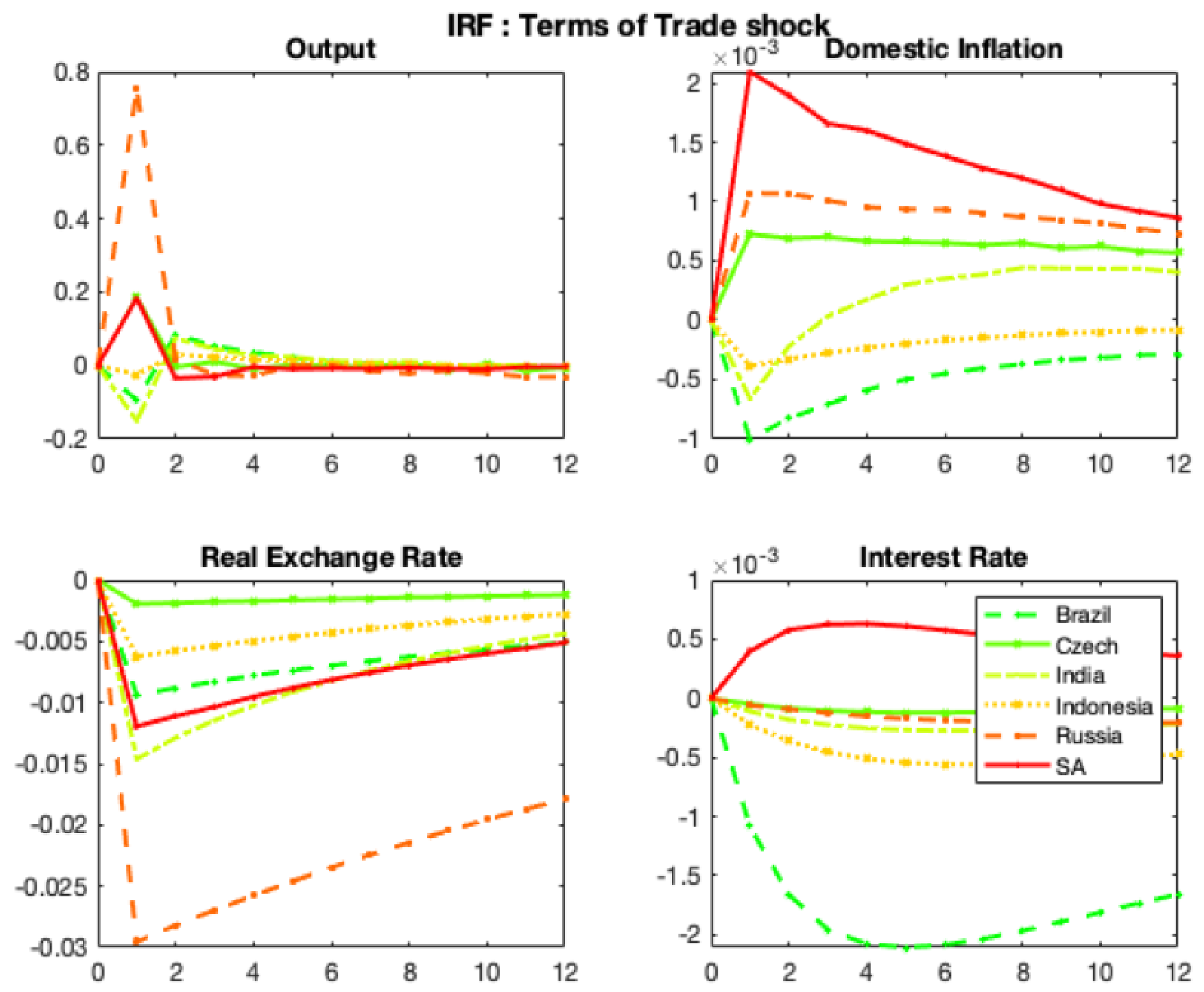
We examine whether the policy rule with a response to exchange rate deviation amplifies or reduces the effects of terms of trade on the different variables. We consider an improvement of the terms of trade stemming from an increase of export prices relative to import. We expect the respective domestic currencies to appreciate following this improvement. As highlighted by Alstadheim et al. [7], the impact on output and inflation depends on the exchange rate response. The currency will appreciate by much less if the economy is in a regime of high exchange rate response. This will reverse the initial exchange rate response and both output and inflation will increase.

Figure 3 depicts the generalized impulse response functions (IRFs) on output, exchange rate, domestic inflation and short tern interest rate for each economy. The improvement of the terms of trade leads to an appreciation of all the respective domestic currencies. Given that the Czech Republic has the strongest response to exchange rate in both low and high regimes, the domestic currency has recorded the least appreciation. This spurs both output and inflation. Russia has the lowest response to exchange rate, especially in the low regime. Therefore, the Russian currency appreciation is the most pronounced. However, despite this large appreciation, Russia has the largest output increase which spurred inflation. This rise may be explained by the strategic nature of Russian exports. Indeed, as explained earlier, Russia is among the top world’s producers and exporters of oil and gas. India has the second largest appreciation. Indeed, the country has spent a large part of the sample in a low regime with a very modest response to exchange rate. The strong appreciation leads to a fall of output and inflation. This is also the case for South Africa which has the second largest response to exchange rate in the high regime but spent the large part of the sample in the low regime with a moderate weight. However, despite the appreciation, both output and inflation rise. Brazil has the largest response, although not pronounced, in the low regime after the Czech Republic. The currency appreciation leads to a fall of output and inflation. Indonesia is the second economy with the least appreciation. Indeed, the country has evolved for the large part of the sample in a regime of strong response to exchange rate, leading to a less pronounced fall of output and inflation. The IRFs indicate a large fall of the Brazilian interest rate. Let us recall that the stylized facts, see Section 2, indicate that Brazil has the largest interest rate volatility. Moreover, from the estimation results, see Table 4, the policy rate has the highest volatility when Brazil responds strongly to exchange rate deviation.

The IRFs’ results indicate that the currency appreciation, following a terms of trade improvment, is dampened for economies that respond strongly to exchange rate movements. This leads to a rise in both output and inflation. However, for emerging economies that are large exporters of strategic commodities, a stronger appreciation does not hinder output growth. Next, we look at the variance decompositions of the different variables.

5.4. Variance decompositions

We assess the importance of the different shocks by computing the variance decompositions of our variables of interest. Table 5 reports the results. The Brazilian, Indian, Indonesian and South African outputs are mostly explained by world output innovations. However, for the Czech Republic, both world inflation and terms of trade are the most important drivers. For Russia, monetary policy and terms of trade contribute significantly to output volatility. Looking at the inflation rate, this variable is largely explained by world output in India and South Africa while in the remaining economies the different innovations do not play a significant role. The interest rate is mainly driven by terms of trade in Brazil, by world inflation in the Czech Republic, by world output in both India and South Africa; and by monetary policy and terms of trade in Indonesia. Interestingly, it is only in Russia that monetary policy innovations explain more than 80% of interest rates volatility. The role of the terms of trade in explaining domestic business cycles fluctuations can be seen by its large contribution into the respective exchange rates volatility. Indeed, the results indicate that more than 70% of the exchange rate volatility of the different economies, but South Africa, are explained by the terms of trade. Even for the latter economy, the contribution is a staggering 56%.

The results of the variance decompositions in general, and those of the terms of trade in particular, support the role played by foreign shocks in explaining business cycles fluctuations in emerging economies. According to Lubik and Schorfheide [3], a large terms of trade contribution into exchange rate volatility, as we find in this article, supports a response of central banks to exchange rate movements. Therefore, these emerging economies attempt to smooth exchange rate to insulate themselves against international price movements. The decompositions results are similar, among others, to those of Kose [5] and Lubik and Schorfheide [3] for small economies.

6. Conclusion

Do central banks respond to exchange rate movements? We answer this question for a sample of emerging economies that are commodities exporters and have adopted the IT as their monetary policy framework. These economies may be vulnerable to terms of trade movements as they export a limited number of commodities and have therefore an incentive to react to exchange rate movements. However, given their adopted monetary policy framework, they should not target any other variables besides inflation. In addition, we analyze the importance of the terms of trade in explaining their domestic business cycles fluctuations.

We estimate, separately for each economy, a regime switching open DSGE model using Bayesian techniques and quarterly data. We compare between a constant parameters and our regime switching model using the Laplace marginal data density after a posterior simulation. We find that the regime switching model fits the data better. The estimation results indicate that in certain periods, these emerging economies respond strongly to exchange rate movements while in others, some have a weaker response. We analyze the impact of a terms of trade improvement on different variables. We find that the different currencies appreciate following the shock. However, the stronger the response to exchange rate, the weaker the appreciation. The appreciation reversal leads to a rise in output and inflation for those economies that respond strongly to exchange rate and those who are major players in international trade such as Russia. Lastly, we use the variance decompositions to analyze the importance of the different innovations. We find that the terms of trade play a major role in explaining the business cycles fluctuations of these economies. Their large contribution into exchange rate volatility supports the finding that these economies respond to exchange rate movements.

In this article, we have identified the exchange rate stability as an additional monetary policy objective that can even supersede, for certain economies, the traditional goals. We have contrasted the impact of shocks on these economies that respond differently to exchange rate movements. We have identified the innovations that explain the business cycles of these economies. Thus, the regime switching framework has been able to better identify the regime changes in both policy and volatility of structural shocks for small open emerging economies that have different exposure to international trade.

Funding

This research received no external funding.

Data Availability Statement

This research has used secondary data publicly available. The different sources and transformations are indicated under the data section.

Acknowledgments

This research received administrative support from the Macroeconomics Research Unit of the School of Accounting, Economics and Finance of the University of KwaZulu-Natal, South Africa.

Conflicts of Interest

The author declares no conflicts of interest.

Abbreviations

The following abbreviations are used in this manuscript:

BRA	Brazil
CZE	Czech Republic
IND	India
INDO	Indonesia
RUS	Russia
SA	South Africa
I. Gamma	Inverse Gamma

1	The de jure is the announced exchange rate regime while the de facto is the actual regime implemented.
2	Our focus in this article is on research using structural models.
3	The emerging economies are those classified as emerging markets as per the FTSE Russel index. It distinguishes between developped, emerging (primary and secondary) and frontier markets. The economies used in this article fall under both primary and secondary emerging markets. They were selected based on data availability.
4	We split the sample into pre and post-IT adoption. The date of the adoption corresponds, for most, to a move to a flexible exchange rate regime. Due to lack of data pre-IT, we do not comment for the Czech Republic. However, a regime switching can still capture changes in policy and volatility even during the IT era.
5	The cutoff date is explained by the lack of recent data on terms of trade.
6	All the series, except the nominal effective exchange rates, are seasonally adjusted.
7	We have used the broad weights set as it provides the largest sample size for the economies under study.
8	Except for South Africa, the terms of trade for the remaining economies are only available in annual frequency.
9	Contrary to Alstadheim et al. [7] who use a tight prior for $α$ , the openness parameter, we allow a loose one given that open DSGE models literature for emerging economies is still at its infancy stage.
10	Author’s own calculations using the quartlery Real GDP of South Africa in domestic currency and seasonally adjusted from the Federal Reserve Bank of St Louis.

References

Levy-Yeyati, E.; Sturzenegger, F. Classifying exchange rate regimes: Deeds vs. words. European economic review 2005, 49, 1603–1635. [CrossRef]
Jahan, S. Inflation targeting: Holding the line. Finance & Development 2012, 4, 72–73.
Lubik, T.A.; Schorfheide, F. Do central banks respond to exchange rate movements? A structural investigation. Journal of Monetary Economics 2007, 54, 1069–1087. [CrossRef]
Uribe, M.; Schmitt-Grohé, S. Open economy macroeconomics; Princeton University Press, 2017.
Kose, M.A. Explaining business cycles in small open economies: ‘How much do world prices matter?’. Journal of International Economics 2002, 56, 299–327.
Dong, W. Do central banks respond to exchange rate movements? Some new evidence from structural estimation. Canadian Journal of Economics/Revue canadienne d’économique 2013, 46, 555–586. [CrossRef]
Alstadheim, R.; Bjørnland, H.C.; Maih, J. Do central banks respond to exchange rate movements? A markov-switching structural investigation of commodity exporters and importers. Energy Economics 2021, 96, 105138. [CrossRef]
Mohanty, M.S.; Klau, M. Monetary policy rules in emerging market economies: Issues and evidence. In Monetary policy and macroeconomic stabilization in Latin America; Springer, 2005; pp. 205–245.
Ortiz, A.; Sturzenegger, F. Estimating SARB’s policy reaction rule. South African Journal of Economics 2007, 75, 659–680.
Alpanda, S.; Kotzé, K.; Woglom, G. The role of the exchange rate in a New Keynesian DSGE model for the South African economy. South African Journal of Economics 2010, 78, 170–191. [CrossRef]
Lubik, T.A.; Schorfheide, F. Testing for indeterminacy: An application to US monetary policy. American Economic Review 2004, 94, 190–217. [CrossRef]
Gali, J.; Monacelli, T. Monetary policy and exchange rate volatility in a small open economy. The Review of Economic Studies 2005, 72, 707–734. [CrossRef]
Grivoyannis, E. The New Brazilian Economy; Springer, 2017.
Da Fonseca, M.A. Brazil’s Real plan. Journal of Latin American Studies 1998, 30, 619–639.
Clements, B. Development focus: The Real plan, poverty and income distribution in Brazil. Finance & Development 1997, 34.
Afonso, J.R.; Araújo, E.C.; Fajardo, B.G. The role of fiscal and monetary policies in the Brazilian economy: Understanding recent institutional reforms and economic changes. The Quarterly Review of Economics and Finance 2016, 62, 41–55. [CrossRef]
Coats, W.L.; Laxton, D.; Rose, D. The Czech National Bank’s Forecasting and Policy Analysis System; Czech National Bank, 2003.
Mohan, R.; Patra, M. Monetary policy transmission in India. In Monetary policy frameworks for emerging markets; Edward Elgar Publishing, 2009.
Balakrishnan, P.; Parameswaran, M. What lowered inflation in India: Monetary policy or commodity prices? Indian Economic Review 2022, 57, 97–111.
Dua, P. Monetary policy framework in India. Indian Economic Review 2020, 55, 117–154. [CrossRef]
McLeod, R.H. Towards improved monetary policy in Indonesia. Bulletin of Indonesian Economic Studies 2003, 39, 303–324. [CrossRef]
Ramayandi, A.; Rosario, A. Monetary policy discipline and macroeconomic performance: The case of Indonesia. Asian Development Bank Economics Working Paper Series 2010.
Chowdhury, A.; Siregar, H. Indonesia’s monetary policy dilemma: Constraints of inflation targeting. The Journal of Developing Areas 2004, pp. 137–153. [CrossRef]
Ahokpossi, M.C.; Isnawangsih, A.; Naoaj, M.S.; Yan, T. The Impact of Monetary Policy Communication in an Emerging Economy: The Case of Indonesia; International Monetary Fund, 2020.
Granville, B.; Mallick, S. Monetary Policy in Russia. In Return to Growth in CIS Countries; Springer, 2006; pp. 73–89.
Hanson, P. Russian Economic Policy and the Russian Economic System: Stability versus Growth 2019.
Kumo, W.L. Inflation Targeting Monetary Policy, Inflation Volatility and Economic Growth in South Africa. Technical report, African Development Bank, 2015.
Mandeya, S.M.T.; Ho, S.Y. Inflation, inflation uncertainty and the economic growth nexus: An impact study of South Africa. MethodsX 2021, 8, 101501. [CrossRef]
Bonga-Bonga, L. Assessing the effectiveness of the monetary policy instrument during the inflation targeting period in South Africa. International Journal of Economics and Financial Issues 2017, 7, 706–713.
Fraga, A.; Goldfajn, I.; Minella, A. Inflation targeting in emerging market economies. NBER macroeconomics annual 2003, 18, 365–400. [CrossRef]
Holland, M. Exchange rate volatility and the fear of floating in Brazil. Revista EconomiA 2006.
Maih, J. Efficient Perturbation Methods for Solving Regime-Switching DSGE Models. Technical report, working paper 2015/1, Norges Bank, 2015.
Kim, C.J.; Nelson, C.R. Has the US economy become more stable? A Bayesian approach based on a Markov-switching model of the business cycle. Review of Economics and Statistics 1999, 81, 608–616. [CrossRef]
Karaboga, D.; others. An idea based on honey bee swarm for numerical optimization. Technical report, Technical report-tr06, Erciyes university, engineering faculty, computer …, 2005.
Karaboga, D.; Akay, B. A comparative study of artificial bee colony algorithm. Applied mathematics and computation 2009, 214, 108–132. [CrossRef]
Liu, Z.; Waggoner, D.F.; Zha, T. Sources of macroeconomic fluctuations: A regime-switching DSGE approach. Quantitative Economics 2011, 2, 251–301. [CrossRef]
Debortoli, D.; Maih, J.; Nunes, R. Loose commitment in medium-scale macroeconomic models: Theory and applications. Macroeconomic Dynamics 2014, 18, 175–198. [CrossRef]
Sandri, D. FX intervention to stabilize or manipulate the exchange rate? Inference from profitability. Journal of International Money and Finance 2023, 131, 102786. [CrossRef]
Hajkova, D. Monetary Policy and Exchange Rate Commitment in the Czech Republic. In Negative Euro Area Interest Rates and Spillovers on Western Balkan Central Bank Policies and Instruments; International Monetary Fund, 2017.
Tripathy, R. Intervention in foreign exchange markets: The approach of the Reserve Bank of India. BIS Papers 2013, 73.
Viktorov, I.; Abramov, A. The 2014-15 financial crisis in Russia and the foundations of weak monetary power autonomy in the international political economy. New political economy 2020, 25, 487–510. [CrossRef]

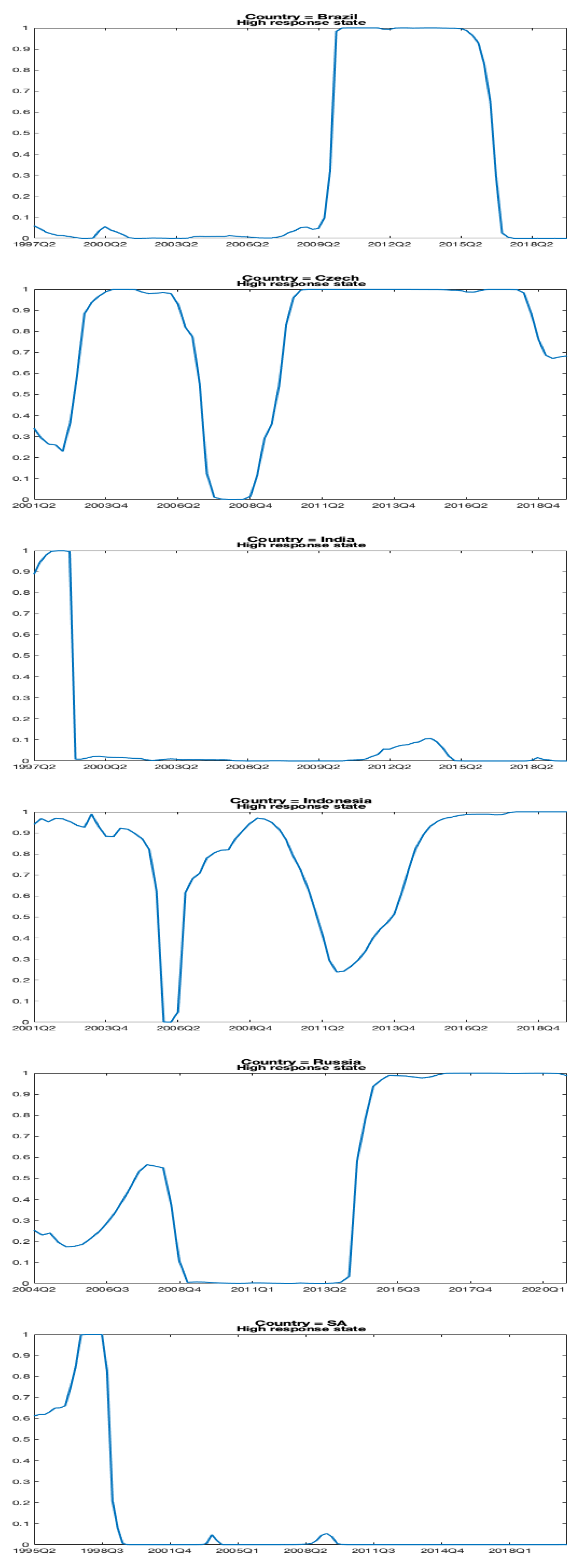
Figure 1. Smoothed Probabilities of High Response -

S_{t}^{P o l} = H i g h

Figure 1. Smoothed Probabilities of High Response -

S_{t}^{P o l} = H i g h

Figure 2. Smoothed Probabilities of High Volatility -

S_{t}^{V o l} = H i g h

Figure 2. Smoothed Probabilities of High Volatility -

S_{t}^{V o l} = H i g h

Figure 3. Generalized IRFs of a Terms of Trade Shock

Table 1. Measurement variables volatility

	BRA	CZE	IND	INDO	RUS	SA
GDP	1.61/8.78	5.12	3.61/1.98	1.05/12.46	7.25/8.37	5.28/6.80
Inflation	5.48/3.29	2.11	3.87/3.55	3.74/5.04	3.42/5.05	3.77/3.31
Interest rate	4.08/5.39	1.50	0.61/0.73	0.69/3.07	3.01/2.99	2.24/1.97
Exchange rate	0.02/0.07	0.02	0.03/0.02	0.04/0.04	0.04/0.07	0.04/0.05
Terms of trade	1.36/1.85	0.52	0.85/1.71	2.23/1.30	6.05/5.28	5.65/2.73

Note: Standard deviation prior IT to the left and post IT to the right. The variables are in log deviation of their means.

Table 2. Priors and posterior modes - Constant parameters model

Parameters	Prob. Dist	Low	High	BRA	CZE	IND	INDO	RUS	SA
$ρ_{i}$	Beta	0.500	0.950	0.855	0.940	0.949	0.799	0.941	0.924
$γ_{π}$	I. Gamma	0.800	3.000	1.780	1.183	1.146	2.008	1.137	1.455
$γ_{y}$	I. Gamma	0.005	3.000	0.490	0.023	0.985	0.005	1.874	0.516
$γ_{e}$	I. Gamma	0.005	3.000	1.435	3.000	0.101	0.092	1.830	0.005
$σ_{i}$	I. Gamma	1.e-05	10.00	0.007	0.001	0.001	0.001	0.014	0.002
$σ_{y}$	I. Gamma	0.005	15.00	0.012	0.005	0.005	0.008	0.005	0.006
$σ_{π}$	I. Gamma	1.e-05	10.00	0.002	0.001	0.006	0.005	0.006	0.005
$σ_{z}$	I. Gamma	1.e-05	10.00	0.008	0.001	0.014	0.004	0.021	0.014
$σ_{q}$	I. Gamma	1.e-05	10.00	0.011	0.004	0.015	0.007	0.036	0.017

Table 3. Model comparison

Model	BRA	CZE	IND	INDO	RUS	SA
Constant	-1450.1	-833.4	-1442.3	-1176.6	-1266.5	-1662.4
Switching	-1409.3	-816.5	-1342.2	-1131.0	-1126.2	-1528.0

Table 4. Priors and posterior modes - Regime switching model

Parameters	Prob. Dist.	Low	High	BRA	CZE	IND	INDO	RUS	SA
$τ$	Beta	0.010	0.999	0.074	0.858	0.192	0.201	0.881	0.495
$κ$	Gamma	0.010	10.00	0.024	0.030	0.054	0.010	0.010	0.084
$α$	Beta	0.010	0.999	0.217	0.224	0.118	0.117	0.038	0.066
$ρ_{q}$	Beta	0.010	0.999	0.951	0.964	0.907	0.932	0.956	0.925
$ρ_{y *}$	Beta	0.010	0.999	0.611	0.895	0.986	0.545	0.986	0.992
$ρ_{π^{*}}$	Beta	0.010	0.999	0.580	0.986	0.875	0.480	0.552	0.498
$ρ_{z}$	Beta	0.010	0.999	0.591	0.500	0.319	0.512	0.491	0.186
coef_tp_L_H	Beta	0.010	0.500	0.017	0.055	0.010	0.024	0.037	0.011
coef_tp_H_L	Beta	0.010	0.500	0.041	0.010	0.061	0.062	0.028	0.018
$ρ_{i} (S_{t}^{P o l}, L)$	Beta	0.500	0.950	0.624	0.813	0.950	0.860	0.922	0.908
$ρ_{i} (S_{t}^{P o l}, H)$	Beta	0.500	0.950	0.878	0.932	0.935	0.747	0.891	0.761
$γ_{π} (S_{t}^{P o l}, L)$	I. Gamma	0.800	3.000	1.512	1.438	0.993	1.511	1.284	1.365
$γ_{π} (S_{t}^{P o l}, H)$	I. Gamma	0.800	3.000	1.339	0.982	1.658	1.351	1.613	1.403
$γ_{y} (S_{t}^{P o l}, L)$	I. Gamma	0.005	3.000	0.124	0.146	0.085	0.056	0.136	0.398
$γ_{y} (S_{t}^{P o l}, H)$	I. Gamma	0.005	3.000	0.027	0.395	0.395	0.503	0.390	0.853
$γ_{e} (S_{t}^{P o l}, L)$	I. Gamma	0.005	3.000	0.184	0.205	0.074	0.048	0.036	0.106
$γ_{e} (S_{t}^{P o l}, H)$	I. Gamma	0.005	3.000	0.263	1.930	0.611	0.467	0.352	0.731
vol_tp_L_H	Beta	0.001	0.500	0.027	0.019	0.244	0.120	0.080	0.053
vol_tp_H_L	Beta	0.010	0.500	0.125	0.159	0.053	0.043	0.257	0.138
$σ_{i} (S_{t}^{V o l}, L)$	I. Gamma	1.e-05	10.00	0.002	0.001	0.003	0.003	0.002	0.001
$σ_{i} (S_{t}^{V o l}, H)$	I. Gamma	1.e-05	20.00	0.011	0.002	0.001	0.002	0.011	0.002
$σ_{y} (S_{t}^{V o l}, L)$	I. Gamma	0.005	15.00	0.005	0.005	0.005	0.007	0.006	0.005
$σ_{y} (S_{t}^{V o l}, H)$	I. Gamma	0.005	20.00	0.007	0.008	0.005	0.008	0.007	0.007
$σ_{π} (S_{t}^{V o l}, L)$	I. Gamma	1.e-05	10.00	0.004	0.001	0.026	0.017	0.006	0.003
$σ_{π} (S_{t}^{V o l}, H)$	I. Gamma	1.e-05	20.00	0.017	0.009	0.012	0.002	0.021	0.024
$σ_{z} (S_{t}^{V o l}, L)$	I. Gamma	1.e-05	10.00	0.007	0.001	0.026	0.013	0.014	0.013
$σ_{z} (S_{t}^{V o l}, H)$	I. Gamma	1.e-05	20.00	0.010	0.007	0.012	0.003	0.054	0.021
$σ_{q} (S_{t}^{V o l}, L)$	I. Gamma	1.e-05	10.00	0.010	0.003	0.020	0.016	0.022	0.013
$σ_{q} (S_{t}^{V o l}, H)$	I. Gamma	1.e-05	20.00	0.012	0.008	0.015	0.003	0.059	0.020
$σ_{y^{*}} (S_{t}^{V o l}, L)$	I. Gamma	1.e-05	15.00	0.004	0.031	0.008	0.008	0.037	0.014
$σ_{y^{*}} (S_{t}^{V o l}, H)$	I. Gamma	1.e-05	20.00	0.037	0.125	0.003	0.034	0.164	0.099
$σ_{π^{*}} (S_{t}^{V o l}, L)$	I. Gamma	1.e-05	15.00	0.003	0.001	0.006	0.005	0.003	0.002
$σ_{π^{*}} (S_{t}^{V o l}, H)$	I. Gamma	1.e-05	20.00	0.008	0.005	0.003	0.002	0.005	0.004
stderr y	I. Gamma	1.e-05	20.00	5.347	5.286	2.462	10.00	7.556	7.487
stderr $π$	I. Gamma	1.e-05	20.00	1.366	1.331	3.408	2.853	0.007	0.035
stderr $y^{*}$	I. Gamma	1.e-05	20.00	3.463	0.006	3.013	4.887	0.007	2.132
stderr $π^{*}$	I. Gamma	1.e-05	20.00	0.007	0.705	0.007	0.007	0.007	0.007

Note: L=Low regime; H=High regime; tp=transition probability.

Table 5. Variance decompositions

Shocks	Policy	Terms of Trade	Technology	World output	World inflation
BRAZIL
Output	1.443	1.205	3.052	92.598	0.029
Inflation	3.605	6.998	2.465	3.415	0.094
Interest rate	15.419	63.859	2.708	5.560	0.115
Exchange rate	0.184	92.662	0.126	0.174	2.606
CZECH
Output	18.039	30.969	0.783	4.289	38.991
Inflation	1.558	13.436	0.007	0.266	83.378
Interest rate	2.717	0.772	0.013	0.027	96.360
Exchange rate	2.094	71.774	0.010	0.358	23.943
INDIA
Output	11.272	1.209	8.775	73.292	0.215
Inflation	24.451	2.913	1.421	60.680	0.750
Interest rate	6.611	3.644	0.216	89.117	0.064
Exchange rate	1.661	89.751	0.097	4.122	3.704
INDONESIA
Output	3.272	1.130	4.993	81.085	0.029
Inflation	1.078	1.739	0.213	0.854	0.009
Interest rate	29.985	24.167	2.366	17.711	0.217
Exchange rate	0.101	87.487	0.020	0.080	3.307
RUSSIA
Output	44.237	32.203	16.346	0.275	0.044
Inflation	2.726	12.191	0.107	0.606	0.003
Interest rate	82.073	0.684	4.658	1.182	0.051
Exchange rate	0.034	98.757	0.001	0.007	0.162
SA
Output	0.788	0.425	0.518	94.648	0.028
Inflation	0.244	1.988	0.023	90.882	0.010
Interest rate	0.199	1.175	0.032	97.874	0.005
Exchange rate	0.107	56.414	0.010	39.923	0.534

Disclaimer/Publisher’s Note: The statements, opinions and data contained in all publications are solely those of the individual author(s) and contributor(s) and not of MDPI and/or the editor(s). MDPI and/or the editor(s) disclaim responsibility for any injury to people or property resulting from any ideas, methods, instructions or products referred to in the content.

© 2024 by the authors. Licensee MDPI, Basel, Switzerland. This article is an open access article distributed under the terms and conditions of the Creative Commons Attribution (CC BY) license (http://creativecommons.org/licenses/by/4.0/).

Copyright: This open access article is published under a Creative Commons CC BY 4.0 license, which permit the free download, distribution, and reuse, provided that the author and preprint are cited in any reuse.

MDPI Initiatives

Important Links

Choose an area of interest and we will send you notifications of new preprints at your preferred frequency.

Disclaimer

Do Central Banks Respond to Exchange Rate Movements? A Structural Analysis of Selected Inflation Targeters Emerging Economies

Abstract

1. Introduction

2. Some stylized facts

3. A regime switching DSGE model

3.1. The model

3.2. The Markov switching rational expectation framework

4. Data and Bayesian estimation

4.1. Data

4.2. Priors and estimation

5. Results

5.1. Time invariant rational expectations

5.2. Regime switching rational expectations

5.3. Impulse response functions

5.4. Variance decompositions

6. Conclusion

Funding

Data Availability Statement

Acknowledgments

Conflicts of Interest

Abbreviations

References

MDPI Initiatives

Important Links

Subscribe