Preprint

Article

Optimal Battery Energy Storage Dispatch for the Day-Ahead Electricity Market

Altmetrics

Downloads

116

Views

Comments

A peer-reviewed article of this preprint also exists.

Julio Gonzalez-Saenz,

Victor Becerra^*

Julio Gonzalez-Saenz,

Victor Becerra^*

This version is not peer-reviewed

Submitted:

22 March 2024

Posted:

25 March 2024

You are already at the latest version

Alerts

Abstract

This work presents an innovative application of optimal control theory to the strategic scheduling of battery storage in the day-ahead electricity market, with a focus on enhancing profitability while factoring in battery degradation. The study incorporates in the optimisation framework the cost of battery capacity degradation, the effects of capacity degradation and internal resistance degradation into dynamics. We employ a continuous-time representation of the dynamics, in contrast with many other studies that use a discrete-time approximation with rather coarse intervals. We adopt an equivalent circuit model coupled with empirical degradation parameters to simulate a battery cell’s behaviour and degradation mechanisms with good support from experimental data. Utilising direct collocation methods with mesh refinement allows for precise numerical solutions to the complex, nonlinear dynamics involved. Through a detailed case study of Belgium’s day-ahead electricity market, we determine the optimal charging and discharging schedules under varying objectives: maximizing net revenues, profits considering capacity degradation, and profits considering both capacity degradation and internal resistance increase due to degradation. The results demonstrate the viability of our approach and underscore the significance of integrating degradation costs into the market strategy for battery operators, alongside its effects on the battery’s dynamic behaviour. Our methodology extends previous work by offering a more comprehensive model that empirically captures the intricacies of battery degradation, including a fine and adaptive time domain representation, focusing on the day-ahead market, and utilising accurate direct methods for optimal control. The paper concludes with insights into the potential of optimal control applications in energy markets and suggestions for future research avenues.

Keywords:

Subject: Engineering - Electrical and Electronic Engineering

1. Introduction

According to the latest prediction of the European Commission, the percentage of electricity generated from renewable sources such as solar and wind will increase from 37% in 2020 to over 60% by 2030 [1]. In March 2023, the European Commission proposed a reform of the electricity market in the EU as part of its ambitious goal [2]. This reform aims at providing more resiflience to the market. It enhances the protection of the consumers by using more long-term contracts, such as power purchase agreements, improving the energy pricing policies and support of investment, and encouraging economic growth.

Electricity prices in a deregulated power system, such as the European, are determined by market players who consider the supply and demand of electricity. The most common market type is the day-ahead market, where electricity trading involves buying and selling electricity the day before the actual production and delivery [3]. The price structure of all market transactions is established through the analysis of all supply and demand bids. A power producer looking to enter the day-ahead electricity market aims to maximise their profits while ensuring reliable delivery of electricity, something they strive to achieve by optimising their production schedule and pricing strategy to sell electricity at the highest possible price while managing their operational costs and adhering to regulatory requirements and grid reliability standards. Various models and algorithms have been proposed to analyse bidding strategies in the literature. Traditionally, these approaches can be categorised into four main groups: optimisation models, game theory-based models, agent-based models, and hybrid models [4].

Battery storage plays an increasingly important in the day-ahead electricity market by leveraging its unique attributes—such as flexibility, fast response, and the ability to capitalize on price differentials—to enhance the operator’s market position, support grid stability, and contribute to the transition towards a more sustainable energy system. Their profitability lies in strategically purchasing energy during periods of low prices and storing it in the battery, subsequently capitalising on higher market prices by selling the stored energy and discharging the battery. The battery degradation cost at each charge/discharge cycle is often overlooked or not adequately addressed while designing the control policy for the battery’s participation in the market. Since this degradation cost is hard to assess and varies greatly depending on operational conditions, battery models usually rely on an empirical approach based on fitting measured degradation curves. These models have the advantages of being relatively simple and computationally inexpensive.

Optimal control is a mathematical theory that seeks to optimise a performance index associated with a dynamical system by choosing the time-domain profiles of independent variables called the control inputs. The theory and methods of optimal control have found application in a variety of areas ranging from aerospace, robotics, and process control, to the management of commodity markets. Generally speaking, a generic optimal control formulation with battery degradation constraints can be utilised to mathematically describe the battery’s profitable participation in the day-ahead electricity market. Remarkably, this approach has been relatively underutilised in existing studies despite its potential usefulness. One such study is presented in reference [5], which formulated the optimal control problem with an unconventional definition of battery degradation to examine energy dispatch in a wind farm. In contrast, the author of reference [6] formulated three optimal control problems to investigate the optimisation of profits in the day-ahead market. The author factored in the effect of battery degradation in the objective functional, which is considered in the optimisation process. Another approach is presented in reference [7], where the authors accounted for battery degradation by defining the state of health as an additional state variable and then considering it in the objective function.

Formulating the optimal energy dispatch accurately considering battery degradation is challenging and requires a well-designed modelling framework with a deep understanding of the battery’s chemistry. A vast amount of literature discusses the different types of battery models and their associated degradation phenomena. However, the majority of battery degradation studies are based on holistic approaches and involve results derived from laboratory experiments.

Numerical methods are indispensable to obtain a solution for models characterised by complex, nonlinear differential equations, such as the one proposed in this work. Specific computational methodologies exist, such as direct collocation methods, that help numerically solve the underlying optimal control problem.

Several authors [8,9,10,11,12] optimise the dispatch strategy of battery energy storage systems in day-ahead electricity markets using highly simplified discrete-time models of the battery storage systems, and relatively coarse time intervals between 15 minutes to one hour.

This study employs an optimal control methodology to address the problem of scheduling battery charging and discharging for the day-ahead electricity market. We focus on a case study aimed at maximising the profit from a battery’s participation in Belgium’s day-ahead electricity market. We used an equivalent circuit model to represent a battery cell, along with an empirical degradation model to consider the reduction of capacity and the increase in internal resistance resulting from degradation mechanisms. The work presented here extends the model, methods and results given in [6], through the use of direct collocation methods with mesh refinement, the incorporation of the effects of degradation in the internal resistance, and considering capacity degradation in the model state equations.

Section 2 of this paper provides a review of the literature concerning battery models and numerical techniques employed to solve optimal control problems. Section 3 familiarises the reader with the day-ahead electricity price and formulates two different optimal control problems. Section 4 presents the solutions to the problems using direct collocation techniques. The paper concludes with section 5, which offers final remarks and discusses future work.

2. Literature Review

The study of profit maximisation when energy storage providers participate in the day-ahead electricity market is a growing research area. Recent work [13] focused on a self-scheduling and re-dispatching optimisation problem. The formulation considers battery degradation and combines stochastic and mixed integer-linear programming. However, the method is computationally expensive. Furthermore, other researchers have studied the same problem using a simplified approach to mixed integer-linear programming, such as [14] and [15]. However, they often neglect or oversimplify the costs associated with battery degradation.

Similarly, reference [12] investigated the optimal day-ahead pricing policy with for a lead-acid battery employing a degradation model based on a cubic polynomial. While the vector of decision variables minimised the objective function for the day ahead, the solution did not consider the system dynamics.

Only a few researchers have viewed energy dispatch as an optimal control problem. For instance, [16] utilised model predictive control to optimise the operation of a lead-acid battery and minimise the output power deviations from the predefined agreement. Additionally, the control method examined by the author proposed a heuristic technique to prolong the battery’s lifespan rather than relying on degradation models. The technique reduces degradation by adding inequality constraints to the state of charge. In that manner, deep discharge and high values of the state of charge are avoided, increasing the battery life but limiting the use of the battery’s full capacity. While the technique heuristically reduces degradation, the dynamics of the charge/discharge cycle are not considered.

In a recent conference paper [17], the authors presented a degradation model for lead-acid batteries considering corrosion and mass degradation. The degradation model is succinctly described but applies mainly to lead chemical species. A degradation model developed for lead chemical species may not accurately capture the degradation processes and dynamics in lithium-ion systems.

2.1. Battery Models

Mathematical modelling is very useful for the study of a battery’ behaviour and the optimisation of its operation when participating in the electricity market. While experimental testing is beneficial, it can be expensive and time consuming. The mathematical model of a real-world battery is often dynamic, complex, distributed, and nonlinear, although some simplifications are possible.

In [6], the author delved into modelling and formulating an optimal control of lithium-ion batteries for the day-ahead energy market. Different profiles were suggested for optimising the battery energy storage system operation, considering the price of electricity in Belgium’s day-ahead electricity market. The proposed algorithm performs the necessary calculations to decide when to charge or discharge the battery and at what rate. Three different battery models were used to assess the effect of degradation: the bucket model, an empirical battery model, and a capacity reduction model.

An effective technique for simulating batteries is the holistic approach, which views the battery as a single entity rather than a collection of separated parts. The equivalent circuit model is an example of an empirical holistic model, where the model’s parameters and components, such as battery capacity, capacitance and resistance, along with the open circuit voltage function, are usually estimated by fitting the model predictions to experimental data. The simplicity of the model structure makes the equivalent circuit model easily accessible and widely used in various applications. With minimal computational complexity, this type of model provide valuable insights and predictions. Additionally, these models rely on historical data and empirical observations to validate and improve their predictions. By comparing the model output with real-world data, they can be fine-tuned and re-calibrated for increased accuracy and reliability.

The empirical holistic battery model has been successfully used in battery simulation frameworks, as demonstrated in the work described in [18], which does not consider battery degradation. In [19], the authors also took a holistic approach to finding the best automotive battery. While acknowledging that previous studies have shown the effects of electrothermal load and time on battery ageing, their study did not address degradation in the problem formulation. In contrast, [20] created a comprehensive model for a specific battery that considers both cycling degradation and calendar ageing. While the model is limited to a specific chemistry, its application can be extended to numerous other applications.

2.2. Capacity Reduction Modelling

2.2.1. Cycling Ageing

Several studies predict a linear dependency between the reduction in battery capacity and the number of charge/discharge cycles to which it is subjected [21]. However, in [22,23,24], the data showed that for all the charging/discharging current used during the cycle ageing testing, the model equations favoured a power law relationship pivoting very close to an exponent of value 0.5. The author of [23] argued that the dependency of time on the square root is a better representation of ageing mechanisms that involve diffusion and parasitic reactions than a linear dependency. Thus, it is generally accepted that Equation (1) establishes the relation between the capacity reduction during battery cycling,

C_{c y l}

, and the charge passing through the battery:

\begin{matrix} C_{c y l} = 1 - β_{c a p} \cdot \sqrt{Q} \end{matrix}

(1)

where

β_{c a p}

is the cycling ageing factor for capacity reduction and Q is the charge.

On the other hand, it is widely accepted that the increase in the internal battery resistance is the primary factor contributing to the capacity loss of lithium-ion batteries [25]. In line with previous studies, the authors of [26] reported that all the cells tested demonstrated a robust linear degradation behaviour, independently of the testing conditions, with slightly more rapid fade at the beginning of the cycling. Moreover, in reference [27], the authors used a simple and relatively intuitive model to analyse the coupled effect of resistance growth and cycling ageing. They concluded that a linear model fitted the curve satisfactorily. Hence, it is generally accepted that Equation (2) represents the relation between the resistance increase during battery cycling,

R_{c y l}

, and the charge passing through the battery:

R_{c y l} = 1 + β_{r e s} \cdot Q

(2)

where

β_{r e s}

is the cycling ageing factor for resistance increase.

2.2.2. Calendar Ageing

Calendar ageing is the natural deterioration of a lithium battery that occurs over time, regardless of usage. When the battery remains inactive, parasitic reactions in the anode material occur between the electrolyte and the electrode, resulting in lithium-ion loss and the creation of a solid-electrolyte interphase layer [28]. This thin film layer can raise the battery’s internal resistance and decrease the battery capacity. Moreover, repeated charge and discharge cycles can intensify calendar ageing even at low levels.

In reference [20], the authors normalised the battery capacity, C, to apply a degradation factor based on calendar ageing. Moreover, it is indicated that the capacity varies with time, particularly with

t^{0.75}

, according to the following relationship:

C_{a g e} = 1 - α_{c a p} t^{0.75}

(3)

where

α_{a g e}

corresponds to the ageing factor to be determined using curve fitting techniques and t is the simulation time in days.

Similarly, as per the references cited in the literature [24,29], it is widely accepted that the primary reason behind the ageing of carbon-based anode materials is the formation of a solid electrolyte interphase. This thin film is created when the electrolyte breaks down and consumes lithium, leading to an increase in resistance. Following the model presented in reference [20], the increase in the resistance is a function of

t^{0.75}

and according to the following relationship:

R_{a g e} = 1 + α_{r e s} t^{0.75}

(4)

The total degradation in the capacity and in the internal resistance due to calendar ageing and cycling is given in Equation (5):

\begin{matrix} C_{d e g} & = 1 - α_{c a p} \cdot t^{0.75} - β_{c a p} \cdot \sqrt{Q} \\ R_{d e g} & = 1 + α_{r e s} \cdot t^{0.75} + β_{r e s} \cdot Q \end{matrix}

(5)

where

α_{r e s}

and

α_{c a p}

are functions of the mean voltage,

V_{m e a n}

, and ambient temperature,

T_{a}

, and

β_{r e s}

and

β_{c a p}

are functions of the the root-mean square voltage,

V_{r m s}

, and the depth of discharge,

D_{o d}

Furthermore,

D_{o d} = 1 - S_{o C}

, where

S_{o C}

represents the state of charge of the battery.

3. Problem Statement

Electricity buyers and sellers in the real world are keenly interested in maximising their profits in the day-ahead electricity market, which spans 24 hours and publishes prices a day before actual buying and selling. In order to comply with the energy trading market rules, the operator who sells energy should commit to selling a certain amount of electricity. These rules greatly depend on the country or the region where they apply, but essentially, the core rules that regulate market participants are remarkably alike.

This study uses an optimal control methodology to determine the most effective charge/discharge energy dispatch strategy for a lithium-ion battery energy storage system in the day-ahead electricity market. Direct collocation with automatic mesh refinement methods is employed to compare the optimal solutions of two battery models. This approach differs from the previous study reported in [30], which compared the optimal control trajectories resulting from the use of three different battery models without describing how the optimal control problems were solved. Our goal is to identify the battery’s operational profile that maximises profit, measured as the difference between net revenue (considering the sale and purchase of electricity while discharging and charging the battery, respectively), and the cost of battery degradation.

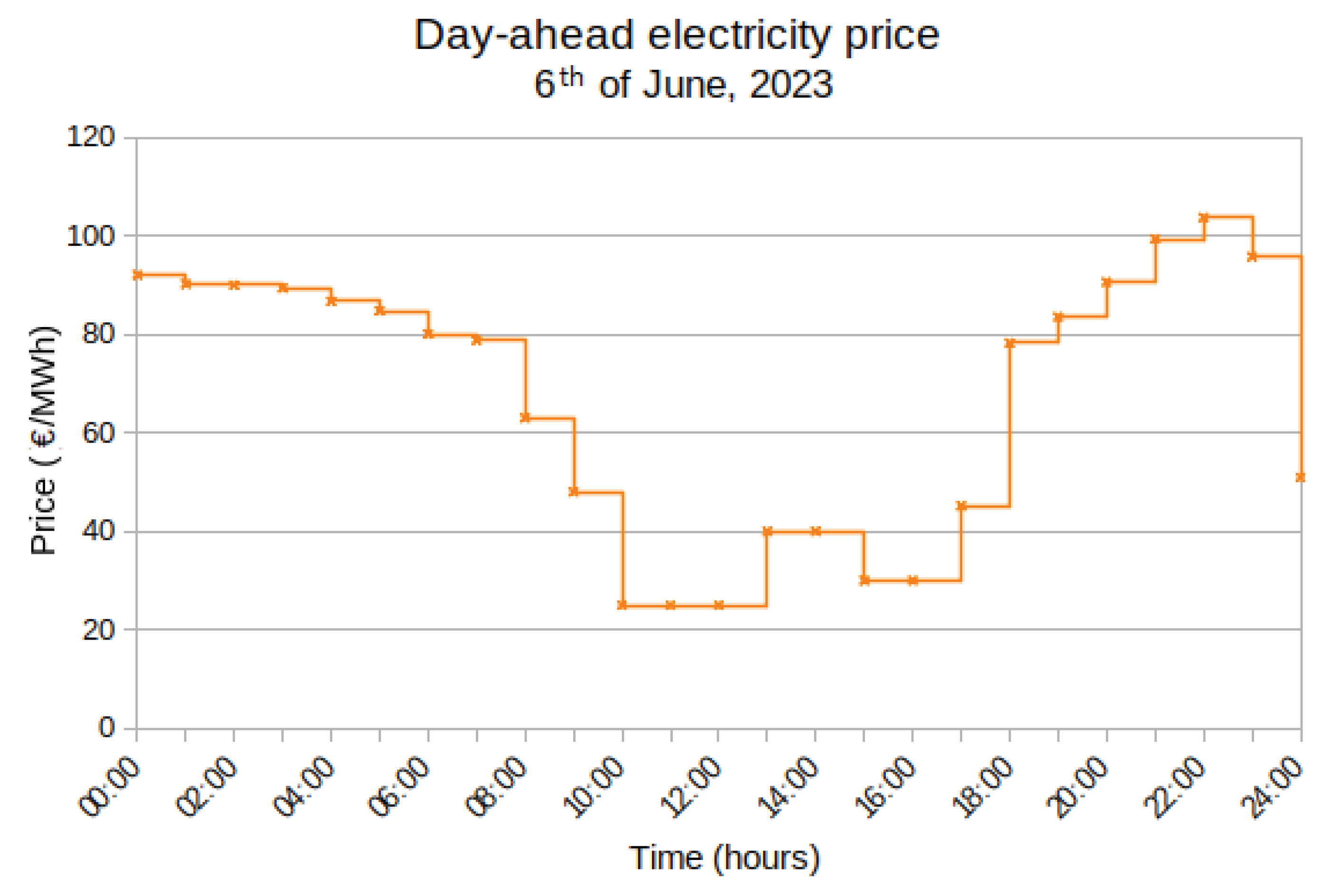
Before discussing the optimal control problem formulation in detail, two crucial components are defined: the price time series, which determines the electricity price per MWh, and the objective functional, which describes the profits considering the battery’s degradation.

3.1. Price Time Series

The European power market has two different pricing systems for buying and selling electricity. This policy states that electricity can be purchased more expensive in the balancing market compared to the day-ahead market. Conversely, electricity can be sold at a lower price in the balancing market compared with the day-ahead market [31]. The key is to maintain the grid balanced at all times. Since the imbalance costs are unavoidable, the operator must plan the price submissions carefully as they can incur higher prices due to the imbalances. This market approach facilitates transactions for electrical energy by allowing generating company agents to submit bids for buying and selling energy for the following day. The market session occurs daily at noon Central European Time, where prices and energy volumes are determined for the next twenty-four hours. The intersection of supply and demand defines the price and energy volume for a particular hour. Therefore, price information for the day-ahead market is essential to plan market transactions that will occur the next day.

For this study, we have taken a more straightforward method compared to the approach discussed in reference [30]. In that reference, the analysis involves complex definitions of electricity pricing and extending the scope beyond the day-ahead window, which makes the solution more complicated. We focused on the 24-hour period, during which the price of the electricity was clearly defined. For the sake of simulation simplicity, we assumed that the initial state of charge (

S_{o C}

) of the battery was 42%. The price time series for this study is presented in Figure 1. The figure shows the day-ahead electricity price in euros/MWh from 00:00 to 23:59 on June

6^{th}

, 2023, at precisely 1-hour intervals. The day-ahead electricity price for 2023 is available for download from the official European Network of Transmission System Operators website [32].

3.2. Formulation of Dynamic Models

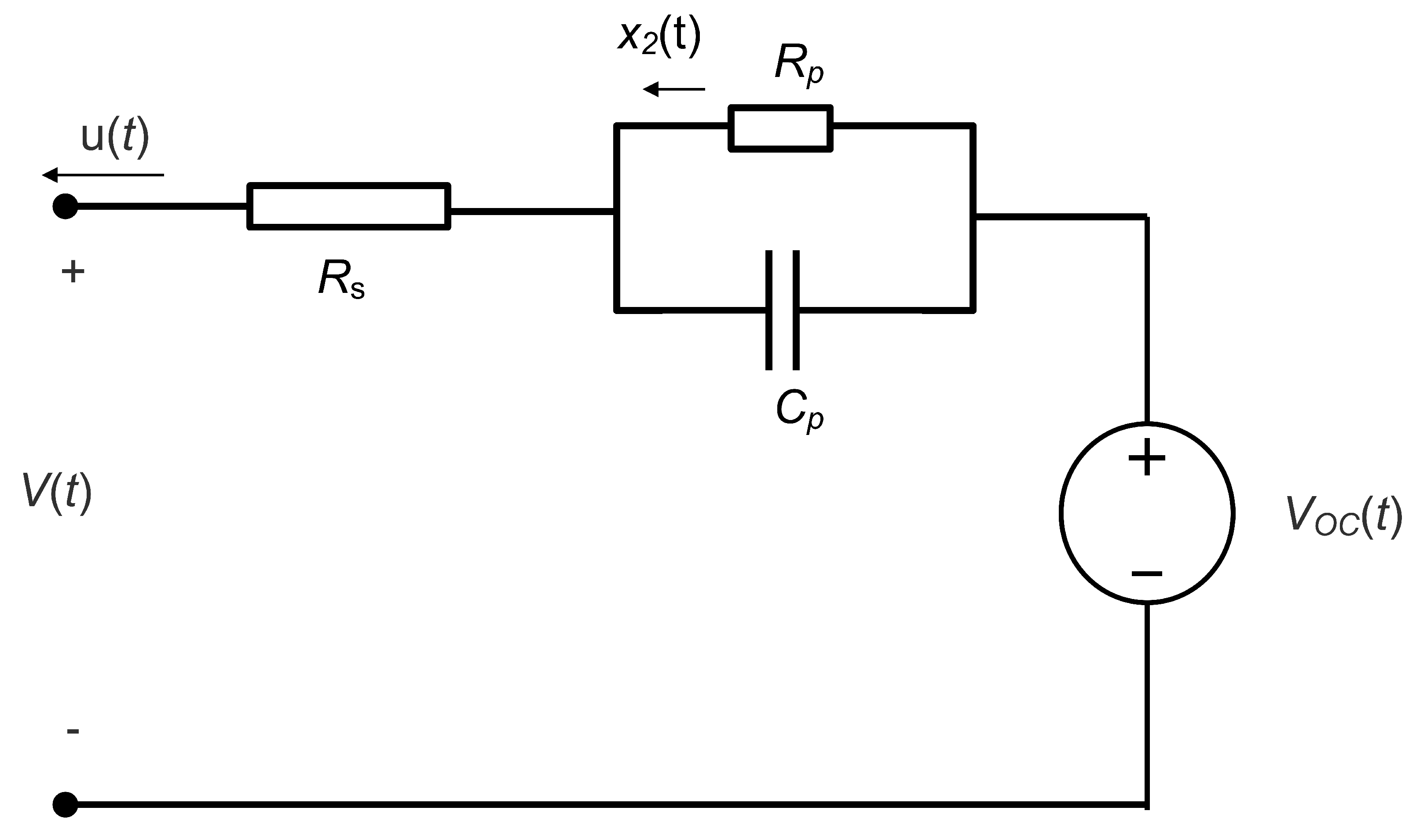
As shown in Figure 2, an equivalent circuit model was postulated to formulate the empirical model with degradation. The equivalent circuit model does not rely on any thermal model to incorporate temperature effects. Its holistic approach considers these effects embedded in the experimental data. This model achieves enough accuracy to estimate the output voltage, load current and power flow. It also maintains a manageable computational complexity to predict internal degradation.

The state vector used to describe the equivalent circuit model is

x (t) = {[x_{1} x_{2} x_{3} x_{4} x_{5}]}^{T}

where

x_{1}

is the state of charge,

x_{2}

is the current through the resistance

R_{p}

(A),

x_{3}

x_{4}

and

x_{5}

are extra states used to determine quantities of interest, as described below. The control variable u is the current from the battery (A). The convention used in the model implies that u is positive when the battery is discharging and negative when it is charging.

The model was partially extracted from [6] and augmented with three new state variables, namely

x_{3}

x_{4}

and

x_{5}

, as shown in Equation (6):

\begin{matrix} {\dot{x}}_{1} (t) & = \frac{u (t)}{C_{d e g} (t) C} \\ {\dot{x}}_{2} (t) & = 3600 (\frac{u (t)}{R_{p} C_{p}} - \frac{x_{2} (t)}{R_{p} C_{p}}) \\ {\dot{x}}_{3} (t) & = V {(t)}^{2} \\ {\dot{x}}_{4} (t) & = V (t) \\ {\dot{x}}_{5} (t) & = | u (t) | \end{matrix}

(6)

where C is the nominal battery capacity in Ah,

C_{d e g}

is the capacity degradation factor of Equation (5), and

V (t)

is the voltage across the battery terminals, given in Equation (7):

V (t) = V_{O C} (x_{1} (t)) - x_{2} (t) R_{p} - u (t) R_{d e g} (t) R_{s}

(7)

where

V_{O C}

is function used to estimate the internal voltage,

R_{d e g}

is a degradation factor given in Equation (5), and

R_{s}

is the internal battery resistance. The time dependency of the degradation factors

C_{d e g}

and

R_{d e g}

is highlighted, as both of them depend of the electric charge Q passing through the battery, which varies with time.

The state of charge versus

V_{O C}

curve for an 18650 Li(NiMnCo)O₂ battery cell data was sourced from reference [33]. The data were digitalised, and a 7^th-order polynomial was used to fit the curve. Typical values for

R_{p}, R_{s}

, and

C_{p}

are:

R_{p}

=15.80

\cdot 10^{- 3} Ω

R_{s}

= 8.2

\cdot 10^{- 3} Ω

and

C_{p}

= 38

k F

[34]. The transient behaviour of the lithium-ion cell is characterised by the product of

R_{p}

and

C_{p}

[35].

States

x_{3}

x_{4}

and

x_{5}

are state variables required to estimate the RMS value of the terminal voltage ,

V_{r m s}

, the mean value of the terminal voltage

V_{m e a n}

, and the total charge going through the battery,

Q (t)

, which is calculated as the integral of

| u (t) |

, as follows:

V_{r m s} = \sqrt{\frac{1}{t_{f}} \int_{0}^{t_{f}} V^{2} (t) d t} = \sqrt{\frac{x_{3} (t_{f})}{t_{f}}}

(8)

V_{m e a n} = \frac{1}{t_{f}} \int_{0}^{t_{f}} V (t) d t = \frac{x_{4} (t_{f})}{t_{f}}

(9)

Q (t) = \int_{0}^{t} | u (τ) | d τ = x_{5} (t)

(10)

3.3. Empirical Degradation Parameters

The research object of this work is the Sanyo UR18650E lithium-ion battery cell (Sanyo Electric Co., Ltd., Osaka, Japan), which has a cylindrical shape. According to the manufacturer, this cell is rated at

C = 2.1

± 0.05 Ah, and its nominal voltage is 3.6 V. The cathode active material consists of Li(NiMnCo)O₂, and the anode material is made of graphite. The grid-connected battery energy storage system modelled in this work is assumed to be composed of 750 UR18650E battery cells, with a total nominal energy storage capacity of 5.67 kWh. The battery cells were assumed to be arranged in a series/parallel configuration. It is important to note that although the cells are assumed to behave identically to simplify the analysis, slight differences in behaviour have been observed even among cells from the same production batch [36].

The empirical degradation model considers two crucial factors: battery cycling and calendar ageing. The model was extracted from [30], also using information from [20]. The model is based on the approach from Liaw et al. [37] in which a relatively simple equivalent circuit model simulates the battery performance and life cycling using a coupled thermal ageing model. However, all nonlinear parameters in the model were determined through empirical means. In the tests presented in [20], the authors found two different dependencies during cycling ageing analysis. One related to capacity reduction, or

C_{d e g}

and one to internal resistance increase,

R_{d e g}

All the experimental data regarding battery capacity fading and resistance degradation used in this work was extracted from reference [20]. However, all the curve fitting procedures have been revisited, and improvements in the fitting quality have been implemented, as explained below.

To begin with, we examined the reduction of battery capacity due to battery cycling. The relationship between the capacity reduction during battery cycling and the charge that passes through the battery is determined by Equation (1). On the other hand, the increase of resistance during battery cycling and the charge passing through the battery is determined by Equation (3). The experimental data set to estimate the parameter

β_{c a p}

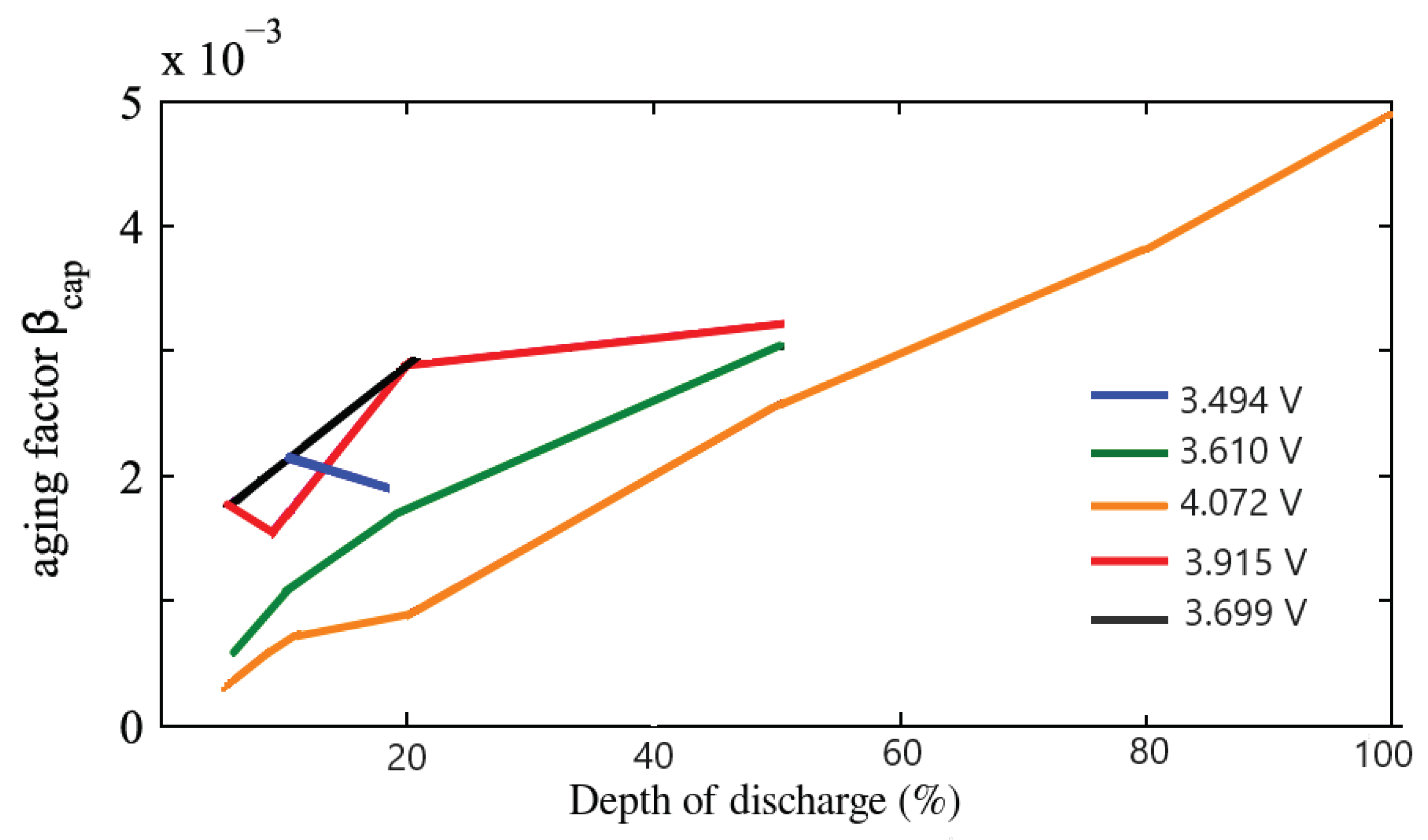
was digitally extracted from Figure 11 of reference [20]. The data points are shown in Table 1. The data showed that

β_{c a p}

is strongly dependent on both the average battery voltage (

V_{m e a n}

) and the depth of discharge

D_{o d}

as shown in Figure 3.

In reference [20], the author proposed a method for effectively linking the parameters

β_{c a p}

and

β_{r e s}

with the voltage and depth of discharge. They suggested a linear function combined with a quadratic function. While this approach is reasonably accurate, we chose to use a different methodology. We opted for the bilinear interpolation function, a feature provided by PSOPT, optimal control solver used in this work [38]. We sampled the data based on voltage and depth of discharge, and the data points are presented in Table 1.

Second, we consider degradation in the capacity via calendar ageing. Here, the battery capacity varies with time, particularly with

t^{0.75}

, according to the Equation (3). The calendar ageing data showed that

α_{c a p}

and

α_{r e s}

strongly depend on the average battery voltage and the cell temperature T. Therefore, they can be approximated using a single two-variable interpolation function to fit both dependencies simultaneously.

It can intuitively be observed from the graphs that

α

is linearly dependent on the voltage and follows the Arrhenius formula for temperature dependency according to the following equations:

\begin{matrix} α_{V} (V) & = a_{1} \cdot V + a_{2} \end{matrix}

(11)

\begin{matrix} α_{T} (T) & = a_{3} \cdot exp (- \frac{E_{a}}{R T}) \end{matrix}

(12)

where the variables

E_{a}

, T and R are the activation energy, temperature in Kelvin and the universal gas constant, respectively. The parameter

α_{c a p}

is a combination of both results as shown in Equation (13):

\begin{matrix} α_{c a p} & = (a_{1} \cdot V + a_{2}) [a_{3} \cdot exp (- \frac{E_{a}}{R T})] \end{matrix}

(13)

Equation (12) can be transformed into a linear function using the natural logarithm function, as shown in Equation (14)

\begin{matrix} ln α_{T} (T) = ln a_{3} + E_{a} {(R T)}^{- 1} \end{matrix}

(14)

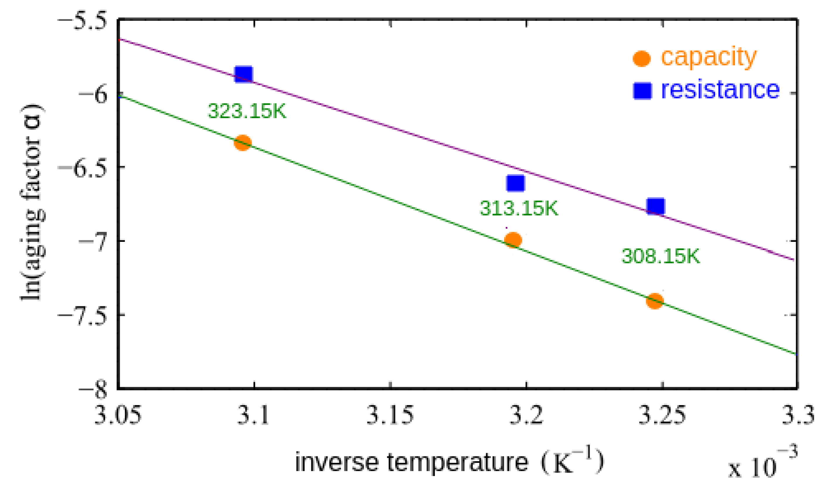
The experimental data set to estimate the parameter

α_{c a p}

and

α_{r e s}

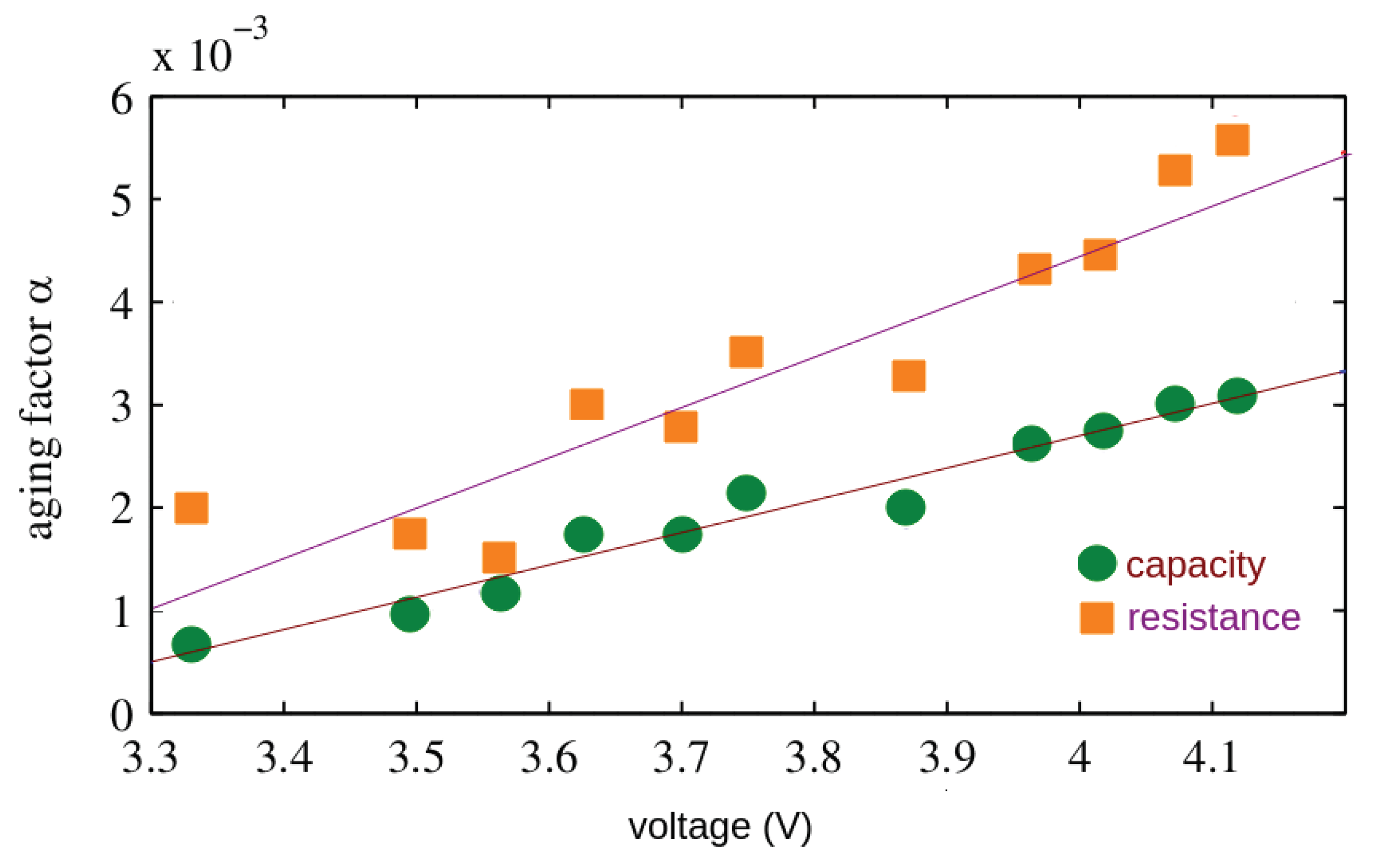
for the linear case was digitally extracted from Figure 8 in reference [20] and is shown in Figure 4.

Employing linear regression (the brown line in the figure) has yielded the subsequent linear approximation:

\begin{matrix} α_{V} (V) & = 0.0031566 \cdot V - 0.0099464 \end{matrix}

(15)

Similarly, the experimental data set to estimate the parameter

α_{c a p}

and

α_{r e s}

for the exponential case was digitally extracted from Figure 9 in reference [20] and is plotted in natural logarithm scale in Figure 5.

For the temperature dependency, using the data points shown in Figure 5 to produce a linear interpolation (green line), and employing linear regression has yielded the subsequent linear approximation:

\begin{matrix} \ln α_{T} (T) & = 15.1882 - 6960.00 T^{- 1} \end{matrix}

(16)

and finally, the parameter

α_{T} (T)

is given in Equation (17):

\begin{matrix} α_{T} (T) & = 3.94 \times 10^{6} \cdot \exp (- \frac{6960.00}{T}) \end{matrix}

(17)

Equations (15) and (17) cannot be combined into a single equation, as suggested in Equation (13), because the two fitting functions,

α_{T} (T)

and

α_{V} (V)

, do not match precisely for all the experimental data. Therefore, we will use the technique proposed in reference [20]. The approach is to average

α_{T} (T)

and

α_{V} (V)

at the temperature of

323.15 K

, where the two experimental curves intersect. The resulting value is named

α_{ϕ}

and it is used for scaling both fitting functions is a single one. Then apply this scale factor to the final

α_{c a p}

equation.

From Figure 4,

α_{V} (3.699 V)

at T=

323.15 K

is 0.0016368, and from Figure 5,

α_{T} (323.15 K)

is 0.0001746702. Hence, the scale factor applied to

α_{c a p}

is given in Equation (18):

\begin{matrix} α_{ϕ} = \frac{α_{V} (3.699 V) + α_{T} (323.15 K)}{2} = 0.001691751 \end{matrix}

(18)

Applying the scale factor to

α_{T} (T)

and

α_{V} (V)

\begin{matrix} α_{T, s c a l e d} & = α_{T} (T) \frac{α_{ϕ}}{α_{T} (323.15 K)} \end{matrix}

(19)

\begin{matrix} α_{V, s c a l e d} & = α_{V} (V) \frac{α_{ϕ}}{α_{V} (3.699)} \end{matrix}

(20)

The resulting scale factor that needs to be applied to the fitting function

α_{c a p}

is given in Equation (21):

\begin{matrix} α_{c a p} (V, T) & = \frac{α_{V} (V) \cdot α_{T} (T) \cdot α_{ϕ}}{α_{V} (3.699 V) \cdot α_{T} (323.15 K)} \end{matrix}

(21)

\begin{matrix} = 591.7278766 \cdot α_{V} (V) \cdot α_{T} (T) \end{matrix}

(22)

By combining equations (15) and (17) with (22), the final expression for

α_{c a p} (V, T)

is given in equation (23):

\begin{matrix} α_{c a p} (V, T) = (7.364999 \cdot V - 23.21504) exp (- \frac{6960.00}{T}) \times 10^{6} \end{matrix}

(23)

The estimation of the total capacity lost considering cycling ageing and calendar ageing is the superposition of the

C_{a g e}

as shown in Equation (1) and

C_{c y l}

as shown in Equation (3).

A similar procedure was applied to find the values for degradation in the resistance,

R_{d e g}

. The experimental data set to estimate the parameter

β_{r e s}

was digitally extracted from Figure 12 ( b) of reference [20]. We used a bilinear interpolation function, which is provided in the optimal control solver, PSOPT. The data was sampled for different values of voltage and depth of discharge. The data points are shown in Table 2.

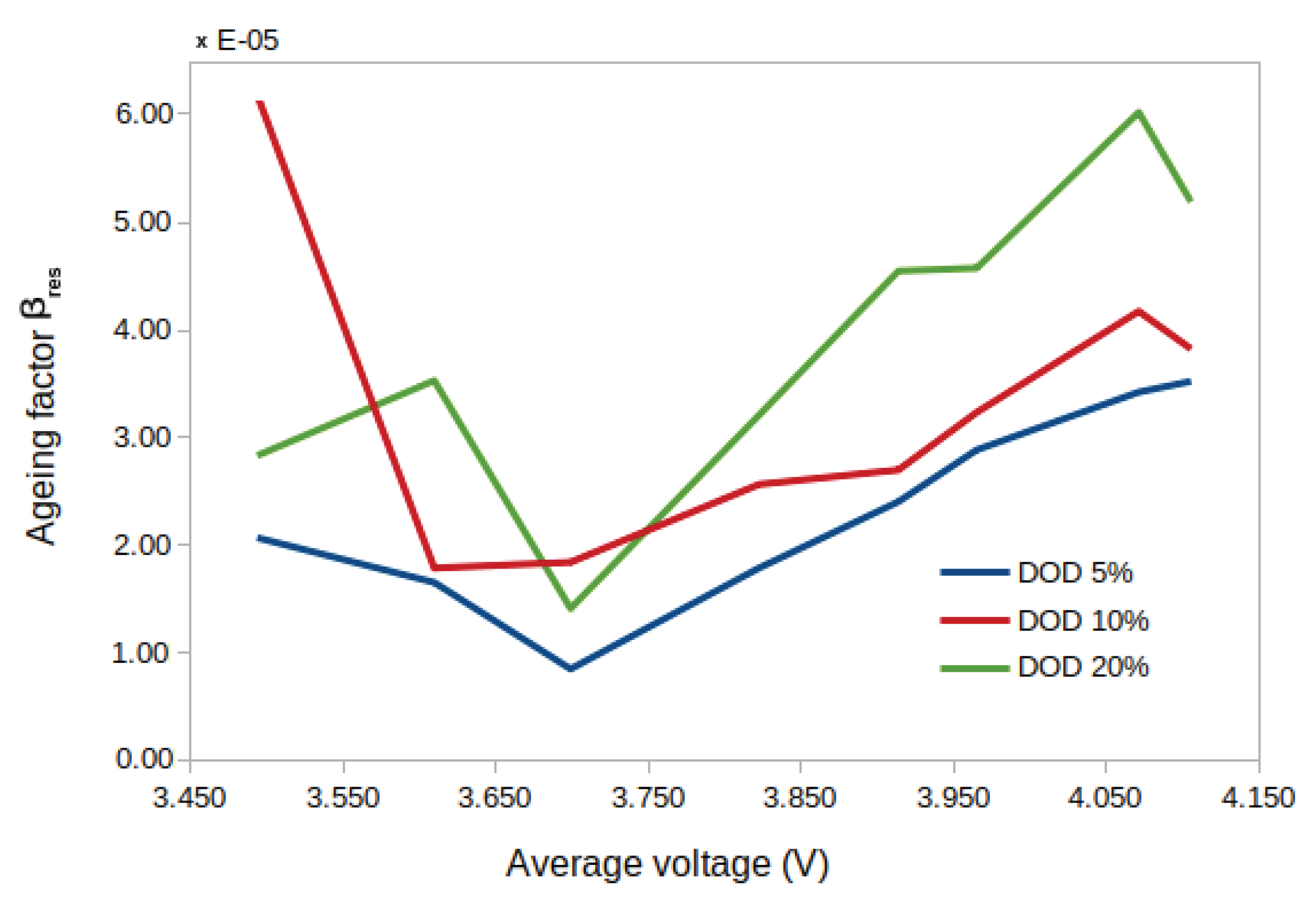
The data showed that

β_{r e s}

is strongly dependent on both the average battery voltage (

V_{m e a n}

) and the depth of discharge

D_{o d}

as shown in Figure 6.

To obtain

α_{r e s}

, we followed the same steps as before, with

α_{ϕ}

being defined in Equation (18). The data points are shown in Figure 4 and Figure 5. Equation (24) provides the expression for

α_{r e s}

\begin{matrix} α_{r e s} (V, T) = (5.270 \cdot V - 16.32) exp (- \frac{5986.00}{T}) \times 10^{5} \end{matrix}

(24)

The estimation of the total resistance increase considering battery cycling and calendar ageing is the superposition of the

R_{c y l}

as shown in Equation (2) and

R_{a g e}

as shown in Equation (4).

3.4. Objective functional derivation

The objective functional, J, in Bolza form for the empirical model, as shown in equation (25).

\begin{matrix} J = - C_{d e g} (u (\cdot), x (\cdot)) + \int_{0}^{t_{f}} R_{e v} (u (t), x (t)) d t \end{matrix}

(25)

where u is the control variable, which is the current from the battery,

x

is the state vector,

t_{f}

is the final time, and

R_{e v}

is the revenue (or cost of energy purchase) per unit of time, given by Equation (26)

\begin{matrix} R_{e v} (u (t), x (t)) = u (t) V (t) π (t) N \times 10^{- 6} \end{matrix}

(26)

where

V (t)

is the voltage defined in equation (7),

π (t)

is a known price function that represents the actual price of energy in euros/MWh at time t, N is the number of cells, and the

10^{- 6}

factor converts the electricity price from /MWh to /Wh. Similarly,

C_{d e g}

is the degradation cost defined by Equation (27)

\begin{matrix} C_{d e g} (u (\cdot), x (\cdot)) = E_{l o s t, W h} δ_{d e g} N \end{matrix}

(27)

where

E_{l o s t, W h}

is defined in Equation (28):

\begin{matrix} E_{l o s t, W h} = [α_{c a p} (V_{m e a n}, T_{a}) t_{f}^{0.75} + β (V_{r m s}, Δ D) \sqrt{\int_{0}^{t_{f}} | u (t) | d t}] E_{A h} \end{matrix}

(28)

where

T_{a} = 298.5

K is the ambient temperature. As our mathematical model does not include a coupled thermal model, we approximated the average temperature during the charging cycle in the empirical equations as the ambient temperature. Substituting Equation (28) into Equation (27), then J is given in Equation (29):

\begin{matrix} J = - [α_{c a p} (V_{m e a n}, T_{a}) t_{f}^{0.75} + β (V_{r m s}, Δ D) \sqrt{\int_{0}^{t_{f}} | u (t) | d t}] E_{A h} δ_{d e g} N a + \\ \int_{0}^{t_{f}} u (t) V (t) 10^{- 6} π (t) N d t \end{matrix}

(29)

where the meaning of the variables and parameters in Equation (29) is given in Table 3.

4. Optimal Control Problem Formulation

The problem is formulated as a single-phase optimal control problem, with the phase contained in the time interval

t \in [t_{0}, t_{f}]

, where

t_{0}

and

t_{f}

are fixed. The aim is to find the control trajectory

u (t)

t \in [t_{0}, t_{f}]

, and the state trajectory , x

(t)

t \in [t_{0}, t_{f}]

, that minimises the objective functional, J, expressed in Equation (30), given the dynamics of the battery described in Equation (6).

\begin{matrix} J = - (α_{c a p} (V_{m e a n}, T_{a}) \cdot {(t_{f} / 24)}^{0.75} + β_{c a p} (V_{r m s}, Δ D) \cdot \sqrt{x_{5} (t_{f})}) E_{A h} δ_{d e g} N + \\ \int_{0}^{t_{f}} u (t) V (t) 10^{- 6} π (t) N d t \end{matrix}

(30)

where

V (t)

is defined in Equation (7), and

Δ D = D_{o d}^{m a x} - D_{o d}^{m i n}

. The bounds for the states and the control are given in Equation (31) :

\begin{matrix} 0.1 & \leq x_{1} \leq 0.85 \\ - I_{\max} & \leq x_{2} \leq I_{\max} \\ 0.0 & \leq x_{3} \leq t_{f} V_{mean}^{2} \\ 0.0 & \leq x_{4} \leq t_{f} V_{mean} \\ 0.0 & \leq x_{5} \leq t_{f} I_{\max} \\ - I_{\max} & \leq u \leq I_{\max} \end{matrix}

(31)

where

I_{\max}

is the maximum current from the cell in one hour.

A path constraint is included to prevent under/over voltage damage, given in Equation (32):

\begin{matrix} 2.7 \leq V (t) \leq 4.2 \end{matrix}

(32)

The initial condition for the state vector is given in Equation (33):

\begin{matrix} x (0) & = {[0.42, 0.0, 0.0, 0.0, 0.0]}^{T} \end{matrix}

(33)

and

t_{f} = 24

hours is fixed.

4.1. Direct Numerical Methods for Optimal Control

Typically, with a few exceptions, optimal control problems are solved using numerical methods. In this work, we chose to use direct methods for optimal control as they offer several advantages over other approaches, as discussed in [39]. Direct methods for optimal control involve discretising the differential equations, constraints, and objective function associated with the problem, and the numerical optimisation of the resulting nonlinear programming problem. Usually, nonlinear programming (NLP) methods are used for solving the resulting nonlinear programming problem. Different methods can be used to discretise the differential equations, constraints and objective function, as discussed below.

Collocation methods consider the states and control variables as optimisation parameters, and the system of ODEs is regarded as nonlinear equality constraints in the discretised formulation. Then, a general NLP solver can produce a numerical solution to the discretised optimal control problem [40]. There are various approaches to collocation, but primarily, they can be divided into two groups. The first one is grounded on an implicit k-state Runge-Kutta scheme, as described in [39,41]. Euler, trapezoidal and Hermite-Simpson are among the most widely used collocation methods, which use linear, quadratic, and cubic polynomial interpolation, respectively.

Suppose that the differential equations involved in the optimal control problem of interest consist of a set of state equations described as follows:

\dot{x} (t) = f (x (t), u (t), t)

(34)

where

x : [t_{0}, t_{f}] \to R^{n}

defines the trajectory of the vector of state variables,

u : [t_{0}, t_{f}] \to R^{m}

defines the trajectory of the vector of control variables, t represents time,

[t_{0}, t_{f}], t_{f} > t_{0}

is a time interval,

f : R^{n} \times R^{m} \times [t_{0}, t_{f}] \to R^{n}

is a vector function that defines the state equations. Assume that a set of discretisation points is defined as follows:

{t_{0}, t_{1}, t_{2}, \dots t_{M}}

, where

t_{M} \equiv t_{f}

, and M is an integer number. For a given integer

i \in [0, M - 1]

, the discretisation step

h_{i}

is defined as

h_{i} = t_{i + 1} - t_{i}

. Also define

f_{i} = f (x (t_{i}), u (t_{i}), t_{i})

, and

f_{i + 1} = f (x (t_{i + 1}), u (t_{i + 1}), t_{i + 1})

Euler’s method, which is based on a linear interpolation polynomial, is the simplest collocation method and is given in Equation (35),

x_{i + 1} = x_{i} + h_{i} f_{i}

(35)

The trapezoidal approach is based on a quadratic interpolant polynomial, and is shown in Equation (36).

x_{i + 1} = x_{i} + \frac{h_{i}}{2} (f_{i} + f_{i + 1})

(36)

Lastly, the Hermite-Simpson scheme is based on a cubic interpolant polynomial and is described by Equation (37)

\begin{matrix} \bar{x} & = \frac{1}{2} (x_{i} + x_{i + 1}) + \frac{h_{i}}{8} (f_{i} - f_{i + 1}) \\ \bar{f} & = (\bar{x}, t_{i} + \frac{h_{i}}{2}) \\ x_{i + 1} & = x_{i} + \frac{h_{i}}{6} (f_{i} + 4 \bar{f} + f_{i + 1}) \end{matrix}

(37)

Numerous studies have been reported in the literature investigating the use of collocation techniques in optimal control problems based on either the Runge-Kutta or orthogonal polynomials approach. The approach has proven highly successful and is broadly applied across various engineering applications. These applications include, for example, trajectory optimisation problems [42,43,44,45], stabilization of complex trajectories for robots [46,47,48], minimum time low-thrust spacecraft orbit transfer [49], spacecraft proximity rendezvous [50] and lunar soft landing [51].

Only a few authors have explored the use of collocation methods to solve optimal control problems associated with battery storage systems. A discussion paper [52] formulated a discretised optimal control problem to examine the influence that energy storage can have on energy generation and investment decisions. The problem was solved using Chebyshev collocation methods and dynamic programming. In [53], orthogonal polynomials were used to estimate the optimal control strategy for a hybrid storage configuration composed of batteries and ultra-capacitors. Recent work [54] has addressed the optimal charging profile for a hybrid electric vehicle using an orthogonal collocation approach [55].

5. Results and Discussion

This study attempts to determine the battery operation over time that yields the optimal day-ahead energy dispatch by utilising market data from 6^th June 2023. The measure to determine the solution quality used in this work is the maximum relative local error [56]. As mentioned, the day-ahead electricity price data has been sourced from [32].

The problem was solved using mesh refinement with trapezoidal/Hermite-Simpson collocation methods. The mesh refinement algorithm was configured to perform up to seven iterations. Mesh refinement involves adjusting the mesh defined by the discresation points by efficiently subdividing the existing cells into smaller ones in sections of the time domain where accuracy needs to be improved, resulting in a higher number of cells and a finer representation of the problem domain. This process allows for a more precise approximation of the control and state variables over the time domain of the problem. By refining the mesh, finer details and variations in the control and state variables can be captured, leading to more accurate optimisation results. However, it is essential to strike a balance between the accuracy of the solution and computational cost.

5.1. Numerical Simulation

This section presents the outcomes of our in-depth refinement procedure to improve our computational simulations’ accuracy and resolution. We studied three cases, which are summarised in Table 4. We aimed to improve the maximum local relative error of the solutions and provide the best solution for each particular case. The price of electricity has been assumed constant within each hourly interval. Moreover, we assumed that the battery cells were not degraded at the beginning of the 24-hour window.

5.2. Solver Configuration

All computations were carried out using the optimal control software PSOPT Version 5.0. PSOPT [57] is an open-source, optimal control solver written in C++. The key parameters that define the solver configuration given in Table 5.

5.3. Simulation Results

Table 6 shows a summary of key results for the three cases, including the profit, net revenues, degradation cost, and the maximum relative local error achieved. The next few subsections additional provide details on the results obtained for each case, including the mesh refinements process, providing additional insights into the accuracy and resolution of the simulations, the state of charge profile, the optimal current profile and the terminal voltage profile.

5.3.1. Case 1: Maximising Net Revenues

In this case, net revenues are maximised, the cost of degradation is ignored, the model state equations do not include degradation, and the internal resistance value is not considered to increase because of degradation effects. Table 7 shows the mesh refinement results. The best maximum relative local error is

5.099 \times 10^{- 3}

obtained for iteration seven, with a total number of discretisation points of 845. Table 6 shows the optimal profit obtained for this case, corresponding to €7.82

\times 10^{- 1}

Figure 7 shows the resulting state of charge over time in this case. Figure 8 displays the optimal current profile. The battery is charged at the beginning of the day and reaches 85% in about 1 hour. Following that, for the next 10 hours, the battery remains essentially unused. Between 11 hours and 17 hours, the battery goes through a charge/discharge cycle, then stays discharged until 22 hours, when it starts charging again to about 85%.

The voltage at the terminals is shown in Figure 9. Notice that the voltage increases/decreases as the battery charges/discharges and that the voltage path constraint is respected.

5.3.2. Case 2: Maximising Profits without Considering Degradation in the Internal Resistance

In this case, profits are maximised, where profits are defined as net revenue minus cost of battery degradation, the state equations include the effect of degradation in capacity, while the internal resistance of the battery is not considered to increase because of degradation effects. Table 8 shows the mesh refinement results for this case. The best maximum relative local error is 9.5225

\times 10^{- 4}

obtained with a total number of discretisation points of 668.

Figure 10 shows the resulting state of charge over time. Figure 11 shows the optimal current profile for this case. Table 6 shows the optimal profit obtained for this case, which corresponds to €4.769

\times 10^{- 1}

. The same table shows the net revenues and the cost of degradation for this case.

In this case, the battery is partially charged to about 80% after one hour and then charges more slowly reaching 85% at about 5 hours, and then it stays inactive until about 10 hours. Between 10 hours and 13 hours, the battery fully discharges, then charges again to about 85% at 15 hours, then it starts discharging again until about 17 hours. It remains discharged until about 21 hours, when it starts to charge again to about 85% as the price of electricity starts reducing, making it cheaper to buy electricity from the grid. The terminal voltage profile for case 2 is shown in Figure 12.

5.3.3. Case 3: Maximising Profits Considering Degradation in the Internal Resistance

In this case, profits are maximised, where profits are defined as net revenue minus cost of battery degradation, the state equations include the effect of degradation in capacity, while the internal resistance of the battery is considered to increase because of degradation effects. The results of the mesh refinement procedure are shown in Table 9. The best maximum relative local error is 2.372

\times 10^{- 3}

obtained with total discretisation points of 671.

Table 6 shows the optimal profit obtained for this case, which corresponds to 4.768

\times 10^{- 1}

. The same table shows the net revenue and the cost of degradation associated to this case. Figure 13 shows the resulting state of charge over time. Figure 14 shows the optimal current profile. The results are very similar to those obtained in case 2; for instance, the profit values of cases 1 and 2 are only different in the third decimal digit, which indicates that introducing degradation to the internal resistance has a negligible effect on the profit value. The terminal voltage profile for case 3 is shown in Figure 15.

6. Conclusions

This work discussed the application of optimal control methods to optimise the participation of lithium-ion batteries in the day-ahead electricity market. Three cases were studied: maximising net revenues without consideration of degradation, maximising profits with consideration of capacity degradation, and maximising profits with consideration of degradation affecting both the battery’s capacity and the internal resistance. The study aimed to determine the optimal charge and discharge schedules for each case considering a 24-hour price profile from Belgium’s day-ahead electricity market.

The results show that, while the resulting charge/discharge profiles in are similar in the three cases, consideration of capacity degradation in the dynamics and objective function reduces profits, while also including the increase of internal resistance due to degradation resulted in a very small reduction in the profit value for the scenario considered in this work.

Two areas for further research include the incorporation of a thermal model into the state equations so that temperature effects on degradation can be more accurately modelled, and the validation of the optimal control methods presented here on a real battery energy storage system that participates in the day-ahead electricity market. Experimental validation will provide a further understanding of the real world applicability of the proposed methods beyond the simulation-based studies presented in this work.

Author Contributions

Conceptualisation, J.G.-S. and V.M.B.; methodology, J.G.-S.; software, J.G.-S.; validation, J.G.-S. and V.M.B.; formal analysis, J.G.-S.; investigation, J.G.-S.; resources, J.G.-S. and V.M.B.; writing—original draft preparation, J.G.-S.; writing—review and editing, V.M.B.; visualisation, J.G.-S.; supervision, V.M.B. All authors have read and agreed to the published version of the manuscript.

Funding

“This research received no external funding”.

Data Availability Statement

The data presented in this study are available on request from the corresponding author. The data are not publicly available due to the first author's PhD thesis not having been submitted at the time of publication of this work.

Conflicts of Interest

The authors declare no conflict of interest.

References

European Commission. Electricity market design. https://energy.ec.europa.eu/topics/markets-and-consumers/market-legislation/electricity-market-design_en Accessed on 26 of September 2023.
Gonzáles, N.; da Graça, M. Improving the design of the EU electricity market. 2023. https://www.europarl.europa.eu/RegData/etudes/BRIE/2023/745694/EPRS_BRI(2023)745694_EN.pdf Accessed on 18 of September 2023.
Divya Asija, R.V. Renewable energy integration in modern deregulated power system: challenges, driving forces, and lessons for future road map. In Advances in Smart Grid Power System: Network, Control and Security; Tomar, A., Kandari, R., Eds.; Academic Press: Oxford, United Kingdom, 2020; chapter 13; pp. 365–385. [Google Scholar]
Motamedi Sedeh, O.; Ostadi, B. Optimization of bidding strategy in the day-ahead market by consideration of seasonality trend of the market spot price. Energy Policy 2020, 145, 111740. [Google Scholar] [CrossRef]
Teleke, S. Control Methods for Energy Storage for Dispatching Intermittent Renewable Energy Sources. PhD thesis, University of North Carolina, Raleigh, 2009. [Google Scholar]
Reniers, J. Degradation-aware optimal control of grid-connected lithium-ion batteries. PhD thesis, Oxford University, Oxford, 2020.
Perez, H.E.; Hu, X.; Dey, S.; Moura, S.J. Optimal Charging of Li-Ion Batteries with Coupled Electro-Thermal-Aging Dynamics. IEEE Trans. Veh. Technol. 2017, 66, 7761–7770. [Google Scholar] [CrossRef]
Zheng, L.; Zhou, X.; Qiu, Q.; Yang, L. Day-ahead optimal dispatch of an integrated energy system considering time-frequency characteristics of renewable energy source output. Energy 2020, 209, 118434. [Google Scholar] [CrossRef]
Zhang, M.; Li, W.; Yu, S.S.; Wen, K.; Muyeen, S. Day-ahead optimization dispatch strategy for large-scale battery energy storage considering multiple regulation and prediction failures. Energy 2023, 270, 126945. [Google Scholar] [CrossRef]
Fotopoulou, M.; Rakopoulos, D.; Blanas, O. Day Ahead Optimal Dispatch Schedule in a Smart Grid Containing Distributed Energy Resources and Electric Vehicles. Sensors 2021, 21, 218–222. [Google Scholar] [CrossRef] [PubMed]
Zhang, Z.; Wang, C.; Lv, H.; Liu, F.; Sheng, H.; Yang, M. Day-Ahead Optimal Dispatch for Integrated Energy System Considering Power-to-Gas and Dynamic Pipeline Networks. IEEE Trans. Ind. Appl. 2021, 57, 3317–3328. [Google Scholar] [CrossRef]
Akkas, O.P.; Cam, E. Optimal operational scheduling of a virtual power plant participating in day-ahead market with consideration of emission and battery degradation cost. Int. Trans. Electr. Energy Syst. 2020, 30, e12418. [Google Scholar] [CrossRef]
Fernández-Muñoz, D.; Pérez-Díaz, J.I. Optimisation models for the day-ahead energy and reserve self-scheduling of a hybrid wind–battery virtual power plant. J. Energy Storage 2023, 57, 106296. [Google Scholar] [CrossRef]
Hwang, Y.S.; Tan, Z.; Tan, Q.; Wang, Y. Bidding Strategy of Virtual Power Plant with Energy Storage Power Station and Photovoltaic and Wind Power. J. Engineering 2018, 2018. [Google Scholar]
Parastegari, M.; Hooshmand, R.A.; Khodabakhshian, A.; Zare, A.H. Joint operation of wind farm, photovoltaic, pump-storage and energy storage devices in energy and reserve markets. nt. J. Electr. Power Energy Syst. 2015, 64, 275–284. [Google Scholar] [CrossRef]
Akkas, O.P.; Cam, E. Optimal Control of Battery Energy Storage for Wind Farm Dispatching. IEEE T Energy Conver 2010, 25, 787–794. [Google Scholar]
Perriment, R.; Kumtepeli, V.; McCulloch, M.; Howey, D. Lead-acid battery lifetime extension in solar home systems under different operating conditions. In Proceedings of the Proceedings of the IEEE PES/IAS PowerAfrica; IEEE; 11; 2023. [Google Scholar]
Reiter, C.; Wildfeuer, L.; Wassiliadis, N.; Krahl, T.; Dirnecker, J.; Lienkamp, M. A Holistic Approach for Simulation and Evaluation of Electrical and Thermal Loads in Lithium-Ion Battery Systems. In Proceedings of the 2019 Fourteenth International Conference on Ecological Vehicles and Renewable Energies (EVER); 2019; pp. 1–17. [Google Scholar]
Reiter, C.; Lin, X.; Schlereth, L.; Lienkamp, M. Finding the ideal automotive battery concept. Forsch Ingenieurwes 2019, 83, 817–830. [Google Scholar] [CrossRef]
Schmalstieg, J.; Käbitz, S.; Ecker, M.; Sauer, D.U. A holistic aging model for Li(NiMnCo)O2 based 18650 lithium-ion batteries. J POWER SOURCES 2014, 257, 325–334. [Google Scholar] [CrossRef]
Zhang, H.; Liu, W.; Dong, Y.; Zhang, H.; Chen, H. A Method for Pre-determining the Optimal Remanufacturing Point of Lithium ion Batteries. Procedia CIRP 2014, 15, 218–222, 21st CIRP Conference on Life Cycle 69 Engineering. [Google Scholar] [CrossRef]
Takei, K.; Kumai, K.; Kobayashi, Y.; Miyashiro, H.; Terada, N.; Iwahori, T.; Tanaka, T. Cycle life estimation of lithium secondary battery by extrapolation method and accelerated aging test. J POWER SOURCES 2001, 97-98, 697–701, Proceedings of the 10th International Meeting on Lithium Batteries. [Google Scholar] [CrossRef]
Wang, J.; Liu, P.; Hicks-Garner, J.; Sherman, E.; Soukiazian, S.; Verbrugge, M.; Tataria, H.; Musser, J.; Finamore, P. Cycle-life model for graphite-LiFePO4 cells. J POWER SOURCES 2011, 196, 3942–3948. [Google Scholar] [CrossRef]
Paffumi, E.; De Gennaro, M.; Martini, G. In-vehicle battery capacity fade: A follow-up study on six European regions. Energy Reports 2024, 11, 817–829. [Google Scholar] [CrossRef]
Li, X.; Wang, Q.; Yang, Y.; Kang, J. Correlation between capacity loss and measurable parameters of lithium-ion batteries. Int. J. Electr. Power Energy Syst. 2019, 110, 819–826. [Google Scholar] [CrossRef]
Preger, Y.; Barkholtz1, H.M.; Fresquez, A.; Campbell, D.L.; Juba, B.W.; Romàn-Kustas, J.; Ferreira, S.R.; Chalamala, B. Degradation of Commercial Lithium-Ion Cells as a Function of Chemistry and Cycling Conditions. J ELECTROCHEM SOC 2020, 167, 120532, Proceedings of the 10th International Meeting on 89 Lithium Batteries. [Google Scholar] [CrossRef]
Mandli, A.R.; Kaushik, A.; Patil, R.S.; Naha, A.; Hariharan, K.S.; Kolake, S.M.; Han, S.; Choi, W. Analysis of the effect of resistance increase on the capacity fade of lithium ion batteries. Int. J. Energy Res. 2019, 43, 2044–2056. [Google Scholar] [CrossRef]
Krupp, A.; Beckmann, R.; Diekmann, T.; Ferg, E.; Schuldt, F.; Agert, C. Calendar aging model for lithium-ion batteries considering the influence of cell characterization. Journal of Energy Storage 2022, 45, 103506. [Google Scholar] [CrossRef]
Vetter, J.; Novák, P.; Wagner, M.; Veit, C.; Möller, K.C.; Besenhard, J.; Winter, M.; Wohlfahrt-Mehrens, M.; Vogler, C.; Hammouche, A. Ageing mechanisms in lithium-ion batteries. Journal of Power Sources 2005, 147, 269–281. [Google Scholar] [CrossRef]
Reniers, J.; Mulder, G.; Ober-Blöbaum, S.; Howey, D.A. Improving optimal control of grid-connected lithium-ion batteries through more accurate battery and degradation modelling. J POWER SOURCES 2018, 379, 91–102. [Google Scholar] [CrossRef]
Zhou, B.; Liu, X.; Cao, Y.; Li, C.; Chung, C.Y.; Chan, K.W. Optimal scheduling of virtual power plant with battery degradation cost. IET Optimal Utilisation of Storage Systems in Transmission and Distribution Systems 2016, 10, 712–725. [Google Scholar] [CrossRef]
ENTSO. ENTSO - transparency platform. 2023. https://transparency.entsoe.eu/dashboard/show Accessed on 18 of September 2023.
Jiang, H.; Chen, X.; Liu, Y.; Zhao, Q.; Chen, B. Online State-of-Charge Estimation Based on the Gas–Liquid Dynamics Model for Li(NiMnCo)O₂ Battery. Energies 2021, 14, 324–343. [Google Scholar] [CrossRef]
Plett, G. Battery Management Systems, Volume I: Battery Modeling; Artech House Publishers: Maryland, USA, 2015. [Google Scholar]
Su, J.; Lin, M.; Wang, S.; Li, J.; Coffie-Ken, J.; Xie, F. An equivalent circuit model analysis for the lithium-ion battery pack in pure electric vehicles. Measurement and Control 2019, 52, 193–201. [Google Scholar] [CrossRef]
Reniers, J.; Howey, D.A. Digital twin of a MWh-scale grid battery system for efficiency and degradation analysis. APPL ENERG 2023, 336, 120774. [Google Scholar] [CrossRef]
Liaw, B.Y.; Jungst, R.G.; Nagasubramanian, G.; Case, H.L.; Doughty, D.H. Modeling capacity fade in lithium-ion cells. J POWER SOURCES 2005, 140, 157–161. [Google Scholar] [CrossRef]
Becerra, V.M. PSOPT optimal control solver - User Manual (version 02.09.2022). 2022. https://github.com/PSOPT/psopt/blob/master/doc/PSOPT_Manual_R5.pdf Accessed 17 March 2024.
Betts, J. Practical Methods for Optimal Control and Estimation Using Nonlinear Programming, second ed.; SIAM: Philadelfia, 2010. [Google Scholar]
Hargraves, C.R.; Paris, S.W. Direct trajectory optimization using nonlinear programming and collocation. J Guid. Control Dynam. 1987, 10, 338–342. [Google Scholar] [CrossRef]
Pytlak, R. Numerical Methods for Optimal Control Problems with State Constraints; Springer Verlag: Warsaw, Poland, 1991. [Google Scholar]
Rao, A.V.; Tang, S.; Hallmank, W.P. Numerical optimization study of multiple-pass aeroassisted orbital transfer. Optim Control Appl. Methods 2002, 23, 215–238. [Google Scholar] [CrossRef]
Betts, J. Issues in the Direct Transcription of Optimal Control Problems to Sparse Nonlinear Programs. In Computational Optimal Control; Bulirsch, R., Kraft, D., Eds.; Birkhauser Verlag: Basel, Switzerland, 1994; chapter 1; pp. 3–18. [Google Scholar]
Chernousko, F. Optimization in Control of Robots. In Computational Optimal Control; Bulirsch, R., Kraft, D., Eds.; Birkhauser Verlag: Basel, Switzerland, 1994; chapter 2; pp. 19–28. [Google Scholar]
Gill, P.; Murray, W.; Saunders, M.A. Large-scale SQP Methods and their Application in Trajectory Optimization. In Computational Optimal, Control; Bulirsch, R., Kraft, D., Eds.; Birkhauser Verlag: Basel, Switzerland, 1994; chapter 2; pp. 29–42. [Google Scholar]
Posa, M.; Kuindersma, S.; Tedrake, R. Optimization and stabilization of trajectories for constrained dynamical systems. In Proceedings of the 2016 IEEE International Conference on Robotics and Automation (ICRA); 2016; pp. 1366–1373. [Google Scholar]
Dafarra, S.; Romualdi, G.; Pucci, D. Dynamic Complementarity Conditions and Whole-Body Trajectory Optimization for Humanoid Robot Locomotion. IEEE Trans. Robot. 2022, 38, 3414–3433. [Google Scholar] [CrossRef]
Bordalba, R.; Schoels, T.; Ros, L.; Porta, J.M.; Diehl, M. Direct Collocation Methods for Trajectory Optimization in Constrained Robotic Systems. IEEE Trans. Robot. 2023, 39, 183–202. [Google Scholar] [CrossRef]
Herman, A.L. Improved Collocation Methods With Application to Direct Trajectory Optimization. PhD thesis, University of Illinois Urbana-Champaign, 1995. [Google Scholar]
Liu, T.; Zhao, Y.S.; Shi, P.; Li, B.J. Trajectory Optimization for Spacecraft Proximity Rendezvous Using Direct Collocation Method. In Proceedings of the Materials Science and Information Technology. Trans Tech Publications Ltd, 2 2012, Vol. 433, Advanced Materials Research pp. 6652–6656.
Tu, L.; Yuan, J.; Luo, J.; Ning, X.; Zhou, R. Lunar soft landing rapid trajectory optimization using direct collocation method and nonlinear programming. In Proceedings of the Second International Conference on Space Information Technology; Wang, C., Zhong, S., Wei, J., Eds.; International Society for Optics and Photonics, SPIE, 2007; Vol. 6795, p. 67954T. [Google Scholar]
Durmaz, T. Energy storage and renewable energy. Technical report, Norwegian School of Economics. Department of Economics, 2014.
Li, J.; Fu, Z.; Jin, X. Rule Based Energy Management Strategy for a Battery/Ultra-capacitor Hybrid Energy Storage System Optimized by Pseudospectral Method. Energy Procedia 2017, 105, 2705–2711, 8th International Conference on Applied Energy, ICAE2016, 8-11 October 2016, Beijing, China. [Google Scholar] [CrossRef]
Multani, S.S. Pseudospectral Collocation Method Based Energy Management Scheme for a Parallel P2 Hybrid Electric Vehicle. Master's thesis, The Ohio State University, 2020. [Google Scholar]
Garg, D.; Patterson, M.; Hager, W.; Rao, A.; Benson, D.R. An overview of three pseudo-spectral methods for the numerical solution of optimal control problems. IEEE Trans. Robot. 2017; 1–18. [Google Scholar]
Betts, J. Practical Methods for Optimal Control and Estimation Using Nonlinear Programming, third edition ed.; SIAM: Philadelfia, 2020. [Google Scholar]
Becerra, V.M. PSOPT optimal control software. 2020. https://www.psopt.net/ Accessed 28 Nov 2022.

Figure 1. 24-hours day-ahead electricity price for the Belgium's market.

Figure 2. Battery model: Equivalent circuit model.

Figure 3. Ageing factor

β_{c a p}

over cycle depth for different average voltages. Sampled data points extracted from [20].

Figure 3. Ageing factor

β_{c a p}

over cycle depth for different average voltages. Sampled data points extracted from [20].

Figure 4. Experimental data at

323.15 K

showing voltage dependency of the ageing factor

α

, along with linear regression fit. Data points extracted from [20].

Figure 4. Experimental data at

323.15 K

showing voltage dependency of the ageing factor

α

, along with linear regression fit. Data points extracted from [20].

Figure 5. Experimental data showcasing the inverse relationship between temperature and the ageing factor

α

for capacity and resistance degradation. Data points extracted from [20].

Figure 5. Experimental data showcasing the inverse relationship between temperature and the ageing factor

α

for capacity and resistance degradation. Data points extracted from [20].

Figure 6. Ageing factor

β_{r e s}

over cycle depth for different average voltages. Sampled data points extracted from [20].

Figure 6. Ageing factor

β_{r e s}

over cycle depth for different average voltages. Sampled data points extracted from [20].

Figure 7. State of charge profile for case 1, showing the charge/discharge schedule.

Figure 8. Optimal current profile for case 1.

Figure 9. Optimal voltage profile for case 1.

Figure 10. State of charge profile for case 2, showing the charge/discharge schedule.

Figure 11. Optimal current profile for case 2.

Figure 12. Optimal voltage profile for case 2.

Figure 13. State of charge profile for case 3, showing the charge/discharge schedule.

Figure 14. Optimal current profile for case 3.

Figure 15. Optimal voltage profile for case 3.

Table 1. Data points for the ageing factor

β_{c a p}

for different average voltages (V) and depth of discharge (DOD). Data extracted from [20].

Table 1. Data points for the ageing factor

β_{c a p}

for different average voltages (V) and depth of discharge (DOD). Data extracted from [20].

	Average voltage (V)
Depth of discharge	3.60957	3.69896	3.91478	4.07217
5%	0.0004820	0.0002617	0.0017493	0.0016493
10%	0.0010055	0.0006611	0.0016528	0.00204187
20%	0.0017079	0.0008539	0.0028650	0.00286501
50%	0.0030027	0.0025344	0.0032231	0.00322314

Table 2. Data points for the ageing factor

β_{r e s}

for different average voltages and depth of discharge (

D_{o d}

). Data extracted from [20].

Table 2. Data points for the ageing factor

β_{r e s}

for different average voltages and depth of discharge (

D_{o d}

). Data extracted from [20].

	Depth of discharge ( $D_{o d}$ )
Voltage (V)	5%	10%	20%
3.494	0.00002067	0.00006188	0.00002832
3.610	0.00001651	0.00001785	0.00003530
3.699	0.00000846	0.00001839	0.00001409
3.822	0.00001785	0.00002564	0.00003208
3.914	0.00002403	0.00002698	0.00004550
3.965	0.00002886	0.00003235	0.00004577
4.071	0.00003423	0.00004174	0.00006027
4.105	0.00003523	0.00003826	0.00005195

Table 3. Definitions of variables for the objective functional in the empirical battery model.

Variable	Meaning in objective functional
$u (t)$	Current flow in the battery (A)
$δ_{W h}$	Degradation factor (euros/Wh)
$t_{f}$	Final simulation time (hours)
$α_{c a p} (V, T)$	Function that calculates calendar ageing based on the mean voltage and temperature.
$β_{c a p} (V, Δ D_{o d})$	Function that calculates cycling ageing based on the root mean square voltage and $D_{o d}$ .
T	Temperature (K)
$T_{a}$	Ambient Temperature (K)
$E_{A h}$	Battery charge capacity (Ah)
N	Number of battery cells
a	parameter to define the revenues or profits of the objective functional (0=revenues or 1=profits)
$Δ D_{o d}$	Difference between the $D_{o d}^{\max}$ and $D_{o d}^{\min}$
$π (t)$	price of energy (euros/MWh)

Table 4. Summary of the case studied to simulate the day-ahead problem.

Case	Description
1	Maximising net revenues (energy sales minus energy purchases), no degradation
2	Maximising profits, defined as net revenues minus degradation cost; capacity degradation
3	As case 2, but including the effect of degradation of the internal resistance

Table 5. Optimal control solver configuration.

Configuration Item	Value/Description
NLP solver	IPOPT Release 13.12
Derivatives	Automatic (using the ADOL-C library)
Mesh refinement	Automatic
Number of mesh iterations:	7
Tolerance (ODE & NLP)	$10^{- 6}$
Max. number of NLP iterations	3500
Sparse linear solver	MA57 HSL library
Collocation methods	trapezoidal/Hermite-Simpson

Table 6. Summary profits, net revenues, degradation cost, and best maximum relative error for each case. Profits and costs are in per day assuming a battery storage system consisting of 750 Sanyo UR18650E lithium-ion cells.

	Case 1	Case 2	Case 3
Profit	7.818 $\times 10^{- 1}$	4.769 $\times 10^{- 1}$	4.768 $\times 10^{- 1}$
Net revenues	7.818 $\times 10^{- 1}$	7.3179 $\times 10^{- 1}$	7.3174 $\times 10^{- 1}$
Degradation cost	0.0	2.5487 $\times 10^{- 1}$	2.5485 $\times 10^{- 1}$
Maximum relative local error	5.0997 $\times 10^{- 3}$	9.52259 $\times 10^{- 4}$	2.372096 $\times 10^{- 3}$

Table 7. Results from the mesh refinement for case 1: Maximise revenues with no degradation in the internal resistance.

Iter	Method	Nodes	NV	NC	OEval	CEval	JEval	ODE RHS	$ϵ_{max}$
1	TRP	240	1682	1687	42	42	42	2.01 $\times 10^{4}$	3.5571 $\times 10^{- 2}$
2	TRP	336	2354	2359	40	41	40	2.75 $\times 10^{4}$	1.5465 $\times 10^{- 2}$
3	H-S	470	3761	3766	50	51	48	7.18 $\times 10^{4}$	2.5536 $\times 10^{- 2}$
4	H-S	658	5265	5270	93	94	76	1.85 $\times 10^{5}$	1.6418 $\times 10^{- 2}$
5	H-S	772	6177	6182	142	143	122	3.30 $\times 10^{5}$	9.3492 $\times 10^{- 3}$
6	H-S	832	6657	6662	109	110	84	2.74 $\times 10^{5}$	7.1624 $\times 10^{- 3}$
7	H-S	845	6761	6766	157	158	126	4.04 $\times 10^{5}$	5.0997 $\times 10^{- 3}$

Key: Iter=iteration number, NV=number of variables, NC=number of constraints, OEval=objective evaluations, CEval = constraint evaluations, JEval = Jacobian evaluations, ODE RHS = ODE right hand side evaluations,

ϵ_{max}

= maximum relative local error

Table 8. Results from the mesh refinement for case 2: Maximise profits.

Iter	Method	Nodes	NV	NC	OEval	CEval	JEval	ODE RHS	$ϵ_{max}$
1	TRP	240	1682	1687	121	121	99	5.79 $\times 10^{4}$	3.4597 $\times 10^{- 3}$
2	TRP	336	2354	2359	86	87	86	5.83 $\times 10^{4}$	1.1439 $\times 10^{- 3}$
3	H-S	470	3761	3766	186	187	175	2.63 $\times 10^{5}$	9.9789 $\times 10^{- 3}$
4	H-S	593	4745	4750	292	293	268	5.20 $\times 10^{5}$	8.2421 $\times 10^{- 3}$
5	H-S	649	5193	5198	349	350	324	6.80 $\times 10^{5}$	3.5084 $\times 10^{- 3}$
6	H-S	661	5289	5294	232	233	221	4.61 $\times 10^{5}$	3.1255 $\times 10^{- 3}$
7	H-S	668	5345	5350	439	440	406	8.80 $\times 10^{5}$	9.5225 $\times 10^{- 4}$

ϵ_{max}

= maximum relative local error

Table 9. Results from the mesh refinement for case 3: Maximise profits with degradation in the internal resistance.

Iter	Method	Nodes	NV	NC	OEval	CEval	JEval	ODE RHS	$ϵ_{max}$
1	TRP	240	1682	1687	120	120	102	5.74 $\times 10^{4}$	3.4596 $\times 10^{- 2}$
2	TRP	336	2354	2359	80	81	80	5.43 $\times 10^{4}$	1.1439 $\times 10^{- 2}$
3	H-S	470	3761	3766	225	226	208	3.18 $\times 10^{5}$	1.9731 $\times 10^{- 2}$
4	H-S	589	4713	4718	277	278	275	4.90 $\times 10^{5}$	6.2989 $\times 10^{- 3}$
5	H-S	650	5201	5206	251	252	241	4.90 $\times 10^{5}$	2.4678 $\times 10^{- 3}$
6	H-S	664	5313	5318	314	315	268	6.26 $\times 10^{5}$	2.0784 $\times 10^{- 3}$
7	H-S	671	5369	5374	301	302	291	6.07 $\times 10^{5}$	2.3720 $\times 10^{- 3}$

ϵ_{max}

= maximum relative local error

Disclaimer/Publisher’s Note: The statements, opinions and data contained in all publications are solely those of the individual author(s) and contributor(s) and not of MDPI and/or the editor(s). MDPI and/or the editor(s) disclaim responsibility for any injury to people or property resulting from any ideas, methods, instructions or products referred to in the content.

© 2024 by the authors. Licensee MDPI, Basel, Switzerland. This article is an open access article distributed under the terms and conditions of the Creative Commons Attribution (CC BY) license (http://creativecommons.org/licenses/by/4.0/).

Copyright: This open access article is published under a Creative Commons CC BY 4.0 license, which permit the free download, distribution, and reuse, provided that the author and preprint are cited in any reuse.

MDPI Initiatives

Important Links

Choose an area of interest and we will send you notifications of new preprints at your preferred frequency.

Disclaimer

Optimal Battery Energy Storage Dispatch for the Day-Ahead Electricity Market

Abstract

1. Introduction

2. Literature Review

2.1. Battery Models

2.2. Capacity Reduction Modelling

2.2.1. Cycling Ageing

2.2.2. Calendar Ageing

3. Problem Statement

3.1. Price Time Series

3.2. Formulation of Dynamic Models

3.3. Empirical Degradation Parameters

3.4. Objective functional derivation

4. Optimal Control Problem Formulation

4.1. Direct Numerical Methods for Optimal Control

5. Results and Discussion

5.1. Numerical Simulation

5.2. Solver Configuration

5.3. Simulation Results

5.3.1. Case 1: Maximising Net Revenues

5.3.2. Case 2: Maximising Profits without Considering Degradation in the Internal Resistance

5.3.3. Case 3: Maximising Profits Considering Degradation in the Internal Resistance

6. Conclusions

Author Contributions

Funding

Data Availability Statement

Conflicts of Interest

References

MDPI Initiatives

Important Links

Subscribe