Preprint

Review

Review of Fourth-Order Maximum Entropy Based Predictive Modelling and Illustrative Application to a Nuclear Reactor Benchmark: II. Best-Estimate Predicted Values and Uncertain-ties for Model Responses and Parameters

Altmetrics

Downloads

Views

Comments

A peer-reviewed article of this preprint also exists.

This version is not peer-reviewed

Submitted:

25 March 2024

Posted:

26 March 2024

You are already at the latest version

Alerts

Abstract

This work continues the review and illustrative application to energy systems of the “Fourth-Order Best-Estimate Results with Reduced Uncertainties Predictive Modeling” (4th-BERRU-PM) methodology. The 4th-BERRU-PM methodology uses the Maximum Entropy (MaxEnt) principle to incorporate fourth-order experimental and computational information, in-cluding fourth (and higher) order sensitivities of computed model responses with respect to model parameters. The 4th-BERRU-PM methodology yields the fourth-order MaxEnt posterior distribution of experimentally measured and computed model responses and parameters, in the combined phase-space of model responses and parameters. The 4th-BERRU-PM methodology encompasses fourth-order sensitivity analysis (SA) and uncertainty quantification (UQ), which were reviewed in the accompanying work (Part 1), as well as fourth-order data assimilation (DA) and model calibration (MC) capabilities, which will be reviewed and illustrated in this work (Part 2). The applicability of the 4th-BERRU-PM methodology to energy systems is illustrated by using the Polyethylene-Reflected Plutonium (acronym: PERP) OECD/NEA reactor physics benchmark, which is modeled using the linear neutron transport Boltzmann equation, involving 21976 im-precisely known parameters. This benchmark is representative of “large-scale computations” such as those involved in the modeling of energy systems. The result (“response”) of interest for the PERP benchmark is the leakage of neutrons through the outer surface of this spherical benchmark, which can be computed numerically and measured experimentally. The impact of the high-order sensitivities of the response with respect to the PERP model parameters is quantified for “high-precision” parameters (2% standard deviations) and “medium-precision” parameters (5% standard deviations). Analyzing the best-estimate results with reduced uncertainties for the 1st- through 4th-order moments (mean values, covariance, skewness, and kurtosis) produced by the 4th-BERRU-PM methodology for the PERP benchmark indicates that, even for systems mod-eled by linear equations (e.g., the PERP benchmark), retaining only first-order sensitivities is insufficient for reliable predictive modeling (including SA, UQ, DA, MC). At least second-order sensitivities should be retained in order to obtain reliable predictions.

Keywords:

Subject: Physical Sciences - Applied Physics

1. Introduction

This work (in two parts) reviews the recently developed predictive modeling methodology called “4th-BERRU-PM” [1] and illustrates its applicability to energy systems by considering the Polyethylene-Reflected Plutonium (acronym: PERP) OECD/NEA reactor physics benchmark [2]. The acronym 4th-BERRU-PM designates the “Fourth-Order Best-Estimate Results with Reduced Uncertainties Predictive Modeling” methodology. The 4th-BERRU-PM uses the Maximum Entropy (MaxEnt) principle [3] to incorporate fourth-order experimental and computational information, including fourth (and higher, if available) order sensitivities of computed model responses to model parameters, to construct the fourth-order MaxEnt posterior distribution of experimentally measured and computed model responses and parameters, in the combined phase-space of model responses and parameters.

The 4th-BERRU-PM methodology encompasses fourth-order sensitivity analysis (SA) and uncertainty quantification (UQ), which were reviewed in the accompanying work [4]. The 4th-BERRU-PM methodology also includes fourth-order data assimilation (DA) and model calibration (MC) capabilities, yielding best-estimate results with reduced uncertainties for the first- through fourth-order moments (i.e., mean values, covariance, skewness, and kurtosis) of the optimally predicted posterior distribution of model results and calibrated model parameters. These capabilities will be reviewed in Section 2, below. The particular forms taken on by the predicted posterior moments for the illustrative PERP reactor physics benchmark, which comprises a single measured and computed model response (the total neutron leakage) along with uncorrelated normally distributed model parameters (total microscopic neutron cross sections) are presented in Section 3. Section 4 presents the numerical results obtained by applying the 4th-BERRU-PM methodology to the PERP benchmark, for two representative situations, namely: (a) model parameters having uniform standard deviations of 2%, which fall within the radius of convergence of the Taylor-series that represents the computed response in terms of parameter variations, and (b) parameters having uniform standard deviations of 5%, which are expected to illustrate the results still obtainable outside the radius of convergence of this Taylor-series. Specific numerical results will be presented for the following predicted posterior moments: (i) best-estimate leakage response value; (ii) best-estimate standard deviation for the predicted leakage response; (iii) best-estimate correlations between the best-estimate posterior responses and model parameters; (iv) best-estimate calibrated values for the model parameters; (v) best-estimate covariance matrix for the calibrated model parameters; (vi) best-estimate triple-correlations among the predicted model parameters and leakage response, including the predicted skewness of the best-estimate leakage response, and the predicted skewness of the calibrated model parameters; (vii) best-estimate quadruple-correlations among the predicted model parameters and leakage response, including the kurtosis of the predicted leakage response, and the kurtosis of the calibrated model parameters. The effects of the order of the sensitivities retained in these expressions will also be investigated, as follows: (1) only the 1st-order sensitivities are considered; (2) the first- and second-order sensitivities are included; (3) all sensitivities up to and including third-order are included; (4) all sensitivities up to and including fourth-order are included. The computation of high-order sensitivities of the leakage response with respect to the benchmark’s parameters is representative of “large-scale computations” and has been accomplished by applying the high-order adjoint sensitivity analysis methodology developed by Cacuci [5,6], which overcomes the curse of dimensionality [7] in sensitivity analysis. Section 5 concludes this work by noting that incorporates, as particular cases, the results previously predicted by the second-order predictive modeling methodology 2nd-BERRU-PM [8,9] and significantly generalizes the results produced by extant data adjustment [10,11] and data assimilation methodologies [12,13,14,15,16].

2. The 4th-BERRU-PM Posterior Distribution

The 4th-BERRU-PM Methodology [1] uses the MaxEnt principle [3] to combine the first four moments of the computed response distribution in parameters space (which were reviewed in Part 1 [4]) with the first four moments of the distribution of measured model responses, which are assumed to be known and are defined below.

(i) The mean (or expected) values for the measured system responses, which will be denoted as

r_{i}^{e}

i = 1, \dots, T R

(ii) The covariances, denoted as

c_{i j}^{e} ≜ cov {(r_{i}, r_{j})}_{e}

, for two measured responses

r_{i}

and

r_{j}

, for

i, j = 1, \dots, T R

. The covariances

cov {(r_{i}, r_{j})}_{e}

i, j = 1, \dots, T R

, of the system responses are considered to be components of the

T R \times T R

-dimensional covariance matrix of system responses, which will be denoted as

C_{r r}^{e} ≜ {[cov {(r_{i}, r_{j})}_{e}]}_{T R \times T R} ≜ {[c_{i j}^{e}]}_{T R \times T R}

(iii) The triple correlations, denoted as

t_{i j k}^{e}

, for three system responses denoted as

r_{i}

r_{j}

and

r_{k}

i, j, k = 1, \dots, T R

. The skewness of a response

r_{k}

is denoted as

t_{k}^{e} ≜ t_{k k k}^{e}; k = 1, \dots, T R

(iv) The quadruple correlations, denoted as

q_{i j k l}^{e}

, for four system responses denoted as

r_{i}

r_{j}

r_{k}

r_{l}

, where

i, j, k, l = 1, \dots, T R

. The kurtosis of a response

r_{k}

will be denoted as

q_{k}^{e} ≜ q_{k k k k}^{e}; k = 1, \dots, T R

The 4th-BERRU-PM posterior distribution derived by Cacuci [1] using the MaxEnt principle [3] has the following exponential form:

p_{4}^{b e} (r, α) = \frac{\exp [- Q (r, α)]}{Z_{p}}, Z_{p} ≜ \int_{D} \exp [- Q (r, α)] d α d r,

(1)

where the subscript “4” denotes “fourth-order,” the superscript “be” denotes “best-estimate,” and where:

\begin{array}{l} Q (r, α) ≜ \frac{1}{2} {(r - r^{e})}^{†} {(C^{e})}^{- 1} (r - r^{e}) + \sum_{k = 1}^{T R} θ_{k} {(r_{k} - r_{k}^{e})}^{3} + \sum_{k = 1}^{T R} ω_{k} {(r_{k} - r_{k}^{e})}^{4} \\ + \frac{1}{2} {(\begin{matrix} r - E_{c} (r) \\ α - α^{0} \end{matrix})}^{†} {(\begin{matrix} C_{r r}^{c} & C_{r α}^{c} \\ C_{α r}^{c} & C_{α α} \end{matrix})}^{- 1} (\begin{matrix} r - E_{c} (r) \\ α - α^{0} \end{matrix}) + \sum_{i = 1}^{T P} ψ_{i}^{(2)} {(α_{i} - α_{i}^{0})}^{3} \\ + \sum_{k = 1}^{T R} ψ_{k}^{(1)} {[r_{k} (α) - E_{c} (r_{k})]}^{3} + \sum_{i = 1}^{T P} χ_{i}^{(2)} {(α_{i} - α_{i}^{0})}^{4} + \sum_{k = 1}^{T R} χ_{k}^{(1)} {[r_{k} (α) - E_{c} (r_{k})]}^{4} . \end{array}

(2)

The Lagrange multipliers in Eq. (2) have the following expressions:

θ_{k} = - \frac{t_{k}^{e}}{6 {(c_{k k}^{e})}^{3}}; ​ ​ ​ ​ ​ ​ ​ ​ k = 1, ..., T R .

(3)

ω_{k} = \frac{3 {(c_{k k}^{e})}^{2} - q_{k}^{e}}{24 {(c_{k k}^{e})}^{4}}; ​ ​ ​ ​ ​ ​ ​ ​ k = 1, ..., T R .

(4)

ψ_{k}^{(1)} = - \frac{μ_{3} (r_{k})}{6 {[var (r_{k}, r_{k})]}^{3}}; k = 1, \dots, T R .

(5)

ψ_{i}^{(2)} = - \frac{t_{i}^{α}}{6 {(c_{i i}^{α})}^{3}}; i = 1, \dots, T P .

(6)

χ_{k}^{(1)} = \frac{3 {[var (r_{k}, r_{k})]}^{2} - μ_{4} (r_{k})}{24 {[var (r_{k}, r_{k})]}^{4}}; k = 1, \dots, T R .

(7)

χ_{i}^{(2)} = \frac{3 {(c_{i i}^{α})}^{2} - q_{i}^{α}}{24 {(c_{i i}^{α})}^{4}}; i = 1, \dots, T P .

(8)

3. 4th-BERRU-PM Best-Estimate Posterior Means, Variances, Skewness and Kurtosis for Responses and Parameters

The expressions of the first four moments of the 4th-BERRU-PM posterior distribution

p_{4}^{b e} (r, α)

obtained by Cacuci [1] are summarized below.

3.1. Input to 4th-BERRU-PM Methodology: 4th-Order Sensitivity and Uncertainty Analysis of Model Responses to Model Parameters

The vector of best-estimate predicted response, denoted as

r^{b e} ≜ {(r_{1}^{b e}, ..., r_{T R}^{b e})}^{†}

, is given by the following expression:

r^{b e} ≜ \int_{D} r p_{4}^{b e} (r, α) d α d r = r_{s}^{(0)} + p_{1} (r_{s}^{(0)}, α_{s}^{(0)}),

(9)

where:

p_{1} (r_{s}^{(0)}, α_{s}^{(0)}) ≜ C^{e} {(C^{e} + C_{r r}^{c})}^{- 1} [C_{r r}^{c} v (r_{s}^{(0)}) + C_{r α}^{c} w (α_{s}^{(0)})];

(10)

v (r_{s}^{(0)}) ≜ {[v_{1} (r_{s}^{(0)}), ..., v_{T R} (r_{s}^{(0)})]}^{†}; w (α_{s}^{(0)}) ≜ {[w_{1} (α_{s}^{(0)}), ..., w_{T P} (α_{s}^{(0)})]}^{†};

(11)

r_{s}^{(0)} ≜ r^{e} + C^{e} {(C^{e} + C_{r r}^{c})}^{- 1} [E_{c} (r) - r^{e}] ≜ {[r_{1}^{(0)}, ..., r_{k}^{(0)}, ..., r_{T R}^{(0)}]}^{†};

(12)

α_{s}^{(0)} = α^{0} - C_{α r}^{c} {(C^{e} + C_{r r}^{c})}^{- 1} [E_{c} (r) - r^{e}] ≜ {[α_{1}^{(0)}, ..., α_{k}^{(0)}, ..., α_{T P}^{(0)}]}^{†};

(13)

\begin{matrix} v_{k} (r_{s}^{(0)}) ≜ - \frac{μ_{3} (r_{k})}{2 {[var (r_{k}, r_{k})]}^{3}} {[r_{k}^{(0)} - E_{c} (r_{k})]}^{2} - \frac{t_{k}^{e}}{2 {(c_{k k}^{e})}^{3}} {(r_{k}^{(0)} - r_{k}^{e})}^{2} \\ + \frac{3 {[var (r_{k}, r_{k})]}^{2} - μ_{4} (r_{k})}{6 {[var (r_{k}, r_{k})]}^{4}} {[r_{k}^{(0)} - E_{c} (r_{k})]}^{3} + \frac{3 {(c_{k k}^{e})}^{2} - q_{k}^{e}}{6 {(c_{k k}^{e})}^{4}} {(r_{k}^{(0)} - r_{k}^{e})}^{3}; \end{matrix}

(14)

w_{i} (α_{s}^{(0)}) ≜ - \frac{t_{i}^{α}}{2 {(c_{i i}^{α})}^{3}} {(α_{i}^{(0)} - α_{i}^{0})}^{2} + \frac{3 {(c_{i i}^{α})}^{2} - q_{i}^{α}}{6 {(c_{i i}^{α})}^{4}} {(α_{i}^{(0)} - α_{i}^{0})}^{3}; i = 1, \dots, T P .

(15)

The superscript “(0)” has been used in Eqs. (9)‒(15) to indicate that the quantities

r_{s}^{(0)}

and

α_{s}^{(0)}

do not account for the triple and quadruple correlations among computed model responses, but do take into account the triple and quadruple correlations among model parameters which may have been used to compute the vector of mean values of the computed responses,

E_{c} (r)

, and the matrices

C_{r r}^{c}

and

C_{α r}^{c}

. The quantities

r_{s}^{(0)}

and

α_{s}^{(0)}

fully account for all first- and second-order correlations among computed and measured responses and model parameters. The term

p_{1} (r_{s}^{(0)}, α_{s}^{(0)})

contains the third- and fourth-order correlations involving the parameters and responses.

The result of interest (”response”) analyzed for the illustrative application of the 4th-BERRU-PM methodology to the PERP reactor physics benchmark to be presented in Section 3, below, is the leakage of neutrons through the spherical benchmark’s outer surface; this response will be denoted as

L (α)

, where

α ≜ {(α_{1}, ..., α_{T P})}^{†}

denotes the vector of model parameters and

T P

denotes the total number of parameters (i.e., 180 microscopic total cross sections) under consideration. Recall from Part 1 [4] that the leakage response is considered to admit the following Taylor-series expansion, truncated to 4th-order, in terms of the parameter variations around the parameters’ nominal/mean values:

\begin{array}{l} L (α) = L (α^{0}) + \sum_{j_{1} = 1}^{T P} {\{\frac{\partial L (α)}{\partial α_{j_{1}}}\}}_{α^{0}} δ t_{j_{1}} + \frac{1}{2} \sum_{j_{1} = 1}^{T P} \sum_{j_{2} = 1}^{T P} {\{\frac{\partial^{2} L (α)}{\partial α_{j_{1}} \partial α_{j_{2}}}\}}_{α^{0}} δ α_{j_{1}} δ α_{j_{2}} \\ + \frac{1}{3!} \sum_{j_{1} = 1}^{T P} \sum_{j_{2} = 1}^{T P} \sum_{j_{3} = 1}^{T P} {\{\frac{\partial^{3} L (α)}{\partial α_{j_{1}} \partial α_{j_{2}} \partial α_{j_{3}}}\}}_{α^{0}} δ α_{j_{1}} δ α_{j_{2}} δ α_{j_{3}} \\ + \frac{1}{4!} \sum_{j_{1} = 1}^{T P} \sum_{j_{2} = 1}^{T P} \sum_{j_{3} = 1}^{T P} \sum_{j_{4} = 1}^{T P} {\{\frac{\partial^{4} L (α)}{\partial α_{j_{1}} \partial α_{j_{2}} \partial α_{j_{3}} \partial α_{j_{4}}}\}}_{α^{0}} δ α_{j_{1}} δ α_{j_{2}} δ α_{j_{3}} δ α_{t_{4}} + ε_{k} . \end{array}

(16)

In Eq. (16), the notation

{\{\}}_{α^{0}}

indicates that the functional derivatives within the braces are computed using the expected/nominal parameter values, while the quantity

ε_{k}

comprises all quantifiable errors in the representation of the computed response as a function of the model parameters, including the higher-order truncation errors of the Taylor-series expansion, possible bias-errors due to incompletely modeled physical phenomena, and possible random errors due to numerical approximations.

The PERP microscopic total neutron cross sections are considered to be uncorrelated and normally distributed. It is further considered that multiple measurements of the leakage response, if available, have been averaged correspondingly, so that the 4th-BERRU-PM methodology will incorporate the moments of a single response, with known measured nominal value, denoted as

L^{e}

, and a known standard deviation, denoted as

S D^{(e)}

. Consequently, the general 4th-BERRU-PM formulas presented in Eqs. (9)‒(15) will reduce, when applied to the PERP benchmark, to the expressions presented below, where

L^{(b e, i)}

denotes the best-estimate predicted mean value of the leakage response, and where the index

i = 1, 2, 3, 4,

indicates the order (first-, up to second-, up to third-, and up to fourth-order) of the retained sensitivities of the computed response with respect to the benchmark’s total cross sections.

Only first-order sensitivities are retained

(i = 1)

L^{(b e, 1)} = L^{e} + {[S D^{(e)}]}^{2} {\{{[S D^{(e)}]}^{2} + {[var (L)]}^{(1, U, N)}\}}^{- 1} [E^{(1)} (L^{c}) - L^{e}],

(17)

where the superscript “U” denotes “uncorrelated parameters”, the superscript “N” denotes “normally distributed parameters” and where the following definitions were used:

{[var (L)]}^{(1, U, N)} ≜ \sum_{i = 1}^{T P} {[\frac{\partial L (α)}{\partial α_{i}}]}^{2} c_{i}^{α}; S D^{(1)} ≜ \sqrt{{[var (L)]}^{(1, U, N)}};

(18)

E^{(1)} (L^{c}) = L (α^{0}) .

(19)

First- and second-order sensitivities are retained

(i = 2)

L^{(b e, 2)} = L^{e} + {[S D^{(e)}]}^{2} {\{{[S D^{(e)}]}^{2} + {[var (L)]}^{(2, U, N)}\}}^{- 1} [E^{(2)} (L^{c}) - L^{e}],

(20)

where:

\begin{array}{l} {[var (L)]}^{(2, U, N)} ≜ {[var (L)]}^{(1, U, N)} + \frac{1}{2} \sum_{i = 1}^{T P} {[\frac{\partial^{2} L (α)}{\partial α_{i} \partial α_{i}}]}^{2} {(c_{i}^{α})}^{2}; \\ S D^{(2)} ≜ \sqrt{{[var (L)]}^{(2, U, N)}}; \end{array}

(21)

E^{(2)} (L^{c}) = L (α^{0}) + \frac{1}{2} \sum_{i = 1}^{T P} \frac{\partial^{2} L (α)}{{(\partial α_{i})}^{2}} c_{i}^{α} .

(22)

First-, second-, and third-order sensitivities are retained

(i = 3)

L^{(b e, 3)} = L^{e} + {[S D^{(e)}]}^{2} {\{{[S D^{(e)}]}^{2} + {[var (L)]}_{t}^{(3, U, N)}\}}^{- 1} [E^{(3)} (L^{c}) - L^{e}],

(23)

where:

\begin{array}{l} {[var (L)]}^{(3, U, N)} ≜ {[var (L)]}^{(2, U, N)} + \sum_{i = 1}^{T P} [\frac{\partial^{3} L (α)}{{(\partial α_{i})}^{3}} \frac{\partial L (α)}{\partial α_{i}}] {(c_{i}^{α})}^{2} \\ + \frac{15}{36} \sum_{i = 1}^{T P} {[\frac{\partial^{3} L (α)}{{(\partial α_{i})}^{3}_{i}}]}^{2} {(c_{j}^{α})}^{3}; S D^{(3)} ≜ \sqrt{{[var (L)]}^{(3, U, N)}}; \end{array}

(24)

E^{(3)} (L^{c}) = L (α^{0}) + \frac{1}{2} \sum_{i = 1}^{T P} \frac{\partial^{2} L (α)}{{(\partial α_{i})}^{2}} c_{i}^{α} .

(25)

First-, second-, third-, and fourth-order sensitivities are retained

(i = 4)

L^{(b e, 4)} = L^{e} + {[S D^{(e)}]}^{2} {\{{[S D^{(e)}]}^{2} + {[var (L)]}^{(4, U, N)}\}}^{- 1} [E^{(4)} (L^{c}) - L^{e}],

(26)

where:

\begin{array}{l} {[var (L)]}^{(4, U, N)} ≜ {[var (L)]}^{(3, U, N)} + \frac{1}{2} \sum_{i = 1}^{T P} [\frac{\partial^{4} L (α)}{{(\partial α_{i})}^{4}} \frac{\partial^{2} L (α)}{{(\partial α_{i})}^{2}}] {(c_{j}^{α})}^{3}; \\ S D^{(4)} ≜ \sqrt{{[var (L)]}^{(4, U, N)}}; \end{array}

(27)

E^{(4)} (L^{c}) = L (α^{0}) + \frac{1}{2} \sum_{i = 1}^{T P} \frac{\partial^{2} L (α)}{{(\partial α_{i})}^{2}} c_{i}^{α} + \frac{1}{8} \sum_{i = 1}^{T P} \frac{\partial^{4} L (α)}{{(\partial α_{i})}^{4}} {(c_{i}^{α})}^{2} .

(28)

3.2. Best-Estimate Posterior Covariance Matrix of Predicted Responses

The vector of best-estimate predicted response, denoted as

r^{b e} ≜ {(r_{1}^{b e}, ..., r_{T R}^{b e})}^{†}

, is given by the following expression:

The predicted best-estimate covariance matrix of the predicted best-estimate responses will be denoted as

C_{r r}^{b e}

, and is defined as follows:

\begin{matrix} C_{r r}^{b e} ≜ \int_{D} (r - r^{b e}) {(r - r^{b e})}^{†} p_{4}^{b e} (r, α) d α d r = C_{r r}^{e} - C_{r r}^{e} {(C_{r r}^{e} + C_{r r}^{c})}^{- 1} C_{r r}^{e} \\ + O [μ_{3}^{2} (r_{k})] + O [{(t_{k}^{e})}^{2}] + O [μ_{4}^{2} (r_{k})] + O [{(q_{k}^{e})}^{2}] . \end{matrix}

(29)

The second-order terms involving the “squared triple-correlations” and “squared quadruple-correlations” shown in Eq. (29) arise from terms involving the quantity

p_{1} (r_{s}^{(0)}, α_{s}^{(0)})

and are expected to be negligible by comparison to the leading term. Not explicitly shown in Eq. (29) are terms involving products of triple correlations among parameters and responses, which also stem from the quantity

p_{1} (r_{s}^{(0)}, α_{s}^{(0)})

and which are also negligible by comparison to the leading term.

For the PERP reactor physics benchmark to be analyzed in Section 3, below, the predicted best-estimate variance of the predicted best-estimate leakage response, which will be denoted as

S D^{(b e, i)}

i = 1, 2, 3, 4,

will have one of the expressions provided below, which differ from one another depending on the order of retained sensitivities.

Only first-order sensitivities are retained

(i = 1)

\begin{array}{l} V a r^{(b e, 1)} = {[S D^{(e)}]}^{2} - {[S D^{(e)}]}^{2} {\{{[S D^{(e)}]}^{2} + {[var (L)]}^{(1, U, N)}\}}^{- 1} {[S D^{(e)}]}^{2}, \\ S D^{(b e, 1)} ≜ \sqrt{V a r^{(b e, 1)}} . \end{array}

(30)

First- and second-order sensitivities are retained

(i = 2)

\begin{array}{l} V a r^{(b e, 2)} = {[S D^{(e)}]}^{2} - {[S D^{(e)}]}^{2} {\{{[S D^{(e)}]}^{2} + {[var (L)]}^{(2, U, N)}\}}^{- 1} {[S D^{(e)}]}^{2}, \\ S D^{(b e, 2)} ≜ \sqrt{V a r^{(b e, 2)}} . \end{array}

(31)

First-, second, and third-order sensitivities are retained

(i = 3)

\begin{array}{l} V a r^{(b e, 3)} = {[S D^{(e)}]}^{2} - {[S D^{(e)}]}^{2} {\{{[S D^{(e)}]}^{2} + {[var (L)]}^{(3, U, N)}\}}^{- 1} {[S D^{(e)}]}^{2}, \\ S D^{(b e, 3)} ≜ \sqrt{V a r^{(b e, 3)}} . \end{array}

(32)

First-, second, third-, and fourth-order sensitivities are retained

(i = 4)

\begin{array}{l} V a r^{(b e, 4)} = {[S D^{(e)}]}^{2} - {[S D^{(e)}]}^{2} {\{{[S D^{(e)}]}^{2} + {[var (L)]}^{(4, U, N)}\}}^{- 1} {[S D^{(e)}]}^{2}, \\ S D^{(b e, 4)} ≜ \sqrt{V a r^{(b e, 4)}} . \end{array}

(33)

3.3. Best-Estimate Posterior Correlation Matrix of the Predicted Best-Estimate Responses and Calibrated Model Parameters

The predicted best-estimate correlation matrix of the predicted best-estimate responses and calibrated model parameters is denoted as

C_{α r}^{b e}

, and is defined as follows:

C_{α r}^{b e} ≜ \int_{D} (α - α^{b e}) {(r - r^{b e})}^{†} p_{4}^{b e} (r, α) d α d r = C_{α r}^{e} - C_{α r}^{c} {(C_{r r}^{e} + C_{r r}^{c})}^{- 1} C_{r r}^{e} + H O T,

(34)

where

C_{α r}^{e} ≜ \int_{D} (α - α^{0}) {(r - r^{e})}^{†} p_{4}^{b e} (r, α) d α d r

denotes the correlation matrix between the model parameters and the computed responses, and where “HOT” denotes “higher-order terms” involving products of triple and quadruple correlations, which are expected to be negligible by comparison to the leading term. For the particular information available for the reactor physics benchmark to be analyzed in Section 3, below, the model parameters are not correlated to the experimentally measured response, so that

C_{α r}^{e} \equiv 0

. Furthermore, the higher-order terms are expected to be negligible by comparison to the leading term, so that

C_{α r}^{(b e, i)}

becomes a

T P \times 1

-dimensional vector which will have one of the expressions provided below, differing from one another depending on the highest-order of retained sensitivities:

C_{α r}^{(b e, i)} = - C_{α r}^{(c, i)} {\{{[S D^{(e)}]}^{2} + {[var (L)]}^{(i, U, N)}\}}^{- 1} {[S D^{(e)}]}^{2}; ​ ​ ​ j = 1, ..., T P; i = 1, 2, 3, 4.

(35)

In Eq. (35), the correlation matrix

C_{α r}^{(c, i)} ≜ {[cor (α_{j}, L)]}_{T P \times 1}

between parameters and the computed leakage response reduces to a column vector (since there is a single response) having

T P

components of the following form:

{cor}^{(c, i)} (α_{j}, L) = {\{\frac{\partial L (α)}{\partial α_{j}}\}}_{α^{0}} c_{j}^{α}; j = 1, ..., T P; i = 1, 2;

(36)

{cor}^{(c, i)} (α_{j}, L) = {\{\frac{\partial L (α)}{\partial α_{j}}\}}_{α^{0}} c_{j}^{α} + \frac{1}{2} {\{\frac{\partial^{3} L (α)}{{(\partial α_{j})}^{3}}\}}_{α^{0}} {(c_{j}^{α})}^{2}; j = 1, ..., T P; i = 3, 4.

(37)

3.4. Best-Estimate Posterior Mean Values of the Predicted Calibrated Model Parameters

The best-estimate fourth-order expression of the mean values of the predicted calibrated model parameters will be denoted as

α^{b e} ≜ {(α_{1}^{b e}, ..., α_{T P}^{b e})}^{†}

, and has the following expression:

α^{b e} ≜ \int_{D} α p_{4}^{b e} (r, α) d α d r = α_{s}^{(0)} + p_{2} (r_{s}^{(0)}, α_{s}^{(0)}),

(38)

where

p_{2} (r_{s}^{(0)}, α_{s}^{(0)}) ≜ C_{α r}^{c} [I_{r} - {(C^{e} + C_{r r}^{c})}^{- 1} C_{r r}^{c}] v (r_{s}^{(0)}) + [C_{α α} - C_{α r}^{c} {(C^{e} + C_{r r}^{c})}^{- 1} C_{r α}^{c}] w (α_{s}^{(0)}) .

(39)

For the particular information available for the reactor physics benchmark to be analyzed in Section 3, below, the higher-order terms represented by the quantity

p_{2} (r_{s}^{(0)}, α_{s}^{(0)})

are expected to be negligible by comparison to the leading term. Therefore, the expression of the best-estimate mean values of the predicted calibrated model parameters, which will be denoted as

α^{(b e, i)} ≜ {(α_{1}^{(b e, i)}, ..., α_{T P}^{(b e, i)})}^{†}

, where the index

i = 1, 2, 3, 4,

indicates (as before) the highest-order of retained sensitivities will take on the expressions provided below, will reduce to the following form:

α^{(b e, i)} = α^{0} - C_{α r}^{(c, i)} {\{{[S D^{(e)}]}^{2} + {[var (L)]}^{(i, U, N)}\}}^{- 1} [E^{(i)} (L^{c}) - L^{e}], i = 1, 2, 3, 4.

(40)

3.5. Best-Estimate Posterior Covariance Matrix of the Predicted Calibrated Model Parameters

The predicted best-estimate covariance matrix of the predicted best-estimate calibrated model parameters is denoted as

C_{α α}^{b e}

, and has the following expression:

\begin{matrix} C_{α α}^{b e} ≜ \int_{D} (α - α^{b e}) {(α - α^{b e})}^{†} p_{4}^{b e} (r, α) d α d r \\ = C_{α α} - C_{α r}^{c} {(C_{r r}^{e} + C_{r r}^{c})}^{- 1} C_{r α}^{c} + O [{(t_{i}^{α})}^{2}] + O [{(q_{i}^{α})}^{2}] . \end{matrix},

(41)

For the particular information available for the reactor physics benchmark to be analyzed in Section 3, below, the second-order terms involving the “squared triple-correlations” and “squared quadruple-correlations” shown in Eq. (41) arise from terms involving the quantity

p_{2} (r_{s}^{(0)}, α_{s}^{(0)})

and are expected to be negligible by comparison to the leading term. Not explicitly shown in Eq. (41) are terms involving products of triple correlations among parameters and responses, which also stem from the quantity

p_{2} (r_{s}^{(0)}, α_{s}^{(0)})

and which are also expected to be negligible by comparison to the leading term. Depending on the highest-order retained sensitivities, the predicted best-estimate covariance matrix of the best-estimate calibrated model parameters, denoted below as

C_{α α}^{(b e, i)}

i = 1, 2, 3, 4,

will have one of the expressions provided below:

C_{α α}^{(b e, i)} = C_{α α} - C_{α r}^{(c, i)} {\{{[S D^{(e)}]}^{2} + {[var (L)]}^{(i, U, N)}\}}^{- 1} {[C_{α r}^{(c, i)}]}^{†}; i = 1, 2, 3, 4.

(42)

3.6. Best-Estimate Posterior Triple Correlations among Best-Estimate Predicted Responses and Predicted Calibrated Model Parameters

The best-estimate predicted triple correlations among three best-estimate predicted responses,

r_{k}^{b e}, r_{l}^{b e}, r_{m}^{b e}

, will be denoted as

μ_{3}^{b e} (r_{k}^{b e}, r_{l}^{b e}, r_{m}^{b e})

for

k, l, m = 1, ..., T R

, and have the following expressions:

\begin{array}{l} μ_{3}^{b e} (r_{k}^{b e}, r_{l}^{b e}, r_{m}^{b e}) ≜ \int_{D} (r_{k} - r_{k}^{b e}) (r_{l} - r_{l}^{b e}) (r_{m} - r_{m}^{b e}) p_{4}^{b e} (r, α) d α d r \\ = t_{i j k}^{e} - ρ_{l} c_{k m}^{e} - ρ_{m} c_{k l}^{e} - ρ_{k} c_{l m}^{e} - ρ_{k} ρ_{l} ρ_{m}; k, l, m = 1, \dots, T R; \end{array}

(43)

ρ_{k} ≜ {\{C^{e} {(C^{e} + C_{r r}^{c})}^{- 1} [E_{c} (r) - r^{e}] + p_{1} (r_{s}^{(0)}, α_{s}^{(0)})\}}_{k} .

(44)

For the particular information available for the PERP reactor physics benchmark to be analyzed in Section 3, below, the experimentally measured skewness of the leakage response is not available so the respective measurement is assumed to follow a normal distribution (implying that its skewness vanishes, i.e.,

t_{L}^{e} = 0

), while the higher-order terms in Eq. (43) are negligible by comparison to the leading term. Thus, the best-estimate skewness of the predicted leakage response, denoted as

μ_{3}^{(b e, i)} (L^{(b e, i)})

i = 1, 2, 3, 4,

is a scalar which will have one of the expressions provided below, differing from one another depending on the highest-order of retained sensitivities:

μ_{3}^{(b e, i)} (L^{(b e, i)}) = - 3 ρ^{(i)} {[S D^{(e)}]}^{2} - {[ρ^{(i)}]}^{3}; i = 1, 2, 3, 4;

(45)

where:

ρ^{(i)} = {[S D^{(e)}]}^{2} {\{{[S D^{(e)}]}^{2} + {[var (L)]}^{(i, U, N)}\}}^{- 1} [E^{(i)} (L^{c}) - L^{e}] .

(46)

The best-estimate predicted triple correlations among a best-estimate calibrated model parameter,

α_{k}^{b e}

, and two best-estimate predicted responses,

r_{l}^{b e}, r_{m}^{b e}

, will be denoted as

μ_{3}^{b e} (α_{k}^{b e}, r_{l}^{b e}, r_{m}^{b e})

for

k = 1, ..., T P

and

l, m = 1, ..., T R

, and have the following expressions:

\begin{matrix} μ_{3}^{b e} (α_{k}^{b e}, r_{l}^{b e}, r_{m}^{b e}) ≜ \int_{D} (α_{k} - α_{k}^{b e}) (r_{l} - r_{l}^{b e}) (r_{m} - r_{m}^{b e}) p_{4}^{b e} (r, α) d α d r \\ = β_{k} (c_{l m}^{e} + ρ_{l} ρ_{m}), \end{matrix}

(47)

β_{k} ≜ {\{C_{α r}^{c} {(C^{e} + C_{r r}^{c})}^{- 1} [E_{c} (r) - r^{e}] + p_{2} (r_{s}^{(0)}, α_{s}^{(0)})\}}_{k} .

(48)

For the PERP reactor physics benchmark to be analyzed in Section 3, below, the best-estimate predicted triple correlations among a best-estimate calibrated model parameter,

α_{k}^{(b e, i)}

, and the best-estimate predicted leakage response

L^{(b e, 4)}

, will be denoted below as

μ_{3}^{(b e, i)} (α_{k}^{(b e, i)}, L^{(b e, i)}, L^{(b e, i)})

, where the index

i = 1, 2, 3, 4

, denotes the order of the highest retained sensitivities. The experimentally measured skewness of the leakage response is not available for this reactor physics benchmark, so the respective measurement is assumed to follow a normal distribution. Furthermore, the higher-order terms in Eq. (47) are negligible in comparison to the leading term. Thus, for each best-estimate calibrated parameter

α_{k}^{(b e, i)}, k = 1, ..., T P

, the best-estimate triple-correlation

μ_{3}^{(b e, i)} (α_{k}^{(b e, i)}, L^{(b e, i)}, L^{(b e, i)})

is a scalar which will have one of the expressions provided below, differing from one another depending on the highest-order of retained sensitivities:

μ_{3}^{(b e, i)} (α_{k}^{(b e, i)}, L^{(b e, i)}, L^{(b e, i)}) = β_{k}^{(i)} \{{[S D^{(e)}]}^{2} + {[ρ^{(i)}]}^{2}\}; k = 1, ..., T P; ​ ​ ​ ​ i = 1, 2, 3, 4;

(49)

where:

β_{k}^{(i)} ≜ {\{C_{α r}^{(c, i)}\}}_{k} {\{{[S D^{(e)}]}^{2} + {[var (L)]}^{(i, U, N)}\}}^{- 1} [E^{(i)} (L^{c}) - L^{e}] .

(50)

The best-estimate predicted triple correlations among two best-estimate calibrated model parameters,

α_{k}^{b e}

α_{l}^{b e}

, and a best-estimate predicted responses,

r_{m}^{b e}

, will be denoted as

μ_{3}^{b e} (α_{k}^{b e}, α_{l}^{b e}, r_{m}^{b e})

for

k, l = 1, ..., T P

and

m = 1, ..., T R

, and have the following expressions:

\begin{array}{l} μ_{3}^{b e} (α_{k}^{b e}, α_{l}^{b e}, r_{m}^{b e}) ≜ \int_{D} (α_{k} - α_{k}^{b e}) (α_{l} - α_{l}^{b e}) (r_{m} - r_{m}^{b e}) p_{4}^{b e} (r, α) d α d r \\ = - ρ_{m} (c_{k l}^{α} + β_{k} β_{l}) . \end{array}

(51)

For the PERP reactor physics benchmark to be analyzed in Section 3, below, the parameters are initially uncorrelated:

c_{k l}^{α} = 0, k \neq l

and

c_{k l}^{α} = var (α_{k}), k = l

. Hence, the best-estimate triple-correlation

μ_{3}^{(b e, i)} (α_{k}^{(b e, i)}, α_{l}^{(b e, i)}, L^{(b e, i)})

k, l = 1, ..., T P

, between the best-estimate parameters,

α_{k}^{(b e, i)}

α_{l}^{(b e, i)}

, and the best-estimate predicted leakage response

L^{(b e, 4)}

i = 1, 2, 3, 4,

is obtained as a particular case of Eq. (51) as a scalar which will have one of the expressions provided below, differing from one another depending on the highest-order of retained sensitivities:

μ_{3}^{(b e, i)} (α_{k}^{(b e, i)}, α_{l}^{(b e, i)}, L^{(b e, i)}) = - ρ^{(i)} (c_{k l}^{α} + β_{k}^{(i)} β_{l}^{(i)}); k, l = 1, ..., T P; ​ ​ ​ ​ i = 1, 2, 3, 4.

(52)

The best-estimate predicted triple correlations among three best-estimate calibrated model parameters,

α_{k}^{b e}

α_{l}^{b e}

α_{m}^{b e}

, will be denoted as

μ_{3}^{b e} (α_{k}^{b e}, α_{l}^{b e}, α_{m}^{b e})

for

k, l, m = 1, ..., T P

, and have the following expressions:

\begin{matrix} μ_{3}^{b e} (α_{k}^{b e}, α_{l}^{b e}, α_{m}^{b e}) ≜ \int_{D} (α_{k} - α_{k}^{b e}) (α_{l} - α_{l}^{b e}) (α_{m} - α_{m}^{b e}) p_{4}^{b e} (r, α) d α d r \\ = t_{k l m}^{α} + β_{l} c_{k m}^{α} + β_{m} c_{k l}^{α} + β_{k} c_{l m}^{α} + β_{k} β_{l} β_{m} . \end{matrix}

(53)

For the PERP reactor physics benchmark to be analyzed in Section 3, below, for each set of three parameters (total cross section), the best-estimate triple-correlation

μ_{3}^{(b e, i)} (α_{k}^{(b e, i)}, α_{l}^{(b e, i)}, α_{m}^{(b e, i)})

k, l, m = 1, ..., T P

, is a scalar which will have one of the expressions provided below, differing from one another depending on the highest-order of retained sensitivities:

μ_{3}^{(b e, i)} (α_{k}^{(b e, i)}, α_{l}^{(b e, i)}, α_{m}^{(b e, i)}) = β_{k}^{(i)} β_{l}^{(i)} β_{m}^{(i)}; k \neq l \neq m; k, l, m = 1, ..., T P;

(54)

μ_{3}^{(b e, i)} (α_{k}^{(b e, i)}, α_{k}^{(b e, i)}, α_{m}^{(b e, i)}) = β_{m}^{(i)} [var (α_{k}) + {(β_{m}^{(i)})}^{2}]; k = l \neq m; k, m = 1, ..., T P;

(55)

μ_{3}^{(b e, i)} (α_{k}^{(b e, i)}, α_{m}^{(b e, i)}, α_{m}^{(b e, i)}) = β_{k}^{(i)} [var (α_{m}) + {(β_{m}^{(i)})}^{2}]; k \neq l = m; k, m = 1, ..., T P .

(56)

In particular, the best-estimate skewness of a calibrated best-estimate parameter,

α_{k}^{(b e, i)}

, is provided by the following expression:

μ_{3}^{(b e, i)} (α_{k}^{(b e, i)}) = β_{k}^{(i)} [3 var (α_{k}) + {(β_{k}^{(i)})}^{2}]; k = l = m; k = 1, ..., T P .

(57)

3.7. Best-Estimate Posterior Quadruple Correlations among Best-Estimate Predicted Responses and Predicted Calibrated Model Parameters

The best-estimate predicted quadruple correlations among four best-estimate predicted responses,

r_{k}^{b e}, r_{l}^{b e}, r_{m}^{b e}

r_{n}^{b e}

, will be denoted as

μ_{4}^{b e} (r_{k}^{b e}, r_{l}^{b e}, r_{m}^{b e}, r_{n}^{b e})

for

k, l, m, n = 1, ..., T R

, and have the following expressions:

\begin{array}{l} μ_{4}^{b e} (r_{k}^{b e}, r_{l}^{b e}, r_{m}^{b e}, r_{n}^{b e}) ≜ \int_{D} (r_{k} - r_{k}^{b e}) (r_{l} - r_{l}^{b e}) (r_{m} - r_{m}^{b e}) (r_{n} - r_{n}^{b e}) p_{4}^{b e} (r, α) d α d r \\ = q_{k l m n}^{e} - ρ_{l} t_{k m n}^{e} - ρ_{m} t_{k l n}^{e} - ρ_{n} t_{k l m}^{e} - ρ_{k} t_{l m n}^{e} + ρ_{l} ρ_{m} c_{k n}^{e} \\ + ρ_{k} ρ_{l} c_{m n}^{e} + ρ_{k} ρ_{m} c_{l n}^{e} + ρ_{n} ρ_{l} c_{k m}^{e} + ρ_{n} ρ_{m} c_{k l}^{e} + ρ_{k} ρ_{n} c_{l m}^{e} + ρ_{k} ρ_{l} ρ_{m} ρ_{n} . \end{array}

(58)

In particular, the best-estimate kurtosis of the best-estimate predicted leakage response, denoted below as

μ_{4}^{(b e, i)} (L^{(b e, i)})

i = 1, 2, 3, 4,

is obtained as a particular case of Eq. (58) For the particular information available for the PERP benchmark, the experimentally measured skewness of the leakage response is not available, so the respective measurement is assumed to follow a normal distribution with

q_{L}^{e} = 3 {[S D^{(e)}]}^{4}

. Consequently, the best-estimate kurtosis of the predicted leakage response,

μ_{4}^{(b e, i)} (L^{(b e, i)})

, is a scalar which will have one of the expressions provided below, differing from one another depending on the highest-order

(i = 1, 2, 3, 4)

of retained sensitivities:

μ_{4}^{(b e, i)} (L^{(b e, i)}) = q_{L}^{e} + 6 {[ρ^{(i)}]}^{2} {[S D^{(e)}]}^{2} + {[ρ^{(i)}]}^{4} .

(59)

The best-estimate predicted quadruple correlations among four best-estimate calibrated model parameters,

α_{k}^{b e}

α_{l}^{b e}

α_{m}^{b e}

α_{n}^{b e}

, will be denoted as

μ_{4}^{b e} (α_{k}^{b e}, α_{l}^{b e}, α_{m}^{b e}, α_{n}^{b e})

for

k, l, m, n = 1, ..., T P

, and have the following expressions:

\begin{array}{l} μ_{4}^{b e} (α_{k}^{b e}, α_{l}^{b e}, α_{m}^{b e}, α_{n}^{b e}) ≜ \int_{D} (α_{k} - α_{k}^{b e}) (α_{l} - α_{l}^{b e}) (α_{m} - α_{m}^{b e}) (α_{n} - α_{n}^{b e}) p_{4}^{b e} (r, α) d α d r \\ = q_{k l m n}^{α} + β_{l} t_{k m n}^{α} + β_{m} t_{k l n}^{α} + β_{k} t_{l m n}^{α} + β_{n} t_{k l m}^{α} + β_{k} β_{l} c_{m n}^{α} + β_{k} β_{m} c_{l n}^{α} + β_{k} β_{n} c_{l m}^{α} + β_{l} β_{m} c_{k n}^{α} \\ + β_{l} β_{n} c_{k m}^{α} + β_{m} β_{n} c_{k l}^{α} + β_{k} β_{l} β_{m} β_{n} . \end{array}

(60)

For the particular information available for the PERP benchmark, the best-estimate predicted quadruple correlations

μ_{4}^{b e} (α_{k}^{b e}, α_{l}^{b e}, α_{m}^{b e}, α_{n}^{b e})

become particular cases of Eq. (60), as follows:

μ_{4}^{b e} (α_{k}^{b e}, α_{l}^{b e}, α_{m}^{b e}, α_{n}^{b e}) = β_{k}^{(i)} β_{l}^{(i)} β_{m}^{(i)} β_{n}^{(i)}; k \neq l \neq m \neq n; ​ ​ ​ i = 1, 2, 3, 4;

(61)

μ_{4}^{b e} (α_{k}^{b e}, α_{k}^{b e}, α_{m}^{b e}, α_{n}^{b e}) = β_{m}^{(i)} β_{n}^{(i)} [{(β_{k}^{(i)})}^{2} + c_{k}^{α}]; k = l \neq m \neq n; ​ ​ ​ i = 1, 2, 3, 4;

(62)

μ_{4}^{b e} (α_{k}^{b e}, α_{m}^{b e}, α_{m}^{b e}, α_{n}^{b e}) = β_{k}^{(i)} β_{n}^{(i)} [{(β_{m}^{(i)})}^{2} + c_{m}^{α}]; k \neq l = m \neq n; ​ ​ ​ i = 1, 2, 3, 4;

(63)

μ_{4}^{b e} (α_{k}^{b e}, α_{l}^{b e}, α_{m}^{b e}, α_{m}^{b e}) = β_{k}^{(i)} β_{l}^{(i)} [{(β_{m}^{(i)})}^{2} + c_{m}^{α}]; k \neq l \neq m = n; ​ ​ ​ i = 1, 2, 3, 4;

(64)

μ_{4}^{b e} (α_{k}^{b e}, α_{k}^{b e}, α_{k}^{b e}, α_{n}^{b e}) = β_{k}^{(i)} β_{n}^{(i)} [{(β_{k}^{(i)})}^{2} + 3 c_{k}^{α}]; k = l = m \neq n; ​ ​ ​ i = 1, 2, 3, 4;

(65)

μ_{4}^{b e} (α_{k}^{b e}, α_{k}^{b e}, α_{m}^{b e}, α_{k}^{b e}) = β_{k}^{(i)} β_{m}^{(i)} [{(β_{k}^{(i)})}^{2} + 3 c_{k}^{α}]; k = l = n \neq m; ​ ​ ​ i = 1, 2, 3, 4;

(66)

μ_{4}^{b e} (α_{k}^{b e}, α_{l}^{b e}, α_{l}^{b e}, α_{l}^{b e}) = β_{k}^{(i)} β_{l}^{(i)} [{(β_{l}^{(i)})}^{3} + 3 c_{l}^{α}]; k \neq l = m = n; ​ ​ ​ i = 1, 2, 3, 4.

(67)

In the above formulas,

c_{i}^{α}

denotes the variance of parameter

α_{i}

. In particular, the best-estimate kurtosis of a calibrated best-estimate parameter

α_{k}^{b e}

is provided by the following expression:

μ_{4}^{(b e, i)} (α_{k}^{(b e, i)}) = 3 {(c_{k}^{α})}^{2} + {(β_{k}^{(i)})}^{4} + 6 {(β_{k}^{(i)})}^{2} c_{k}^{α}; k = l = m = n = 1, ..., T P; ​ ​ ​ i = 1, 2, 3, 4.

(68)

The best-estimate predicted quadruple correlations among a best-estimate calibrated model parameter,

α_{k}^{b e}

, and three best-estimate predicted responses,

r_{l}^{b e}, r_{m}^{b e}

r_{n}^{b e}

, will be denoted as

μ_{4}^{b e} (α_{k}^{b e}, r_{l}^{b e}, r_{m}^{b e}, r_{n}^{b e})

for

k = 1, ..., T P

and

l, m, n = 1, ..., T R

, and have the following expressions:

\begin{array}{l} μ_{4}^{b e} (α_{k}^{b e}, r_{l}^{b e}, r_{m}^{b e}, r_{n}^{b e}) ≜ \int_{D} (α_{k} - α_{k}^{b e}) (r_{l} - r_{l}^{b e}) (r_{m} - r_{m}^{b e}) (r_{n} - r_{n}^{b e}) p_{4}^{b e} (r, α) d α d r \\ = - ρ_{l} t_{k m n}^{e} - ρ_{m} t_{k l n}^{e} + β_{k} t_{l m n}^{e} + c_{k n}^{e} ρ_{l} ρ_{m} + β_{k} (ρ_{n} c_{l m}^{e} - ρ_{l} c_{m n}^{e} - ρ_{m} c_{l n}^{e} - ρ_{n} ρ_{l} ρ_{m}) . ​ ​ ​ ​ ​ ​ ​ ​ ​ ​ ​ ​ ​ ​ ​ ​ ​ ​ ​ ​ \end{array}

(69)

For the particular information available for the PERP benchmark, the experimentally measured skewness of the leakage response is not available, so the respective measurement is assumed to follow a normal distribution with

q_{L}^{e} = 3 {[S D^{(e)}]}^{4}

. Thus, the best-estimate quadruple correlation between the predicted leakage response and a parameter

α_{k}^{b e}

μ_{4}^{(b e, i)} (α_{k}^{b e}, L^{(b e, i)})

, is a scalar which is obtained by particularizing the expression the provided below:

μ_{4}^{(b e, i)} (α_{k}^{b e}, L^{(b e, i)}) = c_{k n}^{e} ρ_{l} ρ_{m} + β_{k} (ρ_{n} c_{l m}^{e} - ρ_{l} c_{m n}^{e} - ρ_{m} c_{l n}^{e} - ρ_{n} ρ_{l} ρ_{m}) .

(70)

The various particular cases are obtained by following considerations analogous to those used when obtaining the expressions shown in Eqs. (61)‒(68).

The best-estimate predicted quadruple correlations among two best-estimate calibrated model parameters,

α_{k}^{b e}

α_{l}^{b e}

, and two best-estimate predicted responses,

r_{m}^{b e}

r_{n}^{b e}

, will be denoted as

μ_{4}^{b e} (α_{k}^{b e}, α_{n}^{b e}, r_{l}^{b e}, r_{m}^{b e})

for

k, l = 1, ..., T P

and

m, n = 1, ..., T R

, and have the following expressions:

\begin{array}{l} μ_{4}^{b e} (α_{k}^{b e}, α_{n}^{b e}, r_{l}^{b e}, r_{m}^{b e}) ≜ \int_{D} (α_{k} - α_{k}^{b e}) (α_{l} - α_{l}^{b e}) (r_{m} - r_{m}^{b e}) (r_{n} - r_{n}^{b e}) p_{4}^{b e} (r, α) d α d r \\ = c_{k n}^{e} ρ_{l} ρ_{m} + β_{k} β_{n} (c_{l m}^{e} + ρ_{l} ρ_{m}) . \end{array}

(71)

The various particular cases are obtained by following considerations analogous to those used when obtaining the expressions shown in Eqs. (61)‒(68).

The best-estimate predicted quadruple correlations among three best-estimate calibrated model parameters,

α_{k}^{b e}

α_{l}^{b e}

α_{m}^{b e}

, and one best-estimate predicted response,

r_{n}^{b e}

, will be denoted as

μ_{4}^{b e} (α_{k}^{b e}, α_{l}^{b e}, α_{m}^{b e}, r_{n}^{b e})

for

k, l, m = 1, ..., T P

and

n = 1, ..., T R

, and are have the following expressions:

\begin{array}{l} μ_{4}^{b e} (α_{k}^{b e}, α_{l}^{b e}, α_{m}^{b e}, r_{n}^{b e}) ≜ \int_{D} (α_{k} - α_{k}^{b e}) (α_{l} - α_{l}^{b e}) (α_{m} - α_{m}^{b e}) (r_{n} - r_{n}^{b e}) p_{4}^{b e} (r, α) d α d r \\ = ρ_{n} (c_{k m}^{α} β_{l} - β_{k} c_{l m}^{α} - β_{m} c_{k l}^{α} + β_{k} β_{m} β_{l}) . \end{array}

(72)

The various particular cases are obtained by following considerations analogous to those employed when obtaining the expressions shown in Eqs. (61)‒(68).

It is evident from the expressions obtained above that the triple and quadruple correlations among the best estimate predicted responses and calibrated model parameters do not vanish in general. Therefore, the fourth-order posterior distribution

p_{4}^{b e} (r, α)

of the predicted responses and calibrated model parameters is not a multivariate Gaussian distribution. In particular, if all of the a priori triple and quadruple correlations among responses and model parameters are neglected, then all of the posterior results obtained in this Section reduce to the results predicted by the 2nd-BERRU-PM (“second-order best estimate results with reduced uncertainties −predictive modeling) methodology conceived by Cacuci [8,9].

The 4th-BERRU-PM methodology enjoys unrivalled computational efficiency, since the only matrix inversion involved is the computation of

{(C^{e} + C_{r r}^{c})}^{- 1}

, which in the case of a single response (i.e., the benchmark’s leakage response) reduces to the trivial reciprocal of a scalar, which for the PERP benchmark is the quantity

{[S D^{(e)}]}^{2} + {[var (L)]}_{t}^{(i, U, N)}

. Also, the 4th-BERRU-PM methodology predicted posterior parameter-response correlations are not obtainable by any of the extant data assimilation methods.

4. Application of the 4th-BERRU-PM Methodology to the PERP Benchmark: Best-Estimate Predicted Moments of the Posterior Distribution of Responses and Parameters

This Section presents the results obtained by applying the 4th-BERRU-PM methodology to the PERP benchmark when several relatively imprecise experimental measurements of the benchmark’s leakage response have been performed, having a mean value

L^{e} = 1.94 \times 10^{6}

neutrons/sec, and a relatively large standard deviation

S D^{(e)} = 10 %

. These values were chosen in order to examine the effects of applying the 4th-BERRU-PM methodology to a case when the mean value of the measurements is “one experimental standard deviation” away from the computed values of the leakage response (since

L^{e} = L^{c} \times 110 %

Two cases will be considered regarding the precision of the model parameters, namely:

parameters having uniform standard deviations of 2%, which are expected to provide physically meaningful results, within the radius of convergence of the Taylor-series provided in Eq. (16); and

parameters having uniform standard deviations of 5%, which are expected to illustrate the results still obtainable not far outside the radius of convergence of the Taylor-series provided in Eq. (16).

The results to be presented in this Section will illustrate the effects of the parameters’ standard deviations on the following moments of the (MaxEnt) posterior distribution of model parameters, computed and measured response, as follows:

Subsection 4.1, below, will present results for the optimally predicted best-estimate leakage response value, denoted as

L^{(b e, i)}

and the predicted best-estimate standard deviation, denoted as

S D^{(b e, i)}

, for

L^{(b e, i)}

; it will be shown that

S D^{(b e, i)}

is smaller than either the originally measured of computed response standard deviations.

Subsection 4.2, below, will present results for the best-estimate predicted correlations, denoted as

C_{α r}^{(b e, i)}

, between the best-estimate posterior responses and model parameters.

Subsection 4.3, below, will present results for the calibrated best-estimate predicted values, denoted as

α^{(b e, i)}

, for the model parameters.

Subsection 4.4, below, will present results for the best-estimate values of the components of the predicted covariance matrix, denoted as

C_{α α}^{(b e, i)}

, of the calibrated model parameters.

Subsection 4.5, below, will present results for the predicted values of the posterior triple-correlations among the predicted model parameters and leakage response, including the predicted skewness of the best-estimate predicted leakage response, denoted as

μ_{3}^{(b e, i)} (L^{(b e, i)})

, and the predicted skewness, denoted as

μ_{3}^{(b e, i)} (α_{k}^{(b e, i)})

, of the calibrated model parameters.

Subsection 4.6, below, will present results for the predicted values of the posterior quadruple-correlations among the predicted model parameters and leakage response, including the predicted kurtosis, denoted as

μ_{4}^{(b e, i)} (L^{(b e, i)})

, of the best-estimate predicted leakage response, and the predicted kurtosis, denoted as

μ_{4}^{(b e, i)} (α_{k}^{(b e, i)})

, of the calibrated model parameters.

The best-estimate moments mentioned above depend on the index

i = 1, ..., 4

, which will be used to indicate the order of the highest-order retained sensitivities in the respective expressions. The effects of the order of the sensitivities retained in these expressions will also investigated, as follows: (i)

i = 1

: only the 1st-order sensitivities are considered; (ii)

i = 2

: the first- and second-order sensitivities are included; (iii)

i = 3

: all sensitivities up to and including third-order are included; (iv)

i = 4

: all sensitivities up to and including fourth-order are included.

4.1. Effects of Sensitivities and Parameter Standard Deviations on the Predicted Value of the Best-Estimate Leakage Response and Its Corresponding Best-Estimate Standard Deviation

The results to be presented in this Subsection will illustrate the effects of the parameters’ standard deviations on the best-estimate leakage response value, denoted as

L^{(b e, i)}

, and the reduction of its accompanying predicted best-estimate standard deviation, denoted as

S D^{(b e, i)}

, where the index

i = 1, ..., 4

indicates the order of the highest-order retained sensitivities. Three cases will be considered regarding the precision of the model parameters, as follows:

Subsection 4.1.1 presents results for parameters that are known with “high precision,” having uniform standard deviations of 2%, which are expected to provide physically meaningful results, within the radius of convergence of the Taylor-series provided in Eq. (16).

Subsection 4.1.2 presents results for parameters that are known with “medium precision,” having uniform standard deviations of 5%, which are expected to illustrate the results still obtainable not too far outside of the radius of convergence of the Taylor-series provided in Eq. (16).

Subsection 4.1.3 presents results for parameters that are known with “low precision,” having uniform standard deviations of 10%, which are expected to illustrate the results obtainable outside the radius of convergence of the Taylor-series provided in Eq. (16).

4.1.1. “High precision” parameters, having uniform relative standard deviations $S D = 2 %$

The results of applying Eqs. (17)‒(33) to the PERP benchmark, in conjunction with the experimental information mentioned above (i.e.,

L^{e} = 1.94 \times 10^{6}

with

S D^{(e)} = 10 %

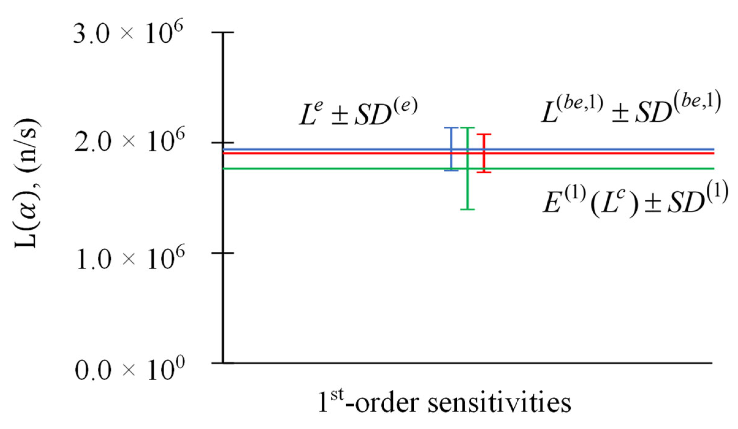
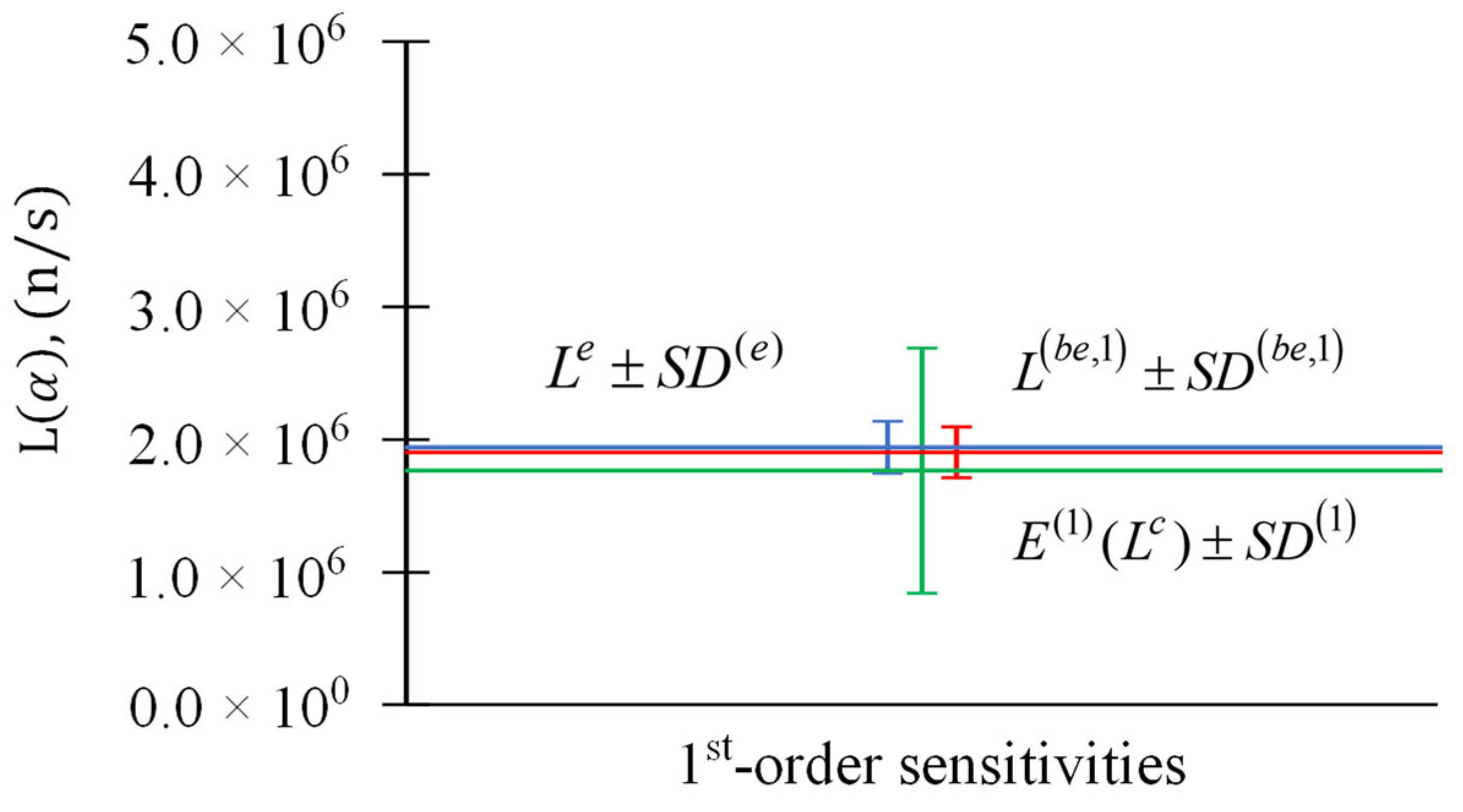
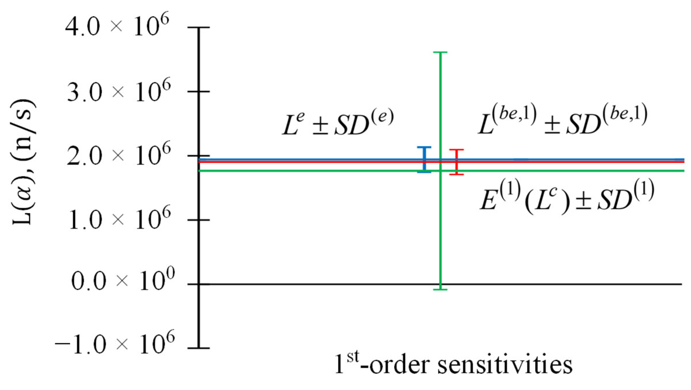
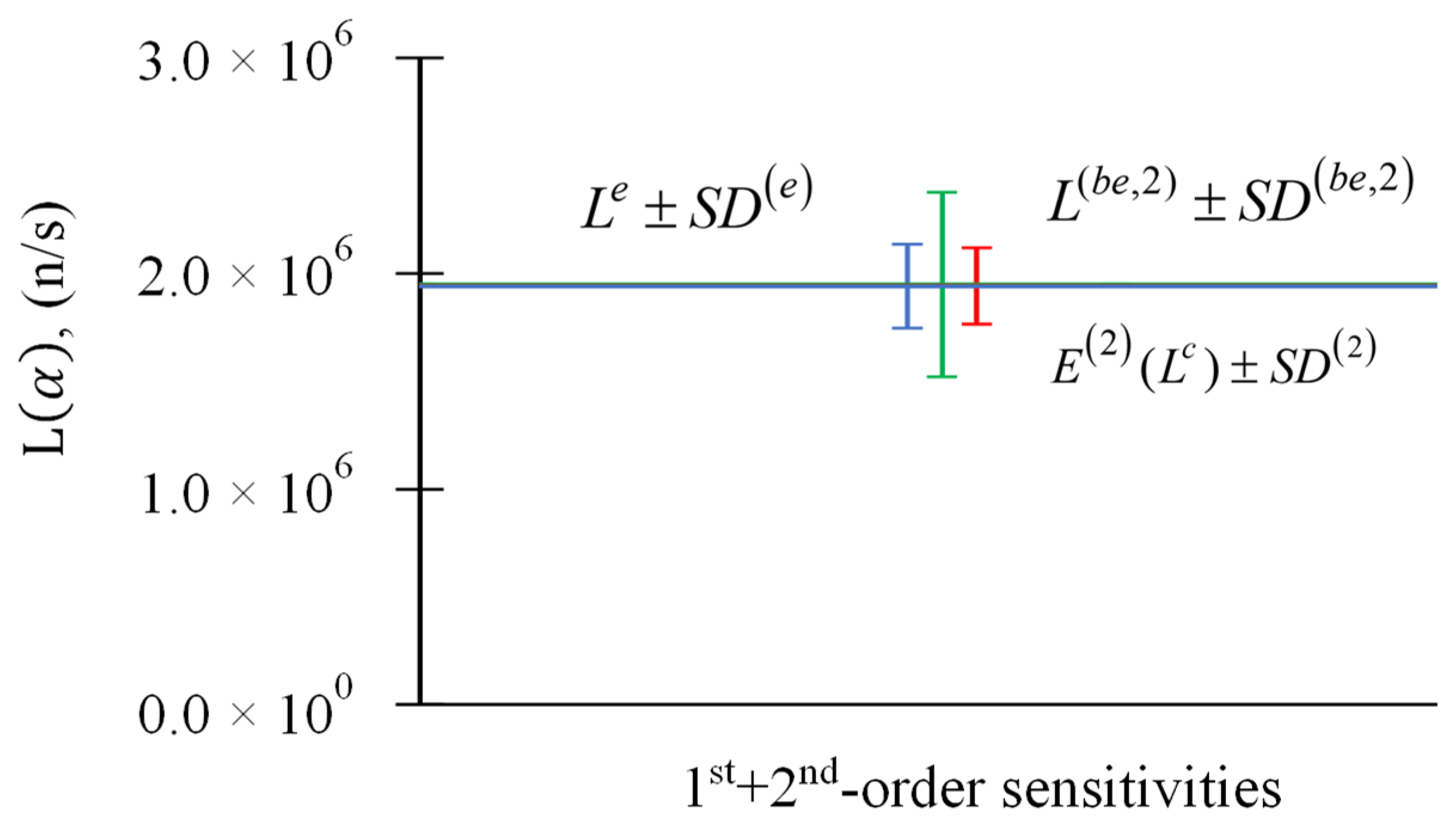
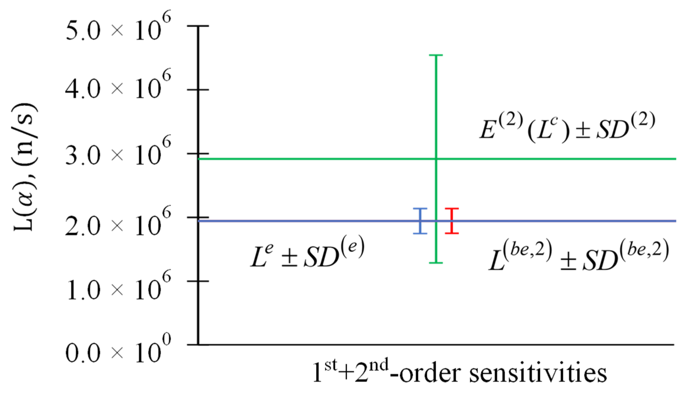
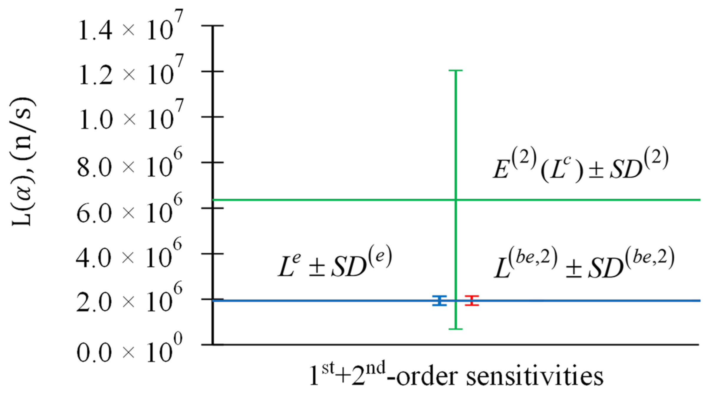
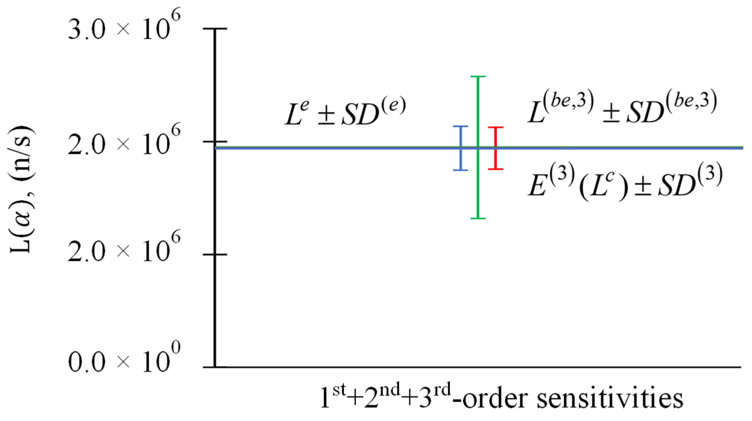
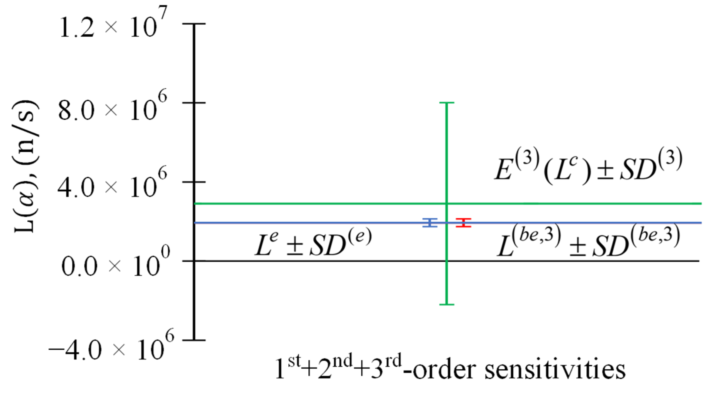
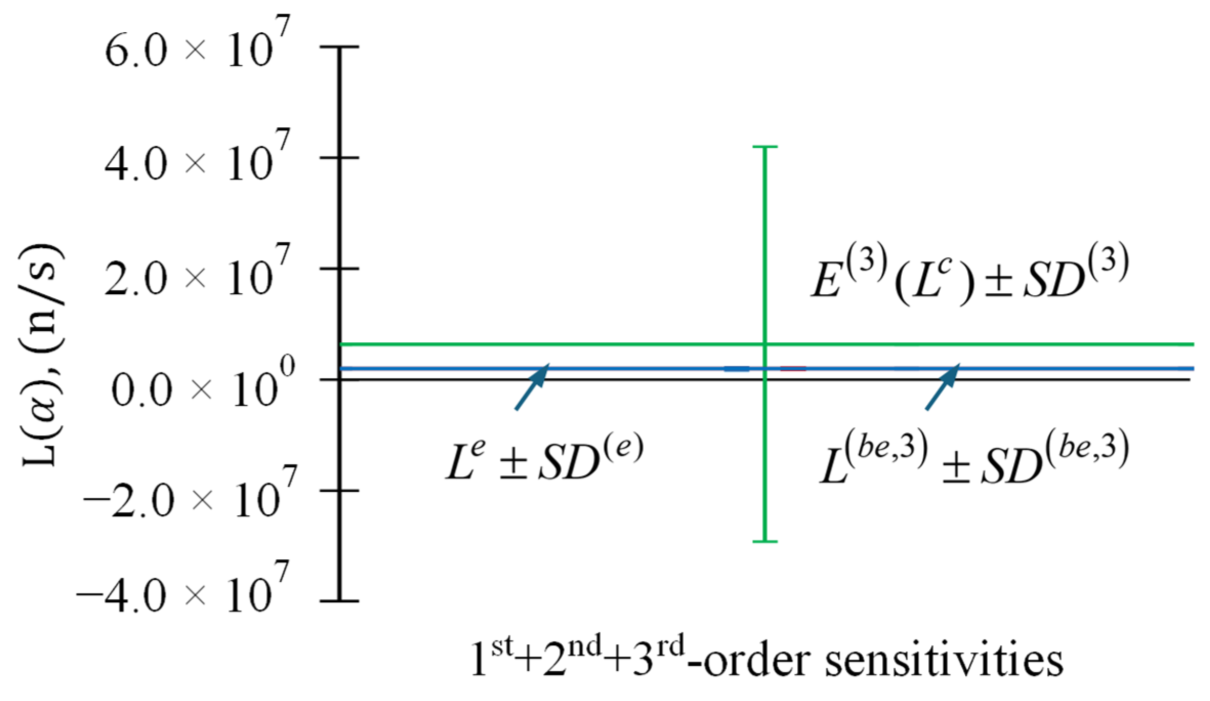
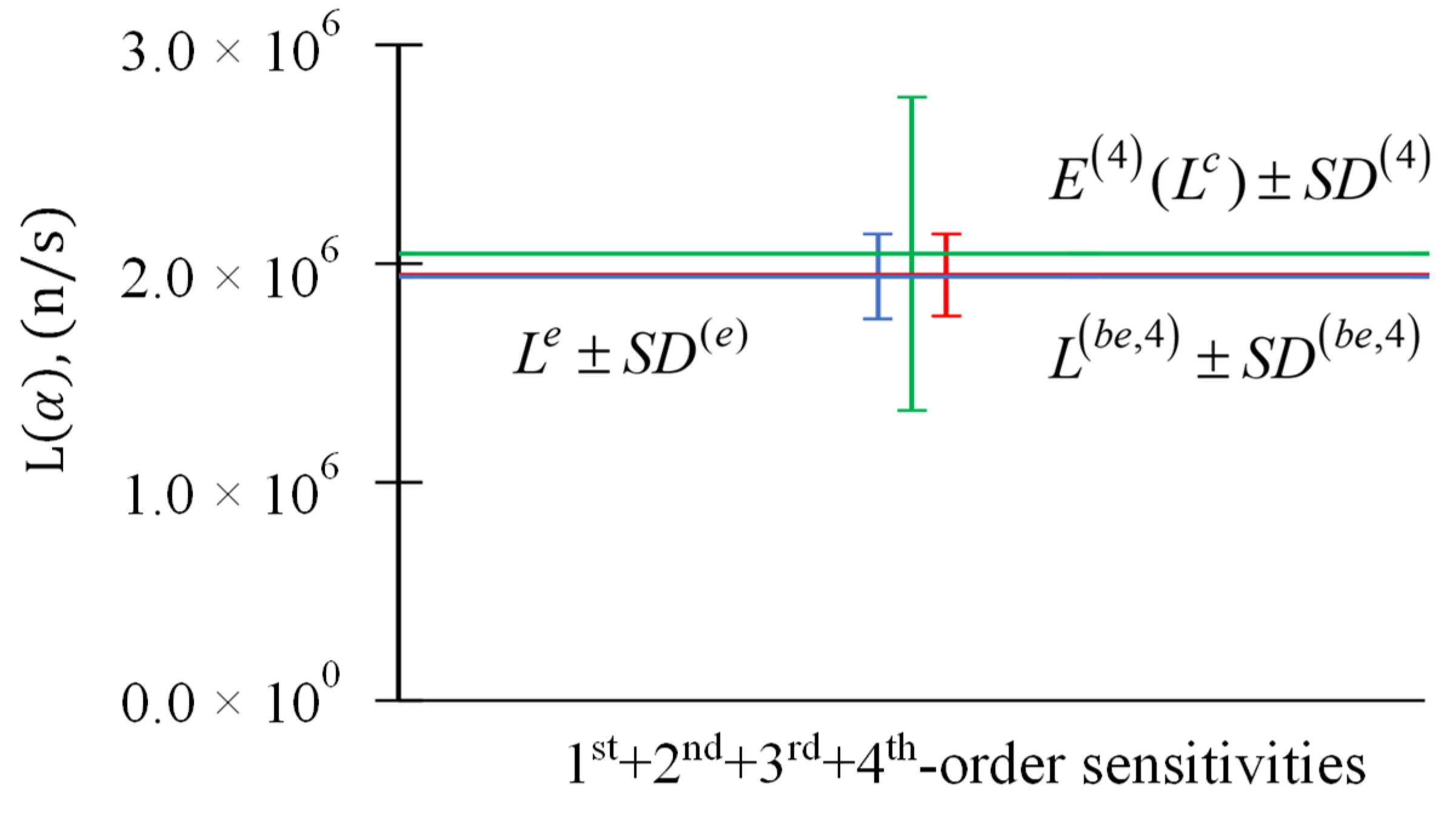
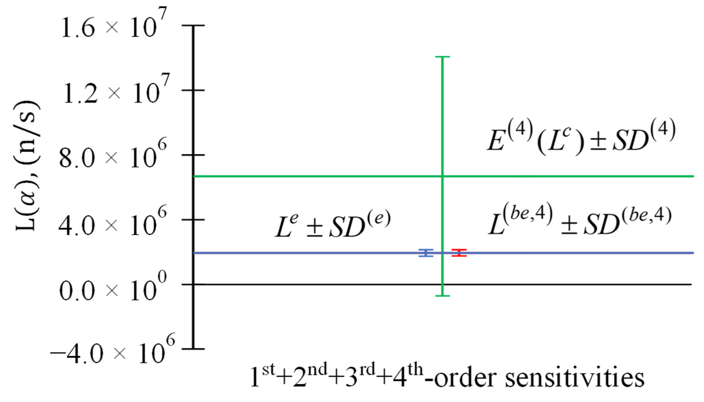
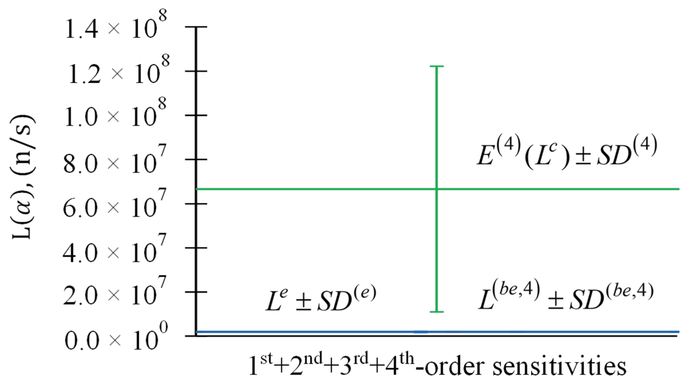
) are illustrated in Figure 1, Figure 2, Figure 3 and Figure 4, below, when considering that the parameters have been measured precisely, having uniform relative standard deviations of 2%. The results presented in Figure 1 include only the first-order sensitivities of the leakage response with respect to the model parameters (total microscopic group cross sections). The results presented in Figure 2 include the first- and second-order sensitivities. The results depicted in Figure 3 include first- through third-order sensitivities, while the results depicted in Figure 4 include all sensitivities up to (and including) fourth-order. The numerical values of the results depicted in Figure 1, Figure 2, Figure 3 and Figure 4 are tabulated in Table 1. The results depicted in Figure 1, Figure 2, Figure 3 and Figure 4 are tabulated numerically in Table 1, below.

The results presented in Figure 1, Figure 2, Figure 3 and Figure 4 and Table 1 indicate that the application of the BERRU-PM methodology yields a best-estimate value for the predicted leakage response which is in-between the experimentally measured and computed values of this response (but closer to the more precisely known experimental value), with an accompanying predicted standard deviation which is smaller than either the measured or the computed standard deviations. Since the standard deviations (of 2%) for the model parameters are within the radius of convergence of the Taylor-series that represents the computed response in terms of parameter deviations, the contributions stemming from the higher-order sensitivities are expected to diminish with increasing order. This expectation is confirmed by the results shown in Figure 1, Figure 2, Figure 3 and Figure 4 and Table 1, which indicate that the impact of the second- and higher-order sensitivities on the best-estimate predicted leakage response and accompanying predicted standard deviation are small.

4.1.2.“. Medium Precision” Parameters, Having Uniform Relative Standard Deviations $S D = 5 %$

Figure 5, Figure 6, Figure 7 and Figure 8, below, depict the results of applying Eqs. (17)‒(33) to the PERP benchmark, in conjunction with the same experimental information as mentioned above (i.e.,

L^{e} = 1.94 \times 10^{6}

with

S D^{(e)} = 10 %

), but considering that the parameters have been measured with a precision (qualified as being “medium”) which is typical of cross section measurements, having uniform relative standard deviations of 5%. The results presented in Figure 5 include only the first-order sensitivities of the leakage response with respect to the model parameters (total microscopic group cross sections). The results presented in Figure 6 include the first- and second-order sensitivities. The results depicted in Figure 7 include first- through third-order sensitivities, while the results depicted in Figure 8 include all sensitivities up to (and including) fourth-order. The numerical values of the results depicted in Figure 5, Figure 6, Figure 7 and Figure 8 are tabulated in Table 2.

As indicated by the results shown in Figure 5, Figure 6, Figure 7 and Figure 8 and Table 2, the contributions stemming from the higher-order sensitivities to the quantities

E^{(i)} (L^{c}) \pm S D^{(i)}

increase with increasing order of sensitivities retained, thus confirming the expectation that the parameter standard deviations are sufficiently large to cause divergence of the Taylor-series that is used to represent the expected value and the standard deviation of the computed response in terms of parameter standard deviations. Nevertheless, the application of the BERRU-PM methodology yields a best-estimate value for the predicted leakage response which falls in-between the experimentally measured and computed values of this response (but closer to the more precisely known experimental value), with an accompanying predicted standard deviation which is smaller than either the measured or the computed standard deviations. These results indicate that the application of the 4th-BERRU-PM methodology can produce physically useful/meaningful results even when the Taylor-series expansion of the response in terms of parameter standard deviations diverges slightly.

4.1.3.“. Low precision” parameters, having uniform relative standard deviations $S D = 10 %$

Figure 9, Figure 10, Figure 11 and Figure 12, below, depict the results of applying Eqs. (17)‒(33) to the PERP benchmark, in conjunction with the same experimental information as mentioned above (i.e.,

L^{e} = 1.94 \times 10^{6}

with

S D^{(e)} = 10 %

), but considering that the parameters have been measured with low precision, having uniform relative standard deviations of 10%. The results presented in Figure 9 include only the first-order sensitivities of the leakage response with respect to the model parameters (total microscopic group cross sections). The results presented in Figure 10 include the first- and second-order sensitivities. The results depicted in Figure 11 include first- through third-order sensitivities, while the results depicted in Figure 12 include all sensitivities up to (and including) fourth-order. The numerical values of the results depicted in Figure 9, Figure 10, Figure 11 and Figure 12 are tabulated in Table 3.

The results presented in Figure 9, Figure 10, Figure 11 and Figure 12 and Table 3 confirm the expectation that parameter standard deviations of 10% cause massive divergence of the Taylor-series used to represent the expected value and standard deviation of the computed response in terms of parameter standard deviations. Nevertheless, as indicated by the last column in Table 3, the application of the BERRU-PM methodology yields a best-estimate value and reduced predicted standard deviation for the predicted leakage response which is close to the more precisely-known experimental values. These results indicate that the application of the 4th-BERRU-PM methodology predicts results that remain physically useful/meaningful even when the parameters uncertainties (measured by the respective standard deviations) are sufficiently large to cause indisputable divergence of the Taylor-series expansion of the response in terms of parameter deviations. However, since parameter standard deviations of 5% already cause the Taylor-series of the response, cf. Eq. (16), to diverge, and since microscopic cross sections are generally known with a precision of 5% or better, only parameter standard deviations of 2% and 5% will henceforth be considered for the subsequent illustrative applications of the 4th-BERRU-PM methodology to the PERP benchmark.

4.2. Effects of Sensitivities and Parameter Standard Deviations on the Predicted Values of the Best-Estimate Correlations between the Leakage Response and the Most Important Parameters

The components of the vectors

C_{α r}^{(b e, i)}

i = 1, ..., 4

, of best-estimate correlations among the benchmark’s leakage response and parameters are computed using the expression provided in Eq. (35). The impact of the parameters’ precision and of the sensitivities of various orders will be illustrated below in Subsection 4.2.l (for “high precision parameters” having uniform relative standard deviations of 2%) and, respectively, Subsection 4.2.2 (for “medium precision parameters” having uniform relative standard deviations of 5%). All of the numerical results presented in this Section for the components of the vectors

C_{α r}^{(b e, i)}

i = 1, ..., 4

, are in units of “[parameter units] x [response units]”, i.e., [barns x neutrons/sec], where 1 barn=10-24 cm2.

4.2.1. “High Precision” Parameters, Having Uniform Relative Standard Deviations $S D = 2 %$

When only the first- and second-order sensitivities are considered, the numerical results for the components of the vectors

C_{α r}^{(c, i)}

i = 1, 2

, are computed using the expression provided in Eq. (36). For the PERP benchmark, each of the vectors

C_{α r}^{(b e, 1)}

and

C_{α r}^{(b e, 2)}

has 180 components, as there are 180 parameters corresponding to the microscopic total cross sections for all 6 isotopes in the benchmark [4]. When only the 1st-order sensitivities are considered, the numerical results for the components of the vector

C_{α r}^{(b e, 1)}

for the top 10 parameters (ranked in the order of the magnitude of their 1st-order relative sensitivities) are presented in Table 4. When both the 1st-order and 2nd-order sensitivities are considered, the numerical results for the components of the vector

C_{α r}^{(b e, 2)}

for the top 10 parameters (also ranked in the order of the magnitude of their 1st-order relative sensitivities) are presented in Table 5.

Comparing the results presented in Table 4 and Table 5 indicates the following conclusions:

(i): Even though the original correlations $C_{α r}^{(c, 1)} = C_{α r}^{(c, 2)}$ between the model parameters and the computed leakage response were negative, the best estimate correlations are positive, i.e., the components of $C_{α r}^{(b e, 1)}$ and $C_{α r}^{(b e, 2)}$ are all positive.
(ii): The absolute values of the components of $C_{α r}^{(b e, 1)}$ and $C_{α r}^{(b e, 2)}$ are all considerably smaller than the absolute values of the original correlations $C_{α r}^{(c, 1)} = C_{α r}^{(c, 2)}$ .
(iii): The values of the components of $C_{α r}^{(b e, 1)}$ are larger than the corresponding components of $C_{α r}^{(b e, 2)}$ , which indicates that the inclusion of the 2nd-order sensitivities reduces the best-estimate correlations between the best-estimate parameters and the predicted best-estimate leakage response.

When the third- and, respectively, fourth-order sensitivities are also included in addition to the first- and second-order sensitivities, the numerical results for the components of the vectors

C_{α r}^{(c, i)}

i = 3, 4

, are computed using the expression provided in Eq. (37). The numerical results thus obtained for the components of the vector

C_{α r}^{(b e, 3)}

and, respectively,

C_{α r}^{(b e, 4)}

, for the top 10 parameters (ranked in the order of the magnitude of their 1st-order relative sensitivities), are presented in Table 6 and Table 7, respectively.

Comparing the results presented in Table 4, Table 5, Table 6 and Table 7 indicates the following conclusions, in addition to the conclusions drawn from the results presented in Table 4 and Table 5:

(i): All of the components of the original correlations $C_{α r}^{(c, 3)} = C_{α r}^{(c, 4)}$ and $C_{α r}^{(c, 1)} = C_{α r}^{(c, 2)}$ between the model parameters and the computed leakage response are negative. Furthermore, including the 3rd- and 4th-order sensitivities causes the absolute values of the components of $C_{α r}^{(c, 3)} = C_{α r}^{(c, 4)}$ to be larger than the corresponding components of the vector $C_{α r}^{(c, 1)} = C_{α r}^{(c, 2)}$ .
(ii): The components of the vectors $C_{α r}^{(b e, i)}$ , $i = 1, ..., 4$ , representing the best-estimate correlations among the benchmark’s best-estimate leakage response and best-estimate parameters, are all positive.
(iii): The values of the components of $C_{α r}^{(b e, 1)}$ are larger than the corresponding components of $C_{α r}^{(b e, 2)}$ , which in turn are larger than the components of $C_{α r}^{(b e, 3)}$ , which in turn are larger than the components of $C_{α r}^{(b e, 4)}$ . This sequence of inequalities indicates that the inclusion of the successively higher-order sensitivities reduces successively the corresponding best-estimate correlations between the best-estimate parameters and the predicted best-estimate leakage response.

4.2.2. “Medium Precision” Parameters, Having Uniform Relative Standard Deviations $S D = 5 %$

When the parameters are considered to be characterized by uniform relative standard deviations of 5%, the numerical results obtained for the components of the vectors

C_{α r}^{(b e, i)}

i = 1, ..., 4

, of best-estimate correlations among the benchmark’s best-estimate leakage response and the top 10 parameters (ranked in the order of the magnitude of their 1st-order relative sensitivities), are presented in below in Table 8, Table 9, Table 10 and Table 11, respectively. As before, when only the first- and second-order sensitivities are considered, the numerical results for the components of the vectors

C_{α r}^{(c, i)}

i = 1, 2

, are computed using the expression provided in Eq. (36). Similarly, when the third- and fourth-order sensitivities are also included, the numerical results for the components of the vectors

C_{α r}^{(c, i)}

i = 3, 4

, are computed using the expression provided in Eq. (37).

Comparing the results presented in Table 8, Table 9, Table 10 and Table 11 with the corresponding results presented in Table 4, Table 5, Table 6 and Table 7 reveals that the larger parameters standard deviations (

S D = 5 %

) accentuate the characteristics displayed by the corresponding results for the smaller parameter standard deviations (

S D = 2 %

), as follows:

(i): Comparing the results in Table 8 with the results presented in Table 4 reveals that the components of the correlations $C_{α r}^{(c, 1)}$ for $S D = 5 %$ are considerably larger in absolute values than the components of the correlations $C_{α r}^{(c, 1)}$ for $S D = 2 %$ . Conversely (and consequently), the components of the best-estimate correlations $C_{α r}^{(b e, 1)}$ for $S D = 5 %$ are considerably larger in absolute values than the components of the correlations $C_{α r}^{(b e, 1)}$ for $S D = 2 %$ . Similar conclusion can be drawn by: (a) comparing the results in Table 9 with the results presented in Table 5; (b) comparing the results in Table 10 with the results presented in Table 6; and (c) comparing the results in Table 11 with the results presented in Table 7.
(ii): All of the conclusions previously drawn from the results obtained for the smaller parameter standard deviations ( $S D = 2 %$ ) also hold for the larger parameters standard deviations ( $S D = 5 %$ ), so they will not be repeated here, other than to note that these conclusions are even more evident/accentuated by the contrast between the original values for the correlations $C_{α r}^{(c, i)}$ (between the model parameters and computed leakage response) and the predicted best-estimate values for the posterior best-estimate correlations, $C_{α r}^{(b e, i)}$ , between the calibrated best-estimate parameters and the best-estimate predicted response. In particular, the starkest contrasts among the original and predicted posterior values for the parameter-response correlations are evidenced by the results presented in Table 11: the original components of the vector $C_{α r}^{(c, 4)}$ all have large negative values of the order of $O (10^{5} - 10^{7})$ , while the posterior best-estimate correlations $C_{α r}^{(b e, 4)}$ have positive values of the order of $O (10 - 10^{3})$ .

The overall conclusion that follows from the results presented in Table 4, Table 5, Table 6, Table 7, Table 8, Table 9, Table 10 and Table 11 is that the larger the parameter standard deviation and the higher the order of retained sensitivities, the larger the negative values of the original correlations among the model parameters and the leakage response, and the smaller the positive values of the best-estimate predicted posterior correlations among the best-estimate posterior calibrated model parameters and the predicted posterior leakage response.

4.3. Effects of Sensitivities and Parameter Standard Deviations on the Predicted Values of the Best-Estimate Calibrated Model Parameters

The best-estimate predicted values of the calibrated model parameters,

α^{(b e, i)}

i = 1, 2, 3, 4

, are computed by using Eq. (40). All of the numerical results presented in this Section for the best-estimate predicted calibrated parameter values are in units of “barn”, where 1 barn=10-24 cm2. Table 12 presents the results for the best-estimate predicted values for the top 10 calibrated model parameters (ranked in the order of the magnitude of their 1st-order relative sensitivities) for parameters that are measured with “high precision,” having uniform relative standard deviations

S D = 2 %

. Table 13 presents the results for the best-estimate predicted values for the top 10 calibrated model parameters (ranked in the order of the magnitude of their 1st-order relative sensitivities) for parameters that are measured with “medium precision,” having uniform relative standard deviations

S D = 5 %

. For all of the results presented in these Tables, the nominal value of the measured response is

L^{e} = 1.94 \times 10^{6}

n/s, with a measured relative standard deviation

S D^{(e)} = 10 %

. The results presented in these Tables indicate that the calibration (i.e., adjustment) of each of the respective parameter’s nominal value is negligeable for the realistic values (2-5%) considered for the relative standard deviations for the parameters.

4.4. Effects of Sensitivities and Parameter Standard Deviations on the Predicted Values of the Components of the Covariance Matrix of Predicted Model Parameters

The components of the predicted posterior covariance matrix

C_{α α}^{(b e, i)}

i = 1, 2, 3, 4

, of the best-estimate calibrated parameters are computed by using Eq. (42). All of the numerical results presented in this Section for the components of the best-estimate parameter covariance matrices

C_{α α}^{(b e, i)}

i = 1, ..., 4

, are in units of “

{[b a r n]}^{2}

,” i.e.,

{[10^{- 24} c m^{2}]}^{2}

. As before, all of the results presented in this Section were obtained by considering that the nominal value of the measured response is

L^{e} = 1.94 \times 10^{6}

n/s, with a measured relative standard deviation

S D^{(e)} = 10 %

The diagonal matrix of apriori variances for the top 10 model parameters (ranked in the order of the magnitude of their 1st-order relative sensitivities), which are considered to be uncorrelated, normally distributed, and having uniform relative standard deviations

S D = 2 %

, is presented in Table 14, below. Table 15, Table 16, Table 17 and Table 18, below, present the results for the best-estimate predicted values for the components of the posterior matrices

C_{α α}^{(b e, i)}

i = 1, 2, 3, 4

The results presented in these Tables indicate that the variance of each of the calibrated predicted parameters has been significantly reduced by comparison to its original value. However, this reduction is not monotonic but oscillates with decreasing amplitudes as sensitivities of increasingly higher-order are considered. Furthermore, the originally uncorrelated parameters have become negatively correlated after the application of the 4th-BERRU-PM methodology. The impact of sensitivities higher than first-order is small.

The results for the top 10 model parameters (ranked in the order of the magnitude of their 1st-order relative sensitivities), which are considered to be uncorrelated, normally distributed, and having uniform relative standard deviations

S D = 5 %

, are presented in Table 19, Table 20, Table 21, Table 22 and Table 23, below. Table 19 presents the diagonal matrix of apriori parameter variances. Table 20, Table 21, Table 22 and Table 23 present the results for the predicted values for the components of the posterior matrices

C_{α α}^{(b e, i)}

i = 1, 2, 3, 4

The results presented above in Table 20, Table 21, Table 22 and Table 23 are similar to the results presented in Table 15, Table 16, Table 17 and Table 18, indicating that: (i) the variance of each of the calibrated predicted parameters is significantly reduced by comparison to its original value; this reduction is not monotonic but oscillates with decreasing amplitudes as sensitivities of increasingly higher-order are considered.; (ii) the originally uncorrelated parameters have become negatively correlated after the application of the 4th-BERRU-PM methodology; and (iii) the impact of sensitivities higher than first-order is small.

Recall that the Taylor-series expansion provided in Eq. (16) is divergent for parameter standard deviations of 5% and larger. Nevertheless, it is of interest to show that the application of the 4th-BERRU-PM methodology reduces the standard deviations of the predicted calibrated parameters even in such rather extreme situations, even if just the first- and second-order sensitivities are considered. In this vein, Table 24, Table 25 and Table 26 present the results for the top 10 model parameters (ranked in the order of the magnitude of their 1st-order relative sensitivities), which are considered to be uncorrelated, normally distributed, and having uniform relative standard deviations

S D = 10 %

. Table 24 presents the diagonal matrix of apriori parameter variances. Table 25 and Table 26 present the results for the predicted values for the components of the posterior matrices

C_{α α}^{(b e, i)}

i = 1, 2

. Remarkably, the results presented in these Tables are similar to the results presented in Table 15, Table 16, Table 17 and Table 18 (which were obtained for small parameter standard deviations, of 2%), thus indicating that: (i) the variance of each of the calibrated predicted parameters is significantly reduced by comparison to its original value; this reduction is not monotonic but oscillates with decreasing amplitudes as sensitivities of increasingly higher-order are considered; (ii) the originally uncorrelated parameters have become negatively correlated after the application of the 4th-BERRU-PM methodology.

4.5. Effects of Sensitivities and Parameter Standard Deviations on the Predicted Skewness of the Predicted Leakage Response and, respectively, Calibrated Model Parameters

The most important triple-correlation is the skewness of each individual best-estimate predicted response and calibrated parameters. The skewness of the predicted best-estimate leakage response, denoted as

S k e w^{(b e, i)} (L^{(b e, i)})

, where the index “i" denotes the highest-order of sensitivities retained in the respective computation, is computed using the expression below:

S k e w^{(b e, i)} (L^{(b e, i)}) = μ_{3}^{(b e, i)} (L^{(b e, i)}) {[S D (L^{(b e, i)})]}^{- 3}, i = 1, 2, 3, 4.

(73)

where the expression of the triple-correlation

μ_{3}^{(b e, i)} (L^{(b e, i)})

is provided in Eq. (45), while the expression of the standard deviation

S D (L^{(b e, i)})

is provided in one of Eqs. (30)‒(33), depending on the value of the index “i".

Similarly, the skewness of a predicted best-estimate calibrated parameter

α_{k}^{(b e, i)}

k = 1, ..., T P,

will be denoted as

S k e w^{(b e, i)} (α_{k}^{(b e, i)})

, where the index “i" denotes the highest-order of sensitivities retained in the respective computation, and is computed using the expression below:

S k e w^{(b e, i)} (α_{k}^{(b e, i)}) = μ_{3}^{(b e, i)} (α_{k}^{(b e, i)}) {[S D (α_{k}^{(b e, i)})]}^{- 3}, i = 1, 2, 3, 4.

(74)

In Eq. (74), the expression of the triple-correlation

μ_{3}^{(b e, i)} (α_{k}^{(b e, i)})

is provided in Eq. (57), while the standard deviation

S D (α_{k}^{(b e, i)})

is the square-root of the respective diagonal element of

C_{α α}^{(b e, i)}

, which is obtained using the expression provided in Eq. (42).

The numerical results obtained for the skewness

S k e w^{(b e, i)} (L^{(b e, i)})

of the predicted best-estimate leakage response, and for the skewness

S k e w^{(b e, i)} (α_{k}^{(b e, i)})

for each of the three most important predicted calibrated model parameters are presented below in Table 27 and Table 28, respectively.

The results presented in Table 27 are for uniform relative standard deviations of 2% for the model parameters; recall that the Taylor-series expansion of the computed response in terms of parameter deviations provided in Eq. (16) is convergent for such small standard deviations. Recall that the measurements were considered to be normally distributed (thus having zero skewness); furthermore, the contribution of the initial skewness of the computed responses enters in the expression of the higher-order term

p_{1} (r_{s}^{(0)}, α_{s}^{(0)})

in Eq. (44), which was neglected by comparison to the other terms in this equation. Thus, the skewness of the measured response and the skewness of the computed responses do not influence the predicted skewness, within the second-order approximation inherent in the expression of the predicted skewness. When only the first-order sensitivities are considered, the small positive number for the predicted skewness in Table 27 indicates that the MaxEnt distribution of the predicted best-estimate leakage response is slightly tilted to the right of the distribution’s mean value. However, when the second- and higher-order sensitivities are also considered, the MaxEnt distribution of the predicted best-estimate leakage response becomes tilted just slightly to the left of the distribution’s mean value, but the respective tilt is negligibly small. These results indicate that results based exclusively on first-order sensitivities are unreliable. It is therefore paramount to at least consider the second-order sensitivities, in addition to the first-order ones. The above conclusion holds both for the predicted leakage response and for the calibrated predicted parameters.

The results presented in Table 28 for uniform parameter standard deviations of 5% indicate that the conclusions drawn from the results in Table 27 also hold for these larger standard deviations, which are just outside the convergence radius of the Taylor-series in Eq. (16).

4.6. Effects of Sensitivities and Parameter Standard Deviations on the Predicted Kurtosis of the Predicted Leakage Response and, respectively, Calibrated Model Parameters

The most important quadruple-correlations are the individual kurtoses of the best-estimate predicted response and calibrated parameters. The kurtosis of the predicted best-estimate leakage response, denoted as

K u r t^{(b e, i)} (L^{(b e, i)})

, where the index “i" denotes the highest-order of sensitivities retained in the respective computation, is computed using the expression below:

K u r t^{(b e, i)} (L^{(b e, i)}) = μ_{4}^{(b e, i)} (L^{(b e, i)}) {[S D (L^{(b e, i)})]}^{- 4}, i = 1, 2, 3, 4.

(75)

where the expression of the quadruple-correlation

μ_{4}^{(b e, i)} (L^{(b e, i)})

is provided in Eq. (59), while the expressions of the standard deviation

S D (L^{(b e, i)})

are provided in the corresponding Eqs. (30)‒(33).

Similarly, the kurtosis of a predicted best-estimate calibrated parameter

α_{k}^{(b e, i)}

k = 1, ..., T P,

will be denoted as

K u r t^{(b e, i)} (α_{k}^{(b e, i)})

, where the index “i" denotes the highest-order of sensitivities retained in the respective computation, and is computed using the expression below:

K u r t^{(b e, i)} (α_{k}^{(b e, i)}) = μ_{4}^{(b e, i)} (α_{k}^{(b e, i)}) {[S D (α_{k}^{(b e, i)})]}^{- 4}, i = 1, 2, 3, 4.

(76)

In Eq. (76), the expression of the quadruple-correlation

μ_{4}^{(b e, i)} (α_{k}^{(b e, i)})

is provided in Eq. (68) while the standard deviation

S D (α_{k}^{(b e, i)})

is the square-root of the respective diagonal element of

C_{α α}^{(b e, i)}

, which is obtained using the expression provided in Eq. (42).

The numerical results obtained for the kurtosis

K u r t^{(b e, i)} (L^{(b e, i)})

of the predicted best-estimate leakage response, and for the kurtosis

K u r t^{(b e, i)} (α_{k}^{(b e, i)})

, for each of the three most important calibrated model parameters, are presented in Table 29 and Table 30, below.

The results presented in Table 29 are for uniform relative standard deviations of 2% for the model parameters; recall that the Taylor-series expansion of the computed response in terms of parameter deviations provided in Eq. (16) is convergent for such small standard deviations. When only the first-order sensitivities are considered, the kurtosis of the MaxEnt distribution of the predicted best-estimate leakage response is somewhat “more peaked” than the initial normal distribution. However, when the second- and higher-order sensitivities are also considered, the MaxEnt distribution of the predicted best-estimate leakage response converges to the normal distribution (for which “kurtosis = 3.00”). The same trend is also observed for the most important parameters: recall that the parameters were considered to have initially been normally distributed and uncorrelated, which implies that the distribution of each parameter initially had the value “initial parameter kurtosis = 3.” The MaxEnt distribution of the best-estimate calibrated parameters also remains around the value (=3) of the corresponding normal distribution.

The results presented in Table 30 for uniform parameter standard deviations of 5% indicate that the conclusions drawn from the results in Table 29 also hold for these larger standard deviations, which are just outside the convergence radius of the Taylor-series in Eq. (16).

5. Concluding Discussion

This work has reviewed the fourth-order “data assimilation (DA)” and “model calibration (MC)” outputs of the 4th-BERRU-PM methodology, which encompass the fourth-order MaxEnt posterior distribution of experimentally measured and computed model responses and parameters, in the combined phase-space of model responses and parameters, as well as the first-order through fourth-order moments (predicted mean values, covariances, third- and fourth-order correlations, including skewness and kurtosis of responses and calibrated parameters) of this posterior distribution. The mathematical expressions for these moments were applied to obtain specialized numerical results for the PERP reactor physics benchmark [2], which is modeled by the neutron transport equation comprising 21,976 uncertain model parameters and is therefore representative of “large-scale” computational models of energy systems. The result (“response”) of interest for the PERP benchmark is the leakage of neutrons through the outer surface of this spherical benchmark, which can be computed numerically and measured experimentally. The fourth-order “sensitivity analysis (SA)” and “uncertainty quantification (UQ)” which are used as “input” into the 4th-BERRU-PM methodology, were reviewed in Part 1 [4], which also presented numerical illustrations using the PERP benchmark.

This work has also quantified the impact of combinations of sensitivities of increasingly higher order and various values for the standard deviations of the model’s parameters. The impact of the high-order sensitivities was quantified for “high-precision” parameters (2% standard deviations) and “medium-precision” parameters (5% standard deviations). Analyzing the best-estimate results with reduced uncertainties for the 1st- through 4th-order moments (mean values, covariance, skewness, and kurtosis) produced by the 4th-BERRU-PM methodology for the PERP benchmark has indicated that, even for systems modeled by linear equations (such as the PERP benchmark), retaining only first-order sensitivities is insufficient for reliable predictive modeling (including SA, UQ, DA, MC). At least second-order sensitivities should be retained in order to obtain reliable predictions. For large parameter uncertainties, it is also advisable to apply the 4th-BERRU-PM methodology sequentially and repeatedly, using new experimental information in conjunction with the calibrated model parameters from the previous application of the 4th-BERRU-PM methodology.

Author Contributions

Conceptualization: D.G.C.; Investigation: R.F.; Writing—original draft: D.G.C.; Writing—review & editing: R.F. and D.G.C. All authors have read and agreed to the published version of the manuscript.

Funding

This research received no external funding.

Data Availability Statement

All data are available in the main text.

Conflicts of Interest

The authors declare no conflict of interest.

References

Cacuci, D.G. Fourth-Order Predictive Modelling: II. 4th-BERRU-PM Methodology for Combining Measurements with Computations to Obtain Best-Estimate Results with Reduced Uncertainties. Am. J. Comp. Math. 2023, 13, 439–475. [Google Scholar] [CrossRef]
Valentine, T.E. Polyethylene-Reflected Plutonium Metal Sphere Subcritical Noise Measurements. SUB-PU-METMIXED-001, International Handbook of Evaluated Criticality Safety Benchmark Experiments; NEA/NSC/DOC(95)03/I-IX; Organization for Economic Co-Operation and Development; Nuclear Energy Agency: Paris, France, 2006.
Jaynes, E.T. Information Theory and Statistical Mechanics. Phys. Rev. 1957, 106, 620. [Google Scholar] [CrossRef]
Cacuci, D.G.; Fang, R. Review of Fourth-Order Maximum Entropy Based Predictive Modelling and Illustrative Application to a Nuclear Reactor Benchmark: I. Typical High-Order Sensitivity and Uncertainty Analysis. Energies, 2024, submitted.
Cacuci, D.G. The nth-Order Comprehensive Adjoint Sensitivity Analysis Methodology: Overcoming the Curse of Dimensionality. Volume I: Linear Systems. Springer Nature Switzerland, Cham, Switzerland, 2022. [CrossRef]
Cacuci, D.G. The nth-Order Comprehensive Adjoint Sensitivity Analysis Methodology (nth-CASAM): Overcoming the Curse of Dimensionality in Sensitivity and Uncertainty Analysis, Volume III: Nonlinear Systems. Springer Nature Switzerland, Cham, 2023. [CrossRef]
Bellman, R.E. Dynamic programming. Rand Corporation, Princeton University Press, ISBN 978-0-691-07951-6, USA. 1957.
Cacuci, D.G. Second-Order MaxEnt Predictive Modelling Methodology. I: Deterministically Incorporated Computational Model (2nd-BERRU-PMD). Am. J. Comp. Math. 2013, 13, 236–266. [Google Scholar] [CrossRef]
Cacuci, D.G. Second-Order MaxEnt Predictive Modelling Methodology. II: Probabilistically Incorporated Computational Model (2nd-BERRU-PMP). Am. J. Comp. Math. 2023, 13, 267–294. [Google Scholar] [CrossRef]
SCALE: a modular code system for performing standardized computer analyses for licensing evaluation, ORNL/TM 2005/39, Version 6, Oak Ridge National Laboratory, Oak Ridge, Tennessee, USA, 2009.
Venard, C.; Santamarina, A.; Leclainche, A.; Mournier, C. The R.I.B. Tool for the determination of computational bias and associated uncertainty in the CRISTAL criticality safety package. Proceedings of ANS Nuclear Criticality Safety Division Topical Meeting (NCSD 2009), Richland, Washington, USA, 2009.
Rabier, F. Overview of global data assimilation developments in numerical weather-prediction centers. Q. J. R. Meteorol. Soc. 2005, 131, 3215. [Google Scholar] [CrossRef]
Lewis, J.M.; Lakshmivarahan, S.; Dhall, S.K. Dynamic Data Assimilation: A Least Square Approach. Cambridge University Press, Cambridge, UK, 2006.
Lahoz, W.; Khattatov, B.; Ménard, R. Eds. Data Assimilation: Making Sense of Observations, Springer Verlag, Heidelberg, Germany, 2010.
Práger, T.; Kelemen, F.D. Adjoint methods and their application in earth sciences. Chapter 4, Part A, pp 203-275, in Faragó, I.; Havasi, Á.; Zlatev, Z. (Eds.) Advanced Numerical Methods for Complex Environmental Models: Needs and Availability, Bentham Science Publishers, Bussum, The Netherlands, 2013.
Cacuci, D.G.; Navon, M.I.; Ionescu-Bujor, M. Computational Methods for Data Evaluation and Assimilation. Chapman & Hall/CRC, Boca Raton, USA, 2014.

Figure 1. Parameter relative standard deviations

S D = 2 %

: (i) experimentally measured response and its standard deviation

L^{e} \pm S D^{(e)}

(blue); (ii) expected value of computed response and its standard deviation

E^{(1)} (L^{c}) \pm S D^{(1)}

(green) including only first-order sensitivities; (iii) best-estimate predicted leakage response and its predicted best-estimate standard deviation

L^{(b e, 1)} \pm S D^{(b e, 1)}

(red) including only first-order sensitivities.

Figure 1. Parameter relative standard deviations

S D = 2 %

: (i) experimentally measured response and its standard deviation

L^{e} \pm S D^{(e)}

(blue); (ii) expected value of computed response and its standard deviation

E^{(1)} (L^{c}) \pm S D^{(1)}

(green) including only first-order sensitivities; (iii) best-estimate predicted leakage response and its predicted best-estimate standard deviation

L^{(b e, 1)} \pm S D^{(b e, 1)}

(red) including only first-order sensitivities.

Figure 2. Parameter relative standard deviations

S D = 2 %

: (i) experimentally measured response and its standard deviation

L^{e} \pm S D^{(e)}

(blue); (ii) expected value of computed response and its standard deviation

E^{(2)} (L^{c}) \pm S D^{(2)}

(green) including first- and second-order sensitivities; (iii) best-estimate predicted leakage response and its predicted best-estimate standard deviation

L^{(b e, 2)} \pm S D^{(b e, 2)}

(red) including first- and second-order sensitivities.

Figure 2. Parameter relative standard deviations

S D = 2 %

: (i) experimentally measured response and its standard deviation

L^{e} \pm S D^{(e)}

(blue); (ii) expected value of computed response and its standard deviation

E^{(2)} (L^{c}) \pm S D^{(2)}

(green) including first- and second-order sensitivities; (iii) best-estimate predicted leakage response and its predicted best-estimate standard deviation

L^{(b e, 2)} \pm S D^{(b e, 2)}

(red) including first- and second-order sensitivities.

Figure 3. Parameter relative standard deviations

S D = 2 %

: (i) experimentally measured response and its standard deviation

L^{e} \pm S D^{(e)}

(blue); (ii) expected value of computed response and its standard deviation

E^{(3)} (L^{c}) \pm S D^{(3)}

(green) including first-, second, and third-order sensitivities; (iii) best-estimate predicted leakage response and its predicted best-estimate standard deviation

L^{(b e, 3)} \pm S D^{(b e, 3)}

(red) including first-, second, and third-order sensitivities.

Figure 3. Parameter relative standard deviations

S D = 2 %

: (i) experimentally measured response and its standard deviation

L^{e} \pm S D^{(e)}

(blue); (ii) expected value of computed response and its standard deviation

E^{(3)} (L^{c}) \pm S D^{(3)}

(green) including first-, second, and third-order sensitivities; (iii) best-estimate predicted leakage response and its predicted best-estimate standard deviation

L^{(b e, 3)} \pm S D^{(b e, 3)}

(red) including first-, second, and third-order sensitivities.

Figure 4. Parameter relative standard deviations

S D = 2 %

: (i) experimentally measured response and its standard deviation

L^{e} \pm S D^{(e)}

(blue); (ii) expected value of computed response and its standard deviation

E^{(4)} (L^{c}) \pm S D^{(4)}

(green) including first- through fourth-order sensitivities; (iii) best-estimate predicted leakage response and its predicted best-estimate standard deviation

L^{(b e, 4)} \pm S D^{(b e, 4)}

(red) including first- through fourth-order sensitivities.

Figure 4. Parameter relative standard deviations

S D = 2 %

: (i) experimentally measured response and its standard deviation

L^{e} \pm S D^{(e)}

(blue); (ii) expected value of computed response and its standard deviation

E^{(4)} (L^{c}) \pm S D^{(4)}

(green) including first- through fourth-order sensitivities; (iii) best-estimate predicted leakage response and its predicted best-estimate standard deviation

L^{(b e, 4)} \pm S D^{(b e, 4)}

(red) including first- through fourth-order sensitivities.

Figure 5. Parameter relative standard deviations

S D = 5 %

: (i) experimentally measured response and its standard deviation

L^{e} \pm S D^{(e)}

(blue); (ii) expected value of computed response and its standard deviation

E^{(1)} (L^{c}) \pm S D^{(1)}

(green) including only first-order sensitivities; (iii) best-estimate predicted leakage response and its predicted best-estimate standard deviation

L^{(b e, 1)} \pm S D^{(b e, 1)}

(red) including only first-order sensitivities.

Figure 5. Parameter relative standard deviations

S D = 5 %

: (i) experimentally measured response and its standard deviation

L^{e} \pm S D^{(e)}

(blue); (ii) expected value of computed response and its standard deviation

E^{(1)} (L^{c}) \pm S D^{(1)}

(green) including only first-order sensitivities; (iii) best-estimate predicted leakage response and its predicted best-estimate standard deviation

L^{(b e, 1)} \pm S D^{(b e, 1)}

(red) including only first-order sensitivities.

Figure 6. Parameter relative standard deviations

S D = 5 %

: (i) experimentally measured response and its standard deviation

L^{e} \pm S D^{(e)}

(blue); (ii) expected value of computed response and its standard deviation

E^{(2)} (L^{c}) \pm S D^{(2)}

(green) including first- and second-order sensitivities; (iii) best-estimate predicted leakage response and its predicted best-estimate standard deviation

L^{(b e, 2)} \pm S D^{(b e, 2)}

(red) including first- and second-order sensitivities.

Figure 6. Parameter relative standard deviations

S D = 5 %

: (i) experimentally measured response and its standard deviation

L^{e} \pm S D^{(e)}

(blue); (ii) expected value of computed response and its standard deviation

E^{(2)} (L^{c}) \pm S D^{(2)}

(green) including first- and second-order sensitivities; (iii) best-estimate predicted leakage response and its predicted best-estimate standard deviation

L^{(b e, 2)} \pm S D^{(b e, 2)}

(red) including first- and second-order sensitivities.

Figure 7. Parameter relative standard deviations

S D = 5 %

: (i) experimentally measured response and its standard deviation

L^{e} \pm S D^{(e)}

(blue); (ii) expected value of computed response and its standard deviation

E^{(3)} (L^{c}) \pm S D^{(3)}

(green) including first-, second, and third-order sensitivities; (iii) best-estimate predicted leakage response and its predicted best-estimate standard deviation

L^{(b e, 3)} \pm S D^{(b e, 3)}

(red) including first-, second, and third-order sensitivities.

Figure 7. Parameter relative standard deviations

S D = 5 %

: (i) experimentally measured response and its standard deviation

L^{e} \pm S D^{(e)}

(blue); (ii) expected value of computed response and its standard deviation

E^{(3)} (L^{c}) \pm S D^{(3)}

(green) including first-, second, and third-order sensitivities; (iii) best-estimate predicted leakage response and its predicted best-estimate standard deviation

L^{(b e, 3)} \pm S D^{(b e, 3)}

(red) including first-, second, and third-order sensitivities.

Figure 8. Parameter relative standard deviations

S D = 5 %

: (i) experimentally measured response and its standard deviation

L^{e} \pm S D^{(e)}

(blue); (ii) expected value of computed response and its standard deviation

E^{(4)} (L^{c}) \pm S D^{(4)}

(green) including first- through fourth-order sensitivities; (iii) best-estimate predicted leakage response and its predicted best-estimate standard deviation

L^{(b e, 4)} \pm S D^{(b e, 4)}

(red) including first- through fourth-order sensitivities.

Figure 8. Parameter relative standard deviations

S D = 5 %

: (i) experimentally measured response and its standard deviation

L^{e} \pm S D^{(e)}

(blue); (ii) expected value of computed response and its standard deviation

E^{(4)} (L^{c}) \pm S D^{(4)}

(green) including first- through fourth-order sensitivities; (iii) best-estimate predicted leakage response and its predicted best-estimate standard deviation

L^{(b e, 4)} \pm S D^{(b e, 4)}

(red) including first- through fourth-order sensitivities.

Figure 9. Comparison of

E^{(i)} (L^{c}) \pm S D^{(i)}

(in green),

L^{(b e, i)} \pm S D^{(b e, i)}

(in red), and

L^{e} \pm S D^{(e)}

(in blue), for response measurement for response measurement

L^{e} = 1.94 \times 10^{6}

n/s,

S D^{(e)} = 10 %

, and parameters

S D = 10 %

. Only the 1st-order (

i = 1

) sensitivities are considered.

Figure 9. Comparison of

E^{(i)} (L^{c}) \pm S D^{(i)}

(in green),

L^{(b e, i)} \pm S D^{(b e, i)}

(in red), and

L^{e} \pm S D^{(e)}

(in blue), for response measurement for response measurement

L^{e} = 1.94 \times 10^{6}

n/s,

S D^{(e)} = 10 %

, and parameters

S D = 10 %

. Only the 1st-order (

i = 1

) sensitivities are considered.

Figure 10. Comparison of

E^{(i)} (L^{c}) \pm S D^{(i)}

(in green),

L^{(b e, i)} \pm S D^{(b e, i)}

(in red), and

L^{e} \pm S D^{(e)}

(in blue), for response measurement for response measurement

L^{e} = 1.94 \times 10^{6}

n/s,

S D^{(e)} = 10 %

, and parameters

S D = 10 %

. The 1st + 2nd-order (

i = 2

) sensitivities are included.

Figure 10. Comparison of

E^{(i)} (L^{c}) \pm S D^{(i)}

(in green),

L^{(b e, i)} \pm S D^{(b e, i)}

(in red), and

L^{e} \pm S D^{(e)}

(in blue), for response measurement for response measurement

L^{e} = 1.94 \times 10^{6}

n/s,

S D^{(e)} = 10 %

, and parameters

S D = 10 %

. The 1st + 2nd-order (

i = 2

) sensitivities are included.

Figure 11. Comparison of

E^{(i)} (L^{c}) \pm S D^{(i)}

(in green),

L^{(b e, i)} \pm S D^{(b e, i)}

(in red), and

L^{e} \pm S D^{(e)}

(in blue), for response measurement for response measurement

L^{e} = 1.94 \times 10^{6}

n/s,

S D^{(e)} = 10 %

, and parameters

S D = 10 %

. The 1st + 2nd + 3rd-order (

i = 3

) sensitivities are included.

Figure 11. Comparison of

E^{(i)} (L^{c}) \pm S D^{(i)}

(in green),

L^{(b e, i)} \pm S D^{(b e, i)}

(in red), and

L^{e} \pm S D^{(e)}

(in blue), for response measurement for response measurement

L^{e} = 1.94 \times 10^{6}

n/s,

S D^{(e)} = 10 %

, and parameters

S D = 10 %

. The 1st + 2nd + 3rd-order (

i = 3

) sensitivities are included.

Figure 12. Comparison of

E^{(i)} (L^{c}) \pm S D^{(i)}

(in green),

L^{(b e, i)} \pm S D^{(b e, i)}

(in red), and

L^{e} \pm S D^{(e)}

(in blue), for response measurement for response measurement

L^{e} = 1.94 \times 10^{6}

n/s,

S D^{(e)} = 10 %

, and parameters

S D = 10 %

. The 1st + 2nd + 3rd + 4th-order (

i = 4

) sensitivities are included.

Figure 12. Comparison of

E^{(i)} (L^{c}) \pm S D^{(i)}

(in green),

L^{(b e, i)} \pm S D^{(b e, i)}

(in red), and

L^{e} \pm S D^{(e)}

(in blue), for response measurement for response measurement

L^{e} = 1.94 \times 10^{6}

n/s,

S D^{(e)} = 10 %

, and parameters

S D = 10 %

. The 1st + 2nd + 3rd + 4th-order (

i = 4

) sensitivities are included.

Table 1. Results for

E^{(i)} (L^{c}) \pm S D^{(i)}

and

L^{(b e, i)} \pm S D^{(b e, i)}

i = 1, ..., 4

, for response measurement

L^{e} = 1.94 \times 10^{6}

n/s,

S D^{(e)} = 10 %

, and parameters’

S D = 2 %

Table 1. Results for

E^{(i)} (L^{c}) \pm S D^{(i)}

and

L^{(b e, i)} \pm S D^{(b e, i)}

i = 1, ..., 4

, for response measurement

L^{e} = 1.94 \times 10^{6}

n/s,

S D^{(e)} = 10 %

, and parameters’

S D = 2 %

Order of Sensitivities Considered	$Values of L^{e} \pm S D^{(e)}$ (neutrons/sec)	$Values of E^{(i)} (L^{c}) \pm S D^{(i)}$ (neutrons/sec)	$Values of L^{(b e, i)} \pm S D^{(b e, i)}$ (neutrons/sec)
1st-order ( $i = 1$ )	1.941 × 106 ± 1.941 × 105	1.765 × 106 ± 3.698 × 105	1.903 × 106 ± 1.719 × 105
1st + 2nd-order ( $i = 2$ )		1.949 × 106 ± 4.276 × 105	1.943 × 106 ± 1.768 × 105
1st + 2nd + 3rd-order ( $i = 3$ )		1.949 × 106 ± 6.288 × 105	1.942 × 106 ± 1.855 × 105
1st + 2nd + 3rd + 4th-order ( $i = 4$ )		2.045 × 106 ± 7.157 × 105	1.948 × 106 ± 1.874 × 105

Table 2. Results for

E^{(i)} (L^{c}) \pm S D^{(i)}

and

L^{(b e, i)} \pm S D^{(b e, i)}

i = 1, ..., 4

, for response measurement

L^{e} = 1.94 \times 10^{6}

n/s,

S D^{(e)} = 10 %

, and parameters’

S D = 5 %

Table 2. Results for

E^{(i)} (L^{c}) \pm S D^{(i)}

and

L^{(b e, i)} \pm S D^{(b e, i)}

i = 1, ..., 4

, for response measurement

L^{e} = 1.94 \times 10^{6}

n/s,

S D^{(e)} = 10 %

, and parameters’

S D = 5 %

Order of Sensitivities Considered	$Values of L^{e} \pm S D^{(e)}$ (neutrons/sec)	$Values of E^{(i)} (L^{c}) \pm S D^{(i)}$ (neutrons/sec)	$Values of L^{(b e, i)} \pm S D^{(b e, i)}$ (neutrons/sec)
1st-order ( $i = 1$ )	1.941 × 106 ± 1.941 × 105	1.765 × 106 ± 9.246 × 105	1.934 × 106 ± 1.899 × 105
1st + 2nd-order ( $i = 2$ )		2.914 × 106 ± 1.629 × 106	1.955 × 106 ± 1.928 × 105
1st + 2nd + 3rd-order ( $i = 3$ )		2. 914 × 106 ± 5.103 × 106	1.943 × 106 ± 1.939 × 105
1st + 2nd + 3rd + 4th-order ( $i = 4$ )		6.681 × 106 ± 7.386 × 106	1.945 × 106 ± 1.940 × 105

Table 3. Results for

E^{(i)} (L^{c}) \pm S D^{(i)}

and

L^{(b e, i)} \pm S D^{(b e, i)}

i = 1, ..., 4

, for response measurement

L^{e} = 1.94 \times 10^{6}

n/s,

S D^{(e)} = 10 %

, and parameters’

S D = 10 %

Table 3. Results for

E^{(i)} (L^{c}) \pm S D^{(i)}

and

L^{(b e, i)} \pm S D^{(b e, i)}

i = 1, ..., 4

, for response measurement

L^{e} = 1.94 \times 10^{6}

n/s,

S D^{(e)} = 10 %

, and parameters’

S D = 10 %

Order of Sensitivities Considered	$Values of L^{e} \pm S D^{(e)}$ (neutrons/sec)	$Values of E^{(i)} (L^{c}) \pm S D^{(i)}$ (neutrons/sec)	$Values of L^{(b e, i)} \pm S D^{(b e, i)}$ (neutrons/sec)
1st-order ( $i = 1$ )	1.941 × 106 ± 1.941 × 105	1.765 × 106 ± 1.849 × 106	1.939 × 106 ± 1.931 × 105
1st + 2nd-order ( $i = 2$ )		6.363 × 106 ± 5.675 × 106	1.946 × 106 ± 1.940 × 105
1st + 2nd + 3rd-order ( $i = 3$ )		6.363 × 106 ± 3.561 × 107	1.941 × 106 ± 1.941 × 105
1st + 2nd + 3rd + 4th-order ( $i = 4$ )		6.662 × 106 ± 5.562 × 107	1.942 × 106 ± 1.941 × 105

Table 4. Results for the components of

C_{α r}^{(b e, 1)}

when only the 1st-order sensitivities are considered for the top 10 parameters, with uniform parameters relative standard deviations

S D = 2 %

Table 4. Results for the components of

C_{α r}^{(b e, 1)}

when only the 1st-order sensitivities are considered for the top 10 parameters, with uniform parameters relative standard deviations

S D = 2 %

Ranking of parameter	1	2	3	4	5	6	7	8	9	10
Parameter $σ_{t, i s o}^{g}$	$σ_{t, i s o = 6}^{g = 30}$	$σ_{t, i s o = 1}^{g = 12}$	$σ_{t, i s o = 6}^{g = 17}$	$σ_{t, i s o = 6}^{g = 16}$	$σ_{t, i s o = 1}^{g = 13}$	$σ_{t, i s o = 6}^{g = 18}$	$σ_{t, i s o = 6}^{g = 19}$	$σ_{t, i s o = 6}^{g = 20}$	$σ_{t, i s o = 6}^{g = 21}$	$σ_{t, i s o = 1}^{g = 14}$
$C_{α r}^{(c, 1)}$	−195330	−6496	−13396	−10092	−6458	−14959	−15207	−14692	−13912	−6176
$C_{α r}^{(b e, 1)}$	42191	1403	2894	2180	1395	3231	3285	3173	3005	1334

Table 5. Results for the components of

C_{α r}^{(b e, 2)}

when the 1st- and 2nd-order sensitivities are considered for the top 10 parameters, with uniform parameters relative standard deviations

S D = 2 %

Table 5. Results for the components of

C_{α r}^{(b e, 2)}

when the 1st- and 2nd-order sensitivities are considered for the top 10 parameters, with uniform parameters relative standard deviations

S D = 2 %

Ranking of parameter	1	2	3	4	5	6	7	8	9	10
Parameter $σ_{t, i s o}^{g}$	$σ_{t, i s o = 6}^{g = 30}$	$σ_{t, i s o = 1}^{g = 12}$	$σ_{t, i s o = 6}^{g = 17}$	$σ_{t, i s o = 6}^{g = 16}$	$σ_{t, i s o = 1}^{g = 13}$	$σ_{t, i s o = 6}^{g = 18}$	$σ_{t, i s o = 6}^{g = 19}$	$σ_{t, i s o = 6}^{g = 20}$	$σ_{t, i s o = 6}^{g = 21}$	$σ_{t, i s o = 1}^{g = 14}$
$C_{α r}^{(c, 2)}$	−195330	−6496	−13396	−10092	−6458	−14959	−15207	−14692	−13912	−6176
$C_{α r}^{(b e, 2)}$	33379	1110	2289	1725	1104	2556	2599	2511	2377	1055

Table 6. Results for the components of

C_{α r}^{(b e, 3)}

when sensitivities up to 3rd-order are considered for the top 10 parameters, with uniform parameters relative standard deviations

S D = 2 %

Table 6. Results for the components of

C_{α r}^{(b e, 3)}

when sensitivities up to 3rd-order are considered for the top 10 parameters, with uniform parameters relative standard deviations

S D = 2 %

Ranking of parameter	1	2	3	4	5	6	7	8	9	10
Parameter $σ_{t, i s o}^{g}$	$σ_{t, i s o = 6}^{g = 30}$	$σ_{t, i s o = 1}^{g = 12}$	$σ_{t, i s o = 6}^{g = 17}$	$σ_{t, i s o = 6}^{g = 16}$	$σ_{t, i s o = 1}^{g = 13}$	$σ_{t, i s o = 6}^{g = 18}$	$σ_{t, i s o = 6}^{g = 19}$	$σ_{t, i s o = 6}^{g = 20}$	$σ_{t, i s o = 6}^{g = 21}$	$σ_{t, i s o = 1}^{g = 14}$
$C_{α r}^{(c, 3)}$	−319430	−6519	−13464	−10136	−6481	−15039	−15288	−14767	−13981	−6199
$C_{α r}^{(b e, 3)}$	27793	567	1171	882	564	1309	1330	1285	1216	539

Table 7. Results for the components of

C_{α r}^{(b e, 4)}

when sensitivities up to 4th-order are considered for the top 10 parameters, with uniform parameters relative standard deviations

S D = 2 %

Table 7. Results for the components of

C_{α r}^{(b e, 4)}

when sensitivities up to 4th-order are considered for the top 10 parameters, with uniform parameters relative standard deviations

S D = 2 %

Ranking of parameter	1	2	3	4	5	6	7	8	9	10
Parameter $σ_{t, i s o}^{g}$	$σ_{t, i s o = 6}^{g = 30}$	$σ_{t, i s o = 1}^{g = 12}$	$σ_{t, i s o = 6}^{g = 17}$	$σ_{t, i s o = 6}^{g = 16}$	$σ_{t, i s o = 1}^{g = 13}$	$σ_{t, i s o = 6}^{g = 18}$	$σ_{t, i s o = 6}^{g = 19}$	$σ_{t, i s o = 6}^{g = 20}$	$σ_{t, i s o = 6}^{g = 21}$	$σ_{t, i s o = 1}^{g = 14}$
$C_{α r}^{(c, 4)}$	−319430	−6519	−13464	−10136	−6481	−15039	−15288	−14767	−13981	−6199
$C_{α r}^{(b e, 4)}$	21889	447	923	695	444	1031	1048	1012	958	425

Table 8. Results for the components of

C_{α r}^{(b e, 1)}

when only the 1st-order sensitivities are considered for the top 10 parameters, with uniform parameters relative standard deviations

S D = 5 %

Table 8. Results for the components of

C_{α r}^{(b e, 1)}

when only the 1st-order sensitivities are considered for the top 10 parameters, with uniform parameters relative standard deviations

S D = 5 %

Ranking of parameter	1	2	3	4	5	6	7	8	9	10
Parameter $σ_{t, i s o}^{g}$	$σ_{t, i s o = 6}^{g = 30}$	$σ_{t, i s o = 1}^{g = 12}$	$σ_{t, i s o = 6}^{g = 17}$	$σ_{t, i s o = 6}^{g = 16}$	$σ_{t, i s o = 1}^{g = 13}$	$σ_{t, i s o = 6}^{g = 18}$	$σ_{t, i s o = 6}^{g = 19}$	$σ_{t, i s o = 6}^{g = 20}$	$σ_{t, i s o = 6}^{g = 21}$	$σ_{t, i s o = 1}^{g = 14}$
$C_{α r}^{(c, 1)}$	−1220812	−40598	−83724	−63075	−40362	−93494	−95043	−91823	−86952	−38598
$C_{α r}^{(b e, 1)}$	51544	1714	3535	2663	1704	3947	4013	3877	3671	1630

Table 9. Results for the components of

C_{α r}^{(b e, 2)}

when the 1st- and 2nd-order sensitivities are considered for the top 10 parameters, with uniform parameters relative standard deviations

S D = 5 %

Table 9. Results for the components of

C_{α r}^{(b e, 2)}

when the 1st- and 2nd-order sensitivities are considered for the top 10 parameters, with uniform parameters relative standard deviations

S D = 5 %

Ranking of parameter	1	2	3	4	5	6	7	8	9	10
Parameter $σ_{t, i s o}^{g}$	$σ_{t, i s o = 6}^{g = 30}$	$σ_{t, i s o = 1}^{g = 12}$	$σ_{t, i s o = 6}^{g = 17}$	$σ_{t, i s o = 6}^{g = 16}$	$σ_{t, i s o = 1}^{g = 13}$	$σ_{t, i s o = 6}^{g = 18}$	$σ_{t, i s o = 6}^{g = 19}$	$σ_{t, i s o = 6}^{g = 20}$	$σ_{t, i s o = 6}^{g = 21}$	$σ_{t, i s o = 1}^{g = 14}$
$C_{α r}^{(c, 2)}$	−1220812	−40598	−83724	−63075	−40362	−93494	−95043	−91823	−86952	−38598
$C_{α r}^{(b e, 2)}$	17091	568	1172	883	565	1309	1331	1285	1217	540

Table 10. Results for the components of

C_{α r}^{(b e, 3)}

when sensitivities up to 3rd-order are considered for the top 10 parameters, with uniform parameters relative standard deviations

S D = 5 %

Table 10. Results for the components of

C_{α r}^{(b e, 3)}

when sensitivities up to 3rd-order are considered for the top 10 parameters, with uniform parameters relative standard deviations

S D = 5 %

Ranking of parameter	1	2	3	4	5	6	7	8	9	10
Parameter $σ_{t, i s o}^{g}$	$σ_{t, i s o = 6}^{g = 30}$	$σ_{t, i s o = 1}^{g = 12}$	$σ_{t, i s o = 6}^{g = 17}$	$σ_{t, i s o = 6}^{g = 16}$	$σ_{t, i s o = 1}^{g = 13}$	$σ_{t, i s o = 6}^{g = 18}$	$σ_{t, i s o = 6}^{g = 19}$	$σ_{t, i s o = 6}^{g = 20}$	$σ_{t, i s o = 6}^{g = 21}$	$σ_{t, i s o = 1}^{g = 14}$
$C_{α r}^{(c, 3)}$	−6068475	−41512	−86401	−64793	−41281	−96626	−98217	−94783	−89638	−39528
$C_{α r}^{(b e, 3)}$	8771	60	125	94	60	140	142	137	130	57

Table 11. Results for the components of

C_{α r}^{(b e, 4)}

when sensitivities up to 4th-order are considered for the top 10 parameters, with uniform parameters relative standard deviations

S D = 5 %

Table 11. Results for the components of

C_{α r}^{(b e, 4)}

when sensitivities up to 4th-order are considered for the top 10 parameters, with uniform parameters relative standard deviations

S D = 5 %

Ranking of parameter	1	2	3	4	5	6	7	8	9	10
Parameter $σ_{t, i s o}^{g}$	$σ_{t, i s o = 6}^{g = 30}$	$σ_{t, i s o = 1}^{g = 12}$	$σ_{t, i s o = 6}^{g = 17}$	$σ_{t, i s o = 6}^{g = 16}$	$σ_{t, i s o = 1}^{g = 13}$	$σ_{t, i s o = 6}^{g = 18}$	$σ_{t, i s o = 6}^{g = 19}$	$σ_{t, i s o = 6}^{g = 20}$	$σ_{t, i s o = 6}^{g = 21}$	$σ_{t, i s o = 1}^{g = 14}$
$C_{α r}^{(c, 4)}$	−6068475	−41512	−86401	−64793	−41281	−96626	−98217	−94783	−89638	−39528
$C_{α r}^{(b e, 4)}$	4189	29	60	45	28	67	68	65	62	27

Table 12. Best-estimate parameter values

α^{(b e, i)}

i = 1, 2, 3, 4,

for the top 10 parameters, with uniform parameters relative standard deviations

S D = 2 %

Table 12. Best-estimate parameter values

α^{(b e, i)}

i = 1, 2, 3, 4,

for the top 10 parameters, with uniform parameters relative standard deviations

S D = 2 %

Ranking	$Parameter σ_{t, i}^{g}$	$Nominal value α^{0}$	$α^{(b e, 1)}$	$α^{(b e, 2)}$	$α^{(b e, 3)}$	$α^{(b e, 4)}$
1	$σ_{t, i s o = 6}^{g = 30}$	29.542	29.346	29.550	29.549	29.604
2	$σ_{t, i s o = 1}^{g = 12}$	6.971	6.965	6.972	6.971	6.973
3	$σ_{t, i s o = 6}^{g = 17}$	16.182	16.169	16.183	16.183	16.185
4	$σ_{t, i s o = 6}^{g = 16}$	12.279	12.268	12.279	12.279	12.281
5	$σ_{t, i s o = 1}^{g = 13}$	7.928	7.921	7.928	7.928	7.929
6	$σ_{t, i s o = 6}^{g = 18}$	18.571	18.556	18.571	18.571	18.574
7	$σ_{t, i s o = 6}^{g = 19}$	19.697	19.681	19.697	19.697	19.700
8	$σ_{t, i s o = 6}^{g = 20}$	20.158	20.143	20.158	20.158	20.160
9	$σ_{t, i s o = 6}^{g = 21}$	20.334	20.320	20.335	20.334	20.337
10	$σ_{t, i s o = 1}^{g = 14}$	9.186	9.179	9.186	9.186	9.187

Table 13. Best-estimate parameter values

α^{(b e, i)}

i = 1, 2, 3, 4,

for the top 10 parameters, with uniform parameters relative standard deviations

S D = 5 %

Table 13. Best-estimate parameter values

α^{(b e, i)}

i = 1, 2, 3, 4,

for the top 10 parameters, with uniform parameters relative standard deviations

S D = 5 %

Ranking	$Parameter σ_{t, i}^{g}$	$Nominal value α^{0}$	$α^{(b e, 1)}$	$α^{(b e, 2)}$	$α^{(b e, 3)}$	$α^{(b e, 4)}$
1	$σ_{t, i s o = 6}^{g = 30}$	29.542	29.302	29.985	29.770	30.070
2	$σ_{t, i s o = 1}^{g = 12}$	6.971	6.963	6.986	6.973	6.975
3	$σ_{t, i s o = 6}^{g = 17}$	16.182	16.166	16.213	16.186	16.190
4	$σ_{t, i s o = 6}^{g = 16}$	12.279	12.266	12.301	12.281	12.284
5	$σ_{t, i s o = 1}^{g = 13}$	7.928	7.920	7.942	7.929	7.931
6	$σ_{t, i s o = 6}^{g = 18}$	18.571	18.552	18.604	18.574	18.579
7	$σ_{t, i s o = 6}^{g = 19}$	19.697	19.678	19.731	19.700	19.705
8	$σ_{t, i s o = 6}^{g = 20}$	20.158	20.139	20.191	20.161	20.166
9	$σ_{t, i s o = 6}^{g = 21}$	20.334	20.317	20.366	20.338	20.342
10	$σ_{t, i s o = 1}^{g = 14}$	9.186	9.178	9.199	9.187	9.189

Table 14. Nominal values of the components of

C_{α α}

for the top 10 parameters, with uniform parameters relative standard deviations

S D = 2 %

Table 14. Nominal values of the components of

C_{α α}

for the top 10 parameters, with uniform parameters relative standard deviations

S D = 2 %

	$σ_{t, i s o = 6}^{g = 30}$	$σ_{t, i s o = 1}^{g = 12}$	$σ_{t, i s o = 6}^{g = 17}$	$σ_{t, i s o = 6}^{g = 16}$	$σ_{t, i s o = 1}^{g = 13}$	$σ_{t, i s o = 6}^{g = 18}$	$σ_{t, i s o = 6}^{g = 19}$	$σ_{t, i s o = 6}^{g = 20}$	$σ_{t, i s o = 6}^{g = 21}$	$σ_{t, i s o = 1}^{g = 14}$
$σ_{t, i s o = 6}^{g = 30}$	0.3491	0.000	0.0000	0.0000	0.0000	0.0000	0.0000	0.0000	0.0000	0.0000
$σ_{t, i s o = 1}^{g = 12}$	0.0000	0.0194	0.0000	0.0000	0.0000	0.0000	0.0000	0.0000	0.0000	0.0000
$σ_{t, i s o = 6}^{g = 17}$	0.0000	0.0000	0.1047	0.0000	0.0000	0.0000	0.0000	0.0000	0.0000	0.0000
$σ_{t, i s o = 6}^{g = 16}$	0.0000	0.0000	0.0000	0.0603	0.0000	0.0000	0.0000	0.0000	0.0000	0.0000
$σ_{t, i s o = 1}^{g = 13}$	0.0000	0.0000	0.0000	0.0000	0.0251	0.0000	0.0000	0.0000	0.0000	0.0000
$σ_{t, i s o = 6}^{g = 18}$	0.0000	0.0000	0.0000	0.0000	0.0000	0.1379	0.0000	0.0000	0.0000	0.0000
$σ_{t, i s o = 6}^{g = 19}$	0.0000	0.0000	0.0000	0.0000	0.0000	0.0000	0.1552	0.0000	0.0000	0.0000
$σ_{t, i s o = 6}^{g = 20}$	0.0000	0.0000	0.0000	0.0000	0.0000	0.0000	0.0000	0.1625	0.0000	0.0000
$σ_{t, i s o = 6}^{g = 21}$	0.0000	0.0000	0.0000	0.0000	0.0000	0.0000	0.0000	0.0000	0.1654	0.0000
$σ_{t, i s o = 1}^{g = 14}$	0.0000	0.0000	0.0000	0.0000	0.0000	0.0000	0.0000	0.0000	0.0000	0.0337

Table 15. Results for

C_{α α}^{(b e, 1)}

: when only the 1st-order sensitivities are considered; for the top 10 parameters, with uniform parameters relative standard deviations

S D = 2 %

Table 15. Results for

C_{α α}^{(b e, 1)}

: when only the 1st-order sensitivities are considered; for the top 10 parameters, with uniform parameters relative standard deviations

S D = 2 %

	$σ_{t, i s o = 6}^{g = 30}$	$σ_{t, i s o = 1}^{g = 12}$	$σ_{t, i s o = 6}^{g = 17}$	$σ_{t, i s o = 6}^{g = 16}$	$σ_{t, i s o = 1}^{g = 13}$	$σ_{t, i s o = 6}^{g = 18}$	$σ_{t, i s o = 6}^{g = 19}$	$σ_{t, i s o = 6}^{g = 20}$	$σ_{t, i s o = 6}^{g = 21}$	$σ_{t, i s o = 1}^{g = 14}$
$σ_{t, i s o = 6}^{g = 30}$	0.1304	−0.0073	−0.0150	−0.0113	−0.0072	−0.0167	−0.0170	−0.0164	−0.0156	−0.0069
$σ_{t, i s o = 1}^{g = 12}$	−0.0073	0.0192	−0.0005	−0.0004	−0.0002	−0.0006	−0.0006	−0.0005	−0.0005	−0.0002
$σ_{t, i s o = 6}^{g = 17}$	−0.0150	−0.0005	0.1037	−0.0008	−0.0005	−0.0011	−0.0012	−0.0011	−0.0011	−0.0005
$σ_{t, i s o = 6}^{g = 16}$	−0.0113	−0.0004	−0.0008	0.0597	−0.0004	−0.0009	−0.0009	−0.0008	−0.0008	−0.0004
$σ_{t, i s o = 1}^{g = 13}$	−0.0072	−0.0002	−0.0005	−0.0004	0.0249	−0.0006	−0.0006	−0.0005	−0.0005	−0.0002
$σ_{t, i s o = 6}^{g = 18}$	−0.0167	−0.0006	−0.0011	−0.0009	−0.0006	0.1367	−0.0013	−0.0013	−0.0012	−0.0005
$σ_{t, i s o = 6}^{g = 19}$	−0.0170	−0.0006	−0.0012	−0.0009	−0.0006	−0.0013	0.1539	−0.0013	−0.0012	−0.0005
$σ_{t, i s o = 6}^{g = 20}$	−0.0164	−0.0005	−0.0011	−0.0008	−0.0005	−0.0013	−0.0013	0.1613	−0.0012	−0.0005
$σ_{t, i s o = 6}^{g = 21}$	−0.0156	−0.0005	−0.0011	−0.0008	−0.0005	−0.0012	−0.0012	−0.0012	0.1643	−0.0005
$σ_{t, i s o = 1}^{g = 14}$	−0.0069	−0.0002	−0.0005	−0.0004	−0.0002	−0.0005	−0.0005	−0.0005	−0.0005	0.0335

Table 16. Results for

C_{α α}^{(b e, 2)}

: when both 1st- and 2nd-order sensitivities are considered; for the top 10 parameters, with uniform parameters relative standard deviations

S D = 2 %

Table 16. Results for

C_{α α}^{(b e, 2)}

: when both 1st- and 2nd-order sensitivities are considered; for the top 10 parameters, with uniform parameters relative standard deviations

S D = 2 %

	$σ_{t, i s o = 6}^{g = 30}$	$σ_{t, i s o = 1}^{g = 12}$	$σ_{t, i s o = 6}^{g = 17}$	$σ_{t, i s o = 6}^{g = 16}$	$σ_{t, i s o = 1}^{g = 13}$	$σ_{t, i s o = 6}^{g = 18}$	$σ_{t, i s o = 6}^{g = 19}$	$σ_{t, i s o = 6}^{g = 20}$	$σ_{t, i s o = 6}^{g = 21}$	$σ_{t, i s o = 1}^{g = 14}$
$σ_{t, i s o = 6}^{g = 30}$	0.1761	−0.0058	−0.0119	−0.0089	−0.0057	−0.0132	−0.0135	−0.0130	−0.0123	−0.0055
$σ_{t, i s o = 1}^{g = 12}$	−0.0058	0.0192	−0.0004	−0.0003	−0.0002	−0.0004	−0.0004	−0.0004	−0.0004	−0.0002
$σ_{t, i s o = 6}^{g = 17}$	−0.0119	−0.0004	0.1039	−0.0006	−0.0004	−0.0009	−0.0009	−0.0009	−0.0008	−0.0004
$σ_{t, i s o = 6}^{g = 16}$	−0.0089	−0.0003	−0.0006	0.0598	−0.0003	−0.0007	−0.0007	−0.0007	−0.0006	−0.0003
$σ_{t, i s o = 1}^{g = 13}$	−0.0057	−0.0002	−0.0004	−0.0003	0.0249	−0.0004	−0.0004	−0.0004	−0.0004	−0.0002
$σ_{t, i s o = 6}^{g = 18}$	−0.0132	−0.0004	−0.0009	−0.0007	−0.0004	0.1369	−0.0010	−0.0010	−0.0009	−0.0004
$σ_{t, i s o = 6}^{g = 19}$	−0.0135	−0.0004	−0.0009	−0.0007	−0.0004	−0.0010	0.1541	−0.0010	−0.0010	−0.0004
$σ_{t, i s o = 6}^{g = 20}$	−0.0130	−0.0004	−0.0009	−0.0007	−0.0004	−0.0010	−0.0010	0.1616	−0.0009	−0.0004
$σ_{t, i s o = 6}^{g = 21}$	−0.0123	−0.0004	−0.0008	−0.0006	−0.0004	−0.0009	−0.0010	−0.0009	0.1645	−0.0004
$σ_{t, i s o = 1}^{g = 14}$	−0.0055	−0.0002	−0.0004	−0.0003	−0.0002	−0.0004	−0.0004	−0.0004	−0.0004	0.0336

Table 17. Results for

C_{α α}^{(b e, 3)}

: when 1st-, 2nd- and 3rd-order sensitivities are considered; for the top 10 parameters, with uniform parameters relative standard deviations

S D = 2 %

Table 17. Results for

C_{α α}^{(b e, 3)}

: when 1st-, 2nd- and 3rd-order sensitivities are considered; for the top 10 parameters, with uniform parameters relative standard deviations

S D = 2 %

	$σ_{t, i s o = 6}^{g = 30}$	$σ_{t, i s o = 1}^{g = 12}$	$σ_{t, i s o = 6}^{g = 17}$	$σ_{t, i s o = 6}^{g = 16}$	$σ_{t, i s o = 1}^{g = 13}$	$σ_{t, i s o = 6}^{g = 18}$	$σ_{t, i s o = 6}^{g = 19}$	$σ_{t, i s o = 6}^{g = 20}$	$σ_{t, i s o = 6}^{g = 21}$	$σ_{t, i s o = 1}^{g = 14}$
$σ_{t, i s o = 6}^{g = 30}$	0.1135	−0.0048	−0.0099	−0.0075	−0.0048	−0.0111	−0.0113	−0.0109	−0.0103	−0.0046
$σ_{t, i s o = 1}^{g = 12}$	−0.0048	0.0193	−0.0002	−0.0002	−0.0001	−0.0002	−0.0002	−0.0002	−0.0002	−0.0001
$σ_{t, i s o = 6}^{g = 17}$	−0.0099	−0.0002	0.1043	−0.0003	−0.0002	−0.0005	−0.0005	−0.0005	−0.0004	−0.0002
$σ_{t, i s o = 6}^{g = 16}$	−0.0075	−0.0002	−0.0003	0.0601	−0.0002	−0.0004	−0.0004	−0.0003	−0.0003	−0.0001
$σ_{t, i s o = 1}^{g = 13}$	−0.0048	−0.0001	−0.0002	−0.0002	0.0250	−0.0002	−0.0002	−0.0002	−0.0002	−0.0001
$σ_{t, i s o = 6}^{g = 18}$	−0.0111	−0.0002	−0.0005	−0.0004	−0.0002	0.1374	−0.0005	−0.0005	−0.0005	−0.0002
$σ_{t, i s o = 6}^{g = 19}$	−0.0113	−0.0002	−0.0005	−0.0004	−0.0002	−0.0005	0.1546	−0.0005	−0.0005	−0.0002
$σ_{t, i s o = 6}^{g = 20}$	−0.0109	−0.0002	−0.0005	−0.0003	−0.0002	−0.0005	−0.0005	0.1620	−0.0005	−0.0002
$σ_{t, i s o = 6}^{g = 21}$	−0.0103	−0.0002	−0.0004	−0.0003	−0.0002	−0.0005	−0.0005	−0.0005	0.1649	−0.0002
$σ_{t, i s o = 1}^{g = 14}$	−0.0046	−0.0001	−0.0002	−0.0001	−0.0001	−0.0002	−0.0002	−0.0002	−0.0002	0.0337

Table 18. Results for

C_{α α}^{(b e, 4)}

: when 1st- through 4th-order sensitivities are considered; for the top 10 parameters, with uniform parameters relative standard deviations

S D = 2 %

Table 18. Results for

C_{α α}^{(b e, 4)}

: when 1st- through 4th-order sensitivities are considered; for the top 10 parameters, with uniform parameters relative standard deviations

S D = 2 %

	$σ_{t, i s o = 6}^{g = 30}$	$σ_{t, i s o = 1}^{g = 12}$	$σ_{t, i s o = 6}^{g = 17}$	$σ_{t, i s o = 6}^{g = 16}$	$σ_{t, i s o = 1}^{g = 13}$	$σ_{t, i s o = 6}^{g = 18}$	$σ_{t, i s o = 6}^{g = 19}$	$σ_{t, i s o = 6}^{g = 20}$	$σ_{t, i s o = 6}^{g = 21}$	$σ_{t, i s o = 1}^{g = 14}$
$σ_{t, i s o = 6}^{g = 30}$	0.1636	−0.0038	−0.0078	−0.0059	−0.0038	−0.0087	−0.0089	−0.0086	−0.0081	−0.0036
$σ_{t, i s o = 1}^{g = 12}$	−0.0038	0.0194	−0.0002	−0.0001	−0.0001	−0.0002	−0.0002	−0.0002	−0.0002	−0.0001
$σ_{t, i s o = 6}^{g = 17}$	−0.0078	−0.0002	0.1044	−0.0002	−0.0002	−0.0004	−0.0004	−0.0004	−0.0003	−0.0002
$σ_{t, i s o = 6}^{g = 16}$	−0.0059	−0.0001	−0.0002	0.0601	−0.0001	−0.0003	−0.0003	−0.0003	−0.0003	−0.0001
$σ_{t, i s o = 1}^{g = 13}$	−0.0038	−0.0001	−0.0002	−0.0001	0.0251	−0.0002	−0.0002	−0.0002	−0.0002	−0.0001
$σ_{t, i s o = 6}^{g = 18}$	−0.0087	−0.0002	−0.0004	−0.0003	−0.0002	0.1375	−0.0004	−0.0004	−0.0004	−0.0002
$σ_{t, i s o = 6}^{g = 19}$	−0.0089	−0.0002	−0.0004	−0.0003	−0.0002	−0.0004	0.1548	−0.0004	−0.0004	−0.0002
$σ_{t, i s o = 6}^{g = 20}$	−0.0086	−0.0002	−0.0004	−0.0003	−0.0002	−0.0004	−0.0004	0.1621	−0.0004	−0.0002
$σ_{t, i s o = 6}^{g = 21}$	−0.0081	−0.0002	−0.0003	−0.0003	−0.0002	−0.0004	−0.0004	−0.0004	0.1650	−0.0002
$σ_{t, i s o = 1}^{g = 14}$	−0.0036	−0.0001	−0.0002	−0.0001	−0.0001	−0.0002	−0.0002	−0.0002	−0.0002	0.0337

Table 19. Nominal values of the components of

C_{α α}

for the top 10 parameters with 5% parameter relative standard deviations.

Table 19. Nominal values of the components of

C_{α α}

for the top 10 parameters with 5% parameter relative standard deviations.

	$σ_{t, i s o = 6}^{g = 30}$	$σ_{t, i s o = 1}^{g = 12}$	$σ_{t, i s o = 6}^{g = 17}$	$σ_{t, i s o = 6}^{g = 16}$	$σ_{t, i s o = 1}^{g = 13}$	$σ_{t, i s o = 6}^{g = 18}$	$σ_{t, i s o = 6}^{g = 19}$	$σ_{t, i s o = 6}^{g = 20}$	$σ_{t, i s o = 6}^{g = 21}$	$σ_{t, i s o = 1}^{g = 14}$
$σ_{t, i s o = 6}^{g = 30}$	2.1820	0.000	0.0000	0.0000	0.0000	0.0000	0.0000	0.0000	0.0000	0.0000
$σ_{t, i s o = 1}^{g = 12}$	0.0000	0.1215	0.0000	0.0000	0.0000	0.0000	0.0000	0.0000	0.0000	0.0000
$σ_{t, i s o = 6}^{g = 17}$	0.0000	0.0000	0.6547	0.0000	0.0000	0.0000	0.0000	0.0000	0.0000	0.0000
$σ_{t, i s o = 6}^{g = 16}$	0.0000	0.0000	0.0000	0.3769	0.0000	0.0000	0.0000	0.0000	0.0000	0.0000
$σ_{t, i s o = 1}^{g = 13}$	0.0000	0.0000	0.0000	0.0000	0.1571	0.0000	0.0000	0.0000	0.0000	0.0000
$σ_{t, i s o = 6}^{g = 18}$	0.0000	0.0000	0.0000	0.0000	0.0000	0.8622	0.0000	0.0000	0.0000	0.0000
$σ_{t, i s o = 6}^{g = 19}$	0.0000	0.0000	0.0000	0.0000	0.0000	0.0000	0.9699	0.0000	0.0000	0.0000
$σ_{t, i s o = 6}^{g = 20}$	0.0000	0.0000	0.0000	0.0000	0.0000	0.0000	0.0000	1.0158	0.0000	0.0000
$σ_{t, i s o = 6}^{g = 21}$	0.0000	0.0000	0.0000	0.0000	0.0000	0.0000	0.0000	0.0000	1.0337	0.0000
$σ_{t, i s o = 1}^{g = 14}$	0.0000	0.0000	0.0000	0.0000	0.0000	0.0000	0.0000	0.0000	0.0000	0.2109

Table 20. Results for

C_{α α}^{(b e, 1)}

: when only the 1st-order sensitivities are considered; for the top 10 parameters, with uniform parameters relative standard deviations

S D = 5 %

Table 20. Results for

C_{α α}^{(b e, 1)}

: when only the 1st-order sensitivities are considered; for the top 10 parameters, with uniform parameters relative standard deviations

S D = 5 %

	$σ_{t, i s o = 6}^{g = 30}$	$σ_{t, i s o = 1}^{g = 12}$	$σ_{t, i s o = 6}^{g = 17}$	$σ_{t, i s o = 6}^{g = 16}$	$σ_{t, i s o = 1}^{g = 13}$	$σ_{t, i s o = 6}^{g = 18}$	$σ_{t, i s o = 6}^{g = 19}$	$σ_{t, i s o = 6}^{g = 20}$	$σ_{t, i s o = 6}^{g = 21}$	$σ_{t, i s o = 1}^{g = 14}$
$σ_{t, i s o = 6}^{g = 30}$	0.5123	−0.0555	−0.1145	−0.0863	−0.0552	−0.1279	−0.1300	−0.1256	−0.1189	−0.0528
$σ_{t, i s o = 1}^{g = 12}$	−0.0555	0.1197	−0.0038	−0.0029	−0.0018	−0.0043	−0.0043	−0.0042	−0.0040	−0.0018
$σ_{t, i s o = 6}^{g = 17}$	−0.1145	−0.0038	0.6468	−0.0059	−0.0038	−0.0088	−0.0089	−0.0086	−0.0082	−0.0036
$σ_{t, i s o = 6}^{g = 16}$	−0.0863	−0.0029	−0.0059	0.3725	−0.0029	−0.0066	−0.0067	−0.0065	−0.0061	−0.0027
$σ_{t, i s o = 1}^{g = 13}$	−0.0552	−0.0018	−0.0038	−0.0029	0.1553	−0.0042	−0.0043	−0.0042	−0.0039	−0.0017
$σ_{t, i s o = 6}^{g = 18}$	−0.1279	−0.0043	−0.0088	−0.0066	−0.0042	0.8524	−0.0100	−0.0096	−0.0091	−0.0040
$σ_{t, i s o = 6}^{g = 19}$	−0.1300	−0.0043	−0.0089	−0.0067	−0.0043	−0.0100	0.9598	−0.0098	−0.0093	−0.0041
$σ_{t, i s o = 6}^{g = 20}$	−0.1256	−0.0042	−0.0086	−0.0065	−0.0042	−0.0096	−0.0098	1.0064	−0.0089	−0.0040
$σ_{t, i s o = 6}^{g = 21}$	−0.1189	−0.0040	−0.0082	−0.0061	−0.0039	−0.0091	−0.0093	−0.0089	1.0252	−0.0038
$σ_{t, i s o = 1}^{g = 14}$	−0.0528	−0.0018	−0.0036	−0.0027	−0.0017	−0.0040	−0.0041	−0.0040	−0.0038	0.2093

Table 21. Results for

C_{α α}^{(b e, 2)}

: when both 1st- and 2nd-order sensitivities are considered; for the top 10 parameters, with uniform parameters relative standard deviations

S D = 5 %

Table 21. Results for

C_{α α}^{(b e, 2)}

: when both 1st- and 2nd-order sensitivities are considered; for the top 10 parameters, with uniform parameters relative standard deviations

S D = 5 %

	$σ_{t, i s o = 6}^{g = 30}$	$σ_{t, i s o = 1}^{g = 12}$	$σ_{t, i s o = 6}^{g = 17}$	$σ_{t, i s o = 6}^{g = 16}$	$σ_{t, i s o = 1}^{g = 13}$	$σ_{t, i s o = 6}^{g = 18}$	$σ_{t, i s o = 6}^{g = 19}$	$σ_{t, i s o = 6}^{g = 20}$	$σ_{t, i s o = 6}^{g = 21}$	$σ_{t, i s o = 1}^{g = 14}$
$σ_{t, i s o = 6}^{g = 30}$	1.6284	−0.0184	−0.0380	−0.0286	−0.0183	−0.0424	−0.0431	−0.0416	−0.0394	−0.0175
$σ_{t, i s o = 1}^{g = 12}$	−0.0184	0.1209	−0.0013	−0.0010	−0.0006	−0.0014	−0.0014	−0.0014	−0.0013	−0.0006
$σ_{t, i s o = 6}^{g = 17}$	−0.0380	−0.0013	0.6521	−0.0020	−0.0013	−0.0029	−0.0030	−0.0029	−0.0027	−0.0012
$σ_{t, i s o = 6}^{g = 16}$	−0.0286	−0.0010	−0.0020	0.3754	−0.0009	−0.0022	−0.0022	−0.0022	−0.0020	−0.0009
$σ_{t, i s o = 1}^{g = 13}$	−0.0183	−0.0006	−0.0013	−0.0009	0.1565	−0.0014	−0.0014	−0.0014	−0.0013	−0.0006
$σ_{t, i s o = 6}^{g = 18}$	−0.0424	−0.0014	−0.0029	−0.0022	−0.0014	0.8589	−0.0033	−0.0032	−0.0030	−0.0013
$σ_{t, i s o = 6}^{g = 19}$	−0.0431	−0.0014	−0.0030	−0.0022	−0.0014	−0.0033	0.9665	−0.0032	−0.0031	−0.0014
$σ_{t, i s o = 6}^{g = 20}$	−0.0416	−0.0014	−0.0029	−0.0022	−0.0014	−0.0032	−0.0032	1.0127	−0.0030	−0.0013
$σ_{t, i s o = 6}^{g = 21}$	−0.0394	−0.0013	−0.0027	−0.0020	−0.0013	−0.0030	−0.0031	−0.0030	1.0309	−0.0012
$σ_{t, i s o = 1}^{g = 14}$	−0.0175	−0.0006	−0.0012	−0.0009	−0.0006	−0.0013	−0.0014	−0.0013	−0.0012	0.2104

Table 22. Results for

C_{α α}^{(b e, 3)}

: when 1st-, 2nd- and 3rd-order sensitivities are considered; for the top 10 parameters, with uniform parameters relative standard deviations

S D = 5 %

Table 22. Results for

C_{α α}^{(b e, 3)}

: when 1st-, 2nd- and 3rd-order sensitivities are considered; for the top 10 parameters, with uniform parameters relative standard deviations

S D = 5 %

	$σ_{t, i s o = 6}^{g = 30}$	$σ_{t, i s o = 1}^{g = 12}$	$σ_{t, i s o = 6}^{g = 17}$	$σ_{t, i s o = 6}^{g = 16}$	$σ_{t, i s o = 1}^{g = 13}$	$σ_{t, i s o = 6}^{g = 18}$	$σ_{t, i s o = 6}^{g = 19}$	$σ_{t, i s o = 6}^{g = 20}$	$σ_{t, i s o = 6}^{g = 21}$	$σ_{t, i s o = 1}^{g = 14}$
$σ_{t, i s o = 6}^{g = 30}$	0.7697	−0.0097	−0.0201	−0.0151	−0.0096	−0.0225	−0.0229	−0.0221	−0.0209	−0.0092
$σ_{t, i s o = 1}^{g = 12}$	−0.0097	0.1214	−0.0001	−0.0001	−0.0001	−0.0002	−0.0002	−0.0002	−0.0001	−0.0001
$σ_{t, i s o = 6}^{g = 17}$	−0.0201	−0.0001	0.6544	−0.0002	−0.0001	−0.0003	−0.0003	−0.0003	−0.0003	−0.0001
$σ_{t, i s o = 6}^{g = 16}$	−0.0151	−0.0001	−0.0002	0.3768	−0.0001	−0.0002	−0.0002	−0.0002	−0.0002	−0.0001
$σ_{t, i s o = 1}^{g = 13}$	−0.0096	−0.0001	−0.0001	−0.0001	0.1570	−0.0002	−0.0002	−0.0002	−0.0001	−0.0001
$σ_{t, i s o = 6}^{g = 18}$	−0.0225	−0.0002	−0.0003	−0.0002	−0.0002	0.8618	−0.0004	−0.0004	−0.0003	−0.0001
$σ_{t, i s o = 6}^{g = 19}$	−0.0229	−0.0002	−0.0003	−0.0002	−0.0002	−0.0004	0.9695	−0.0004	−0.0003	−0.0001
$σ_{t, i s o = 6}^{g = 20}$	−0.0221	−0.0002	−0.0003	−0.0002	−0.0002	−0.0004	−0.0004	1.0155	−0.0003	−0.0001
$σ_{t, i s o = 6}^{g = 21}$	−0.0209	−0.0001	−0.0003	−0.0002	−0.0001	−0.0003	−0.0003	−0.0003	1.0334	−0.0001
$σ_{t, i s o = 1}^{g = 14}$	−0.0092	−0.0001	−0.0001	−0.0001	−0.0001	−0.0001	−0.0001	−0.0001	−0.0001	0.2109

Table 23. Results for

C_{α α}^{(b e, 4)}

: when 1st- through 4th-order sensitivities are considered; for the top 10 parameters, with uniform parameters relative standard deviations

S D = 5 %

Table 23. Results for

C_{α α}^{(b e, 4)}

: when 1st- through 4th-order sensitivities are considered; for the top 10 parameters, with uniform parameters relative standard deviations

S D = 5 %

	$σ_{t, i s o = 6}^{g = 30}$	$σ_{t, i s o = 1}^{g = 12}$	$σ_{t, i s o = 6}^{g = 17}$	$σ_{t, i s o = 6}^{g = 16}$	$σ_{t, i s o = 1}^{g = 13}$	$σ_{t, i s o = 6}^{g = 18}$	$σ_{t, i s o = 6}^{g = 19}$	$σ_{t, i s o = 6}^{g = 20}$	$σ_{t, i s o = 6}^{g = 21}$	$σ_{t, i s o = 1}^{g = 14}$
$σ_{t, i s o = 6}^{g = 30}$	1.5075	−0.0046	−0.0096	−0.0072	−0.0046	−0.0107	−0.0109	−0.0105	−0.0100	−0.0044
$σ_{t, i s o = 1}^{g = 12}$	−0.0046	0.1215	−0.0001	−0.0001	−0.0001	−0.0001	−0.0001	−0.0001	−0.0001	−0.0001
$σ_{t, i s o = 6}^{g = 17}$	−0.0096	−0.0001	0.6545	−0.0001	−0.0001	−0.0002	−0.0002	−0.0002	−0.0001	−0.0001
$σ_{t, i s o = 6}^{g = 16}$	−0.0072	−0.0001	−0.0001	0.3768	−0.0001	−0.0001	−0.0001	−0.0001	−0.0001	−0.0001
$σ_{t, i s o = 1}^{g = 13}$	−0.0046	−0.0001	−0.0001	−0.0001	0.1571	−0.0001	−0.0001	−0.0001	−0.0001	−0.0001
$σ_{t, i s o = 6}^{g = 18}$	−0.0107	−0.0001	−0.0002	−0.0001	−0.0001	0.8620	−0.0002	−0.0002	−0.0002	−0.0001
$σ_{t, i s o = 6}^{g = 19}$	−0.0109	−0.0001	−0.0002	−0.0001	−0.0001	−0.0002	0.9697	−0.0002	−0.0002	−0.0001
$σ_{t, i s o = 6}^{g = 20}$	−0.0105	−0.0001	−0.0002	−0.0001	−0.0001	−0.0002	−0.0002	1.0156	−0.0002	−0.0001
$σ_{t, i s o = 6}^{g = 21}$	−0.0100	−0.0001	−0.0001	−0.0001	−0.0001	−0.0002	−0.0002	−0.0002	1.0336	−0.0001
$σ_{t, i s o = 1}^{g = 14}$	−0.0044	−0.0001	−0.0001	−0.0001	−0.0001	−0.0001	−0.0001	−0.0001	−0.0001	0.2109

Table 24. Nominal values of the components of

C_{α α}

for the top 10 parameters, for 10% relative standard deviations.

Table 24. Nominal values of the components of

C_{α α}

for the top 10 parameters, for 10% relative standard deviations.

	$σ_{t, i s o = 6}^{g = 30}$	$σ_{t, i s o = 1}^{g = 12}$	$σ_{t, i s o = 6}^{g = 17}$	$σ_{t, i s o = 6}^{g = 16}$	$σ_{t, i s o = 1}^{g = 13}$	$σ_{t, i s o = 6}^{g = 18}$	$σ_{t, i s o = 6}^{g = 19}$	$σ_{t, i s o = 6}^{g = 20}$	$σ_{t, i s o = 6}^{g = 21}$	$σ_{t, i s o = 1}^{g = 14}$
$σ_{t, i s o = 6}^{g = 30}$	8.7280	0.000	0.0000	0.0000	0.0000	0.0000	0.0000	0.0000	0.0000	0.0000
$σ_{t, i s o = 1}^{g = 12}$	0.0000	0.4860	0.0000	0.0000	0.0000	0.0000	0.0000	0.0000	0.0000	0.0000
$σ_{t, i s o = 6}^{g = 17}$	0.0000	0.0000	2.6187	0.0000	0.0000	0.0000	0.0000	0.0000	0.0000	0.0000
$σ_{t, i s o = 6}^{g = 16}$	0.0000	0.0000	0.0000	1.5076	0.0000	0.0000	0.0000	0.0000	0.0000	0.0000
$σ_{t, i s o = 1}^{g = 13}$	0.0000	0.0000	0.0000	0.0000	0.6285	0.0000	0.0000	0.0000	0.0000	0.0000
$σ_{t, i s o = 6}^{g = 18}$	0.0000	0.0000	0.0000	0.0000	0.0000	3.4487	0.0000	0.0000	0.0000	0.0000
$σ_{t, i s o = 6}^{g = 19}$	0.0000	0.0000	0.0000	0.0000	0.0000	0.0000	3.8796	0.0000	0.0000	0.0000
$σ_{t, i s o = 6}^{g = 20}$	0.0000	0.0000	0.0000	0.0000	0.0000	0.0000	0.0000	4.0633	0.0000	0.0000
$σ_{t, i s o = 6}^{g = 21}$	0.0000	0.0000	0.0000	0.0000	0.0000	0.0000	0.0000	0.0000	4.1348	0.0000
$σ_{t, i s o = 1}^{g = 14}$	0.0000	0.0000	0.0000	0.0000	0.0000	0.0000	0.0000	0.0000	0.0000	0.8437

Table 25. Results for

C_{α α}^{(b e, 1)}

: when only the 1st-order sensitivities are considered; for the top 10 parameters, with uniform parameters relative standard deviations

S D = 10 %

Table 25. Results for

C_{α α}^{(b e, 1)}

: when only the 1st-order sensitivities are considered; for the top 10 parameters, with uniform parameters relative standard deviations

S D = 10 %

	$σ_{t, i s o = 6}^{g = 30}$	$σ_{t, i s o = 1}^{g = 12}$	$σ_{t, i s o = 6}^{g = 17}$	$σ_{t, i s o = 6}^{g = 16}$	$σ_{t, i s o = 1}^{g = 13}$	$σ_{t, i s o = 6}^{g = 18}$	$σ_{t, i s o = 6}^{g = 19}$	$σ_{t, i s o = 6}^{g = 20}$	$σ_{t, i s o = 6}^{g = 21}$	$σ_{t, i s o = 1}^{g = 14}$
$σ_{t, i s o = 6}^{g = 30}$	1.8307	−0.2294	−0.4730	−0.3564	−0.2280	−0.5282	−0.5370	−0.5188	−0.4913	−0.2181
$σ_{t, i s o = 1}^{g = 12}$	−0.2294	0.4784	−0.0157	−0.0119	−0.0076	−0.0176	−0.0179	−0.0173	−0.0163	−0.0073
$σ_{t, i s o = 6}^{g = 17}$	−0.4730	−0.0157	2.5862	−0.0244	−0.0156	−0.0362	−0.0368	−0.0356	−0.0337	−0.0150
$σ_{t, i s o = 6}^{g = 16}$	−0.3564	−0.0119	−0.0244	1.4892	−0.0118	−0.0273	−0.0277	−0.0268	−0.0254	−0.0113
$σ_{t, i s o = 1}^{g = 13}$	−0.2280	−0.0076	−0.0156	−0.0118	0.6209	−0.0175	−0.0178	−0.0172	−0.0162	−0.0072
$σ_{t, i s o = 6}^{g = 18}$	−0.5282	−0.0176	−0.0362	−0.0273	−0.0175	3.4083	−0.0411	−0.0397	−0.0376	−0.0167
$σ_{t, i s o = 6}^{g = 19}$	−0.5370	−0.0179	−0.0368	−0.0277	−0.0178	−0.0411	3.8378	−0.0404	−0.0382	−0.0170
$σ_{t, i s o = 6}^{g = 20}$	−0.5188	−0.0173	−0.0356	−0.0268	−0.0172	−0.0397	−0.0404	4.0242	−0.0369	−0.0164
$σ_{t, i s o = 6}^{g = 21}$	−0.4913	−0.0163	−0.0337	−0.0254	−0.0162	−0.0376	−0.0382	−0.0369	4.0998	−0.0155
$σ_{t, i s o = 1}^{g = 14}$	−0.2181	−0.0073	−0.0150	−0.0113	−0.0072	−0.0167	−0.0170	−0.0164	−0.0155	0.8368

Table 26. Results for

C_{α α}^{(b e, 2)}

: when both 1st- and 2nd-order sensitivities are considered; for the top 10 parameters, with uniform parameters relative standard deviations

S D = 10 %

Table 26. Results for

C_{α α}^{(b e, 2)}

: when both 1st- and 2nd-order sensitivities are considered; for the top 10 parameters, with uniform parameters relative standard deviations

S D = 10 %

	$σ_{t, i s o = 6}^{g = 30}$	$σ_{t, i s o = 1}^{g = 12}$	$σ_{t, i s o = 6}^{g = 17}$	$σ_{t, i s o = 6}^{g = 16}$	$σ_{t, i s o = 1}^{g = 13}$	$σ_{t, i s o = 6}^{g = 18}$	$σ_{t, i s o = 6}^{g = 19}$	$σ_{t, i s o = 6}^{g = 20}$	$σ_{t, i s o = 6}^{g = 21}$	$σ_{t, i s o = 1}^{g = 14}$
$σ_{t, i s o = 6}^{g = 30}$	7.9885	−0.0246	−0.0507	−0.0382	−0.0244	−0.0566	−0.0576	−0.0556	−0.0527	−0.0234
$σ_{t, i s o = 1}^{g = 12}$	−0.0246	0.4852	−0.0017	−0.0013	−0.0008	−0.0019	−0.0019	−0.0018	−0.0018	−0.0008
$σ_{t, i s o = 6}^{g = 17}$	−0.0507	−0.0017	2.6152	−0.0026	−0.0017	−0.0039	−0.0039	−0.0038	−0.0036	−0.0016
$σ_{t, i s o = 6}^{g = 16}$	−0.0382	−0.0013	−0.0026	1.5057	−0.0013	−0.0029	−0.0030	−0.0029	−0.0027	−0.0012
$σ_{t, i s o = 1}^{g = 13}$	−0.0244	−0.0008	−0.0017	−0.0013	0.6277	−0.0019	−0.0019	−0.0018	−0.0017	−0.0008
$σ_{t, i s o = 6}^{g = 18}$	−0.0566	−0.0019	−0.0039	−0.0029	−0.0019	3.4444	−0.0044	−0.0043	−0.0040	−0.0018
$σ_{t, i s o = 6}^{g = 19}$	−0.0576	−0.0019	−0.0039	−0.0030	−0.0019	−0.0044	3.8751	−0.0043	−0.0041	−0.0018
$σ_{t, i s o = 6}^{g = 20}$	−0.0556	−0.0018	−0.0038	−0.0029	−0.0018	−0.0043	−0.0043	4.0591	−0.0040	−0.0018
$σ_{t, i s o = 6}^{g = 21}$	−0.0527	−0.0018	−0.0036	−0.0027	−0.0017	−0.0040	−0.0041	−0.0040	4.1311	−0.0017
$σ_{t, i s o = 1}^{g = 14}$	−0.0234	−0.0008	−0.0016	−0.0012	−0.0008	−0.0018	−0.0018	−0.0018	−0.0017	0.8430

Table 27. Best-estimate values for

S k e w^{(b e, i)}

i = 1, 2, 3, 4

; parameters relative standard deviations

S D = 2 %

Table 27. Best-estimate values for

S k e w^{(b e, i)}

i = 1, 2, 3, 4

; parameters relative standard deviations

S D = 2 %

Skewness	$i = 1$	$i = 2$	$i = 3$	$i = 4$
$S k e w^{(b e, i)} (L^{(b e, i)})$	8.595 × 10−1	−2.604 × 10−2	−1.147 × 10−2	−1.224 × 10−1
$S k e w^{(b e, i)} [{(σ_{t, i s o = 6}^{g = 30})}^{(b e, i)}]$	1.805 × 100	−4.713 × 10−2	−4.888 × 10−2	−4.508 × 10−1
$S k e w^{(b e, i)} [{(σ_{t, i s o = 1}^{g = 12})}^{(b e, i)}]$	1.424 × 10−1	−4.741 × 10−3	−2.417 × 10−3	−2.654 × 10−2
$S k e w^{(b e, i)} [{(σ_{t, i s o = 6}^{g = 17})}^{(b e, i)}]$	1.263 × 10−1	−4.207 × 10−3	−2.149 × 10−3	−2.361 × 10−2

Table 28. Best-estimate values for

S k e w^{(b e, i)}

i = 1, 2, 3, 4

; parameters relative standard deviations

S D = 5 %

Table 28. Best-estimate values for

S k e w^{(b e, i)}

i = 1, 2, 3, 4

; parameters relative standard deviations

S D = 5 %

Skewness	$i = 1$	$i = 2$	$i = 3$	$i = 4$
$S k e w^{(b e, i)} (L^{(b e, i)})$	1.229 × 10−1	−2.154 × 10−1	−2.178 × 10−2	−5.061 × 10−2
$S k e w^{(b e, i)} [{(σ_{t, i s o = 6}^{g = 30})}^{(b e, i)}]$	1.050 × 100	−1.079 × 100	−7.916 × 10−1	−1.366 × 100
$S k e w^{(b e, i)} [{(σ_{t, i s o = 1}^{g = 12})}^{(b e, i)}]$	6.963 × 10−2	−1.267 × 10−1	−1.334 × 10−2	−3.102 × 10−2
$S k e w^{(b e, i)} [{(σ_{t, i s o = 6}^{g = 17})}^{(b e, i)}]$	6.176 × 10−2	−1.125 × 10−1	−1.196 × 10−2	−2.781 × 10−2

Table 29. Best-estimate values for

K u r t^{(b e, i)}

i = 1, 2, 3, 4

; parameters relative standard deviations

S D = 2 %

Table 29. Best-estimate values for

K u r t^{(b e, i)}

i = 1, 2, 3, 4

; parameters relative standard deviations

S D = 2 %

Kurtosis	$i = 1$	$i = 2$	$i = 3$	$i = 4$
$K u r t^{(b e, i)} (L^{(b e, i)})$	5.260	4.364	3.599	3.548
$K u r t^{(b e, i)} [{(σ_{t, i s o = 6}^{g = 30})}^{(b e, i)}]$	4.885	3.001	3.002	3.134
$K u r t^{(b e, i)} [{(σ_{t, i s o = 1}^{g = 12})}^{(b e, i)}]$	3.013	3.000	3.000	3.000
$K u r t^{(b e, i)} [{(σ_{t, i s o = 6}^{g = 17})}^{(b e, i)}]$	3.011	3.000	3.000	3.000

Table 30. Best-estimate values for

K u r t^{(b e, i)}

i = 1, 2, 3, 4

; parameters relative standard deviations

S D = 5 %

Table 30. Best-estimate values for

K u r t^{(b e, i)}

i = 1, 2, 3, 4

; parameters relative standard deviations

S D = 5 %

Kurtosis	$i = 1$	$i = 2$	$i = 3$	$i = 4$
$K u r t^{(b e, i)} (L^{(b e, i)})$	3.280	3.116	3.009	3.004
$K u r t^{(b e, i)} [{(σ_{t, i s o = 6}^{g = 30})}^{(b e, i)}]$	3.695	3.732	3.404	4.138
$K u r t^{(b e, i)} [{(σ_{t, i s o = 1}^{g = 12})}^{(b e, i)}]$	3.003	3.011	3.000	3.001
$K u r t^{(b e, i)} [{(σ_{t, i s o = 6}^{g = 17})}^{(b e, i)}]$	3.003	3.008	3.000	3.001

Disclaimer/Publisher’s Note: The statements, opinions and data contained in all publications are solely those of the individual author(s) and contributor(s) and not of MDPI and/or the editor(s). MDPI and/or the editor(s) disclaim responsibility for any injury to people or property resulting from any ideas, methods, instructions or products referred to in the content.

© 2024 by the authors. Licensee MDPI, Basel, Switzerland. This article is an open access article distributed under the terms and conditions of the Creative Commons Attribution (CC BY) license (http://creativecommons.org/licenses/by/4.0/).

Copyright: This open access article is published under a Creative Commons CC BY 4.0 license, which permit the free download, distribution, and reuse, provided that the author and preprint are cited in any reuse.

MDPI Initiatives

Important Links

Choose an area of interest and we will send you notifications of new preprints at your preferred frequency.

Disclaimer

Review of Fourth-Order Maximum Entropy Based Predictive Modelling and Illustrative Application to a Nuclear Reactor Benchmark: II. Best-Estimate Predicted Values and Uncertain-ties for Model Responses and Parameters

Abstract

1. Introduction

2. The 4th-BERRU-PM Posterior Distribution

3. 4th-BERRU-PM Best-Estimate Posterior Means, Variances, Skewness and Kurtosis for Responses and Parameters

3.1. Input to 4th-BERRU-PM Methodology: 4th-Order Sensitivity and Uncertainty Analysis of Model Responses to Model Parameters

3.2. Best-Estimate Posterior Covariance Matrix of Predicted Responses

3.3. Best-Estimate Posterior Correlation Matrix of the Predicted Best-Estimate Responses and Calibrated Model Parameters

3.4. Best-Estimate Posterior Mean Values of the Predicted Calibrated Model Parameters

3.5. Best-Estimate Posterior Covariance Matrix of the Predicted Calibrated Model Parameters

3.6. Best-Estimate Posterior Triple Correlations among Best-Estimate Predicted Responses and Predicted Calibrated Model Parameters

3.7. Best-Estimate Posterior Quadruple Correlations among Best-Estimate Predicted Responses and Predicted Calibrated Model Parameters

4. Application of the 4th-BERRU-PM Methodology to the PERP Benchmark: Best-Estimate Predicted Moments of the Posterior Distribution of Responses and Parameters

4.1. Effects of Sensitivities and Parameter Standard Deviations on the Predicted Value of the Best-Estimate Leakage Response and Its Corresponding Best-Estimate Standard Deviation

4.1.1. “High precision” parameters, having uniform relative standard deviations S D = 2 %

4.1.2.“. Medium Precision” Parameters, Having Uniform Relative Standard Deviations S D = 5 %

4.1.3.“. Low precision” parameters, having uniform relative standard deviations S D = 10 %

4.2. Effects of Sensitivities and Parameter Standard Deviations on the Predicted Values of the Best-Estimate Correlations between the Leakage Response and the Most Important Parameters

4.2.1. “High Precision” Parameters, Having Uniform Relative Standard Deviations S D = 2 %

4.2.2. “Medium Precision” Parameters, Having Uniform Relative Standard Deviations S D = 5 %

4.3. Effects of Sensitivities and Parameter Standard Deviations on the Predicted Values of the Best-Estimate Calibrated Model Parameters

4.4. Effects of Sensitivities and Parameter Standard Deviations on the Predicted Values of the Components of the Covariance Matrix of Predicted Model Parameters

4.5. Effects of Sensitivities and Parameter Standard Deviations on the Predicted Skewness of the Predicted Leakage Response and, respectively, Calibrated Model Parameters

4.6. Effects of Sensitivities and Parameter Standard Deviations on the Predicted Kurtosis of the Predicted Leakage Response and, respectively, Calibrated Model Parameters

5. Concluding Discussion

Author Contributions

Funding

Data Availability Statement

Conflicts of Interest

References

MDPI Initiatives

Important Links

Subscribe

4.1.1. “High precision” parameters, having uniform relative standard deviations $S D = 2 %$

4.1.2.“. Medium Precision” Parameters, Having Uniform Relative Standard Deviations $S D = 5 %$

4.1.3.“. Low precision” parameters, having uniform relative standard deviations $S D = 10 %$

4.2.1. “High Precision” Parameters, Having Uniform Relative Standard Deviations $S D = 2 %$

4.2.2. “Medium Precision” Parameters, Having Uniform Relative Standard Deviations $S D = 5 %$