Submitted:
25 March 2024
Posted:
26 March 2024
You are already at the latest version
Abstract
Keywords:
1. Introduction
2. Policy Evolution and Theoretical Analysis
2.1. Policy Evolution
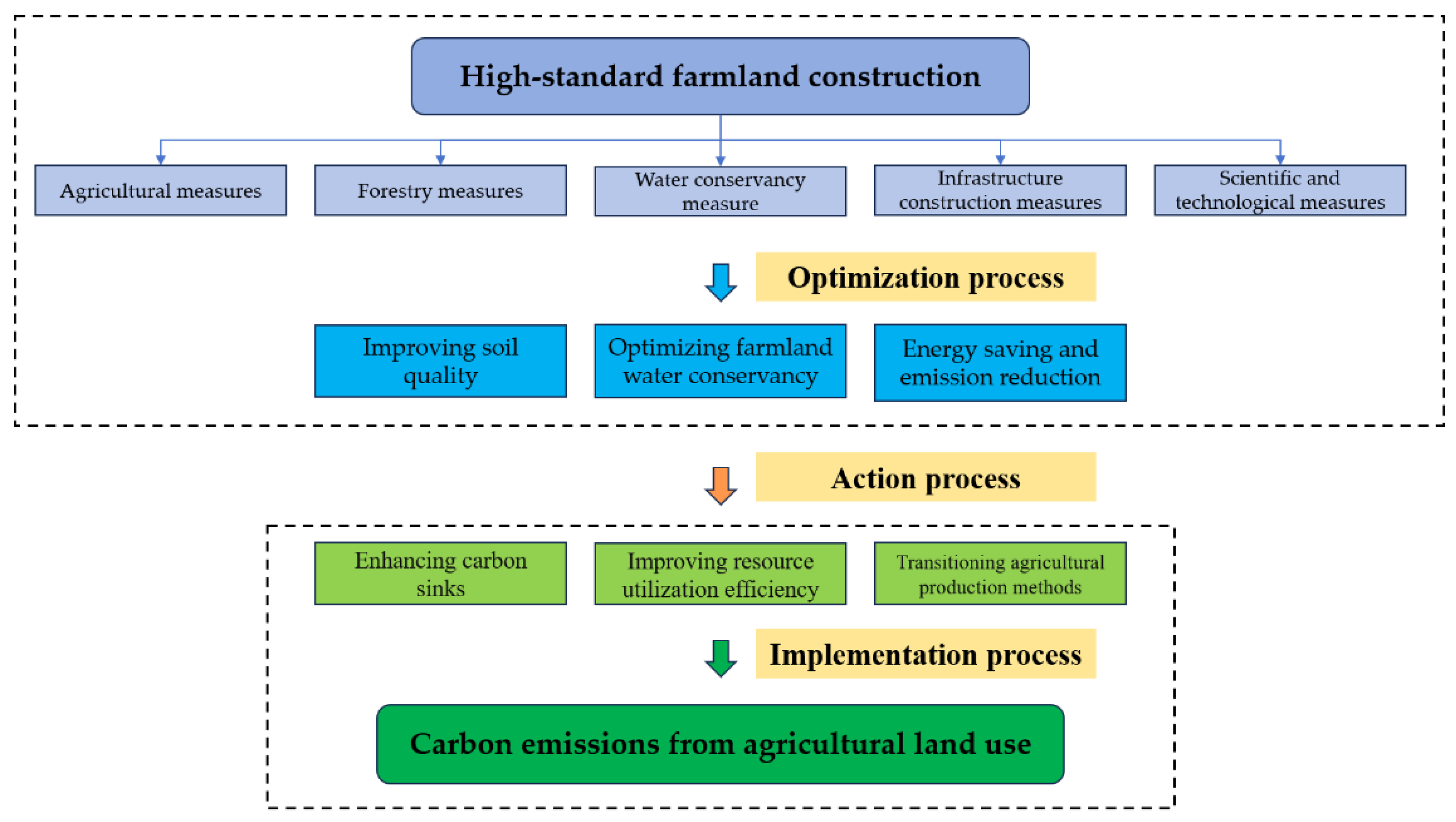
2.2. Theoretical Analysis: The Logical Relationship between HSFC and CEALU
2.2.1. Optimization Process
2.2.2. Action Process
2.2.3. Implementation Process
3. Methods and Materials
3.1. Methods
3.2. Data and Variable
3.2.1. Data Sources
3.2.2. Variable Selection
4. Results and Analysis
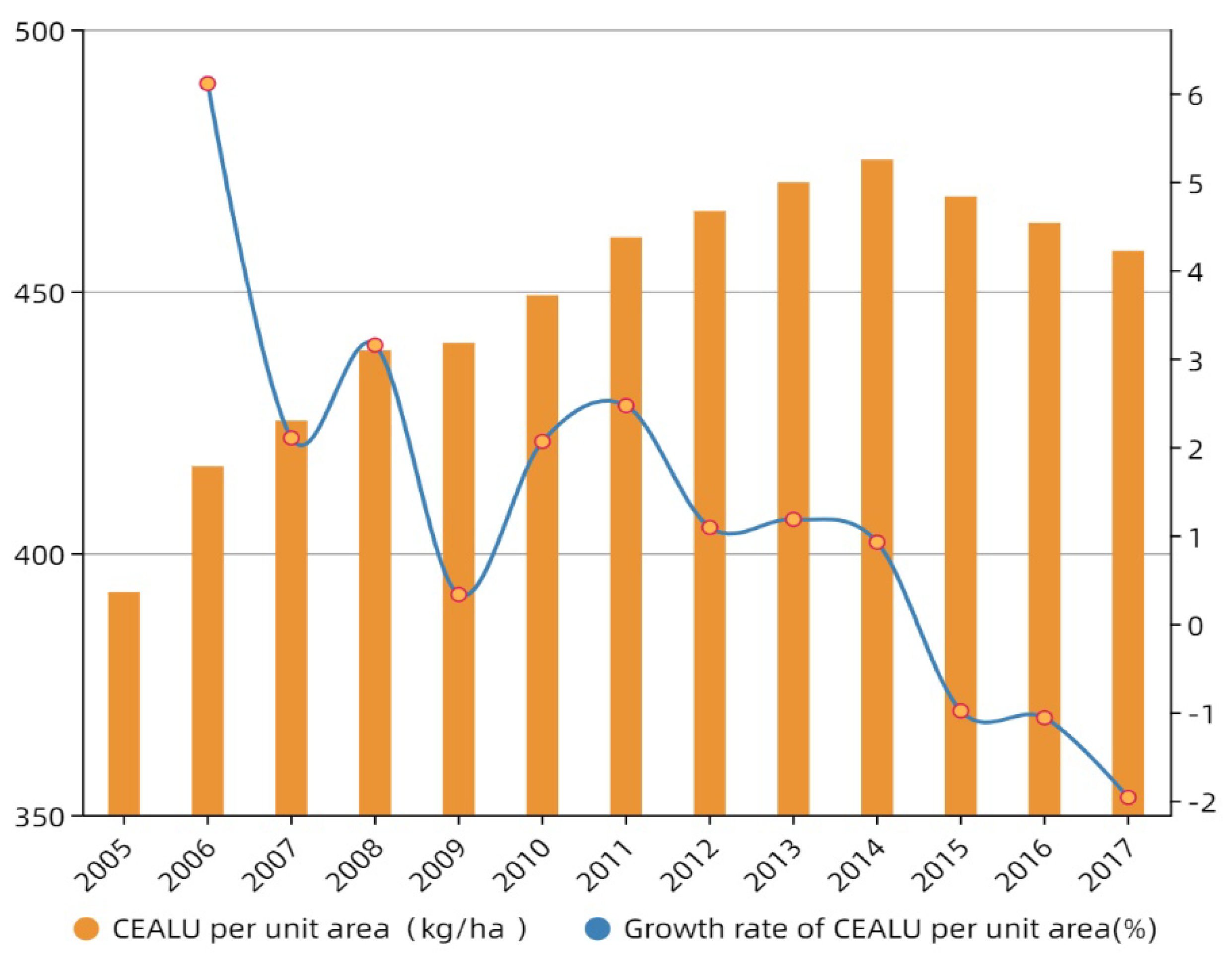
4.1. Spatiotemporal Characteristics of CEALU
4.2. Did HSFC Reduce CEALU?
4.2.1. Estimation Results of The Baseline Regression Model
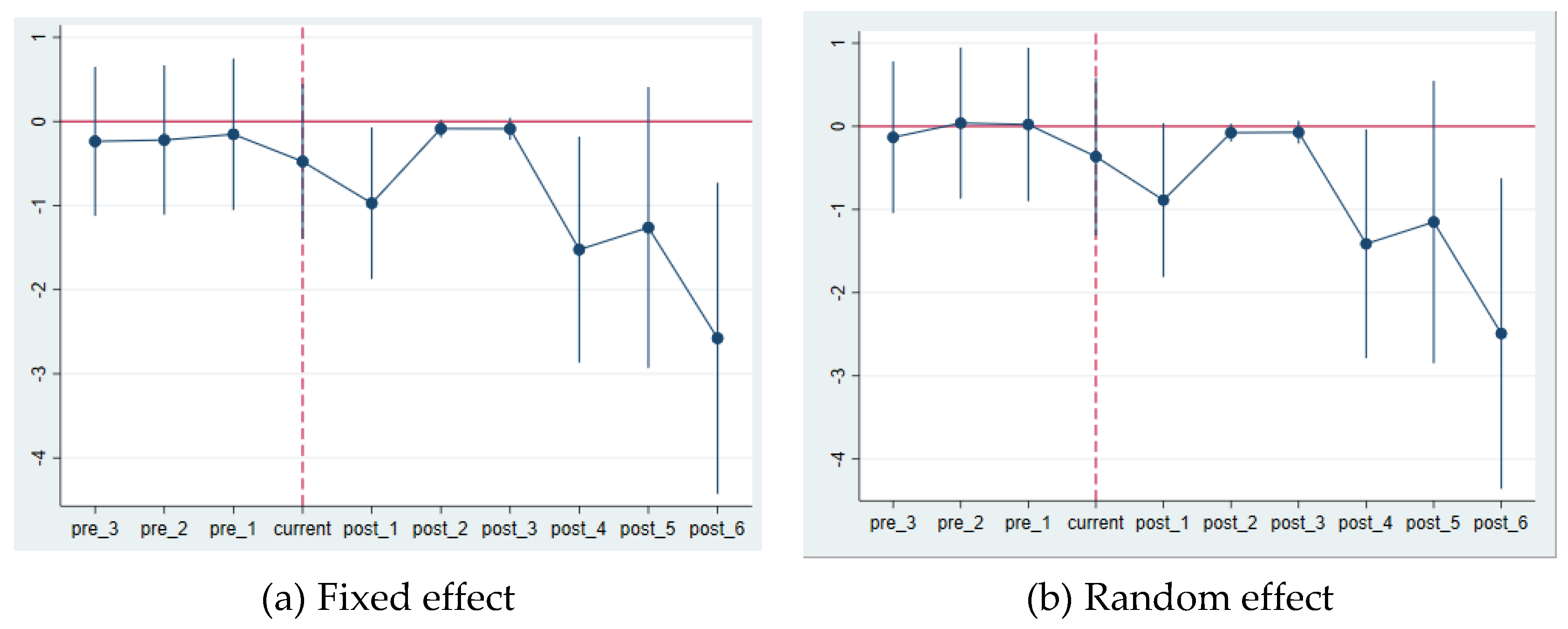
4.2.2. Parallel Trend Test and Dynamic Policy Effect
4.2.3. Robustness Test
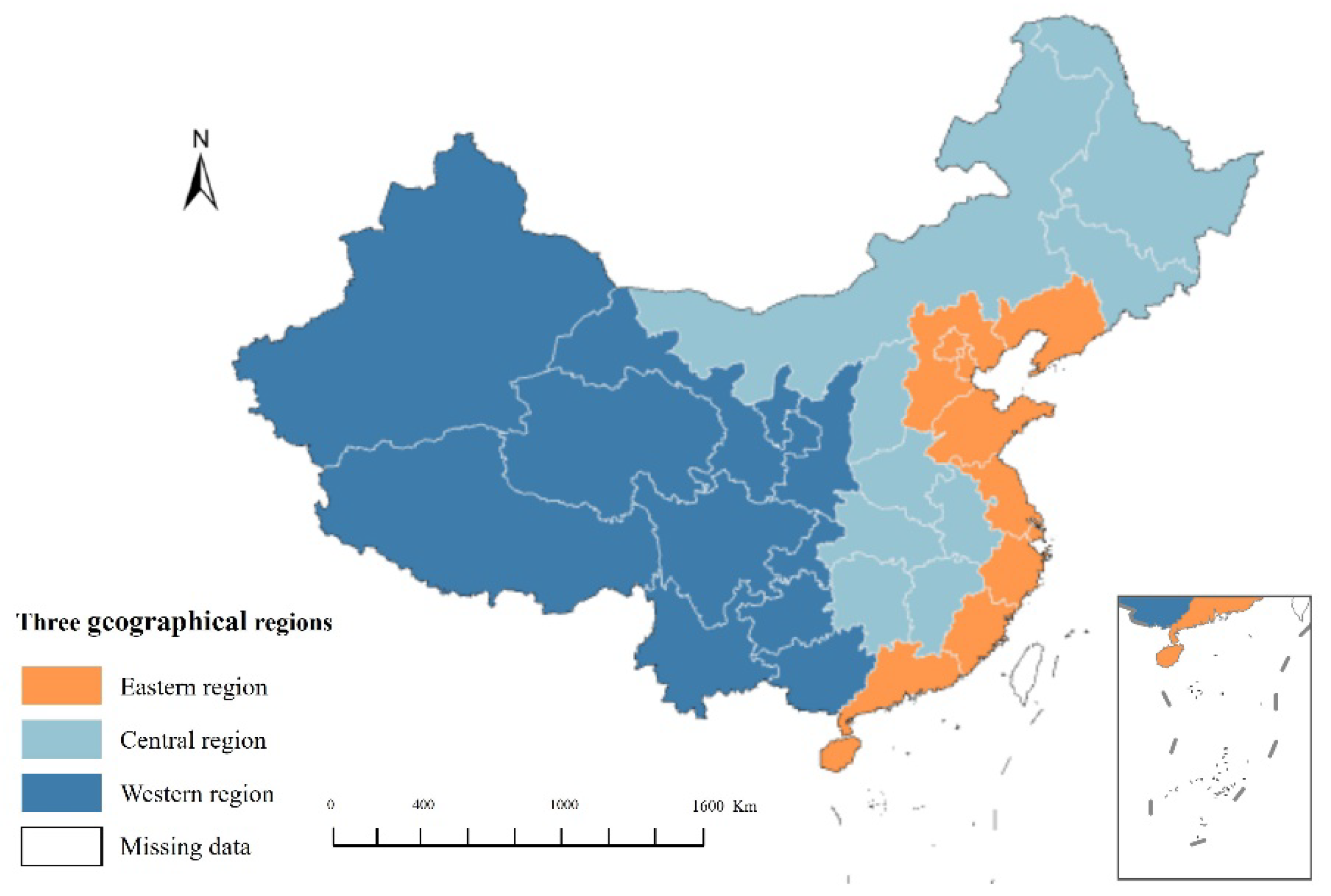
4.3. Is the Regional Heterogeneity Effect of HSFC on CEALU?
5. Discussion
6. Conclusions
Author Contributions
Funding
Data Availability Statement
Acknowledgments
Conflicts of Interest
References
- Haoyue, W.U.; Hanjiao, H.; Yu, H.; Wenkuan, C. Measurement, spatial spillover and influencing factors of agricultural carbon emissions efficiency in China. Chinese Journal of Eco-Agriculture 2021, 29, 1762–1773. [Google Scholar] [CrossRef]
- World Bank. World Development Indicators: Agricultural Methane Emissions. Available online: http://data.worldbank.org/indicator/En.Atm.Meth.Kt.Ce (accessed on 25 January 2018).
- Dumortier, J.; Elobeid, A. Effects of a carbon tax in the United States on agricultural markets and carbon emissions from land-use change. Land Use Policy 2021, 103, 105320. [Google Scholar] [CrossRef]
- Zhou, M.; Hu, B. Decoupling of carbon emissions from agricultural land utilisation from economic growth in China. Agricultural Economics (Zemědělská ekonomika) 2020, 66, 510–518. [Google Scholar] [CrossRef]
- Aruhan; Dan, M.U.; Sudesuriguge; Asina. Analysis on land use carbon emissions and influencing factors in Duolun county,Inner Mongolia. Journal of Arid Land Resources Environment 2019, 33, 17–22.
- Huang, W.; Wu, F.; Han, W.; Li, Q.; Han, Y.; Wang, G.; Feng, L.; Li, X.; Yang, B.; Lei, Y.; et al. Carbon footprint of cotton production in China: Composition, spatiotemporal changes and driving factors. Science of The Total Environment 2022, 821, 153407. [Google Scholar] [CrossRef] [PubMed]
- Liu, M.; Yang, L. Spatial pattern of China’s agricultural carbon emission performance. Ecological Indicators 2021, 133, 108345. [Google Scholar] [CrossRef]
- Su, K.; Wei, D.-z.; Lin, W.-x. Influencing factors and spatial patterns of energy-related carbon emissions at the city-scale in Fujian province, Southeastern China. Journal of Cleaner Production 2020, 244, 118840. [Google Scholar] [CrossRef]
- Xia, Q.; Liao, M.; Xie, X.; Guo, B.; Lu, X.; Qiu, H. Agricultural carbon emissions in Zhejiang Province, China (2001–2020): changing trends, influencing factors, and has it achieved synergy with food security and economic development? Environmental Monitoring and Assessment 2023, 195, 1391. [Google Scholar] [CrossRef]
- Reeve, A.; Aisbett, E. National accounting systems as a foundation for embedded emissions accounting in trade-related climate policies. Journal of Cleaner Production 2022, 371, 133678. [Google Scholar] [CrossRef]
- Chen, Y.; Li, S.; Cheng, L. Evaluation of Cultivated Land Use Efficiency with Environmental Constraints in the Dongting Lake Eco-Economic Zone of Hunan Province, China. Land 2020, 9, 440. [Google Scholar] [CrossRef]
- Yang, H.; Wang, X.; Bin, P. Agriculture carbon-emission reduction and changing factors behind agricultural eco-efficiency growth in China. Journal of Cleaner Production 2022, 334, 130193. [Google Scholar] [CrossRef]
- Panchasara, H.; Samrat, N.H.; Islam, N. Greenhouse Gas Emissions Trends and Mitigation Measures in Australian Agriculture Sector—A Review. Agriculture 2021, 11, 85. [Google Scholar] [CrossRef]
- Qichen, Z.; Dun, Y.; Jianping, W. Spatial and temporal evolution, influencing factors and trend prediction of carbon emissions from agricultural land use in JiuJiang city. Research of Soil and Water Conservation 2023, 30, 441–451. [Google Scholar] [CrossRef]
- Dumortier, J.; Elobeid, A. Effects of a carbon tax in the United States on agricultural markets and carbon emissions from land-use change. Land use policy 2021, 103, 105320. [Google Scholar] [CrossRef]
- Bai, Y.; Wang, Y.; Xuan, X.; Weng, C.; Huang, X.; Deng, X. Tele-connections, driving forces and scenario simulation of agricultural land, water use and carbon emissions in China's trade. Resources, Conservation and Recycling 2024, 203, 107433. [Google Scholar] [CrossRef]
- XinWei, L.; Jingyu, L.; Cuili, Z. On building 4 hundred million mu of high-standard basic farmland in the twelfth five-year plan. China Population,Resources and Environment 2012, 22, 1–5. [Google Scholar]
- Xue-ying, M.A.; Jing-an, S.H.O.; Fei, C.A. Comprehensive Performance Evaluation of High Standard Farmland Construction in Mountainous Counties—A Case Study in Dianjiang, Chongqing. Journal of Natural Resources 2018, 33, 2183–2199. [Google Scholar] [CrossRef]
- Liu, Y.; Liao, W.; Zhang, X.; Qiu, H. Impact of high standard farmland construction policy on chemical fertilizer reduction: a case study of China. Frontiers in Environmental Science 2023, 11. [Google Scholar] [CrossRef]
- Ye, F.; Wang, L.; Razzaq, A.; Tong, T.; Zhang, Q.; Abbas, A. Policy Impacts of High-Standard Farmland Construction on Agricultural Sustainability: Total Factor Productivity-Based Analysis. Land 2023, 12, 283. [Google Scholar] [CrossRef]
- Li, X.; He, Y.; Fu, Y.; Wang, Y. Analysis of the carbon effect of high-standard basic farmland based on the whole life cycle. Sci Rep. 2024, 14, 3361. [Google Scholar] [CrossRef]
- Ministry of Agriculture and Rural Affairs of the People's Republic of China.Well-facilitated Farmland Construction—General rules. Available online: http://www.moa.gov.cn/ztzl/gdzlbhyjs/mtbd_28775/mtbd/202204/t20220418_6396631.htm (accessed on 9 March 2018).
- Wang, X.; Shi, W.; Sun, X.; Wang, M. Comprehensive benefits evaluation and its spatial simulation for well-facilitated farmland projects in the Huang-Huai-Hai Region of China. Land Degradation & Development 2020, 31, 1837–1850. [Google Scholar] [CrossRef]
- Hu, Y.C.; Lu, X.L.; Zhao, G.L. Construction scale and spatial distribution of well-facilitated primary farmland of daxian county in sichuan province. China Land Sciences 2014, 28, 30–38. [Google Scholar] [CrossRef]
- Shan, W.; Jin, X.; Yang, X.; Gu, Z.; Han, B.; Li, H.; Zhou, Y. A framework for assessing carbon effect of land consolidation with life cycle assessment: A case study in China. Journal of Environmental Management 2020, 266, 110557. [Google Scholar] [CrossRef] [PubMed]
- Yang, Y.; Cao, T. Measurement of carbon effect in land consolidation projects and evaluation of low-carbon promotion paths: a case study of Wudi County, Shandong Province, China. Environ Sci Pollut Res Int 2023, 30, 113068–113087. [Google Scholar] [CrossRef] [PubMed]
- Xin, G.; Yang, C.; Yang, Q.; Li, C.; Wei, C. Post-evaluation of well-facilitied capital farmland construction based on entropy weight method and improved TOPSIS model. Transactions of the Chinese Society of Agricultural Engineering 2017, 33, 238–249. [Google Scholar]
- Zhihui, L.; Lu, Z.; Junbiao, Z. Land consolidation and fertilizer reduction: Quasi-natural experimental evidence from china’s well-facilitated capital farmland construction. Chinese Rural Economy 2021, 123–144. [Google Scholar]
- Zhang, L.; Liang, Z.H.; Pu, Y.X. Effect and improvement of soil testing and formulated fertilization technology in the Yangtze River Economic Belt. Journal of Huazhong Agricultural University 2021, 40, 30–42. [Google Scholar] [CrossRef]
- Liu, C.; Wu, Y.; Wang, C. Zoning method for well-facilitated farmland construction based on improvement of ecological services. Transactions of the Chinese Society of Agricultural Engineering 2018, 34, 264–272. [Google Scholar] [CrossRef]
- Tian'En, Z.; Zijie, L.I.; Kun, F. Effects of high-standard farmland construction on farmland quality and contribution of irrigation and drainage index. Journal of Agricultural Resources and Environment 2022, 39, 978–989. [Google Scholar] [CrossRef]
- Jibin, Z.; JingAn, S.; Deti, X. Dynamic changes of soil organic carbon for basic farmland and non-basic farmland of Dianjiang county in recent 30 years. Transactions of the Chinese Society of Agricultural Engineering 2016, 32, 254–262. [Google Scholar]
- Soulé, E.; Charbonnier, R.; Schlosser, L.; Michonneau, P.; Michel, N.; Bockstaller, C. A new method to assess sustainability of agricultural systems by integrating ecosystem services and environmental impacts. Journal of Cleaner Production 2023, 415, 137784. [Google Scholar] [CrossRef]
- Jiansheng, L.; Wenju, Y.; Xiaomin, Z.; Xinwen, L. Theory and Application of Well-facilitied Capital Farmland Construction: An Analysis Based on the Gap Degree and Investment Intensity. China Population Resources and Environment 2014, 24, 47–53. [Google Scholar]
- Song, W.; Wu, K.; Zhao, H.; Zhao, R.; Li, T. Arrangement of High-standard Basic Farmland Construction Based on Village-region Cultivated Land Quality Uniformity. Chinese Geographical Science 2019, 29, 325–340. [Google Scholar] [CrossRef]
- Středová, H.; Středa, T.; Rožnovský, J. Long-term comparison of climatological variables used for agricultural land appraisement. Contributions to Geophysics and Geodesy 2013, 43, 179–195. [Google Scholar] [CrossRef]
- Li, J.; Wang, W.; Li, M.; Li, Q.; Liu, Z.; Chen, W.; Wang, Y. Impact of Land Management Scale on the Carbon Emissions of the Planting Industry in China. Land 2022, 2022, 816. [Google Scholar] [CrossRef]
- Carvalheiro, L.G.; Veldtman, R.; Shenkute, A.G.; Tesfay, G.B.; Pirk, C.W.W.; Donaldson, J.S.; Nicolson, S.W. Natural and within-farmland biodiversity enhances crop productivity. Ecology Letters 2011, 14, 251–259. [Google Scholar] [CrossRef] [PubMed]
- Wu, Q.; Xiong, K.; Li, R.; Xiao, J. Farmland hydrology cycle and agronomic measures in agroforestry for the efficient utilization of water resources under karst desertification environments. Forests 2023, 14, 453. [Google Scholar] [CrossRef]
- Xiao, M.; Li, Y.; Zheng, S. Effect of Rural Sewage Irrigation Regime on Water-Nitrogen Utilization and Crop Growth of Paddy Rice in Southern China. Phyton-International Journal of Experimental Botany 2023, 92. [Google Scholar] [CrossRef]
- Ke, Z.; Liu, X.; Ma, L.; Dong, Q.g.; Jiao, F.; Wang, Z. Excavated farmland treated with plastic mulching as a strategy for groundwater conservation and the control of soil salinization. Land Degradation & Development 2022, 33, 3036–3048. [Google Scholar] [CrossRef]
- Yang, N.; Sun, X.; Qi, Q. Impact of factor quality improvement on agricultural carbon emissions: Evidence from China’s high-standard farmland. Frontiers in Environmental Science 2022, 10. [Google Scholar] [CrossRef]
- Cao, X.F.; Sun, B.; Chen, H.B.; et al. Approaches and Research Progresses of Marginal Land Productivity Expansion and Ecological Benefit Improvement in China. Bulletin of Chinese Academy of Sciences 2021, 36, 336–348. [Google Scholar] [CrossRef]
- Ustaoglu, E.; Collier, M.J. Farmland abandonment in Europe: an overview of drivers, consequences, and assessment of the sustainability implications. Environmental Reviews 2018, 26, 396–416. [Google Scholar] [CrossRef]
- The State Council. Trial Measures For The Administration Of Recovery Of National Land Development And Construction Funds. Available online: https://xueshu.baidu.com/usercenter/paper/show?paperid=a5583c0a75fcd7235c0f4719edbd893b&tn=SE_baiduxueshu_c1gjeupa&ie=utf-8&site=baike (accessed on 27 August 2018).
- Central Government of the People's Republic of China. China's No. 1 Central Document: Opinions on several policies to further strengthen rural work and improve the overall agricultural production capacity. Available online: https://www.gov.cn/test/2006-02/22/content_207406.htm (accessed on 30 January 2015).
- National Development and Reform Commission. The National High-Standard Farmland Construction Plan (2021-2030). Available online: https://www.ndrc.gov.cn/fggz/fzzlgh/gjjzxgh/202111/t20211102_1302810.html (accessed on 2 November 2015).
- Haitao, L. Ocus on the green development of Agriculture and Help achieve the Goal of "Double carbon" -- A review of China's Agricultural Carbon Emission Reduction Path Study. Issues in Agricultural Economy 2022, 144. [Google Scholar] [CrossRef]
- Yu, S.; Weiping, L.; Zhen, X. Model evaluation of the impact of high-standard farmland construction policy on planting structure. Transactions of the Chinese Society of Agricultural Engineering 2023, 39, 227–235. [Google Scholar] [CrossRef]
- Zhao, R.; Wu, K. Soil Health Evaluation of Farmland Based on Functional Soil Management—A Case Study of Yixing City, Jiangsu Province, China. Agriculture 2021, 11, 583. [Google Scholar] [CrossRef]
- Qiao, L.; Wang, X.; Smith, P.; et al. Soil quality both increases crop production and improves resilience to climate change. Nature Climate Change 2022, 12, 574–580. [Google Scholar] [CrossRef]
- Tianjiao, F.; Dong, W.; Ruoshui, W.; Yixin, W.; Zhiming, X.; Fengmin, L.; Yuan, M.; Xing, L.; Huijie, X.; Caballero-Calvo, A.; et al. Spatial-temporal heterogeneity of environmental factors and ecosystem functions in farmland shelterbelt systems in desert oasis ecotones. Agricultural Water Management 2022, 271, 107790. [Google Scholar] [CrossRef]
- Sang, Z.; Zhang, G.; Wang, H.; Zhang, W.; Chen, Y.; Han, M.; Yang, K. Effective Solutions to Ecological and Water Environment Problems in the Sanjiang Plain: Utilization of Farmland Drainage Resources. Sustainability 2023, 15. [Google Scholar] [CrossRef]
- Penghui, J.; Dengshuai, C.; Manchun, L. Farmland landscape fragmentation evolution and its driving mechanism from rural to urban: A case study of Changzhou City. Journal of Rural Studies 2021, 82, 1–18. [Google Scholar] [CrossRef]
- Sardaro, R.; Bozzo, F.; Fucilli, V. High-voltage overhead transmission lines and farmland value: Evidences from the real estate market in Apulia, southern Italy. Energy Policy 2018, 119, 449–457. [Google Scholar] [CrossRef]
- Song, W.; Wu, K.; Zhao, H.; et al. Arrangement of High-standard Basic Farmland Construction Based on Village-region Cultivated Land Quality Uniformity. Chinese Geographical Science 2019, 29, 325–340. [Google Scholar] [CrossRef]
- Shen, Z.; Wang, S.; Boussemart, J.-P.; Hao, Y. Digital transition and green growth in Chinese agriculture. Technological Forecasting and Social Change 2022, 181, 121742. [Google Scholar] [CrossRef]
- Coomes, O.T.; Barham, B.L.; MacDonald, G.K.; et al. Leveraging total factor productivity growth for sustainable and resilient farming. Nature Sustainability 2019, 2, 22–28. [Google Scholar] [CrossRef]
- Frank, S.; Havlík, P.; Stehfest, E.; van Meijl, H.; Witzke, P.; Pérez-Domínguez, I.; van Dijk, M.; Doelman, J.C.; Fellmann, T.; Koopman, J.F.L.; et al. Agricultural non-CO2 emission reduction potential in the context of the 1.5 °C target. Nature Climate Change 2019, 9, 66–72. [Google Scholar] [CrossRef]
- Shang, Q.; Ling, N.; Feng, X.; Yang, X.; Wu, P.; Zou, J.; Shen, Q.; Guo, S. Soil fertility and its significance to crop productivity and sustainability in typical agroecosystem: a summary of long-term fertilizer experiments in China. Plant and Soil 2014, 381, 13–23. [Google Scholar] [CrossRef]
- Chen, B.; Han, M.Y.; Peng, K.; Zhou, S.L.; Shao, L.; Wu, X.F.; Wei, W.D.; Liu, S.Y.; Li, Z.; Li, J.S.; et al. Global land-water nexus: Agricultural land and freshwater use embodied in worldwide supply chains. Science of The Total Environment 2018, 613-614, 931–943. [Google Scholar] [CrossRef] [PubMed]
- Zhao, R.; Liu, Y.; Tian, M.; Ding, M.; Cao, L.; Zhang, Z.; Chuai, X.; Xiao, L.; Yao, L. Impacts of water and land resources exploitation on agricultural carbon emissions: The water-land-energy-carbon nexus. Land Use Policy 2018, 72, 480–492. [Google Scholar] [CrossRef]
- Yang, Y.; Jin, Z.; Mueller, N.D.; Driscoll, A.W.; Hernandez, R.R.; Grodsky, S.M.; Sloat, L.L.; Chester, M.V.; Zhu, Y.-G.; Lobell, D.B. Sustainable irrigation and climate feedbacks. Nature Food 2023, 4, 654–663. [Google Scholar] [CrossRef] [PubMed]
- Zomer, R.J.; Bossio, D.A.; Sommer, R.; Verchot, L.V. Global sequestration potential of increased organic carbon in cropland soils. Scientific Reports 2017, 7, 15554. [Google Scholar] [CrossRef]
- Auerswald, K.; Fischer, F.K.; Kistler, M.; Treisch, M.; Maier, H.; Brandhuber, R. Behavior of farmers in regard to erosion by water as reflected by their farming practices. Science of The Total Environment 2018, 613-614, 1–9. [Google Scholar] [CrossRef]
- Shah, K.K.; Modi, B.; Pandey, H.P.; Subedi, A.; Aryal, G.; Pandey, M.; Shrestha, J.; Fahad, S. Diversified Crop Rotation: An Approach for Sustainable Agriculture Production. Advances in Agriculture 2021, 1–9. [Google Scholar] [CrossRef]
- Barbieri, P.; Pellerin, S.; Nesme, T. Comparing crop rotations between organic and conventional farming. Scientific Reports 2017, 7, 13761. [Google Scholar] [CrossRef] [PubMed]
- Vejan, P.; Khadiran, T.; Abdullah, R.; Ahmad, N. Controlled release fertilizer: A review on developments, applications and potential in agriculture. Journal of Controlled Release 2021, 339, 321–334. [Google Scholar] [CrossRef] [PubMed]
- Han, H.; Zhong, Z.; Guo, Y.; Xi, F.; Liu, S. Coupling and decoupling effects of agricultural carbon emissions in China and their driving factors. Environmental Science and Pollution Research 2018, 25, 25280–25293. [Google Scholar] [CrossRef] [PubMed]
- Coomes, O.T.; Barham, B.L.; MacDonald, G.K.; Ramankutty, N.; Chavas, J.-P. Leveraging total factor productivity growth for sustainable and resilient farming. Nature Sustainability 2019, 2, 22–28. [Google Scholar] [CrossRef]
- Weersink, A.; Fraser, E.; Pannell, D.; Duncan, E.; Rotz, S. Opportunities and Challenges for Big Data in Agricultural and Environmental Analysis. Annual Review of Resource Economics 2018, 10, 19–37. [Google Scholar] [CrossRef]
- Bi, X.; Wen, B.; Zou, W. The Role of Internet Development in China’s Grain Production: Specific Path and Dialectical Perspective. Agriculture 2022, 12, 377. [Google Scholar] [CrossRef]
- Patrício, D.I.; Rieder, R. Computer vision and artificial intelligence in precision agriculture for grain crops: A systematic review. Computers and Electronics in Agriculture 2018, 153, 69–81. [Google Scholar] [CrossRef]
- Ministry of Finance of The People's Republic of China. Doing a Good Job in the Implementation of the National High-standard Farmland Construction Plan for Comprehensive Agricultural Development and Vigorously Promoting High-standard Farmland Construction. Available online: http://nfb.mof.gov.cn/zhengwuxinxi/gongzuotongzhi/201304/t20130410_816024.html (accessed on 16 March 2013).
- Kuang, B.; Lu, X.H.; Zhou, M. Dynamic Evolution of Urban Land Economic Density Distributionin China. China Land Science 2016, 30, 47–54. [Google Scholar] [CrossRef]
- Nie, Y.; Li, Q.; Wang, E.; Zhang, T. Study of the nonlinear relations between economic growth and carbon dioxide emissions in the Eastern, Central and Western regions of China. Journal of Cleaner Production 2019, 219, 713–722. [Google Scholar] [CrossRef]
- Delgado, M.S.; Florax, R.J.G.M. Difference-in-differences techniques for spatial data: Local autocorrelation and spatial interaction. Economics Letters 2015, 137, 123–126. [Google Scholar] [CrossRef]
- Zheng, W.; Shen, G.Q.; Wang, H.; Hong, J.; Li, Z. Decision support for sustainable urban renewal: A multi-scale model. Land Use Policy 2017, 69, 361–371. [Google Scholar] [CrossRef]
- Stuart, E.A.; Huskamp, H.A.; Duckworth, K.; Simmons, J.; Song, Z.; Chernew, M.; Barry, C.L. Using propensity scores in difference-in-differences models to estimate the effects of a policy change. Health services & outcomes research methodology 2014, 14, 166–182. [Google Scholar] [CrossRef]
- Guixin, X.; Chaoxian, Y.; Qingyuan, Y.; et al. Post-evaluation of well-facilitied capital farmland construction based on entropy weight method and improved TOPSIS model. Transactions of the Chinese Society of Agricultural Engineering 2017, 33, 238–249. [Google Scholar] [CrossRef]
- Zhang, T.; Li, Z.J.; Fei, K.; et al. Effects of high-standard farmland construction on farmland quality and contribution of irrigation and drainage index. Journal of Agricultural Resources and Environment 2022, 39, 978–989. [Google Scholar] [CrossRef]
- Kuang, B.; Lu, X.H.; Han, J.; et al. Regional differences and dynamic evolution of cultivated land use efficiency in major grain producing areas in low carbon perspective. Transactions of the Chinese Society of Agricultural Engineering 2018, 34, 1–8. [Google Scholar] [CrossRef]
- Johnson, J.M.F.; Franzluebbers, A.J.; Weyers, S.L.; Reicosky, D.C. Agricultural opportunities to mitigate greenhouse gas emissions. Environmental Pollution 2007, 150, 107–124. [Google Scholar] [CrossRef] [PubMed]
- West, T.O.; Marland, G. A synthesis of carbon sequestration, carbon emissions, and net carbon flux in agriculture: comparing tillage practices in the United States. Agriculture, Ecosystems & Environment 2002, 91, 217–232. [Google Scholar] [CrossRef]
- Lu, X.; Kuang, B.; Li, J.; Han, J.; Zhang, Z. Dynamic Evolution of Regional Discrepancies in Carbon Emissions from Agricultural Land Utilization: Evidence from Chinese Provincial Data. Sustainability 2018, 10. [Google Scholar] [CrossRef]
- Tian, Y.; Zhang, J.-b.; He, Y.-y. Research on Spatial-Temporal Characteristics and Driving Factor of Agricultural Carbon Emissions in China. Journal of Integrative Agriculture 2014, 13, 1393–1403. [Google Scholar] [CrossRef]
- Han, H.; Zhong, Z.; Guo, Y.; Xi, F.; Liu, S. Coupling and decoupling effects of agricultural carbon emissions in China and their driving factors. Environmental Science and Pollution Research 2018, 25, 25280–25293. [Google Scholar] [CrossRef] [PubMed]
- Dubey, A.; Lal, R. Carbon Footprint and Sustainability of Agricultural Production Systems in Punjab, India, and Ohio, USA. Journal of Crop Improvement 2009, 23, 332–350. [Google Scholar] [CrossRef]
- HE, Y.Q.; CHEN, R.; WU, H.Y.; XU, J.; SONG, Y. Spatial dynamics of agricultural carbon emissions in China and the related driving factors. Chinese Journal of Eco-Agriculture 2018, 26, 1269–1282. [Google Scholar] [CrossRef]
- Chen, Y.B.; Wang, S. Evaluation of Agricultural Carbon Emission Reduction Effect of Agricultural Comprehensive Development Investment :Event Analysis Based on High-standard Farmland Construction. Journal of Agrotechnical economy 2023, 67–80. [Google Scholar] [CrossRef]
- Tao, L.; Jixia, L.I.; Jingjuan, H. Spatial-temporal pattern and influencing factors of high-quality agricultural development in China. Journal of Arid Land Resources and Environment 2020, 34, 1–8. [Google Scholar] [CrossRef]
- Gong, Y.L.; Zhang, Y.L. Influence of well-facilitated capital farmland construction policy on grain productivity. Journal of Huazhong Agricultural University (Social Sciences Edition) 2023, 175–190. [Google Scholar] [CrossRef]
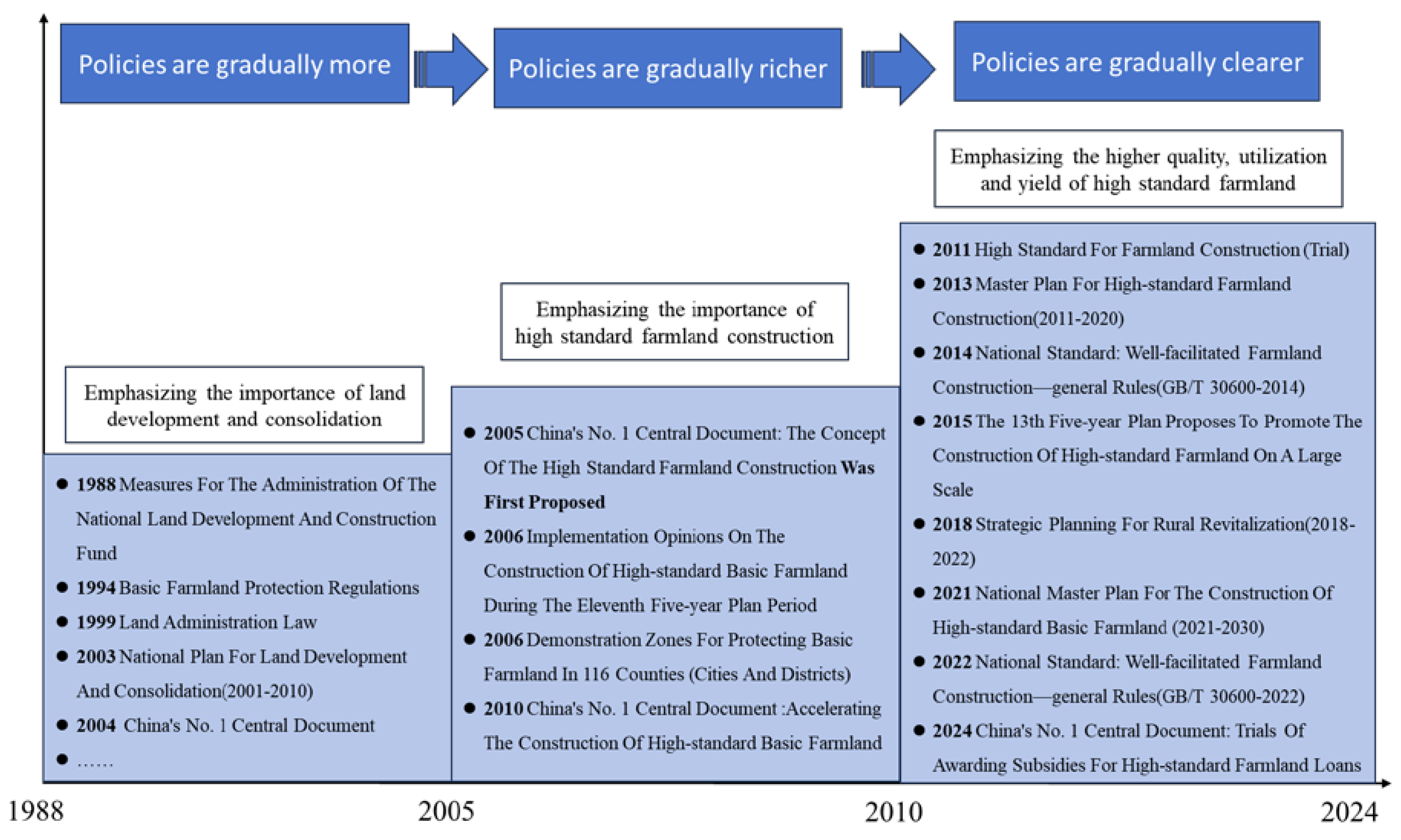
| Standards | Contents | Zoning | Objectives | Safeguard Measures |
|---|---|---|---|---|
| GB/T 33130-2016 | Farmland Consolidation | Northeast Region | 1.075 billion Mu (2025) | Government Overall Planning |
| GB/T33469-2016 | Soil Improvement | Huang-Huai-Hai Area | 1.2 billion Mu (2030) | Planning Guidance |
| GB/T 21010-2017 | Irrigation And Drainage | The Middle and Lower Reaches of The Yangtze River | Fund Guarantee | |
| GB 50288-2018 | Field Road | Southeast Region |
Scientific and Technological Support | |
| GB 5084-2021 | Agricultural Field Protection Ecological and Environmental Protection | Southwest Region | Supervision and Assessment | |
| GB/ T 30600-2022 | Farmland Power Transmission and Distribution | Northwest Region | ||
| ...... | Science and Technology Service | Qinghai-Tibet Region | ||
| Management, Protection and Utilization |
| Measures | Content | Purpose |
|---|---|---|
| Agricultural measures | Farmland Consolidation | Optimize the spatial distribution of high-standard farmland |
| Soil Improvement | Improve the quality of cultivated land | |
| Forestry measures | Protection forest of agriculture and forestry system | Improve soil and water conservation and flood control |
| Water conservancy measure | Irrigation project | Improve the guarantee rate of agricultural irrigation |
| Drainage works | Improve the ability to withstand storms | |
| Infrastructure construction measures | Field road construction | Improve the direct access road network to farmland |
| Farmland electricity transmission and distribution | Improve the quality and safety of electricity use | |
| Scientific and technological measures | Location monitoring of cultivated land quality | Tracking and monitoring the change of farmland quality |
| Digital farmland construction | Improve the level of precision and wisdom |
| Carbon Sources | Emission Coefficient | Unit | References |
|---|---|---|---|
| Chemical fertilizer | 0.8956 | Kg C /kg | West and Marland [84] |
| Pesticide | 4.9341 | Kg C /kg | Lu et al [85] |
| Thin film | 5.180 | Kg C /kg | Tian et al [86] |
| Total power of agricultural machinery | 0.18 | kg C/kW | Kuang et al [82] |
| Tillage over | 312.6 | kg C/ha | Han et al [87] |
| Irrigation | 25 | kg C/ha | Dubey et al [88] |
| Variable names, symbols, and meanings | Average value | Standard deviation | Min. | Max. |
|---|---|---|---|---|
| CEALU per unit area (C) , kg/ha | 482.22 | 182.04 | 170.16 | 1154.36 |
| Proportion of land consolidation area (Hrate) , % | 0.05 | 0.09 | 0.00 | 0.97 |
| Urbanization leve l(Urban) , Urban population as a percentage of total population , % | 0.52 | 0.14 | 0.20 | 0.89 |
| Soil quality (Soil) , Soil erosion control area , kha | 3490.75 | 2847.04 | 0.00 | 13600 |
| Field irrigation condition (Irri) , Effective irrigation area , kha | 1991.36 | 1537.66 | 115.50 | 6031.00 |
| Per unit area yield of grain (Fyield) , Grain output per unit area , kg/ha | 5149.15 | 996.90 | 3045.73 | 7885.95 |
| Investment level (Ginves) , Investment in fixed assets of the whole society , 100 million yuan | 374.11 | 418.17 | 3045.73 | 2675.94 |
| The proportion of food crops (Frate) , Proportion of grain sown area to total sown area , % | 65.36 | 12.46 | 3045.73 | 2675.94 |
| Labor input (Labor) , Headcount in primary industry , 10 thousand people | 938.83 | 694.87 | 37.09 | 3139.00 |
| Economic development level (GDP) , PGDP , yuan | 28300 | 17800 | 5200.80 | 107000 |
| industrial structure (Grate) , Proportion of agricultural output value to GDP , % | 10.99 | 5.63 | 0.36 | 32.73 |
| Area | 2005 | 2008 | 2011 | 2014 | 2017 | Mean | Area | 2005 | 2008 | 2011 | 2014 | 2017 | Mean |
|---|---|---|---|---|---|---|---|---|---|---|---|---|---|
| Beijing | 692.91 | 689.35 | 721.74 | 931.61 | 1154.36 | 819.42 | Hubei | 476.93 | 549.49 | 536.44 | 518.28 | 481.99 | 520.93 |
| Tianjin | 613.26 | 717.79 | 669.49 | 627.22 | 544.22 | 660.25 | Hunan | 356.47 | 399.14 | 387.07 | 385.34 | 399.75 | 390.27 |
| Hebei | 438.18 | 456.72 | 471.19 | 493.86 | 487.03 | 471.80 | Guangdong | 518.95 | 629.81 | 660.01 | 652.18 | 749.90 | 648.97 |
| Shanxi | 313.68 | 343.16 | 377.01 | 403.82 | 406.91 | 374.96 | Guangxi | 346.64 | 441.30 | 459.70 | 500.09 | 508.27 | 459.05 |
| Neimenggu | 228.03 | 266.28 | 298.74 | 369.06 | 319.80 | 300.91 | Hainan | 619.51 | 836.73 | 916.64 | 925.86 | 1097.88 | 889.25 |
| Liaoning | 481.58 | 547.38 | 572.56 | 592.53 | 548.95 | 555.46 | Chongqing | 282.97 | 336.16 | 348.73 | 344.49 | 361.51 | 338.94 |
| Ji Lin. | 333.86 | 397.49 | 447.04 | 478.55 | 449.14 | 427.71 | Sichuan | 297.99 | 329.08 | 343.88 | 342.65 | 337.41 | 334.26 |
| Heilongjiang | 195.77 | 197.50 | 243.45 | 270.30 | 222.17 | 228.78 | Guizhou | 193.13 | 237.16 | 233.98 | 230.81 | 218.67 | 226.15 |
| Shanghai | 753.55 | 735.05 | 626.80 | 616.84 | 646.23 | 661.50 | Yunnan | 303.82 | 357.00 | 385.79 | 411.49 | 450.27 | 383.14 |
| Jiangsu | 531.30 | 543.64 | 538.28 | 526.27 | 504.84 | 532.59 | Xizang. | 214.26 | 240.32 | 251.63 | 276.11 | 285.40 | 257.25 |
| Zhejiang | 510.28 | 594.30 | 605.45 | 650.67 | 689.49 | 620.92 | Shaanxi | 366.24 | 415.65 | 517.35 | 560.34 | 595.61 | 501.90 |
| Anhui | 387.17 | 423.06 | 455.02 | 476.86 | 458.54 | 444.99 | Gansu | 330.68 | 368.44 | 467.26 | 529.08 | 520.77 | 450.96 |
| Fujian | 640.41 | 765.42 | 745.20 | 750.24 | 1068.85 | 796.57 | Qinghai | 179.90 | 187.43 | 220.85 | 252.42 | 249.41 | 217.37 |
| Jiangxi | 348.29 | 366.13 | 377.39 | 375.88 | 353.27 | 367.57 | Ningxia | 293.47 | 320.92 | 358.32 | 371.31 | 418.07 | 355.78 |
| Shandong | 637.42 | 646.54 | 633.58 | 609.28 | 567.59 | 627.25 | Xinjiang | 464.76 | 536.15 | 562.74 | 684.53 | 651.85 | 571.09 |
| Henan | 423.73 | 483.46 | 536.28 | 556.52 | 538.64 | 513.04 | Tatal | 392.58 | 433.03 | 456.09 | 473.32 | 457.72 | 447.45 |
| Variables | Fixed effect-based | Random effect-based | Standard error based on POLS |
|---|---|---|---|
| -0.1080** (0.0499) |
-0.1080** (0.0520) |
-0.1080** (0.0520) |
|
| -0.4620 (0.4899) |
-0.4620 (0.5104) |
-0.4620 (0.5104) |
|
| 0.3540** (0.1346) |
0.3540** (0.1402) |
0.3540** (0.1402) |
|
| -0.5375** (0.2098) |
-0.5375** (0.2186) |
-0.5375** (0.2186) |
|
| 0.2671** (0.1142) |
0.2671** (0.1190) |
0.2671** (0.1190) |
|
| -6.27E-12 (2.20 E-11) |
-6.27 E-12 (2.30 E-11) |
-6.27 E-12 (2.30 E-11) |
|
| -0.1373 (0.0937) |
0.0101 (0.0204) |
0.0101 (0.0204) |
|
| 0.0195 (0.0267) |
-0.1373 (0.0976) |
-0.1373 (0.0976) |
|
| 0.0195 (0.0267) |
0.0195 (0.0278) |
0.0195 (0.0278) |
|
| 0.0025 (0.0063) |
0.0025 (0.0066) |
0.0025 (0.0066) |
|
| Constant term | 4.4349** (1.8696) |
5.6299*** (1.8341) |
5.6299*** (1.8341) |
| Sample size | 390 | 390 | 390 |
| 0.6349 | — | 0.9701 |
| Variable | Parallel trend FE | Parallel trend RE | Parallel trend RE | Parallel trend FE | Parallel trend RE |
|---|---|---|---|---|---|
| -0.2367 (0.4503) |
-0.1323 (0.4654) |
-1.5235** (0.6830) |
-1.4123** (0.7018) |
||
| -0.2207 (0.4516) |
0.0391 (0.4639) |
-1.2614 (0.8493) |
-1.1504 (0.8668) |
||
| -0.1524 (0.4578) |
0.0219 (0.4711) |
-2.5768*** (0.9405) |
-2.4910*** (0.9524) |
||
| -0.4758 (0.4689) |
-0.3641 (0.4834) |
Constant term | 2.2557*** (0.6967) |
2.7613*** (0.6618) |
|
| -0.9722** (0.4578) |
-0.8870* (0.4721) |
Control variable | Controls | Controls | |
| -0.0857 (0.0535) |
-0.0766 (0.0552) |
Observed value | 390 | 390 | |
| -0.0872 (0.0673) |
-0.0716 (0.0692) |
F | 28.2418 | — | |
| 0.5567 | — |
| Variable | Take 2008 as the policy implementation point | Take 2009 as the policy implementation point | ||||
| (1) Fixed effect |
(2) Random effect |
(3) Mixed effect |
(1) Fixed effect |
(2) Random effect |
(3) Mixed effect |
|
| -0.7225 (0.5729) |
-0.5015 (0.5891) |
-0.7225 (0.6315) |
||||
| -0.5749 (0.4945) |
-0.4214 (0.5042) |
-0.5749 (0.5450) |
||||
| Constant term | 3.5272** (1.4690) |
3.9660*** (0.8695) |
4.5418*** (1.5904) |
3.4980** (1.5129) |
4.0173*** (0.8893) |
4.5250*** (1.6316) |
| Control variable | Controls | Controls | Controls | Controls | Controls | Controls |
| Sample size | 180 | 180 | 180 | 180 | 180 | 180 |
| 0.7062 | — | 0.9901 | ||||
| Variable | Eastern region | Central region | Western region |
|---|---|---|---|
| -0.0262 (0.0727) |
-0.3667** (0.1806) |
0.0364 (0.1527) |
|
| Constant term | 14.0595*** (1.8904) |
0.1450 (1.7205) |
3.0510*** (0.9514) |
| Control variable | Controls | Controls | Controls |
| Sample size | 130 | 104 | 156 |
| 0.6430 | 0.7796 | 0.8121 |
Disclaimer/Publisher’s Note: The statements, opinions and data contained in all publications are solely those of the individual author(s) and contributor(s) and not of MDPI and/or the editor(s). MDPI and/or the editor(s) disclaim responsibility for any injury to people or property resulting from any ideas, methods, instructions or products referred to in the content. |
© 2024 by the authors. Licensee MDPI, Basel, Switzerland. This article is an open access article distributed under the terms and conditions of the Creative Commons Attribution (CC BY) license (http://creativecommons.org/licenses/by/4.0/).


