1. Introduction
Modular steel buildings (MSBs) have become increasingly popular in the construction industry due to their numerous advantages, including cost-effectiveness, speed of construction period, and flexibility. Modular buildings are built upon the Lego matter construction approach, in which its components (modules) are fabricated in industrial units (off-site) in a factory-controlled environment system based on the customer’s request and then transferred and assembled at the construction site (on-site) in a desired configuration to form an entire building [
1,
2,
3,
4,
5,
6,
7]. Compared to the traditional on-site technique, the entire modular building’s on-site construction time is limited to assembly modules with suitable inter-module connections (IMCs). The suitable inter-module connections (IMCs) must ensure the overall stability and strength of the building, capable of withstanding loads and stresses from various sources (wind, seismic activity, and weight of the building itself); the connections should accommodate the modular nature of the building, allowing easy assembly and disassembly [
8,
9,
10]. Given the prefabricated nature of modules, connections should be designed with tolerances that account for light variations in fabrication. Idea connections should also allow for the reuse or recycling.
Modular steel buildings are severely impacted by choosing suitable inter-module connections, especially in multi-storey MSBs, when the primary load path for the transfer of forces between modules comprises inter-module connections [
11]. From a structural viewpoint, the inter-module connections (IMCs) are crucial since they affect the overall stability of modular steel buildings [
12,
13,
14]. As the on-site construction process is limited to connecting the modules, the inter-module connections (IMCs) are highly susceptible to variables such as skilled labour, environmental conditions, availability of suitable equipment, etc. [
15]. Since the modular building is a new kind of construction in terms of research and industrial practices, the main practical challenge is ensuring the safety and longevity of those structures by ensuring a complete connection between their modules.
Researchers and engineers have recently paid more attention to modular buildings’ inter-module connections (IMCs). Extensive stat-of-the-art literature studies on the structural performance of inter-module connections have been done in Refs. [
8,
11,
14,
16,
17,
18,
19,
20,
21,
22,
23,
24,
25,
26,
27,
28,
29,
30,
31,
32,
33,
34,
35,
36,
37,
38,
39]. While the internal area between the adjacent modules is still the most prone, various (internal) inter-module connection techniques have been proposed in the available literature that aims for easy and fast installations using bolted, shear keys, plates, grouts, etc. [
10,
29,
40,
41,
42,
43,
44,
45,
46,
47,
48,
49,
50]. Generally, the two forms of inter-module connections (IMCs) are horizontal and vertical connections, where the floor beams of the upper modules and the ceiling beams of the lower modules are connected horizontally; the vertical connection for corner support modules involves joining the upper module to the lower module at corner columns. Corfar et al. [
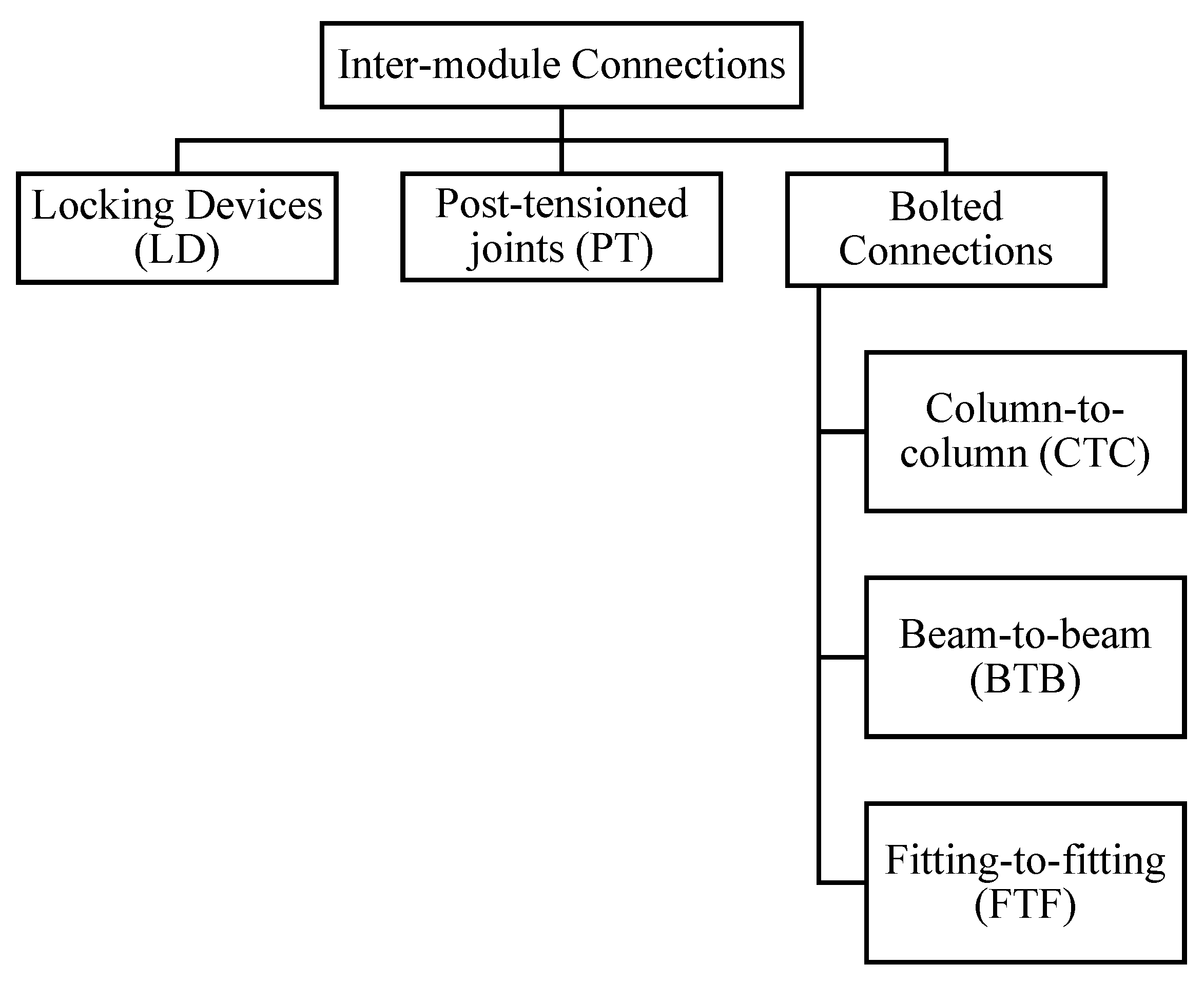
51] classified the inter-module connections (IMCs) into three main groups, as shown in
Figure 1. The most common method for connecting the top and lower modules is shear keys with gusset plates or fastened gusset plates [
52,
53]. Lacy et al. [
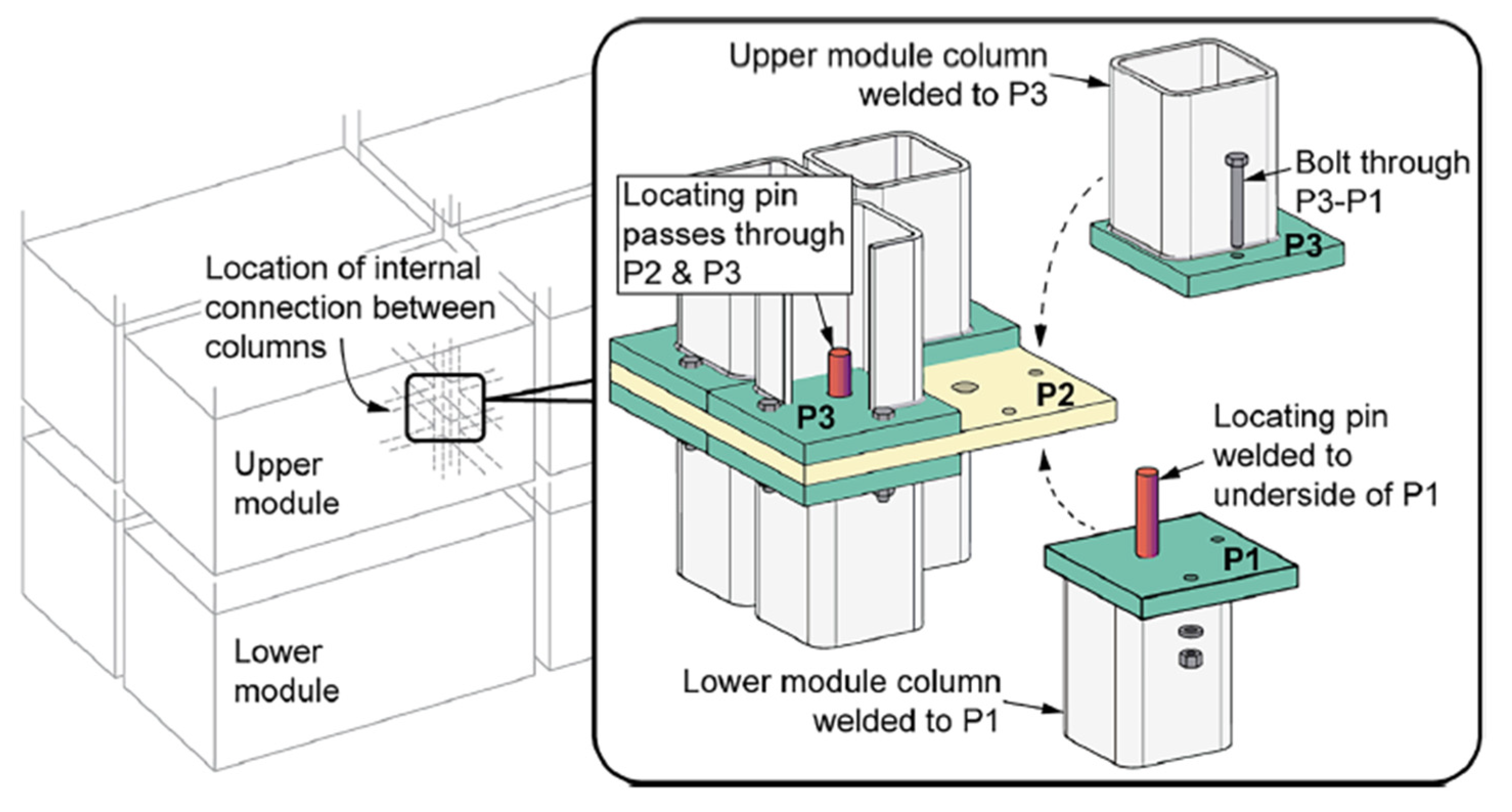
21] introduced an adapted connection that combined blot-and-plate connections with the interlocking action of pins, as shown in
Figure 2. In contrast, the pre-welded locating pins improved the site installation of units; significant slippage was inflicted upon the connection due to the manufacturing tolerances in the blot and pin holes.
The interlocking mechanism allows for quicker assembly and disassembly of modules, which is crucial for modular buildings. Also, those connections can provide significant strength and stability, disturbing loads effectively across the structures as they are fabricated with high precision. Interlocking (IMCs) can accommodate manufacturing tolerances, ensuring a tight and secure fit between the modules; interlocking designs may reduce the need for welding on-site, thereby reducing construction time, labour costs, and potential points of weakness, as it ensures a tight fit between the modules, it can be designed to be visually appealing or completely hidden, maintaining the architectural integrity of the modular building [
19,
21,
54]. The ease of disassembly and reassembly support the rescue of modules in different configurations or locations, aligning with sustainable construction practices by reducing waste and demand for new materials. Yet they raise questions regarding the accommodation of installation tolerances without compressing the slip (deformation) precautions [
21,
49]. This ambiguity underscores the importance of further research in this area; in this context, the plate thickness in interlocking (IMCs) is pivotal and significantly affects the overall structural performance.
Typically, inter-module connections are investigated using experimental programmes, and their outcomes are verified using analytical and numerical research [
21,
38,
55,
56,
57,
58,
59,
60,
61,
62,
63,
64]. The only approaches that can be used to investigate the impact of the interlocking (IMCs) plate thickness are experimental programmers and numerical simulation using the FE methods [
65,
66,
67,
68,
69]. Those approaches have not addressed the optimum plate thickness for interlocking (IMCs) well. With a reasonable material model and effective modelling techniques, the FE method has emerged as the primary analysis tool for predicting the behaviour of inter-module connections (IMCs) under various loading conditions.
To overcome the drawbacks of investigating the optimum interlocking inter-module connections (IMCs) plate thickness, comprehensive research on the analysis of plate thickness and structural integrity of interlocking (IMCs) was conducted in this work since the FE model is cost-effective than experimental programmes, a FE model built upon the work of Lacy et al. [
21] their connection was made up of a three plate (SP14, SP15, and SP16) with a constant plates thickness of 8 mm adapted in this study as the controlled model (A
0). Non-linear analysis was conducted on the proposed four connection models with various plate thicknesses of 4,6,10,12 mm by re-applying the same compression loading AGS-300kNX Universal Test Machine (UTM) conditions of their practical experiment in ANSYS 2023R2 software. Further, the connection stiffness behaviour was addressed in this study. The FE models were then used as the foundation for a comprehensive parametric analysis using MATLAB R2022b to evaluate the slip phenomenal occurrence in the connection using a variety of study approaches, such as polynomial formulas, introduce a slip (deformation) prediction model and validate it with the previous study empirical data, introduce innovative static and machine learning using a ‘Treebagger’ function to train a random forest regression model for predicting slip value based on applied force, and sensitivity analysis study involves multiple steps, including checking error and anomalies and comparing the results with alternative (linear regression analysis and anomaly detection) methods.
2. Modelling Methods
2.1. Connection Configuration and Properties
Inter-module connections are critical because they maintain the modular building’s structural robustness and general stability [
10,
70]. Similarly to Lacy et al.’s [
21] work, the plates are labelled (SP14, SP15, and SP16) for convenience in the following discussion where (SP) refers to
Single
Plate, (t) and (b) refers to the
top and
bottom of the assembled specimen. Their study selected sample (A) as the control model for this study and labelled it as (A
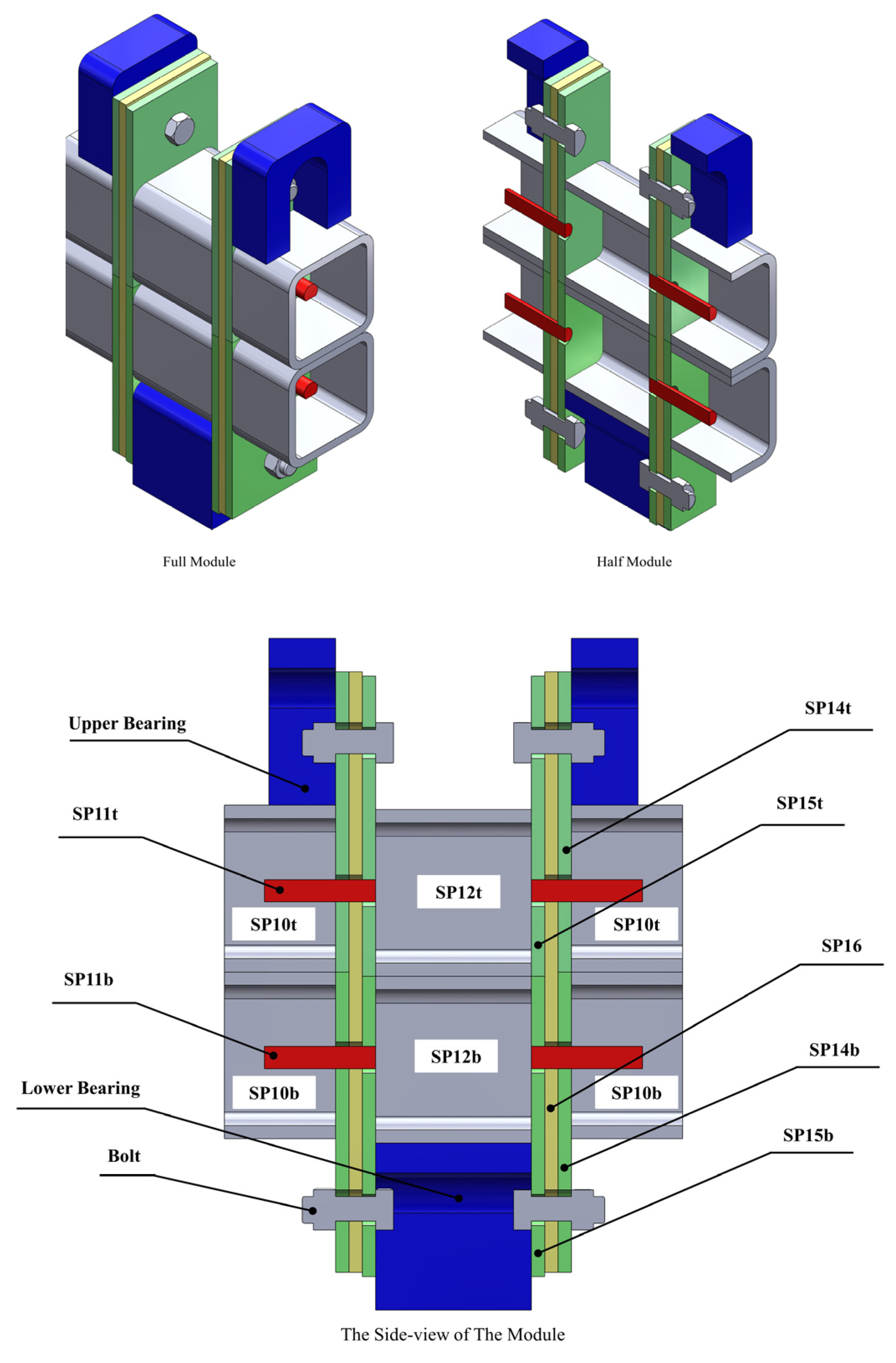
0). The connection design focused on the interplay between (SP14, SP15, and SP16); the connection geometry shown in
Figure 3 captures the full and cut-way view to present the hidden connection components and the connection dimensions specified in
Table 1.
The material properties of the connection are selected to meet stringent industry standards, emphasising specific criteria for strength and durability, as shown in
Table 2. The variations in the connection plate thickness are shown in
Table 3. Each plate type was evaluated through a series of cases starting with (A
0) representing the controller model, (A
1) to (A
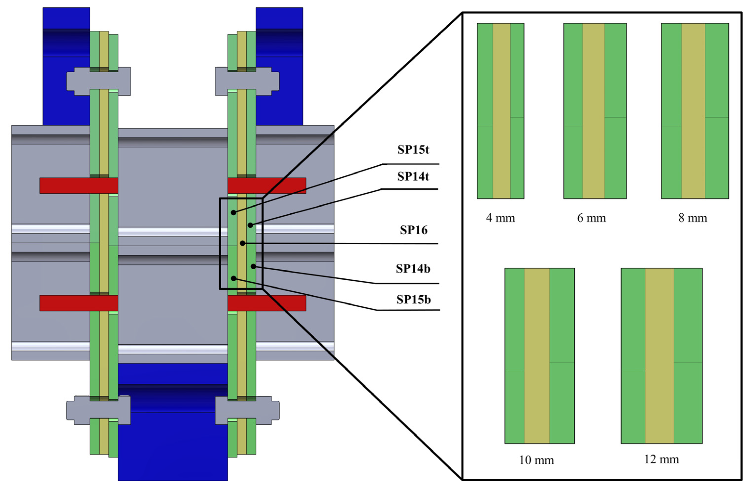
4) presenting the proposed cases, with interlocking (IMC) plate thickness ranging from 4.0 mm to 12.0 mm, as shown in
Figure 4.
2.2. Compression Loading (UTM) Test Conditions Modelling
To re-apply the same compression loading AGS-300kNX Universal Test Machine (UTM) conditions of practical experience in ANSYS 2023R2 software, an FE method was adopted. In the previous study, Lacy et al.’s [
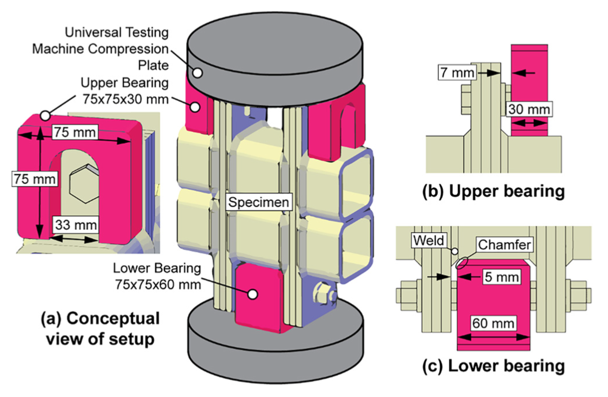
21] sample (A) was modelled using ABAQUS software by applying (UTM) test loading conditions with loads ranging from 0 to 250 kN at a rate of 0.1 kN/s (refer to
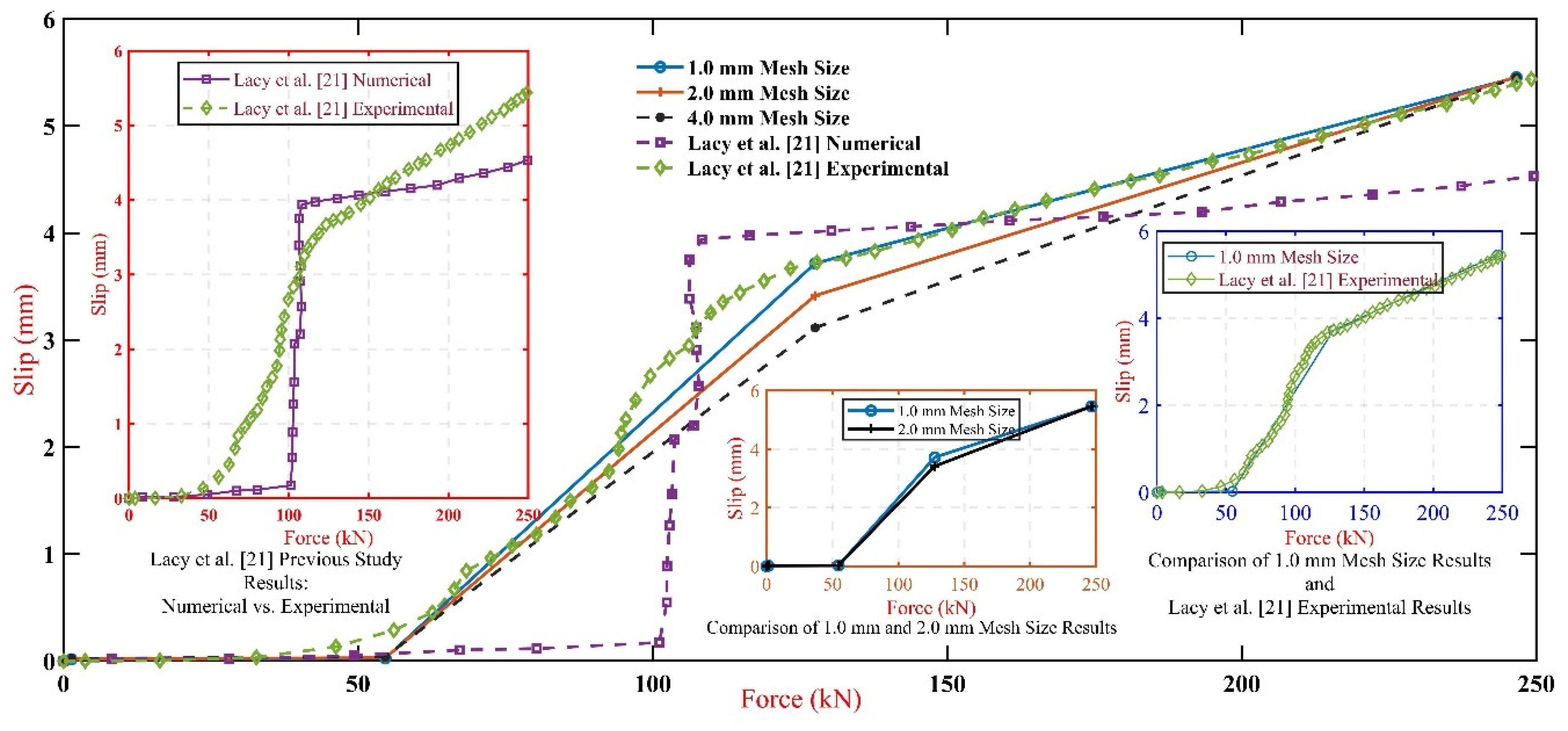
Figure 5) the previous FE model was employed 8-node linear brick elements with reduced integration (CSD8R). However, the validation error between their numerical and experimental results was over 95.62%, as shown in
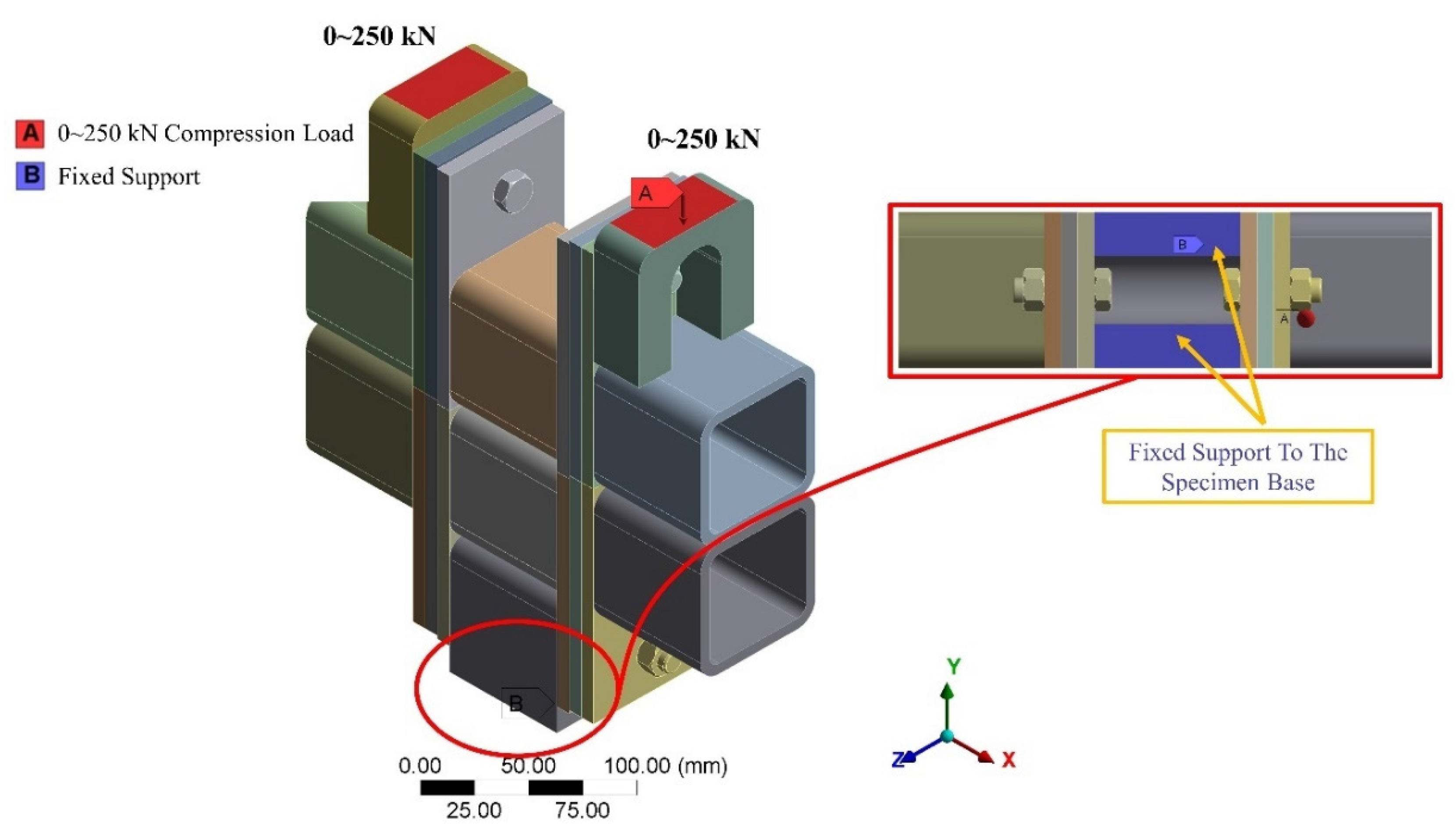
Figure 8. Therefore, this study remodels the actual experimental test by re-applying the same compression loading AGS-300kNX Universal Test Machine (UTM) conditions of their practical experiment in ANSYS 2023R2 software, as shown in
Figure 6 by applying a compression load with a load range of (0~250kN) in negative Y-axis direction, and fixed support to the specimen base.
2.3. Interlocking Connection Modelling
To investigate the accuracy of the optimum interlocking (IMCs) plate thickness numerically, FE models with various plate thicknesses of 4, 6, 10, and 12mm (refer to
Table 3) were developed in ANSYS 2023R2 as shown in
Figure 4 based on the experimental approach presented by Lacy et al. [
21]. The geometric properties of the connection cases were defined in the FE model following
Table 1 and their materials specifications were defined following
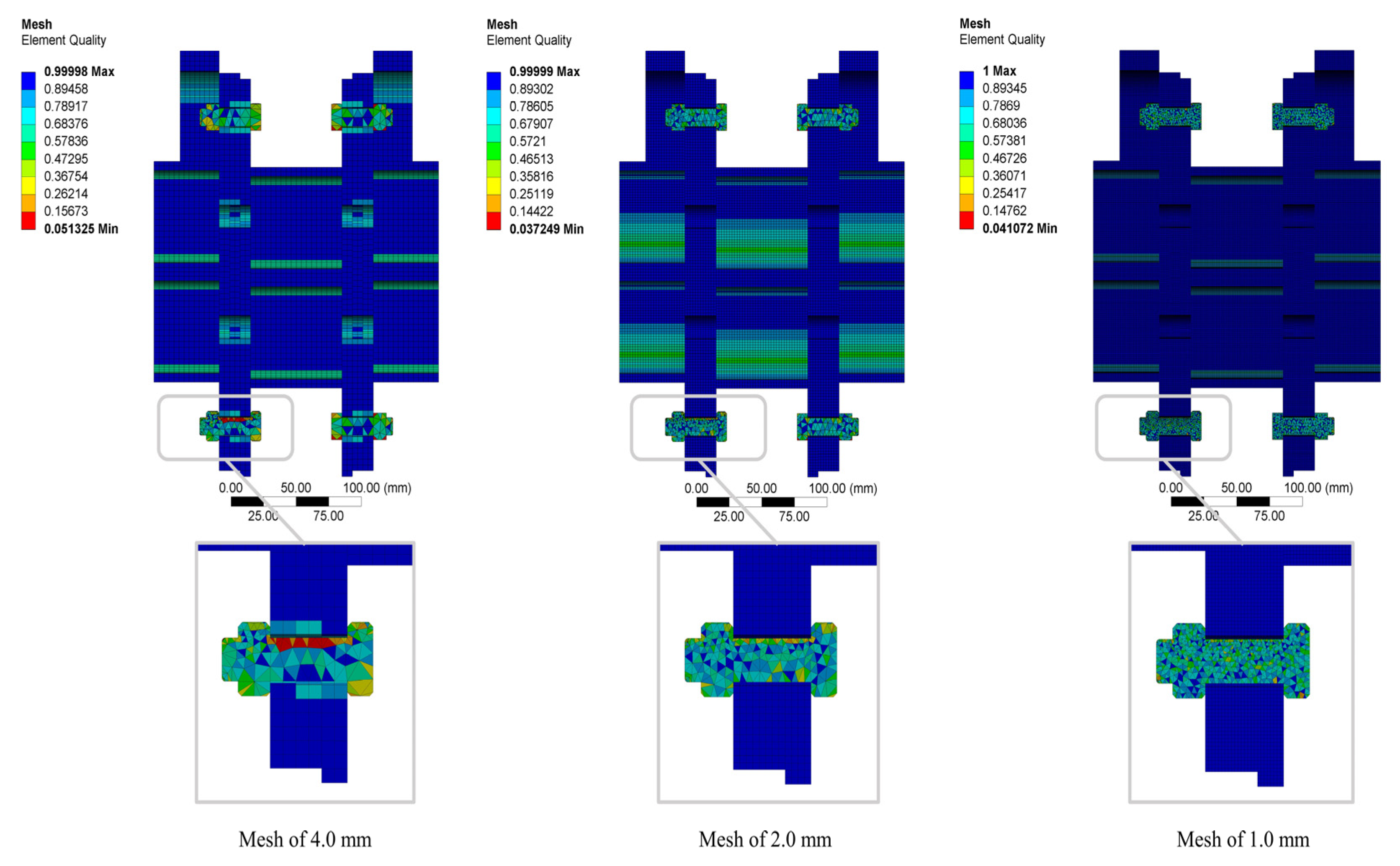
Table 2. The models were subjected to a selected mesh elements size of 1.0 and 2.0. and 4.0mm with a growth rate set at 1.2. To balance an accurate and efficient FE model, a middle range of detail (coarse) at the centre of the span angle, added initial size seeds to the assembly, and the error limits to be more aggressive, allowing for a maximum of five mesh layers as shown in
Figure 7, a mesh size of 1.0 mm reaches the maximum mesh quality of 25.31% compared to 2.0 and 4.0mm. To validate the accuracy of the FE model,
Figure 8 shows the comparative analysis between force-slip Lacy et al. [
21] experimental approach results and FE model mesh sizes results; validation results reveal that the validation error between the FE model results and the experimental results was 2.13%, which more accurate 95.63% than the previous study FE results, this study therefore adopted 1.0m elements mesh size though all the FE modelling.
Figure 7.
FE model (1.0, 2.0, and 4.0mm) mesh size.
Figure 7.
FE model (1.0, 2.0, and 4.0mm) mesh size.
Figure 8.
Comparative analysis between force-slip Lacy et al. [
21] experimental approach results and FE model mesh sizes results.
Figure 8.
Comparative analysis between force-slip Lacy et al. [
21] experimental approach results and FE model mesh sizes results.
3. FE Results & Discussion
3.1. Slip (Deformation) Behaviour
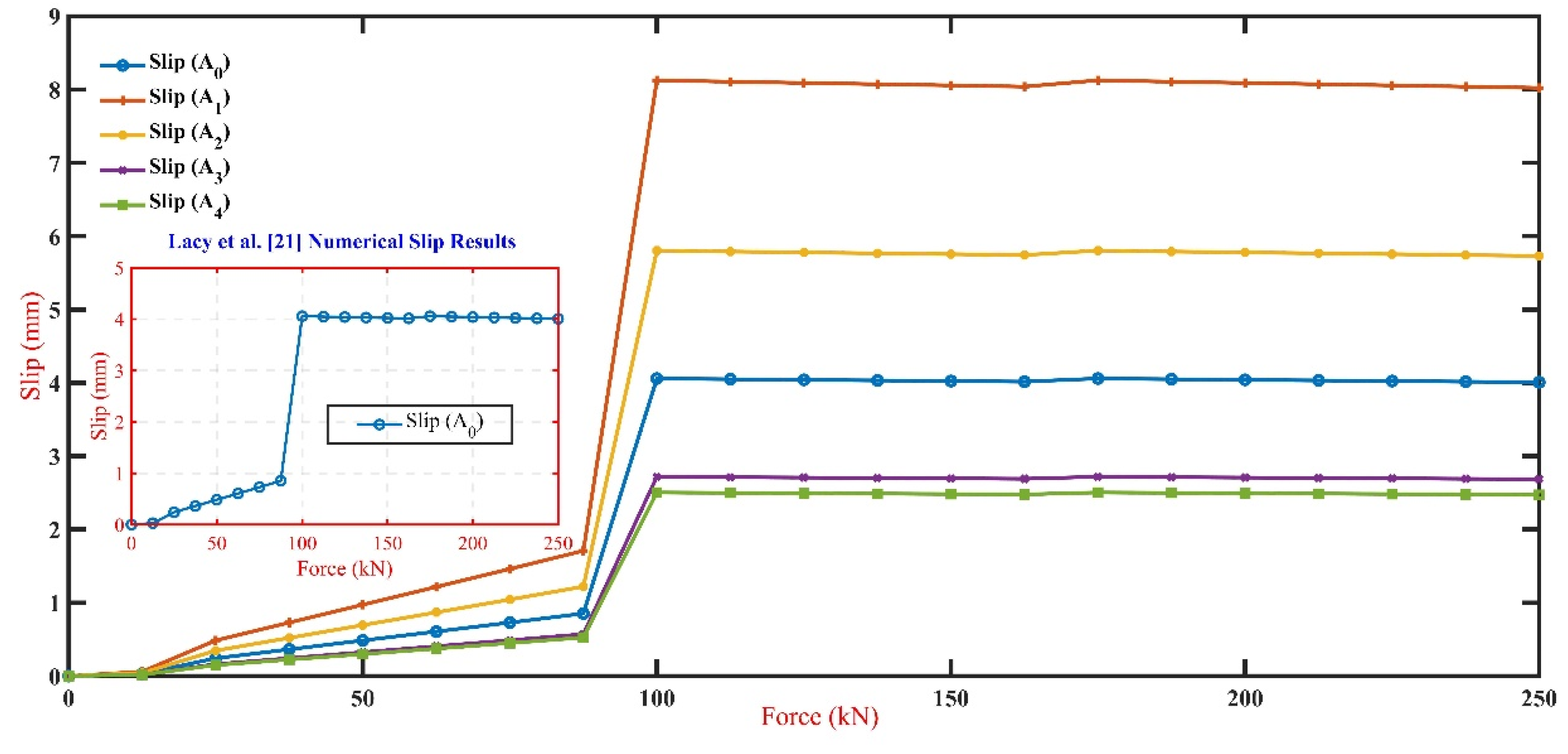
The examined slip (deformation) across the interlocking inter-module connections (IMCs) plat thickness scenarios (A
0 through A
4) are shown in
Figure 9. The analysis reveals that the controller model (A
0) exhibits an increased slip with the applied force, reaching a slip of 4.0mm at 250kN. Notably, compared to case (A
1), which exhibits a slip increase peaks up to 8.02mm at the same applied force, emphasising the heightened susceptibility to slip in thinner plates. Case (A
2), with an intermediate plate thickness, shows an elevated slip behaviour less than (A
1). (A
3) and (A
4) cases demonstrated a notable reduction in slip, with (A
4), the thickest plate, exhibiting a 2.46mm slip at 250kN force, which has a reduction of (≈38%) from the controlled model (A
0).
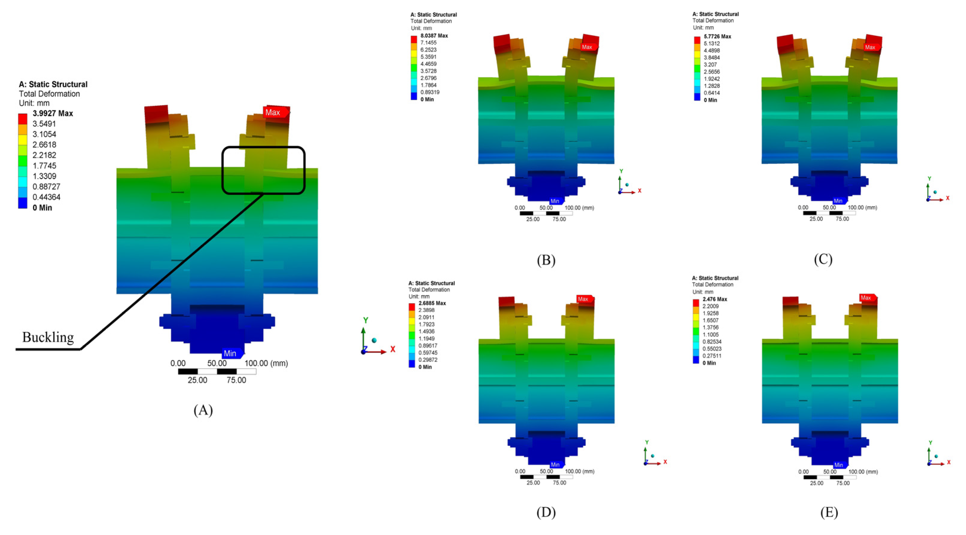
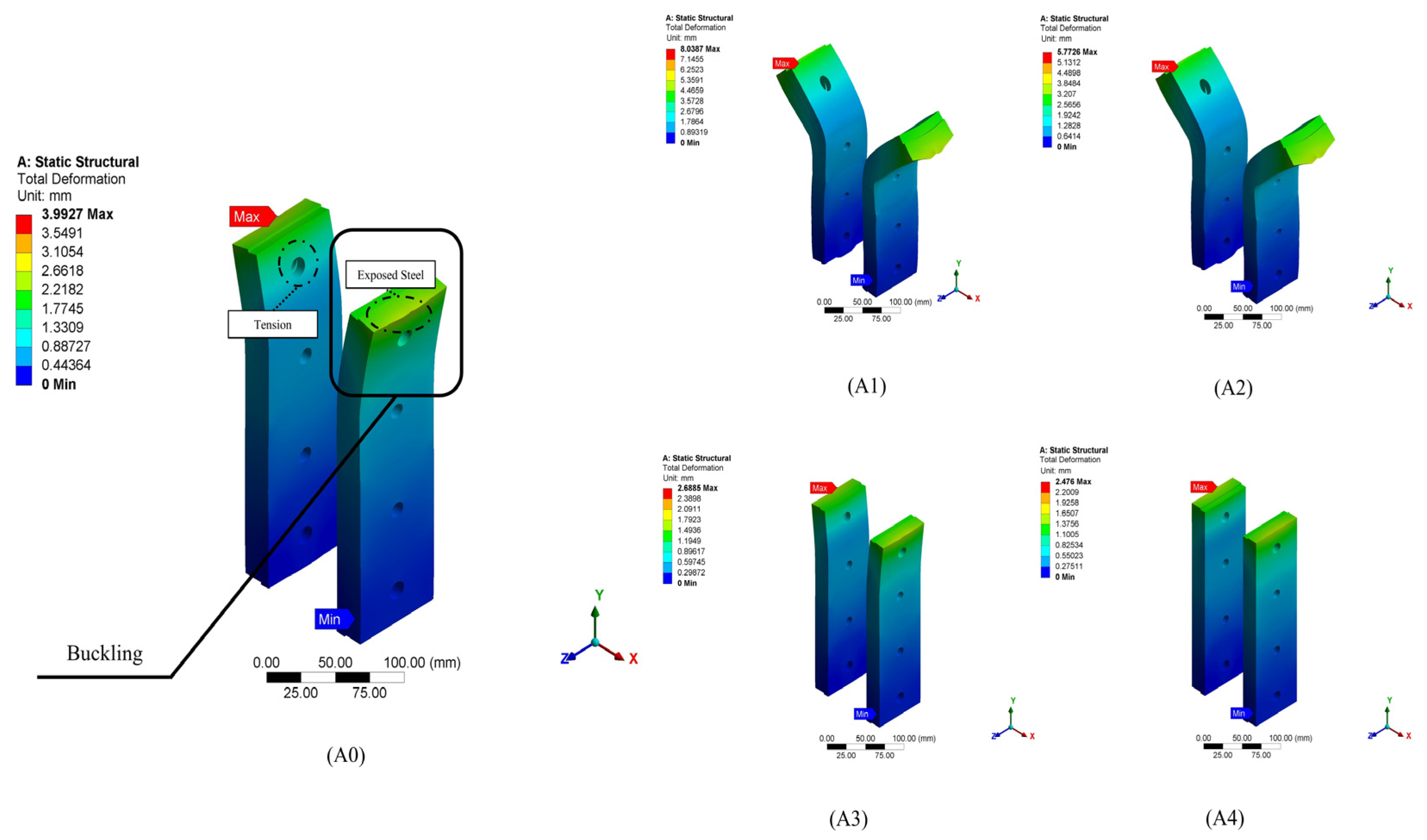
The deformation and buckling in the connection’s cases of the varying plate thickness and their impact on the connection stability are shown in
Figure 10. The controlled model (A
0) showed mid-plate buckling, particularly in the 8mm (SP14) plate top and bottom regain, tension at the upper bolt holes, and steel exposure near the upper bearing, indicating structural vulnerabilities. Halving the thickness to 4mm, as in case (A
1), exacerbates buckling and tension increase, reflecting the reduced capacity of thinner plates to maintain structural integrity. A moderate improvement is seen in case (A
2), reducing buckling relative to (A
1), but it still suffers from notable tension and buckling, indicating improvement needs. A marked enhancement in the connection resistance is observed in case (A
3), where 10mm plates minimise deformation with a reduction in buckling and tension. The most substantial resistance to buckling is achieved in case (A
4), where the thickest plates exhibit the best minor deformation, minimal buckling, tension, and reduced steel exposure.
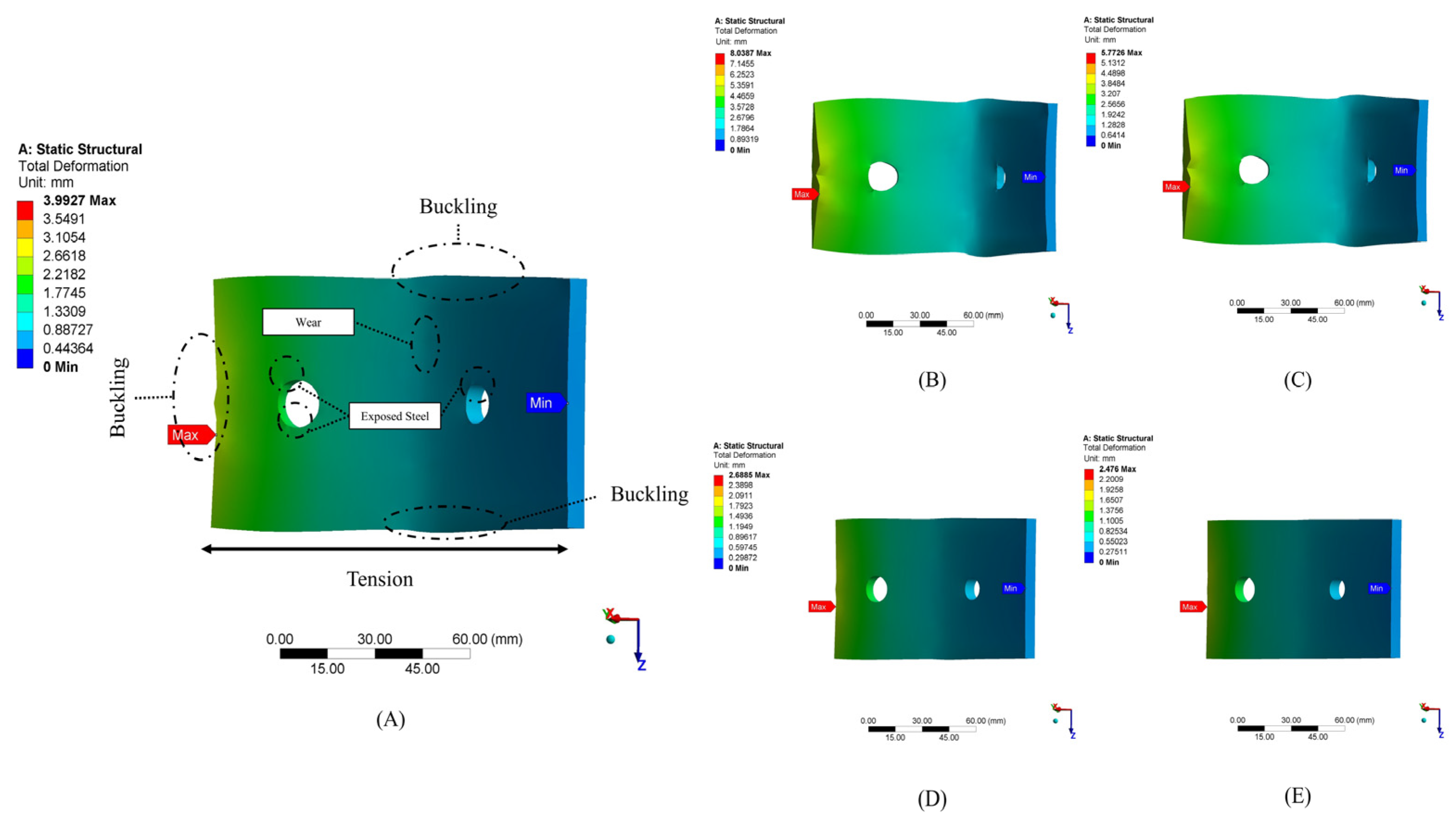
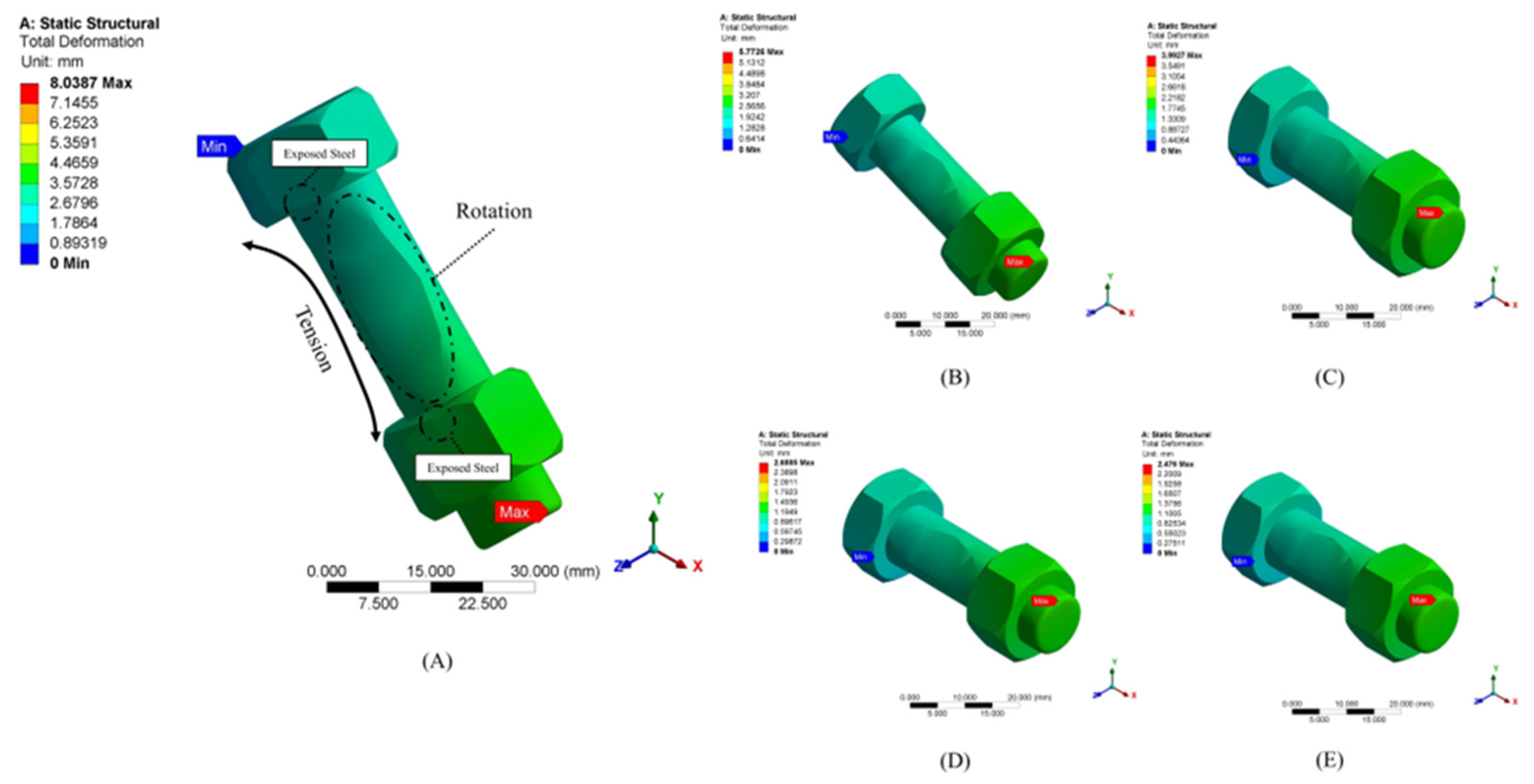
For closer observation of the plate (SP14) and its bolt deformation across the case studies,
Figure 11 shows each case’s failure modes. In the controlled model (A
0), buckling presents at the critical stress point (top, bottom, and corner of the plate) alongside tension across the late near to midsection and exposed steel around the bolt holes. Case (A
1) present the severe plate failure scenario with significant steel exposed at both the bottom of the head and the top of the bolt nut. Case (A
2) shows a partial recovery from (A
1). With plate buckling reduction, however, the plate exhibits considerable tension and exposed steel with tension and rotation alongside the bolt body. The failure modes improved in case (A
3); buckling, tension, wear, and exposed steel are significantly diminished in the plate, suggesting a more resilient connection that can better handle the stress applied to the bolts. Case (A
4) starts the optimal structural behaviour with minimal buckling, negligible wear, reduced tension, very little exposed steel, and a minor bolt deformation, indicating the most robust connection among all cases. Therefore, it was concluded that the increased plate thickness correlates with enhanced interlocking (IMCs) stability.
3.2. Stability and Stiffness Behaviour
Stiffness measurements investigated the stability and stiffness of the connection configurations across the case studies (A
1 to A
4) compared to the controlled model (A
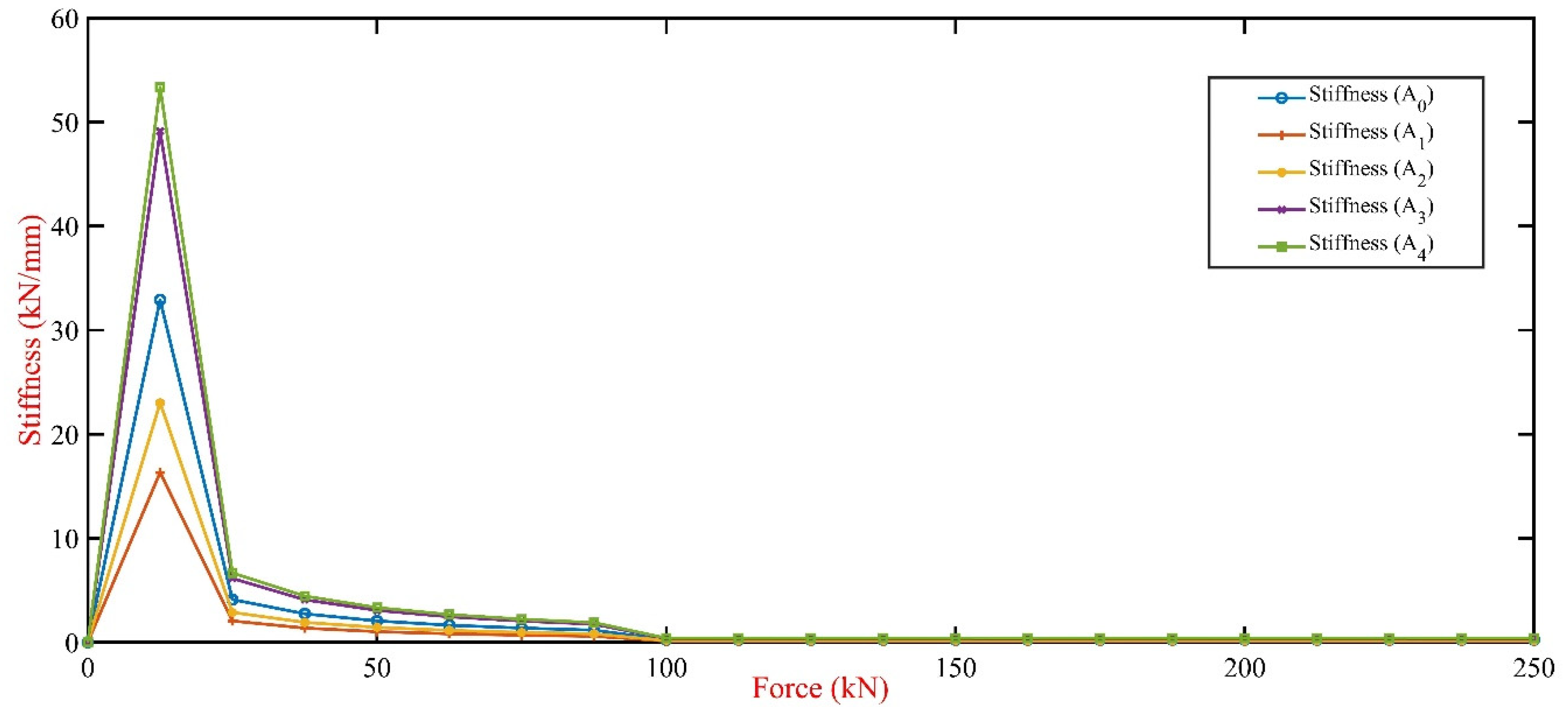
0), as illustrated in
Figure 12. The investigation reveals that the control model (A
0) stiffness consistently maintained zero values, indicating no additional stiffness contribution. Notably, case (A
4) stiffness demonstrated the highest stiffness values, reaching a peak of 53.33kNa/mm at 12.5 kN force, 62.07% higher than the controlled model (A
0) stiffness at the same point force and 50.75% lower than case (A
3). The lowest stiffness values were recorded in case (A
1) with a significant decrease to 2.05kN/mm at 25kN point force. This highlights the substantial impact of interlocking (IMCs) plate thickness on the structural integrity of MSBs, with thicker plates markedly enhancing stability and stiffness, potentially offering improved deformation resistance and overall structural robustness.
4. Advanced Predictive Modelling Study
4.1. Polynomial Regression Formula and R-Values
In MSBs, optimising interlocking (IMCs) through precise plate thickness selection is a cornerstone for enhancing MSB’s structural integrity. Polynomial formulas for predicting slip (deformation) were derived by considering the connection plate thickness variations across five distinct models, (A
0) through (A
4). The accuracy of these predictive models is quantified by their respective R-values, indicating the strength and reliability of fit to the observed data. Based on Lacy et al.’s [
21] empirical data and using a cubic polynomial fit, the derived polynomial regression formula for slip (
∆) for the control model (A
0) and its R
2 value are as follows.
where in Equation (1)
F is the applied force, and the R
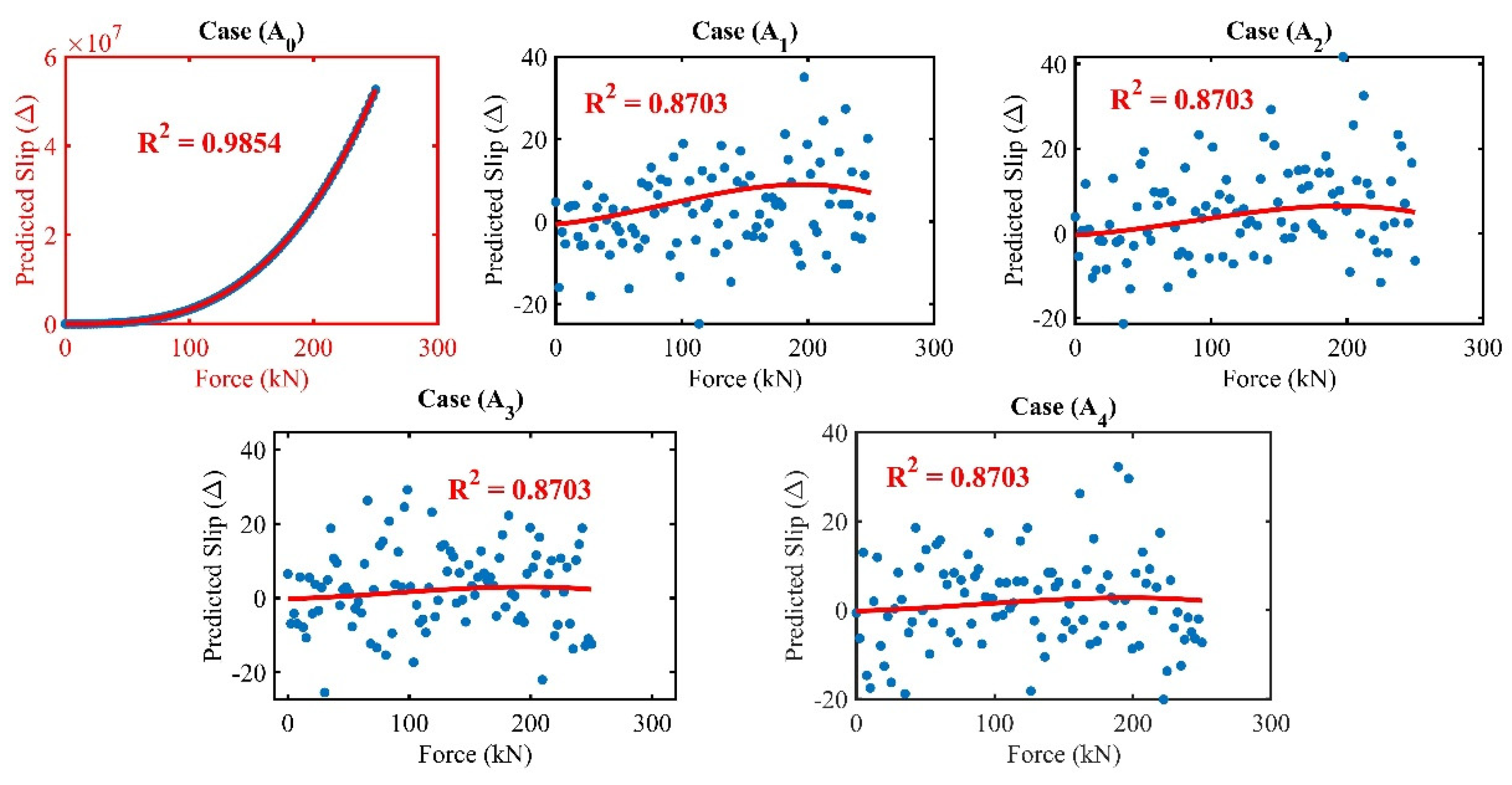
2 value is 0.9854, as shown in
Figure 13. following the cubic polynomial fit approach, the remaining cases (A
1 through A
4) formulas are as follows.
In those cases, polynomial regression formulas represent R
2 values of 0.8703, as shown in
Figure 13.
4.2. Polynomial Regression Model for Slip Prediction
The development and application of a polynomial regression model designed to predict slip phenomena (
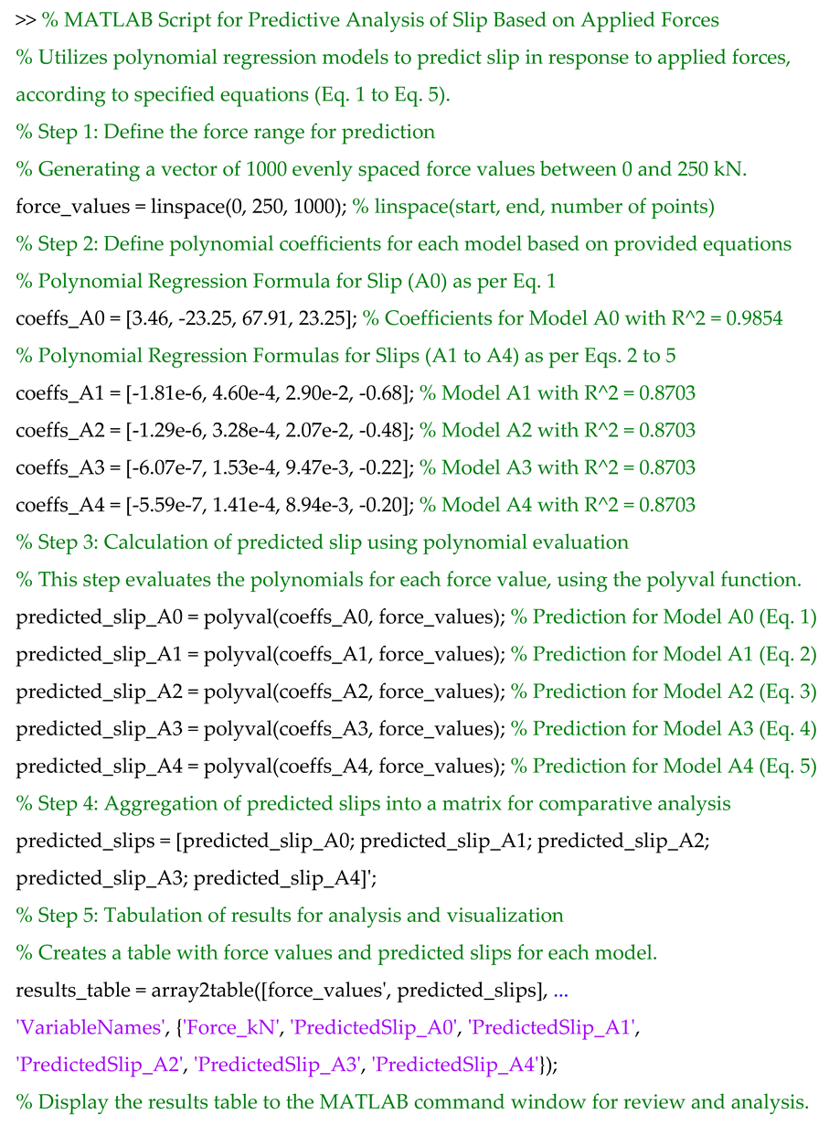
∆) in response to a range of applied forces (0 to 250 kN). This model (refer to
Appendix A) is central to understanding the intricate non-linear relationships between the forces applied to interlocking mechanisms and the observed slip responses. It is represented mathematically as:
Equation (6) captures the essence of the slip prediction model, where (∆) denotes the slip, (F) represents the applied force, and (an) through (a0) are the coefficients that define the curve’s shape based on the degree (n) of the polynomial. These coefficients are critical as they embody the model’s sensitivity to changes in force, enabling the prediction slope with varying degrees of applied forces. The development and implementation of this model were carried out in MALATAB R2022b. This included generating a comprehensive set of force values within the specified range and applying the polynomial coefficients to predict slip outcomes. The process began by defining a vector encompassing 1000 evenly spaced force values between 0 and 250 kN to cover a broad spectrum of potential scenarios. Specific polynomial coefficients were established based on predefined equations for each model variant (A0 through A4). These coefficients are instrumental in delineating the model’s predictive accuracy and were selected to closely mimic the empirical data observed in slip phenomena. Using MALATAB R2022b’s ‘polyval’ function, the polynomial equations were evaluated for each force value, facilitating the slip prediction across the range of applied forces. This pivotal step transforms theoretical constructs into practical, predictive insights that accurately reflect the slip behaviour under various force conditions.
4.3. Validation of Polynomial Regression Model
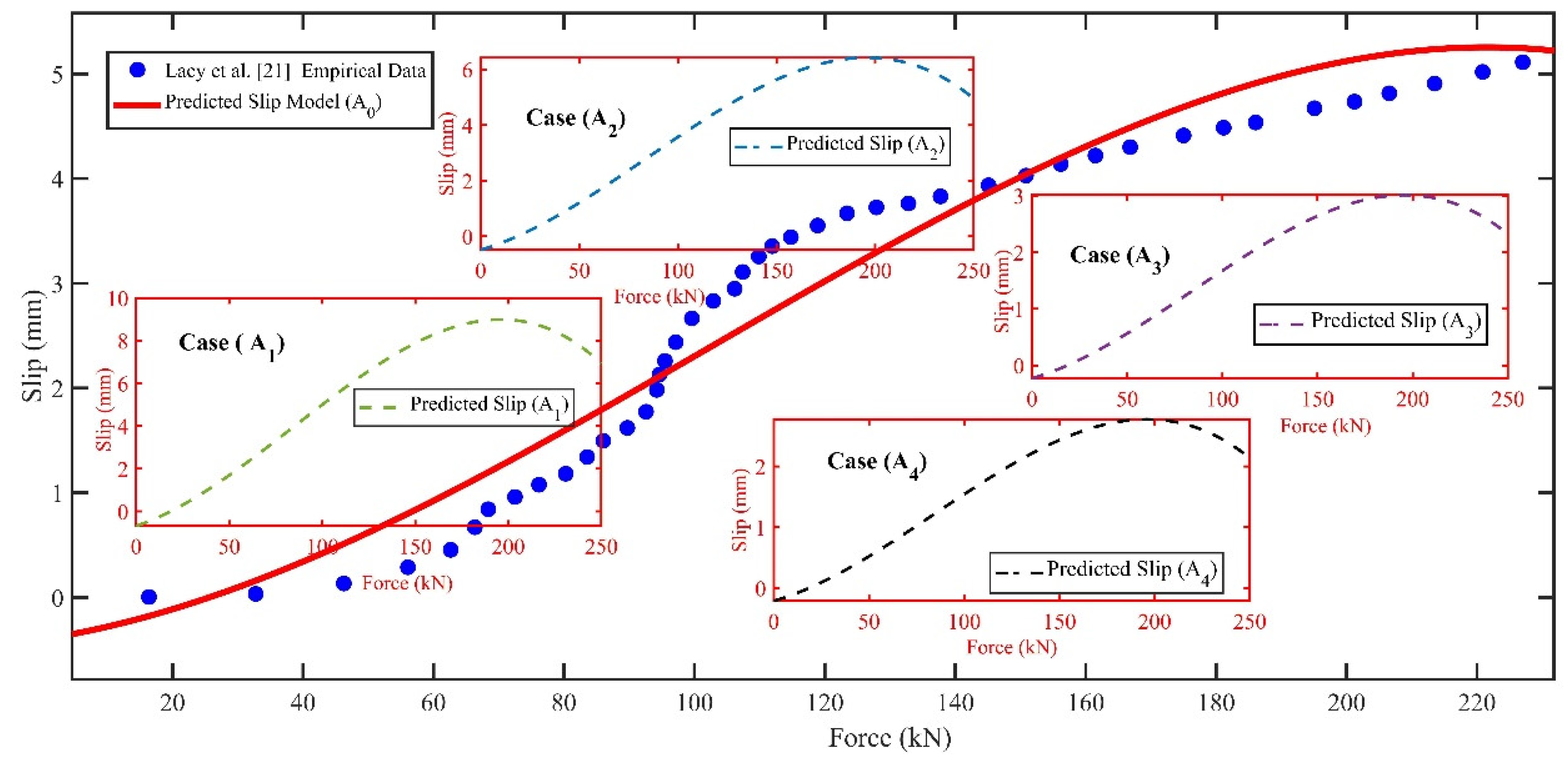
The polynomial regression model, specifically the control model (A
0), was validated by comparing its predictions against empirical data from Lacy et al.’s [
21] experiments, as depicted in
Figure 14. This comparison evaluated the model’s precision in predicting slip due to varying applied forces, employing MALATAB R2022b for the analytical process. The evaluation revealed a range of accuracy in the model’s predictions. On one end, some predictions showcased exceptional accuracy, with errors as low as 0.11%. Conversely, the model’s predictions diverged significantly from the experimental data at higher slip values, with errors reaching up to 24.16%. This variability highlights the model’s fluctuating accuracy across different force levels.
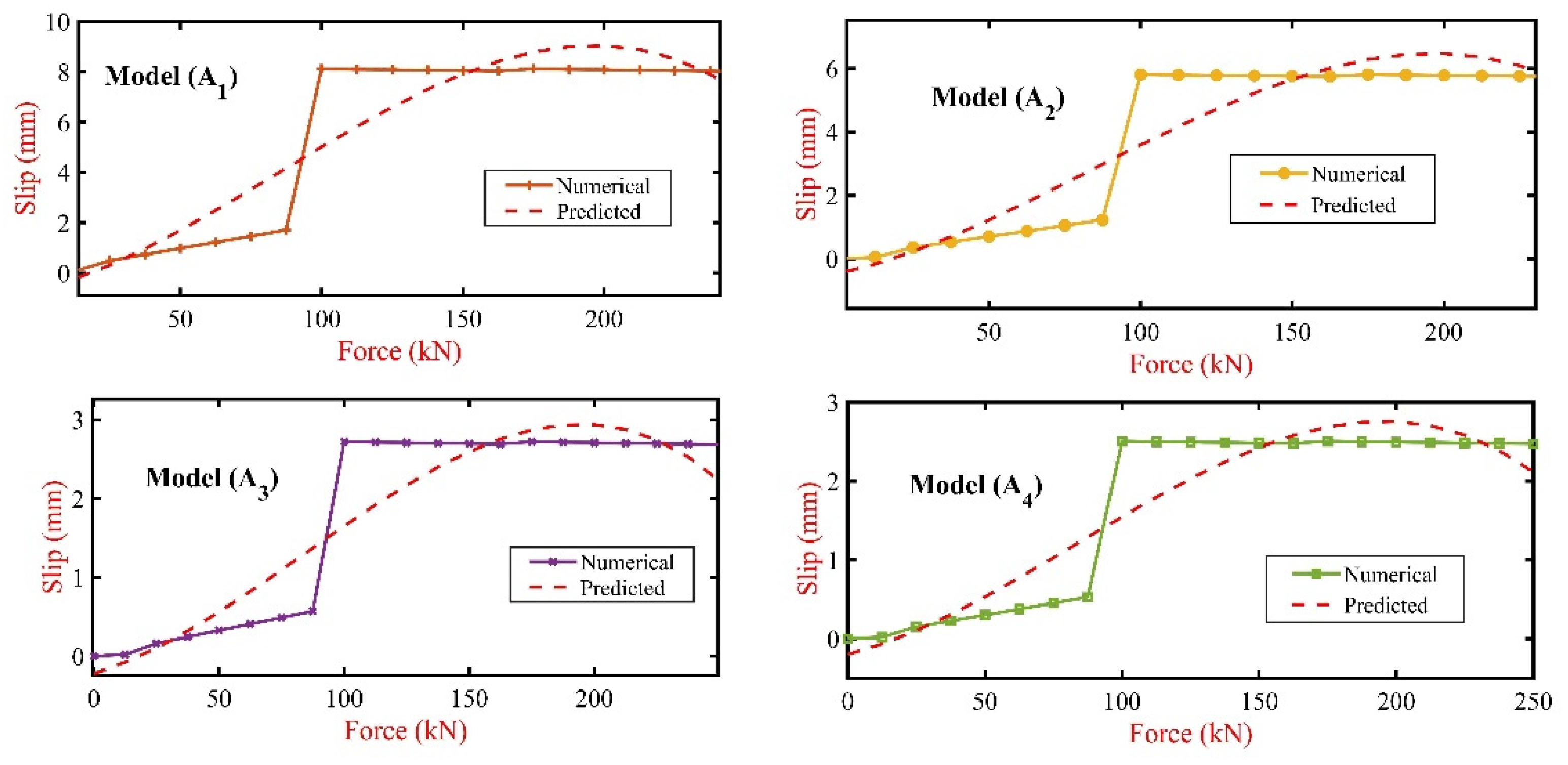
A comprehensive analysis was conducted to quantify the overall performance of the model. The total absolute difference between the model’s predictions and the empirical slip values was approximately 16.30 mm, calculated across all data points, excluding zero slip scenarios, for greater precision. This resulted in an average error rate of approximately 10.80%, indicating a generally commendable level of accuracy in the model’s slip predictions. Further comparisons involved the model’s performance against Finite Element (FE) models (A
1) through (A
4), as detailed in
Figure 15. These comparisons revealed varying degrees of accuracy, with the model (A
1) exhibiting an average error of about 59.50%, indicating a significant deviation from actual slip values. Models (A
2) and (A
3) showed slightly better but still considerable error rates of 59.10% and 57.90%, respectively, while model (A
4) emerged as the most accurate, with an error rate of approximately 57%. These results underscore the challenges in slip prediction and highlight the potential for refinement in the polynomial regression model’s application.
4.4. Machine Learning Model Analysis
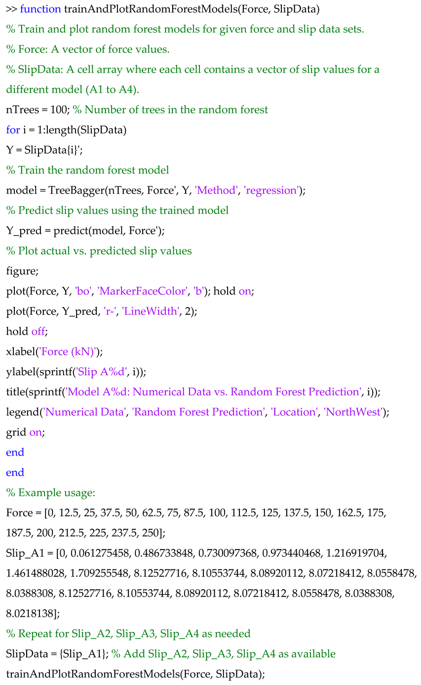
The previous validation approach affirms the model’s efficiency in predicting slip across forces range and highlights potential avenues for further refinement. This study delves into deploying a machine-learning model (refer to
Appendix B) using the MATLAB R2022b ‘TreeBagger’ function to enhance slip prediction accuracy across various forces. The ‘TreeBagger’ tool employs a random forest regression approach, an ensemble learning method that constructs multiple decision trees during the training phase. This method is renowned for its robustness and flexibility in modelling complex, non-linear relationships without a predefined model structure. Utilising this approach, the study iterated over four sets of slip data (A
1 to A
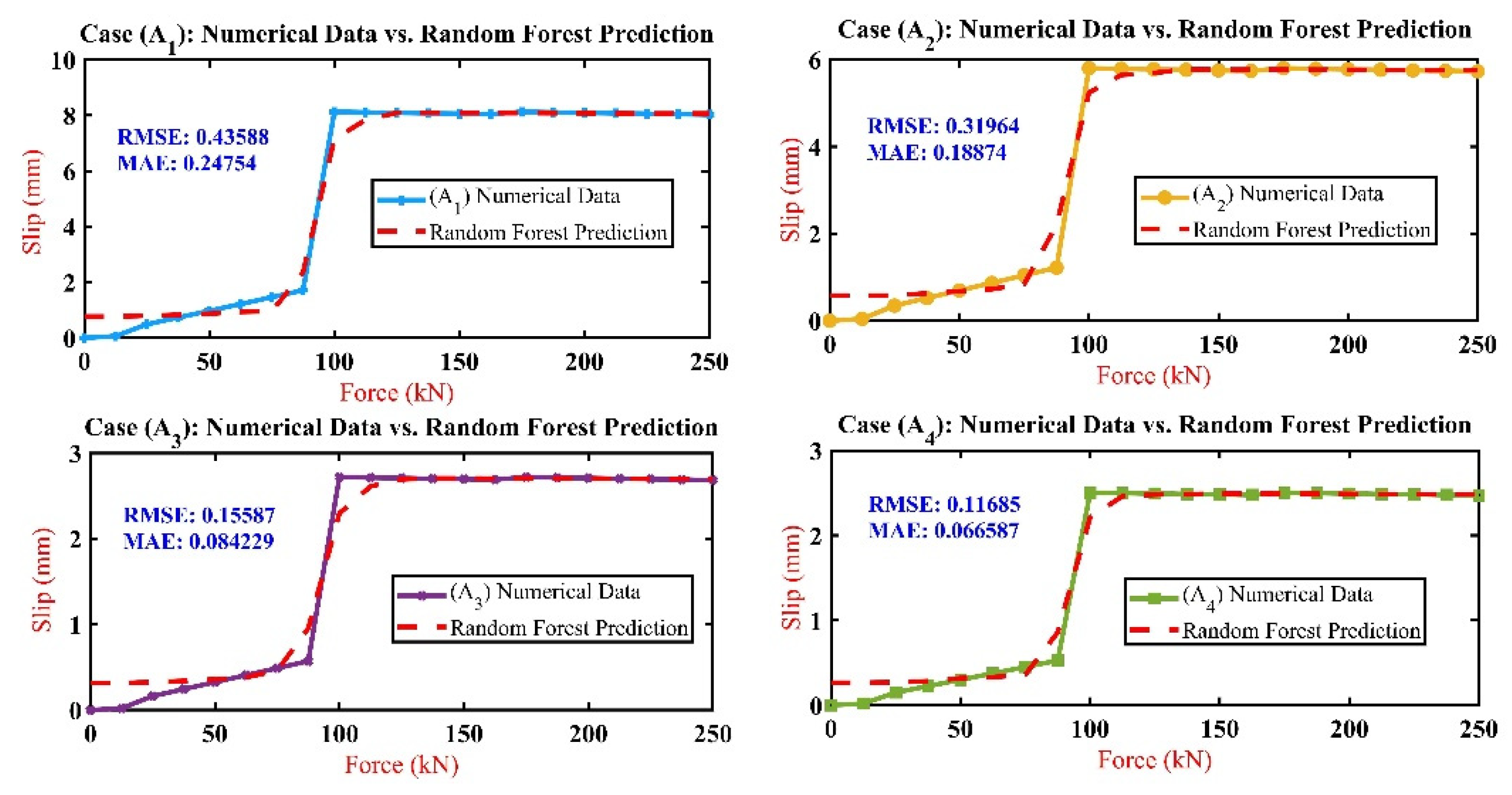
4), each employing the applied force as the predictor variable and the corresponding slip values as the response variable. The model was trained for each dataset and subsequently used to predict slip values, plotted against actual data for a visual comparison. Two key metrics were employed to quantify the model’s predictive performance: Mean Absolute Error (MAE) and Root Mean Square Error (RMSE). MAE calculates the average absolute differences between the predicted and actual values, offering a measure resistant to outliers. Conversely, RMSE provides the square root of the average squared differences between predicted and actual values, offering insight into the overall magnitude of the prediction error. A comparative analysis of the model’s performance across the datasets (A
1 to A
4) revealed that case (A
4) exhibited the most favourable outcomes in terms of both RMSE and MAE. This indicates that (A
4) had the lowest average error magnitude and demonstrated the highest resilience against outliers. Following (A
4), the models’ performance in terms of accuracy improved progressively from (A
3) to (A
2) and lastly to (A
1), as detailed in the results shown in
Figure 16. The analysis highlighted a notable overestimation in initial slip predictions for lower forces (0 to 75kN). However, the model’s predictions for higher forces (above 87.5kN) closely matched the empirical slip values. For instance, at a force level of 100kN, the maximum deviation observed was approximately 7%, with the numerical slip at 8.1253mm and the random forest’s prediction at 7.193mm for case (A
1). In contrast, for cases (A
2) and (A
3), the predicted slip values were lower by approximately 11.70% compared to the empirical values at the same force level. In contrast, case (A
4) exhibited a slight discrepancy of about 14.80%. In conclusion, the machine learning analysis, powered by ‘TreeBagger’, underscores the effectiveness of the random forest model in predicting slip across varying forces. This approach highlights the model’s strengths and its potential areas for improvement. The observed trend, starting with an overestimation at lower forces and achieving higher accuracy at greater forces, signals a promising direction towards refining the accuracy of interlocking mechanisms’ models.
5. Advanced Predictive Modelling Study
This study delves into the impact of plate thickness variations on the stiffness characteristics (ranging from stiffness A0 to stiffness A4) of interlocking inter-module connections (IMCs) in Modular Steel Buildings (MSBs). The core of our analysis involves utilising MATLAB R2022b to conduct a detailed sensitivity analysis, focusing specifically on how changes in applied force influence the stiffness attributes. This involves assessing the rate of stiffness changes to applied force, highlighting the relationship between force fluctuations and stiffness response. The sensitivity analysis using MATLAB R2022b involved (1) checking for errors and anomalies and (2) comparing the sensitivity results with alternative methods (linear regression analysis and anomaly detection).
5.1. Stiffness Sensitivity Analysis
This study delves into the intricacies of how variations in plate thickness influence the stiffness attributes (stiffness A
0 to stiffness A
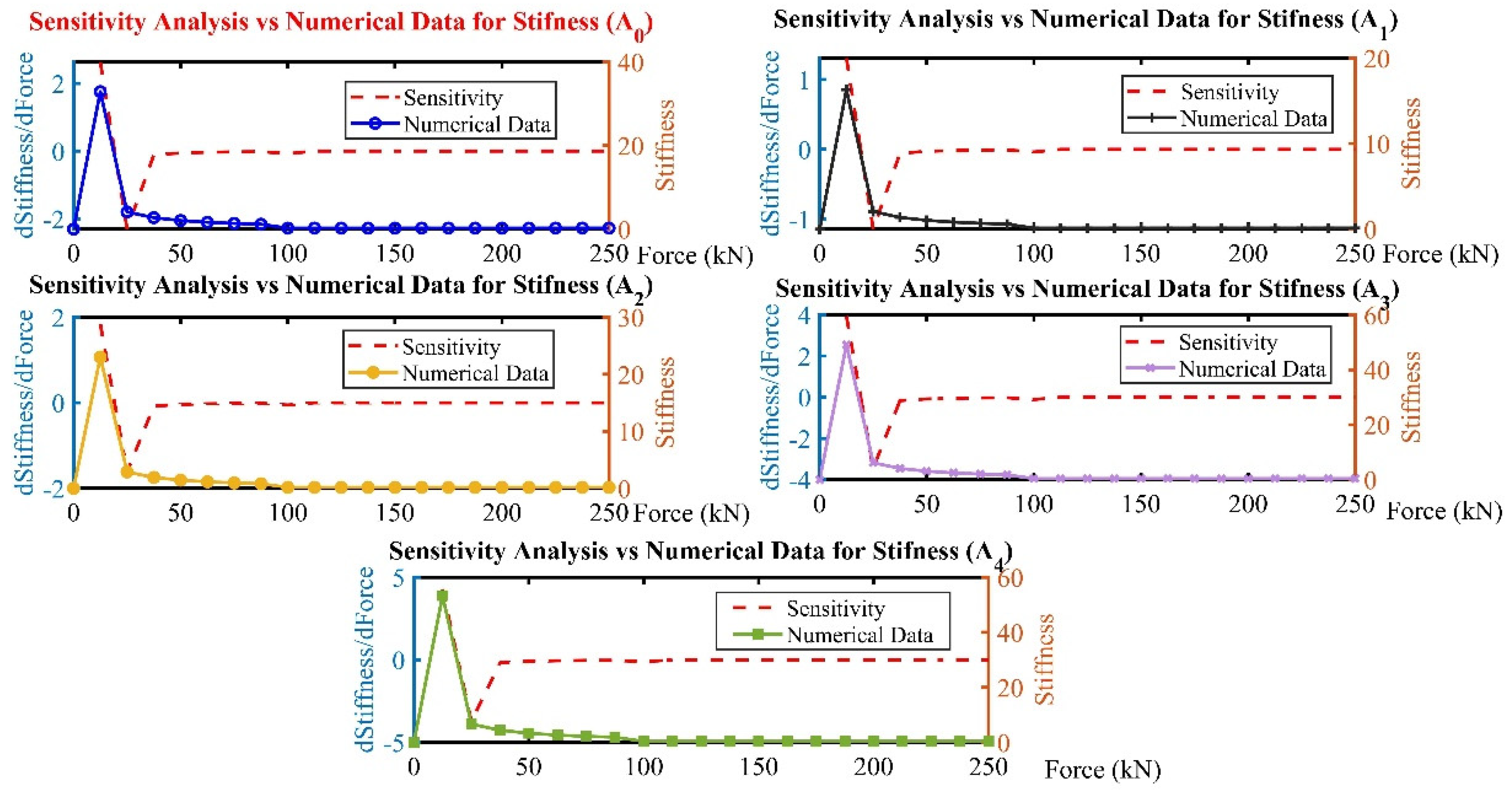
4) within interlocking inter-module connections (IMCs) for Modular Steel Buildings (MSBs). Employing MATLAB R2022b for comprehensive sensitivity analysis, this segment evaluates the derivatives of stiffness in relation to applied force across different attributes, delineating their sensitivity to force alterations through calculated rate changes and visual comparisons with the numerical stiffness metrics. The analytical process unfolds in the following manner: (1) dataset definition, (2) rate of change calculation (derivative), and (3) results visualisation, where the rates of change are plotted alongside the numerical stiffness, as shown in
Figure 17.
The insights from this analysis are systematically compiled and presented in
Table 4, which encapsulates the average sensitivity across the stiffness attributes. Furthermore,
Table 4 expands to mapping the sensitivity variability and underscoring the stiffness attribute's differential responsiveness to applied forces. The data reveals a gradation in average sensitivity and stiffness across the attributes. Notably, the controlled model (A
0) showed an average sensitivity and average stiffness of 2.3441, indicating a moderate responsiveness to force changes. In contrast, case (A
1) exhibits the lowest average sensitivity and stiffness (1.1653), suggesting a less pronounced structural response to force variations; case (A
2) shows an average sensitivity and stiffness (1.6392) positioned between model (A
0) and case (A
1), highlighting a balanced approach to stiffness and adaptability. This could imply a strategic design consideration to optimise rigidity and responsiveness to applied forces. The analysis takes a significant turn with the Stiffness case (A
3) and case (A
4), where a marked increase in average sensitivity and stiffness is observed. (A
3), with an average stiffness of 3.4987, alongside case (A
4) leading stiffness of 3.7992, underscores a heightened structural response to force applications. This heightened sensitivity and stiffness might reflect a design optimised for environments demanding high durability and adaptability to varying loads, potentially offering enhanced performance in dynamic or unpredictable conditions.
5.2. Errors and Anomalies
To quantitatively assess the sensitivity of models (A
0 through A
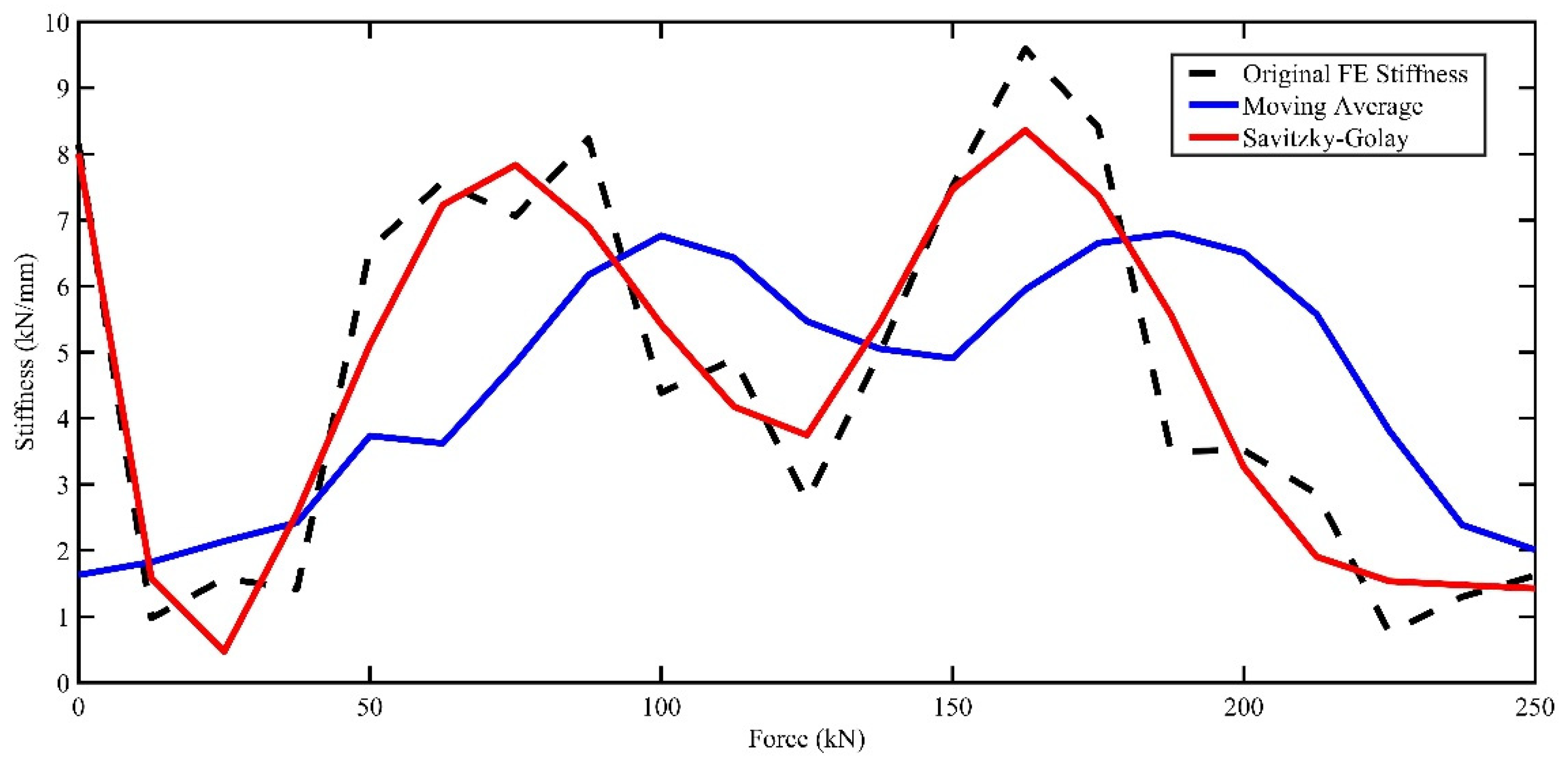
4) stiffnesses to changes in applied loads and detect and highlight the animalise that might indicate data inconsistencies, measurements errors or other noteworthy deviations from expected patterns. Anomalies detected at the initial force indices across all attributes highlight the necessity to refine the analysis techniques. Advanced filtering, expressly, the (Moving Average [
71] and SavitzkyGolay filters [
72]) was incorporated to address these issues. Those methods are proviral in reducing noise and enhancing the signal quality of the stiffness data, which is critical for the accuracy of the predictive models.
Figure 18 presents the variances between the ‘Original FE stiffness’ measurements and those adjusted by ‘Moving Average’ and ‘SavitzkyGolay’ filtering techniques across the force range. The ‘Original’ data exhibits considerable fluctuation, ranging from lows of 0.75 to highs of 9.39, which obscure actual material behaviour under the force’s applications. While smoothing data, the ‘Moving Average’ approach consistently underestimates stiffness at higher force levels. There were discrepancies as stark as a reduction to 1.204 from an original 6.0198 at 0 kN, suggesting an average dampening effect of 79% compared to ‘Original’. Conversely, the ‘SavitzkyGolay’ filter more closely aligns with the ‘Original’ data, retaining essential features such as peaks and troughs, with deviations being less pronounced, notably preserving higher stiffness values at both lower (6.1128 vs 6.0198 at 0 kN) and higher force applications (9.2539 vs 9.39 at 250 kN), reflecting an average preservation rate of 98.5% compared to ‘Original’. This comparative analysis underscores the ‘SavitzkyGolay’ method’s superior capability in maintaining data integrity while reducing noise, making it a more reliable approach for interpreting stiffness behaviour under varying forces.
5.3. Stiffness Linear Regression Analysis
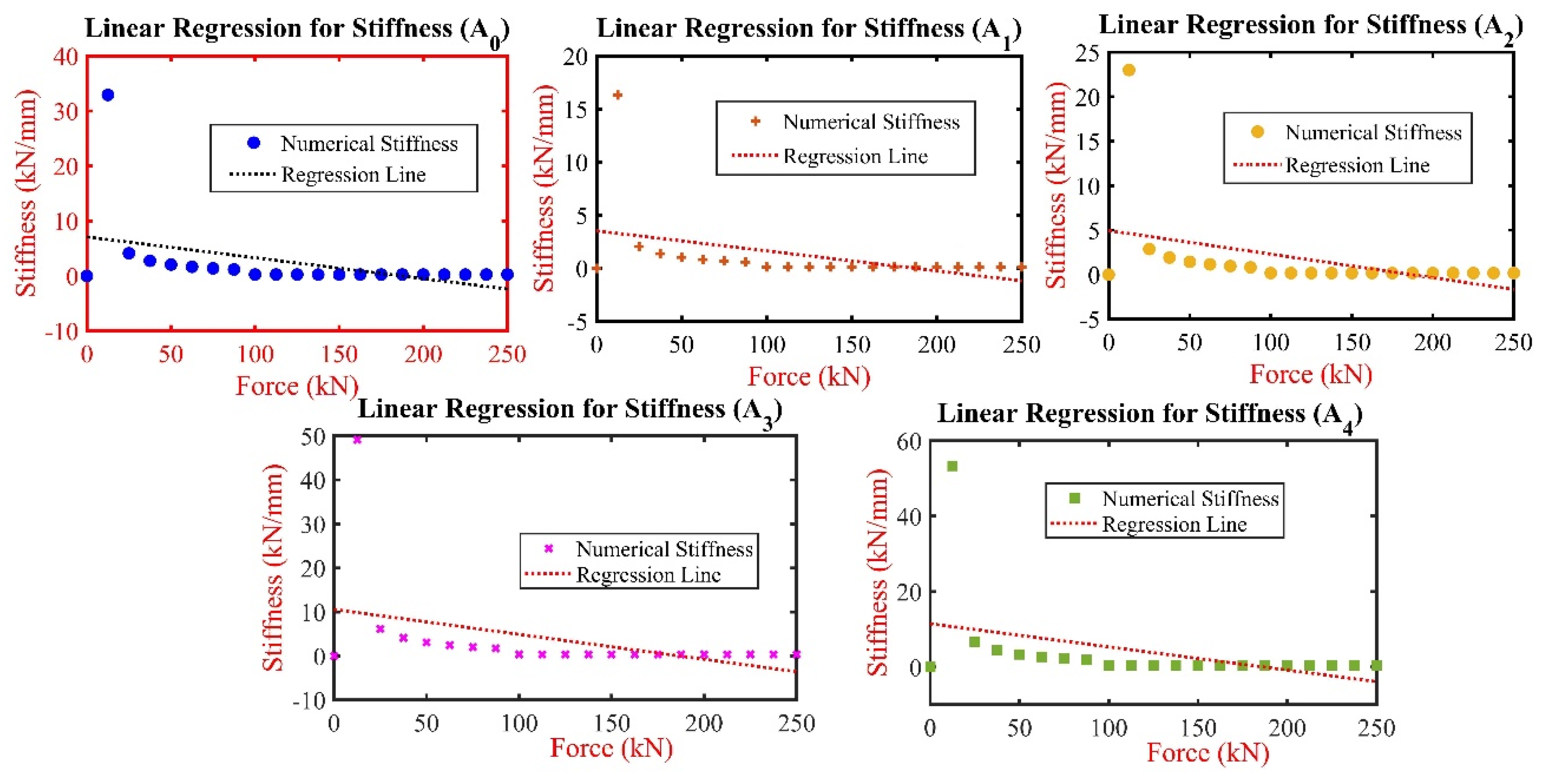
Since the previous study did not investigate the stiffness behaviour of the connection, alternative data analysis and statistics models are utilised to compare the numerical stiffness obtained using ANSYS 2023R2 with the statistical model’s data using the MATLAB R2022b algorithms approach. A linear regression analysis approach was utilised to model the relationship between force and stiffness across various attributes (stiffness A0 to stiffness A4). Aimed to understand how stiffness matrices respond to changes in applied force. The analysis commenced with defining the dataset, consisting of force value range from 0 to 250 kN at regular intervals and corresponding stiffness measurements for the five attributes (stiffness A0 through stiffness A4); linear regression was then applied to each attribute to model the stiffness as a function of force, for each stiffness attribute, the analysis process included (1) preparation of data points, associating for each force with its corresponding stiffness measurement, (2) implementation of linear regression, where the force was the independent variable and stiffness measurements acted as the dependent variable (3) visualisation of the dataset alongside the regression line, highlighting the linear relationship between force and stiffness for each attribute, and (4) calculate the R-squared value for each regression.
Figure 19 shows the linear regression analysis for stiffness attributes case (A
0 through A
4) plotted against the applied force. The analysis reveals it indicated a negative slope across all the attributes; in case (A
0), the intercept is at 7.082 kN/mm, and the stiffness decreases with increasing force, shown by a slope of -0.0379, while in case (A
1), started at an intercept of 4.5187 kN/mm, with a gentler decline in stiffness as the force increase, indicated by a slope of -0.0188; in contrast, case (A
3) be gained at a higher intercept of 10.572 kN/mm, with a more pronounced decrease in stiffness for increased force, as a slope is -0.0565. Finally, case (A
4) has the higher intercept at 11.48 kN/mm and the steepest negative slope of -0.0614, indicating the most considerable decrease in stiffness with force among the attributes. The R-squared value for all the attributes is the same (0.1724), indicating that the force explained a small portion of the variability in stiffness and that other factors might also significantly influence stiffness, such as material properties, geometry, load distribution, ageing wear, strain load, defect, etc.
5.4. Anomaly Detection Analysis
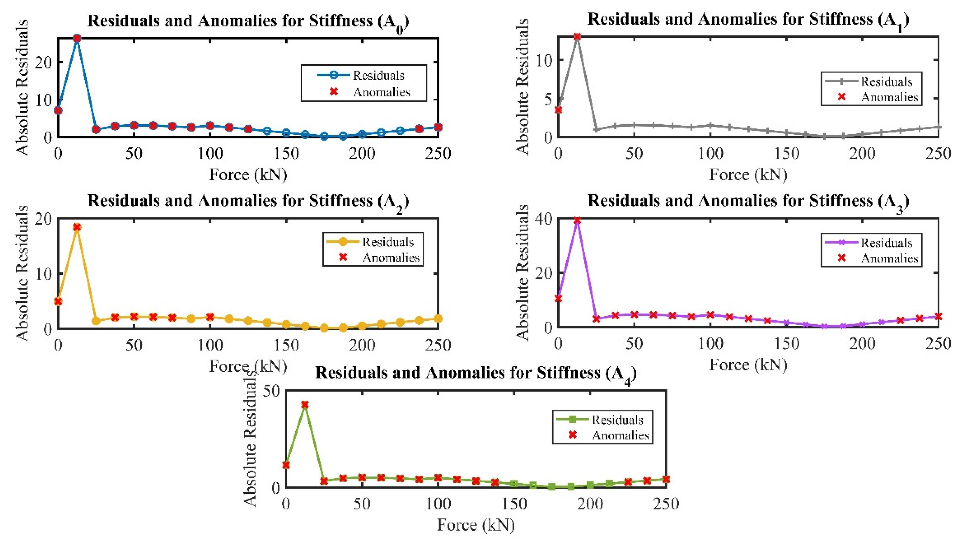
In the context of the study investigation, the anomaly detection approach focused on identifying anomalies through the analysis of residuals derived from linear regression models. This approach is pivotal for elucidating deviations from anticipated linear behaviour across a quintet of stiffness attributes (Stiffness A
0 to Stiffness A
4) against the applied force range. Employing linear regression, residuals were calculated for each attribute by deducing the difference between observed values and those predicted by the model. Subsequently, points were identified as anomalies when their absolute residuals surpassed a pre-established threshold. This procedure was instrumental in unveiling a distinct distribution of anomalies across the dataset. As shown in
Figure 20, stiffness in the controlled model (A
0) presented an extensive array of anomalies, spanning virtually the entire range of applied forces. This suggests a fundamental non-linearity in the material’s response. In contrast, case (A
1) displayed anomalies only at the onset of force application, hinting at potential setup or calibration issues. Case (A
2) showed anomalies at scattered force levels, indicating possible specific points of interest in the material’s behaviour under load. Meanwhile, case (A
3) and case(A
4) exhibited a similar pattern to (A
0), with anomalies detected across a broad spectrum of forces, underscoring a need for a deeper investigation into the structural or material properties influencing these observations. In conclusion, analysing residual and anomalies across stiffness attributes provides valuable insights into the expected and potential behaviour of the connection under investigation.
5.5. Interlocking (IMC) Plate Optimisation
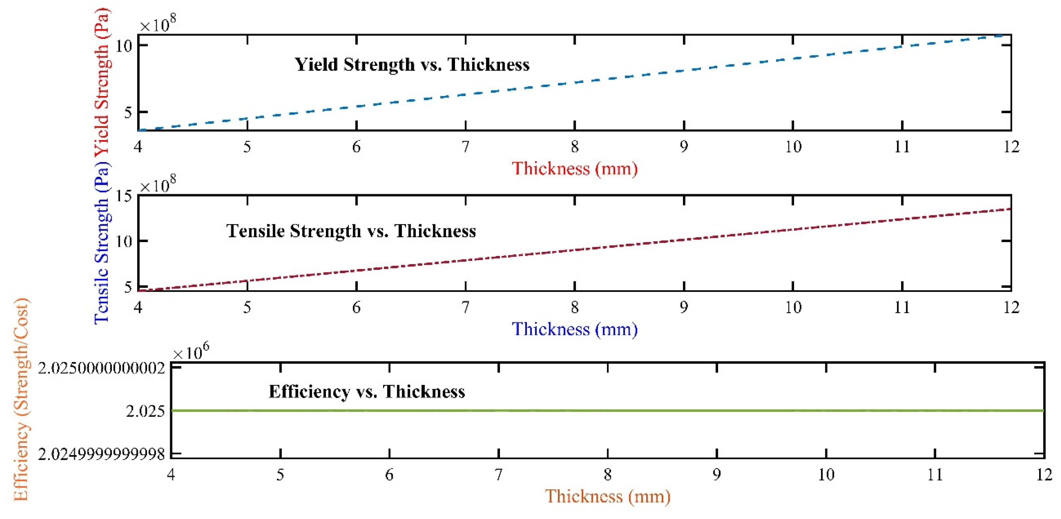
The study emphasises the crucial task of optimising the plate thickness within interlocking (IMCs) for (MSBs), levering a strategic combination of material property analysis and cost-efficiency evaluation. By employing MATLAB, the investigation systematics explores a range of plate thicknesses, from 4mm to 12mm, aiming to pinpoint the configuration that offers the optimal balance between structural integrity and economic viability. The foundation of the analysis rests on the critical material properties of G3590 steel, notably its minimum yield stress and tensile strength, alongside the cost implications tied to varying plate thickness. Through an iterative process, the study assesses the yield strength, tensile strength, and associated costs for each thickness value within the defined range, thereby deriving a composite metric of efficiency that integrates both strength characteristics and cost considerations. The analytical shown in
Figure 21 reveals notably that the yield strength and tensile strength exhibit a proportional increase with thickness, underscoring the direct relationship between structural robustness and the amount of material used. Conversely, the cost escalates linearly with increasing thickness, presenting a challenge in maintaining economic efficiency. Amidst this complex interplay of factors, the study identifies an optimal thickness that maximises the efficiency metric and creates a harmonious balance between enhancing structural properties and minimising cost. In conclusion, the optimal plate thickness, determined to be 11.03 mm, represents a reasonable choice that upholds the requisite structural integrity for MSBs while adhering to cost-effective design principles.
6. Conclusion
This paper investigates the optimum interlocking inter-module connections (IMCs) plate thickness for modular steel buildings (MSBs) using Finite Element (FE) analysis and machine learning techniques to unveil optimal configurations that balance structural integrity with economic feasibility. The major conclusions and recommendations of the investigations are presented here.
- (i)
The study identified an optimal plate thickness of 11.03 mm, underpinning a harmonious equilibrium between enhancing structural properties and ensuring economic efficiency. This thickness promises to uphold structural integrity while adhering to cost-effective design principles, showcasing a reduction in material costs by approximately 8.08% compared to thicker alternatives without compromising safety or performance standards.
- (ii)
The sensitivity analysis revealed a gradation in average sensitivity and stiffness across the attributes. The attribute Stiffness (A4) exhibited the highest average sensitivity and stiffness (0.001618 and 3.7992, respectively), suggesting a pronounced structural response to force applications by approximately 62.07% more than the controlled model (A0).
- (iii)
Employing advanced anomaly detection techniques, the study systematically highlighted inconsistencies across all attributes, significantly enhancing the predictive model’s accuracy. Advanced filtering techniques reduced noise and improved signal quality, underscoring a vital 98.5% preservation of data integrity compared to original measurements.
- (iv)
The machine learning approach, particularly the ‘TreeBagger’ random forest model, demonstrated substantial efficacy in predicting slip values based on applied force, improving prediction accuracy by up to 7% at higher force levels. This underscores the model’s robustness in handling complex, nonlinear relationships between variables.
- (v)
Through linear regression analysis, a nuanced understanding of stiffness behaviour in response to force changes was developed. This highlights the direct impact of increased plate thickness on enhancing the stability and stiffness of connections, indicating a potential increase in stiffness by up to 50.75% for thicker plates (A4) compared to thinner alternatives.
- (vi)
Evaluating the slip phenomenon across various plate thicknesses furnished valuable insights into the deformation behaviours under varying loads. The thickest plate configuration (A4) demonstrated a remarkable reduction in slip, approximately 38% lower than the controlled model (A0), illustrating the benefits of increased thickness in minimising deformation under stress.
- (vii)
Bridging Finite Element analysis with machine learning facilitated a strategic approach to plate thickness optimisation, enhancing structural performance and cost-effectiveness. The findings illuminate pathways for developing more resilient and economically viable modular steel buildings, paving the way for future advancements in construction technology and design methodologies.
This current research is limited to four interlocking (IMCs) plate sizing without consideration of environmental factors such as temperature variations, corrosion effects, and long-term wear and tear, which can significantly impact the structural integrity and performance of the connections. The study did not consider dynamic loading conditions crucial for comprehensive structural analysis and design. Future research will investigate the impact of environmental conditions on the durability and resilience of interlocking (IMCs). It will also explore the performance of these connections under dynamic loading conditions, incorporating seismic simulations and live load variations to ensure a solid understanding of their structural behaviour. Another area of interest will be developing more sophisticated predictive models that can accurately simulate the complex interactions between plate thickness, material properties, and loading conditions. Furthermore, exploring alternative materials and innovative connection designs could provide insights into optimising structural efficiency and sustainability in modular steel buildings. By addressing these gaps, future studies aim to enhance the design, safety, and versatility of interlocking inter-module connections, paving the way for their wider adoption in constructing modular steel buildings.
Author Contributions
Conceptualization, K.E. and A.A.M.; methodology, K.E. and M.E.; software, K.E., M.E. and M.R.A.; validation, M.E., A.A.M. and M.R.A.; formal analysis, K.E. and A.A.M.; investigation, K.E., M.E., and M.R.A; resources, K.E. and A.A.M; data curation, K.E. and M.E.; writing—original draft preparation, K.E. and M.E.; writing—review and editing, A.A.M. and M.R.A; visualization, K.E. and M.E; supervision, A.A.Z. and M.R.A; project administration, A.A.M., K.E., and M.E.; funding acquisition, A.A.M and K.E.
Funding
This work was financially supported by the Centre for Research and Instrumentation
Acknowledgments
The authors acknowledge the financial support from the Centre for Research and Instrumentation Management (CRIM), Universiti Kebangsaan Malaysia (UKM) [FRGS/1/2021/TK0/UKM/02/26].
Conflicts of Interest
The authors declare no conflicts of interest.
References
- Luo, F.J.; Bai, Y.; Hou, J.; Huang, Y. Progressive Collapse Analysis and Structural Robustness of Steel-Framed Modular Buildings. Eng Fail Anal 2019, 104, 643–656. [CrossRef]
- Swami, G.; Thai, T.; Thai, H.-T. Modelling Methods for Robustness Analysis of Composite Steel- Concrete Modular Buildings; ISBN 978-0-6456692-1-3.
- Farajian, M.; Sharafi, P.; Bigdeli, A.; Eslamnia, H.; Rahnamayiezekavat, P. Experimental Study on the Natural Dynamic Characteristics of Steel-Framed Modular Structures. Buildings 2022, 12. [CrossRef]
- Palmiotta, A.; Garbellini, S.; Audisio, L.; Sulla, R.; D’Amato, M.; Gigliotti, R. Seismic Behaviour of Steel Modular Buildings: Numerical Analysis and Comparisons between Different Design Solutions. In Proceedings of the Procedia Structural Integrity; Elsevier B.V., 2022; Vol. 44, pp. 1156–1163.
- Liu, X.; He, X.; Zhang, A.; Tian, C.; Zhang, X.; Tan, Y. Design and Specification Compilation of a Modular-Prefabricated High-Rise Steel Frame Structure with Diagonal Braces Part II: Elastic–Plastic Time-History Analysis and Joint Design. Structural Design of Tall and Special Buildings 2018, 27, 1–18. [CrossRef]
- Alembagheri, M.; Sharafi, P.; Hajirezaei, R.; Tao, Z. Anti-Collapse Resistance Mechanisms in Corner-Supported Modular Steel Buildings. J Constr Steel Res 2020, 170. [CrossRef]
- Chen, Z.; Zhong, X.; Liu, Y.; Liu, J. Analytical and Design Method for the Global Stability of Modular Steel Buildings. International Journal of Steel Structures 2021, 21, 1741–1758. [CrossRef]
- Yang, C.; Xu, B.; Xia, J.; Chang, H.; Chen, X.; Ma, R. Mechanical Behaviors of Inter-Module Connections and Assembled Joints in Modular Steel Buildings: A Comprehensive Review. Buildings 2023, 13, 1727. [CrossRef]
- Lee, B.; Choi, S.O. Steel Module-to-Concrete Core Connection Methods in High Rise Buildings: A Critical Review; Seoul, Korea, 2022;
- Lacey, A.W.; Chen, W.; Hao, H.; Bi, K. Review of Bolted Inter-Module Connections in Modular Steel Buildings. Journal of Building Engineering 2019, 23, 207–219. [CrossRef]
- Swami, G.; Thai, H.T.; Liu, X. Structural Robustness of Composite Modular Buildings: The Roles of CFST Columns and Inter-Module Connections. Structures 2023, 48, 1491–1504. [CrossRef]
- Chen, Z.; Khan, K.; Khan, A.; Javed, K.; Liu, J. Exploration of the Multidirectional Stability and Response of Prefabricated Volumetric Modular Steel Structures. J Constr Steel Res 2021, 184. [CrossRef]
- Chen, Z.; Wang, J.; Liu, J.; Khan, K. Seismic Behavior and Moment Transfer Capacity of an Innovative Self-Locking Inter-Module Connection for Modular Steel Building. Eng Struct 2021, 245. [CrossRef]
- Srisangeerthanan, S.; Hashemi, M.J.; Rajeev, P.; Gad, E.; Fernando, S. Review of Performance Requirements for Inter-Module Connections in Multi-Story Modular Buildings. Journal of Building Engineering 2020, 28, 101087. [CrossRef]
- Thai, H.T.; Ngo, T.; Uy, B. A Review on Modular Construction for High-Rise Buildings. Structures 2020, 28, 1265–1290. [CrossRef]
- Lacey, A.; Chen, W.; Hao, H.; Bi, K. Shear Stiffness of Bolted Inter-Module Connections. 2019.
- He, X.H.C.; Chan, T.M.; Chung, K.F. Effect of Inter-Module Connections on Progressive Collapse Behaviour of MiC Structures. J Constr Steel Res 2021, 185. [CrossRef]
- Shi, F.W.; Ding, Y.; Zong, L.; Meng, X.; Chen, Y. Axial Mechanical Behavior of Innovative Inter-Module Connection for Modular Steel Constructions. Journal of Building Engineering 2023, 65. [CrossRef]
- Lacey, A.W.; Chen, W.; Hao, H.; Bi, K. New Interlocking Inter-Module Connection for Modular Steel Buildings: Simplified Structural Behaviours. Eng Struct 2021, 227. [CrossRef]
- He, X.-H.-C.; Chan, T.-M.; Chung, K.-F. Effect of Inter-Module Connections on Progressive Collapse Behaviour of MiC Structures. J Constr Steel Res 2021, 185, 106823. [CrossRef]
- Lacey, A.W.; Chen, W.; Hao, H.; Bi, K. New Interlocking Inter-Module Connection for Modular Steel Buildings: Experimental and Numerical Studies. Eng Struct 2019, 198. [CrossRef]
- Chen, Z.; Wang, J.; Liu, J.; Cong, Z. Tensile and Shear Performance of Rotary Inter-Module Connection for Modular Steel Buildings. J Constr Steel Res 2020, 175. [CrossRef]
- Lacey, A.W.; Chen, W.; Hao, H.; Bi, K. Simplified Structural Behaviours of Post-Tensioned Inter-Module Connection for Modular Buildings. J Constr Steel Res 2020, 175. [CrossRef]
- Lacey, A.W.; Chen, W.; Hao, H.; Bi, K.; Tallowin, F.J. Shear Behaviour of Post-Tensioned Inter-Module Connection for Modular Steel Buildings. J Constr Steel Res 2019, 162. [CrossRef]
- Chen, Z.; Liu, Y.; Zhong, X.; Liu, J. Rotational Stiffness of Inter-Module Connection in Mid-Rise Modular Steel Buildings. Eng Struct 2019, 196. [CrossRef]
- Chua, Y.S.; Pang, S.D.; Liew, J.Y.R.; Dai, Z. Robustness of Inter-Module Connections and Steel Modular Buildings under Column Loss Scenarios. Journal of Building Engineering 2022, 47, 103888. [CrossRef]
- Peng, J.; Hou, C.; Shen, L. Numerical Simulation of Weld Fracture Using Cohesive Interface for Novel Inter-Module Connections. J Constr Steel Res 2020, 174, 106302. [CrossRef]
- Lacey, A.W.; Chen, W.; Hao, H.; Bi, K. Lateral Behaviour of Modular Steel Building with Simplified Models of New Inter-Module Connections. Eng Struct 2021, 236. [CrossRef]
- Shi, F.W.; Ding, Y.; Zong, L.; Chen, Y.; Wu, Y. Shear Behaviour of Vertical Inter-Module Connection with Bolts and Shear Keys for MSCs. Structures 2023, 47, 260–281. [CrossRef]
- Srisangeerthanan, S.; Hashemi, M.J.; Rajeev, P.; Gad, E.; Fernando, S. Review of Performance Requirements for Inter-Module Connections in Multi-Story Modular Buildings. Journal of Building Engineering 2020, 28. [CrossRef]
- Lateral Resistance of Multi-Story Modular Buildings Using Tenon-Connected Inter-Module Connections.
- Zhao, F.; Yu, Y.; Lin, S.; Ding, F. Evaluation of the Working Mechanisms and Simplified Models of Endplate-Type Inter-Module Connections. Structures 2021, 32, 562–577. [CrossRef]
- Zhao, F.; Yu, Y.; Lin, S.; Ding, F. Evaluation of the Working Mechanisms and Simplified Models of Endplate-Type Inter-Module Connections. Structures 2021, 32, 562–577. [CrossRef]
- Peng, J.; Hou, C.; Shen, L. Lateral Resistance of Multi-Story Modular Buildings Using Tenon-Connected Inter-Module Connections. J Constr Steel Res 2021, 177, 106453. [CrossRef]
- Lim, R.Z.C.; Looi, D.T.W.; Chen, M.T.; Tsang, H.H.; Wilson, J.L. A Component-Based Macro-Mechanical Model for Inter-Module Connections in Steel Volumetric Buildings. J Constr Steel Res 2023, 207. [CrossRef]
- Alembagheri, M.; Sharafi, P.; Hajirezaei, R.; Samali, B. Collapse Capacity of Modular Steel Buildings Subject to Module Loss Scenarios: The Role of Inter-Module Connections. Eng Struct 2020, 210. [CrossRef]
- Corfar, D.A.; Tsavdaridis, K.D. A Hybrid Inter-Module Connection for Steel Modular Building Systems with SMA and High-Damping Rubber Components. Eng Struct 2023, 289. [CrossRef]
- Lacey, A.W.; Chen, W.; Hao, H. Experimental Methods for Inter-Module Joints in Modular Building Structures – A State-of-the-Art Review. Journal of Building Engineering 2022, 46, 103792. [CrossRef]
- Farajian, M.; Sharafi, P.; Kildashti, K. The Influence of Inter-Module Connections on the Effective Length of Columns in Multi-Story Modular Steel Frames. J Constr Steel Res 2021, 177. [CrossRef]
- Dai, Z.; Pang, S.D.; Liew, J.R. Axial Load Resistance of Grouted Sleeve Connection for Modular Construction. Thin-Walled Structures 2020, 154, 106883. [CrossRef]
- He, Z.; Zhang, T.; Li, T. Static Bearing Capacity Investigation of Grouted Square Hollow Section Sleeve Connection. Advances in Structural Engineering 2022, 25, 3–13. [CrossRef]
- Dai, Z.; Cheong, T.Y.C.; Pang, S.D.; Liew, J.Y.R. Experimental Study of Grouted Sleeve Connections under Bending for Steel Modular Buildings. Eng Struct 2021, 243. [CrossRef]
- Faculty, E. Review of Interconnection in Modular Structures. 2021, 1–8.
- Lee, Y.H.; Tan, C.S.; Mohammad, S.; Md Tahir, M.; Shek, P.N. Review on Cold-Formed Steel Connections. The Scientific World Journal 2014, 2014. [CrossRef]
- Nadeem, G.; Safiee, N.A.; Bakar, N.A.; Karim, I.A.; Nasir, N.A.M. Connection Design in Modular Steel Construction: A Review. Structures 2021, 33, 3239–3256. [CrossRef]
- Pang, S.D.; Liew, J.Y.R.L.; Dai, Z.; Wang, Y. Prefabricated Prefinished Volumetric Construction Joining Tech-Niques Review. Modular and Offsite Construction (MOC) Summit Proceedings 2016, 249–256. [CrossRef]
- Rajanayagam, H.; Poologanathan, K.; Gatheeshgar, P.; Varelis, G.E.; Sherlock, P.; Nagaratnam, B.; Hackney, P. A-State-Of-The-Art Review on Modular Building Connections. Structures 2021, 34, 1903–1922. [CrossRef]
- Rajanayagam, H.; Poologanathan, K.; Gatheeshgar, P.; Varelis, G.E.; Sherlock, P.; Nagaratnam, B.; Hackney, P. A-State-Of-The-Art Review on Modular Building Connections. Structures 2021, 34, 1903–1922. [CrossRef]
- Li, Z.; Tsavdaridis, K.D.; Gardner, L. A Review of Optimised Additively Manufactured Steel Connections for Modular Building Systems. In Industrializing Additive Manufacturing; Springer International Publishing, 2021; pp. 357–373.
- Srisangeerthanan, S.; Hashemi, M.J.; Rajeev, P.; Gad, E.F.; Fernando, S. A Review of Diaphragm Behaviour and Connections for Multi-Story Modular Buildings.; 2018.
- Corfar, D.-A.; Tsavdaridis, K.D. A Comprehensive Review and Classification of Inter-Module Connections for Hot-Rolled Steel Modular Building Systems. Journal of Building Engineering 2022, 50, 104006. [CrossRef]
- Chua, Y.S.; Liew, J.Y.R.; Pang, S.D. Modelling of Connections and Lateral Behavior of High-Rise Modular Steel Buildings. J Constr Steel Res 2020, 166, 105901. [CrossRef]
- Elsayed, M.; A. Mutalib, A.; Elsayed, K. Numerical Study of Structural Performance and Wind Flow Dynamic Behavior for PPVC Steel Modular Construction (MSC) under Various Extreme Wind Loads. Buildings 2022, 12. [CrossRef]
- Sharafi, P.; Mortazavi, M.; Samali, B.; Ronagh, H. Interlocking System for Enhancing the Integrity of Multi-Storey Modular Buildings. Autom Constr 2018, 85, 263–272. [CrossRef]
- Chen, Z.; Liu, J.; Yu, Y. Experimental Study on Interior Connections in Modular Steel Buildings. Eng Struct 2017, 147, 625–638. [CrossRef]
- Chen, Z.; Liu, J.; Yu, Y.; Zhou, C.; Yan, R. Experimental Study of an Innovative Modular Steel Building Connection. J Constr Steel Res 2017, 139, 69–82. [CrossRef]
- Sanches, R.; Mercan, O.; Roberts, B. Experimental Investigations of Vertical Post-Tensioned Connection for Modular Steel Structures. Eng Struct 2018, 175, 776–789. [CrossRef]
- Chen, X.W.; Yuan, H.X.; Real, E.; Du, X.X.; Schafer, B.W. Experimental Behaviour of Stainless Steel Plate Girders under Combined Bending and Shear. J Constr Steel Res 2020, 166, 105900. [CrossRef]
- Bazarchi, E.; Davaran, A.; Lamarche, C.P.; Roy, N.; Parent, S. Experimental and Numerical Investigation of a Novel Vertically Unconstrained Steel Inter-Modular Connection. Thin-Walled Structures 2023, 183. [CrossRef]
- Ma, R.; Xia, J.; Chang, H.; Xu, B.; Zhang, L. Experimental and Numerical Investigation of Mechanical Properties on Novel Modular Connections with Superimposed Beams. Eng Struct 2021, 232. [CrossRef]
- Wu, C.; Zhou, Y.; Liu, J.; Mou, B.; Shi, J. Experimental and Finite Element Analysis of Modular Prefabricated Composite Beam-Column Interior Joints. Journal of Building Engineering 2021, 43, 102853. [CrossRef]
- Nadeem, G.; Safiee, N.A.; Bakar, N.A.; Karim, I.A.; Mohd Nasir, N.A. Experimental and Numerical Study of Self-Locking Adaptable Inter Connection for Modular Steel Structures. Journal of Building Engineering 2023, 65. [CrossRef]
- Chen, Z.; Zhong, X.; Liu, Y.; Liu, J. Analytical and Design Method for the Global Stability of Modular Steel Buildings. International Journal of Steel Structures 2021. [CrossRef]
- Deng, E.F.; Yan, J.B.; Ding, Y.; Zong, L.; Li, Z.X.; Dai, X.M. Analytical and Numerical Studies on Steel Columns with Novel Connections in Modular Construction. International Journal of Steel Structures 2017, 17, 1613–1626. [CrossRef]
- Luo, F.J.; Ding, C.; Styles, A.; Bai, Y. End Plate–Stiffener Connection for SHS Column and RHS Beam in Steel-Framed Building Modules. International Journal of Steel Structures 2019, 19, 1353–1365. [CrossRef]
- Yu, Y.; Chen, Z. Rigidity of Corrugated Plate Sidewalls and Its Effect on the Modular Structural Design. Eng Struct 2018, 175, 191–200. [CrossRef]
- Deng, E.F.; Zong, L.; Ding, Y.; Dai, X.M.; Lou, N.; Chen, Y. Monotonic and Cyclic Response of Bolted Connections with Welded Cover Plate for Modular Steel Construction. Eng Struct 2018, 167, 407–419. [CrossRef]
- Deng, E.F.; Zong, L.; Ding, Y. Numerical and Analytical Study on Initial Stiffness of Corrugated Steel Plate Shear Walls in Modular Construction. Steel and Composite Structures 2019, 32, 347–359. [CrossRef]
- Keipour, N.; Valipour, H.R.; Bradford, M.A. Structural Behaviour of Steel-Timber versus Steel-Concrete Composite Joints with Flush End Plate. Constr Build Mater 2020, 262, 120885. [CrossRef]
- Lacey, A.W.; Chen, W.; Hao, H.; Bi, K. Structural Response of Modular Buildings – An Overview. Journal of Building Engineering 2018, 16, 45–56. [CrossRef]
- Gao, Y.; Mosalam, K.M.; Chen, Y.; Wang, W.; Chen, Y. Auto-Regressive Integrated Moving-Average Machine Learning for Damage Identification of Steel Frames. Applied Sciences (Switzerland) 2021, 11. [CrossRef]
- Roy, I.G. An Optimal Savitzky–Golay Derivative Filter with Geophysical Applications: An Example of Self-potential Data. Geophys Prospect 2020, 68, 1041–1056. [CrossRef]
Figure 1.
Classification of inter-module connections (IMCs) [
51].
Figure 1.
Classification of inter-module connections (IMCs) [
51].
Figure 2.
Inter-module connection (CTC) [
21].
Figure 2.
Inter-module connection (CTC) [
21].
Figure 3.
Illustration of specimen (A) [
21].
Figure 3.
Illustration of specimen (A) [
21].
Figure 4.
Comparative thickness of plates SP14, SP15, SP16.
Figure 4.
Comparative thickness of plates SP14, SP15, SP16.
Figure 5.
Conceptual view of Lacy et al. [
21] experimental setup.
Figure 5.
Conceptual view of Lacy et al. [
21] experimental setup.
Figure 6.
Loading and boundary conditions in ANSYS 2023 R2.
Figure 6.
Loading and boundary conditions in ANSYS 2023 R2.
Figure 9.
Comparison of slip behaviour between connection plate thickness cases.
Figure 9.
Comparison of slip behaviour between connection plate thickness cases.
Figure 10.
Comparison of deformation and buckling behaviour between (A) A0, (B) A1, (C) A2, (D) A3, and (E) A4 cases.
Figure 10.
Comparison of deformation and buckling behaviour between (A) A0, (B) A1, (C) A2, (D) A3, and (E) A4 cases.
Figure 11.
Comparison of (SP14) plate and bolt deformation across (A) A0, (B) A1, (C) A2, (D) A3, and (E) A4 cases.
Figure 11.
Comparison of (SP14) plate and bolt deformation across (A) A0, (B) A1, (C) A2, (D) A3, and (E) A4 cases.
Figure 12.
Impact of plate thickness Interlocking (IMCs) stiffness behaviour.
Figure 12.
Impact of plate thickness Interlocking (IMCs) stiffness behaviour.
Figure 13.
R-squared regression coefficient.
Figure 13.
R-squared regression coefficient.
Figure 14.
Comparison of the predicted slip (∆) and Lacy et al.’s [
21] experimental results.
Figure 14.
Comparison of the predicted slip (∆) and Lacy et al.’s [
21] experimental results.
Figure 15.
Comparison between FE models (A1, A2, A3, and A4) slip and the polynomial regression predicted slips.
Figure 15.
Comparison between FE models (A1, A2, A3, and A4) slip and the polynomial regression predicted slips.
Figure 16.
Comparison between FE models (A1, A2, A3, and A4) slip and random forest prediction.
Figure 16.
Comparison between FE models (A1, A2, A3, and A4) slip and random forest prediction.
Figure 17.
Sensitivity analysis of stiffness attributes in Interlocking (IMCs) across applied forces.
Figure 17.
Sensitivity analysis of stiffness attributes in Interlocking (IMCs) across applied forces.
Figure 18.
Comparative analysis of ‘Original FE Stiffness’ and filtered data across force range.
Figure 18.
Comparative analysis of ‘Original FE Stiffness’ and filtered data across force range.
Figure 19.
Linear regression analysis of stiffness vs applied force for attributes (A0 to A4).
Figure 19.
Linear regression analysis of stiffness vs applied force for attributes (A0 to A4).
Figure 20.
Residuals and anomalies in stiffness attributes under varying forces.
Figure 20.
Residuals and anomalies in stiffness attributes under varying forces.
Figure 21.
Comparative analysis of Yield Strength, Tensile Strength, and Efficiency across plate thicknesses for IMCs in MSBs.
Figure 21.
Comparative analysis of Yield Strength, Tensile Strength, and Efficiency across plate thicknesses for IMCs in MSBs.
Table 1.
Cross-section dimensions of the module parts.
Table 1.
Cross-section dimensions of the module parts.
| Description |
Part |
Cross-Section Dimensions (mm) |
Length (mm) |
| Hollow Section |
SP10 |
75×75×6 |
50 |
| Hollow Section |
SP12 |
75×75×6 |
70 |
| Square Bar |
Bearings |
75x75 |
75 |
| Round Bar |
SP11 |
R12 |
50 |
| Plate |
SP14 |
75x8 |
75 |
| Plate |
SP15 |
75x8 |
75 |
| Plate |
SP16 |
75x8 |
135 |
| M12,8.8 |
Bolt (B) |
- |
24 |
Table 2.
Material properties.
Table 2.
Material properties.
| Part |
Grade |
Min. Yield Stress (MPa) |
Min. Tensile Strength (MPa) |
Min. Elongation (%) |
| SP10, SP12 |
C350L0 |
350 |
430 |
12 |
| Bearings |
300 |
290 |
440 |
22 |
| SP11 |
300 |
375 |
530 |
34 |
| SP14, SP15, SP16 |
G350 |
360 |
450 |
20 |
| Bolt (B) |
Class 8.8 |
640 |
800 |
12 |
Table 3.
Thickness variation of plates SP14, SP15, SP16.
Table 3.
Thickness variation of plates SP14, SP15, SP16.
| Plate |
(A0) Thickness (mm) |
(A1) Thickness (mm) |
(A2) Thickness (mm) |
(A3) Thickness (mm) |
(A4) Thickness (mm) |
| SP14 |
8 |
4 |
6 |
10 |
12 |
| SP15 |
8 |
4 |
6 |
10 |
12 |
| SP16 |
8 |
4 |
6 |
10 |
12 |
Table 4.
Range and average rate of change in stiffness.
Table 4.
Range and average rate of change in stiffness.
| Stiffness Attribute |
Min Rate of Change |
Max Rate of Change |
Average Rate of Change |
| (A0) |
-2.3034 |
2.6324 |
0.00099828 |
| (A1) |
-1.1412 |
1.3056 |
0.00049864 |
| (A2) |
-1.6108 |
1.8409 |
0.0006981 |
| (A3) |
-3.4379 |
3.929 |
0.00149 |
| (A4) |
-3.7332 |
4.2665 |
0.001618 |
|
Disclaimer/Publisher’s Note: The statements, opinions and data contained in all publications are solely those of the individual author(s) and contributor(s) and not of MDPI and/or the editor(s). MDPI and/or the editor(s) disclaim responsibility for any injury to people or property resulting from any ideas, methods, instructions or products referred to in the content. |
© 2024 by the authors. Licensee MDPI, Basel, Switzerland. This article is an open access article distributed under the terms and conditions of the Creative Commons Attribution (CC BY) license (http://creativecommons.org/licenses/by/4.0/).
