High-precision Quality Prediction Based on Two-dimensional Extended Windows

Preprint

Article

High-precision Quality Prediction Based on Two-dimensional Extended Windows

Altmetrics

Downloads

Views

Comments

A peer-reviewed article of this preprint also exists.

This version is not peer-reviewed

Submitted:

29 March 2024

Posted:

29 March 2024

You are already at the latest version

Alerts

Abstract

A PLS-based quality prediction method is proposed for batch processes using two-dimensional extended windows. To realize the adoption of information in the direction of sampling time and batch, a new definition region of support (ROS), k-i-back-extended region of support (KIBROS), is proposed to establish the extended window, which including the data of the previous sampling times in the same batch, the data of the same sampling time in the historical batches, the data of the previous sampling times in the historical batches and the data of the later sampling times in the historical batches. According to these regions of support, extended windows are established, and different models are proposed based on the extended windows for batch processes quality prediction. Further, using a typical batch process as an example, the injection molding process, the proposed quality prediction method is experimentally verified, proving that the proposed methods have higher prediction accuracy than the traditional method and the prediction stability is also improved.

Keywords:

Subject: Engineering - Control and Systems Engineering

1. Introduction

Precise variable prediction modeling depends on a good understanding of process characteristics. Industrial processes usually have characteristic changes along two directions. The first is the time direction within a production period where main conditions do not change but some will shift due to complex factors. Usually, during the production period, only one kind of production is provided. The characteristic changes along this direction lead to a series of phases. The second is the repeat production direction where main conditions can be kept to obtain the same products but the time-varying problem may still happen or main conditions can be changed systematically to obtain different productions.

Multivariate statistical modeling methods are typical data-driven modeling methods, among which principal component analysis (PCA) [1] and partial least squares (PLS) [2] have been applied widely in the fields of industrial process modeling, monitoring, and control [3,4,5]. Especially, for batch processes, multilinear principal component analysis (MPCA) and multiway partial least squares regression (MPLS) are classic methods dealing with the three-dimensional matrix by enfolding it into a two-dimensional matrix [6,7]. Following their work, a lot of research works have been proposed [8,9,10,11,12]. Among them, a certain number of papers focused on the multi-phase characteristic where different statistical models are built for different phases [11,12] and the relationship between phases is investigated for better modeling and prediction [13]. For both continuous processes and batch processes, the sliding window method is very typical to deal with the time-varying problem [12], and multiple models are usually built for multiple modes [14,15,16,17]. As can be seen above, the characteristic changes along the time direction and the repeat production direction have been quite interesting for researches. However, these research works tend to deal with one problem in each work, that is, they tend to deal with the characteristic change problem only in one direction. This makes it difficult to apply these methods because usually the characteristic may change in the two directions simultaneously. Thus, it is necessary to investigate a uniform modeling method which can deal with characteristic changes in the two directions simultaneously.

Recently, a complete set of process modeling method has been developed to solve the process characteristic evolution problem in both the intra-batch and inter-batch directions [18], where the problems in two directions are firstly handled separately, and then the two strategies are combined. This kind of approach is flexible to select appropriate modeling methods in two directions [19]. However, the separation of methods is unavoidable. It is hard to give a comprehensive explanation of the process characteristics under the two irrelevant methods. In addition, when the methods in both directions need to be jointed, the method structure is relatively complex and difficult to comprehend and implement. Afterwards, a two-dimensional, two-layer quality regression model is established to monitor multi-phase, multi-mode batch processes [20]. In this method, the two-dimensional regression traces the intra-batch and inter-batch characteristics, while the two-layer structure establishes the relationship between the target process and historical modes and phases. However, the two-layer structure is more suitable for the multi-mode characteristic and the multi-phase characteristic, but not suitable for the slow time-varying characteristics in the two directions. Therefore, it is necessary to develop a set of modeling strategies tracing the slow time-varying intra-batch and inter-batch characteristics simultaneously.

In this paper, aiming at the industrial processes with the slow time-varying characteristic along both the time direction and the repeat production direction, a modeling algorithm using two-dimensional extended windows is proposed for quality prediction. The data of previous batches and previous sampling times are both considered to be correlated with the current sampling data, which can bring more precision in the online prediction of product quality. Therefore, an improved ROS, KIBROS, will be defined, which including the data of the previous sampling times in the same batch (KROS), the data of the same sampling time in the historical batches (IROS), the data of the previous sampling times in the historical batches (KIROS) and the data of the later sampling times in the historical batches (BROS). Based on that, the i-extended window, k-extended window, i-k-extended window, back-extended window, and i-k-back-extended window will be proposed. Finally, quality prediction models will be constructed using the extended windows. The injection molding process will be used as the example for experimental verification. Finally, suggestions are given for the usage of the extended windows based quality prediction methods.

The remaining work of this paper includes the following aspects: in the second section, the quality prediction algorithm, partial least squares (PLS), and the establishment of sliding window is introduced first, then the modeling strategy with the extended ROS, especially two-dimensional i-k-back-extended ROS is proposed, followed by the quality prediction method and two evaluation indicators. The application of the proposed method to the injection modeling process is introduced in the third section. The fourth section is the conclusion.

2. Methodology

2.1. Partial Least Squares Method (PLS)

For a typical batch process, the process data is often stored in the form of a three-dimensional matrix, which is denoted as

\bar{X} (I \times J_{x} \times K)

, where I represents the number of batches,

J_{x}

represents the number of process variables, and

K

represents the number of sampling points in a batch. Meanwhile, at the end of one batch operation, the quality data can be obtained, which is stored in the form of a two-dimensional matrix, denoted as

Y (I \times J_{y})

, where

J_{y}

represents the number of quality variables. PLS is a classical regression method for quality prediction industrial processes. It can not only carry out regression modeling, but also simplify the structure of data, and analyze the correlation between two groups of variables [16,21]. Using the PLS algorithm, the correlation between process variables and quality variables can be transformed into the latent variable space for research. It should be pointed out that the inputs of PLS should be two-dimensional matrices. Therefore, before using PLS for modeling, it is necessary to expand the process data matrix into time slices or other two-dimensional matrices [22]. Its main formula is as follows:

\begin{array}{l} X = T P^{T} + E = \sum_{a = 1}^{A} t_{a} p_{a}^{T} + E \\ Y = U Q^{T} + F = \sum_{a = 1}^{A} u_{a} q_{a}^{T} + F \end{array}

(1)

where T and U represent the score matrices, P and Q represent the load matrices, and E and F represent the residual matrices.

The regression model based on PLS is as follows:

Y = X B

(2)

where B is the regression coefficient matrix.

2.2. Establishment of Sliding Window

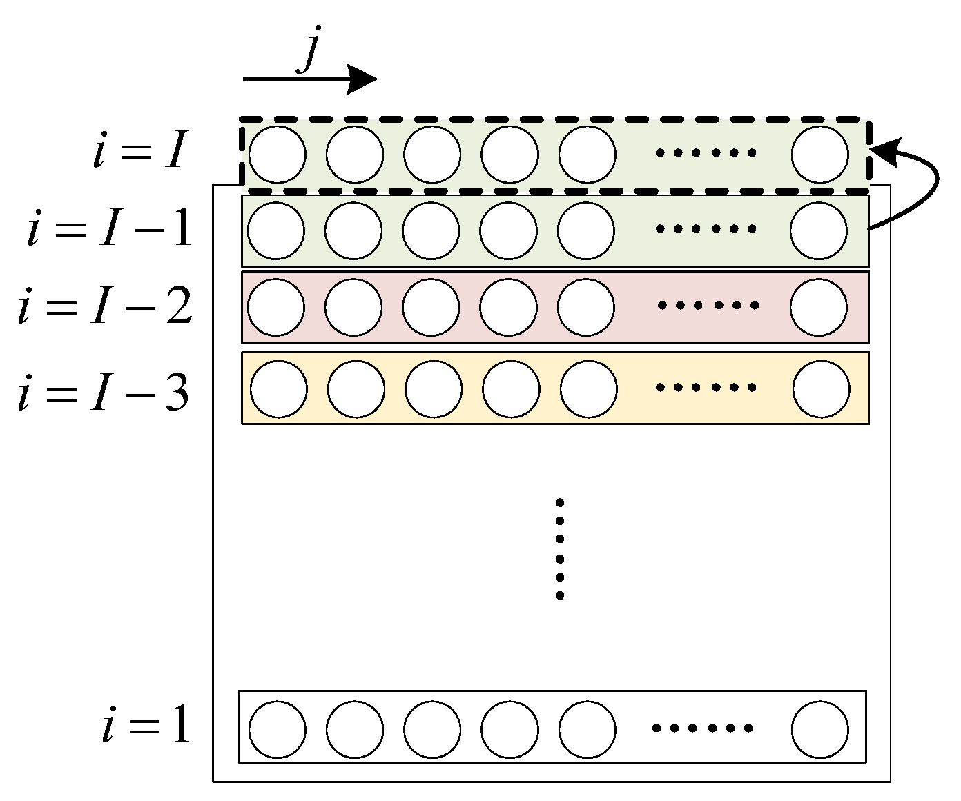
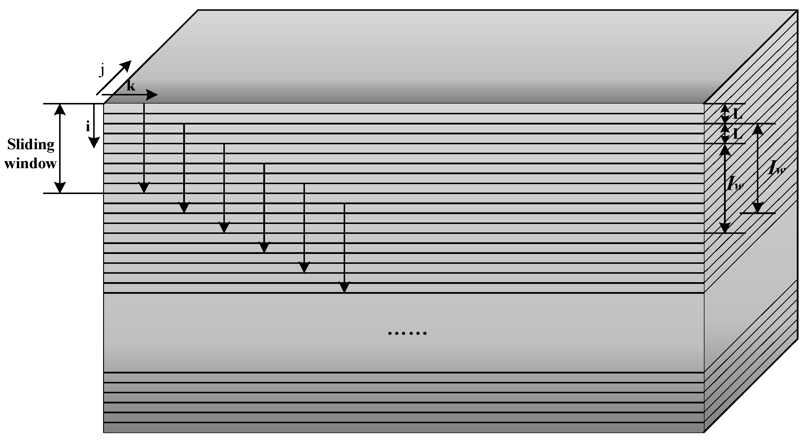
Usually, a batch process needs to be divided into several phases using some production knowledge of the specific process, and critical-to-quality phases and critical-to-quality variables should be identified. These phases will then be treated separately. Within phases, the slow time-varying problem is characterized by the relationship change between process variables and quality variables from batch to batch. The key step of analysis is to divide the slow-time-varying batch process into different modes and build different models according to different modes. The sliding window method is adopted in this paper, and its demonstration diagram is shown in Figure 1. In this figure, i represents the batch direction, j represents the process variable direction, and k represents the direction of the sampling points in a batch. The first window is established using the process data of the first

I_{w}

batch, where the process variable matrix is denoted as

X (I_{w} \times J_{x} \times K)

and the corresponding quality data is denoted as

Y (I_{w} \times J_{y})

. When sliding, the window is moved down by L batches each time, that is, the second window is formed by using the data of

(L + 1)

-th to

(L + I_{w})

-th batches. L is advised to be 1 [23].

The process data

X

in sliding window can be divided into K time slices, the k-th can be represented as

X_{k} (I_{w} \times J_{x})

, and traditionally, PLS model can be built between the time-slice data

X_{k}

and the quality data

Y

. Next in the work, each element in the time-slice data

X_{k}

x_{i, k} (1 \times J_{x})

, will be extended by novel ROSs.

2.3. Two-Dimensional Extended ROS

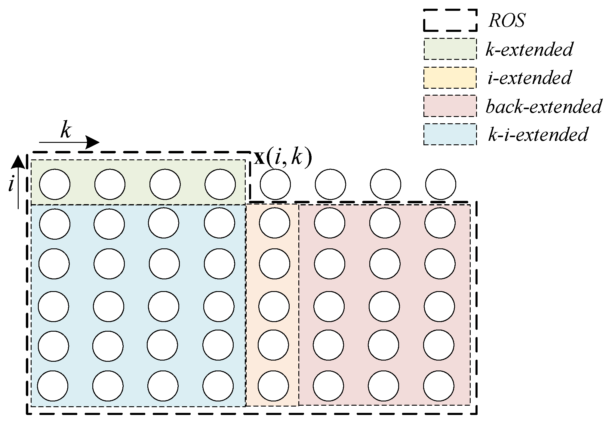
The schematic diagram of the ROS proposed in this paper is shown in Figure 2. For convenience, for the process data,

X (I_{w} \times J_{x} \times K)

, the variable direction is not shown in the figure and each circle represent a sample point

x_{i, k} (1 \times J_{x})

. The previous neighbors of

x_{i, k}

, which may have an impact on it, including not only the past points in the time direction,

x_{i, k - 1}

x_{i, k - 2}

,…,

x_{i, 1}

, but also the past points in the batch direction,

x_{i - 1, k}

x_{i - 2, k}

,…,

x_{1, k}

, the past points in both the time direction and the batch direction,

x_{i - 1, k - 1}

x_{i - 1, k - 2}

,…,

x_{i - 1, 1}

x_{i - 2, k - 1}

,…,

x_{i - 2, 1}

,…,

x_{1, 1}

, and even the past points of the past batches but with the time indexes larger than k,

x_{i - 1, k + 1}

x_{i - 1, k + 2}

,…,

x_{i - 1, K}

x_{i - 2, k + 1}

,…,

x_{i - 2, K}

,…,

x_{1, k + 1}

,…,

x_{1, K}

. The region covering the above points which may influence the contribution of the current point to the final quality is defined as the novel ROS. Thus, these four parts of data are called the k-extended region of support (KROS), i-extended region of support (IROS), k-i-extended region of support (KIROS) and back-extended region of support (BROS). Their specific locations are shown in Figure 2. The novel ROS, k-i-back-extended region of support (KIBROS), include the above four ROSs.

In the cited paper [24], the ROS was defined as the data before the time point of this batch and previous batches, which including k-extended and k-i-extended ROSs in Figure 2. While, in this paper, ROS is redefined and extended to four sub-regions including all possible regions along the time direction and the batch direction. Correspondingly, the observed element

x_{i, k}

will be extended in the four specific ROSs.

In the previous batch process research, the variable data of the k-th sampling time in each batch are formed into a time-slice matrix,

X_{k} (I \times J_{x})

, and used to find the relationship between the sampling process data and the quality data, and then all time-slice matrices are used to obtain the final prediction quality [25]. In this work, all samples in ROSs are considered at the same time while modeling for each sampling point, thus the established model will contain the corresponding information, and the prediction accuracy can be further improved. Based on the above data in ROSs, a two-dimensional extended matrix is proposed, whose specific description is as follows.

Step 1. Extension of samples in the k-extended region of support (KROS).

The past points in the time direction, that is, the samples in KROS,

x_{i, k - 1}

x_{i, k - 2}

,…,

x_{i, 1}

, are considered to construct the extended ROS in the time direction. And the extended process data matrix can be obtained as below, while the quality data vector remains since it represents the final quality for the whole batch. It should be noticed that for the final quality which can only be obtained at the end of each batch process, the k index is not necessary.

x_{i, k}^{F} = [x_{i, k - F + 1}, \dots, x_{i, k - 1}, x_{i, k}]

(3)

y_{i}^{F} = y_{i}

(4)

where

F

represents the total number of sampling times included, in other words, a total

F - 1

of sampling times are extended forward.

Step 2. Extension of samples in the i-extended region of support (IROS).

Next is the way to build the extended ROS in the batch direction. For the variable vector of the i-th batch at the k-th sampling time,

x_{i, k} (1 \times J)

, the variable vector of the (i-1)-th batch,

x_{i - 1, k}

is spliced at the back of

x_{i, k}

, and the variable vector of (i-2)-th, (i-3)-th, ..., (i-N+1)-th batch are spliced behind the matrix in turn, where N is the number of batches included. The extended process variable matrix is shown below, and similarly, the quality matrix is established.

X_{i, k}^{N} = [\begin{array}{l} x_{i, k} \\ x_{i - 1, k} \\ ⋮ \\ x_{i - N + 1, k} \end{array}]

(5)

Y_{i}^{N} = [\begin{array}{l} y_{i} \\ y_{i - 1} \\ ⋮ \\ y_{i - N + 1} \end{array}]

(6)

Step 3. Extension of samples in the k-i-extended region of support (KIROS).

Combining the KROS and the IROS proposed before, the method proposed next can further realize the construction of a two-dimensional extended matrix based on the time-batch evolution information.

First, for the i-th batch, the data are extended in the direction of sampling time according to the method mentioned in Step 1 to obtain a matrix

x_{i, k}^{F}

Then, the i-th to the (i-N+1)-th batches in the IROS are extended according to the time direction, and the following process data extended matrix is obtained, as well as the quality data extended matrix:

X_{i, k}^{F, N} = [\begin{matrix} x_{i, k - F + 1} & \dots & x_{i, k - 1} & x_{i, k} \\ x_{i - 1, k - F + 1} & \dots & x_{i - 1, k - 1} & x_{i - 1, k} \\ ⋮ & ⋱ & ⋮ & ⋮ \\ x_{i - N + 1, k - F + 1} & \dots & x_{i - N + 1, k - 1} & x_{i - N + 1, k} \end{matrix}]

(7)

Y_{i}^{F, N} = [\begin{array}{l} y_{i} \\ y_{i - 1} \\ ⋮ \\ y_{i - N + 1} \end{array}]

(8)

Step 4. Extension of samples in the back-extended region of support (BROS).

Since in the above work, only the data before the k-th sample time is adopted, it is necessary to further consider the data information after the k-th sample time to further improve the accuracy of quality prediction. The construction method of the backward extended matrix is symmetric with the two-dimensional extended matrix based on the time-batch evolution information proposed in the previous step. In addition, since the information of the current i-th batch after the k-th sample time is unable to be obtained during modeling, considering the similarity of processes between batches in the batch process, the data after the k-th time of the (i-1)-th batch is used as an alternative, then the corresponding position of the current batch is filled. A schematic diagram of the specific process is shown in Figure 3.

A backward extended process data matrix and a backward extended quality matrix can be constructed using the above-mentioned method in the direction of batch and sampling time as below:

X_{i, k}^{B} = [\begin{matrix} x_{i - 1, k + 1} & x_{i - 1, k + 2} & \dots & x_{i - 1, k + B} \\ \begin{array}{l} x_{i - 1, k + 1} \\ x_{i - 2, k + 1} \end{array} & \begin{array}{l} x_{i - 1, k + 2} \\ x_{i - 2, k + 2} \end{array} & \begin{array}{l} \dots \\ \dots \end{array} & \begin{array}{l} x_{i - 1, k + B} \\ x_{i - 2, k + B} \end{array} \\ ⋮ & ⋮ & ⋱ & ⋮ \\ x_{i - N + 1, k + 1} & x_{i - N + 1, k + 2} & \dots & x_{i - N + 1, k + B} \end{matrix}]

(9)

Y_{i}^{B} = [\begin{array}{l} y_{i} \\ y_{i - 1} \\ y_{i - 2} \\ ⋮ \\ y_{i - N + 1} \end{array}]

(10)

where B is the number of backward samples included.

Step 5. Extension of samples in the k-i-back-extended region of support (KIBROS).

The sampled data in the whole range of ROS are used, and a method for constructing a k-i-back-extended matrix based on time-batch evolution information is proposed next. For the process data at the k-th sampling time in the i-th batch currently considered,

x_{i, k}

, first, it is extended in the direction of the sampling time to obtain

X_{i, k}^{F, N, B}

, which is expressed as follows, as well as the quality data:

X_{i, k}^{F, N, B} = [\begin{matrix} x_{i, k - F + 1} & \dots & x_{i, k - 1} & x_{i, k} \\ x_{i - 1, k - F + 1} & \dots & x_{i - 1, k - 1} & x_{i - 1, k} \\ ⋮ & ⋱ & ⋮ & ⋮ \\ x_{i - N + 1, k - F + 1} & \dots & x_{i - N + 1, k - 1} & x_{i - N + 1, k} \end{matrix} \begin{matrix} x_{i - 1, k + 1} & x_{i - 1, k + 2} & \dots & x_{i - 1, k + B} \\ x_{i - 1, k + 1} & x_{i - 1, k + 2} & \dots & x_{i - 1, k + B} \\ ⋮ & ⋮ & ⋱ & ⋮ \\ x_{i - N + 1, k + 1} & x_{i - N + 1, k + 2} & \dots & x_{i - N + 1, k + B} \end{matrix}]

(11)

Y_{i}^{F, N, B} = [\begin{array}{l} y_{i} \\ y_{i - 1} \\ ⋮ \\ y_{i - N + 1} \end{array}]

(12)

The parameters that determine the size of the expanded matrix are F, N and B as mentioned before. In actual construction, three parameters can be determined one by one to achieve the best prediction effect.

As introduced before, the quality prediction model will be built between the time-slice data

X_{k}

and the quality data

Y

. In this work, each element in the time-slice data

X_{k}

x_{i, k} (1 \times J_{x})

, will be extended by the proposed

x_{i, k}^{F}

X_{i, k}^{N}

X_{i, k}^{F, N}

X_{i, k}^{B}

, and

X_{i, k}^{F, N, B}

, according to the proposed new ROSs, obtaining the extended time-slice data

X_{k, e x}

. Similarly, each element in the quality data

Y

y_{i}

, will be extended by the proposed

y_{i}^{F}

Y_{i}^{N}

Y_{i}^{F, N}

Y_{i}^{B}

, and

Y_{i}^{F, N, B}

, obtaining the extended quality data

Y_{e x}

. Subsequently, the quality perdition model will be built.

2.4. Quality Prediction Method and Evaluation Indicators

After the construction of the extended data matrix within each sliding window is given, PLS is used to finish the quality prediction. As mentioned before, the PLS model based on the extended window is expressed as follows:

\begin{array}{l} X_{c, k, e x} = T_{c, k, e x} P_{c, k, e x}^{T} + E_{c, k, e x} = \sum_{a = 1}^{A} t_{c, k, e x, a} p_{c, k, e x, a}^{T} + E_{c, k, e x} \\ Y_{c, e x} = U_{c, k, e x} Q_{c, k, e x}^{T} + F_{c, k, e x} = \sum_{a = 1}^{A} u_{c, k, e x, a} q_{c, k, e x, a}^{T} + F_{c, k, e x} \end{array}

(13)

where

X_{c, k, e x}

represents the extended time-slice data matrices,

Y_{c, e x}

represents the extended quality data matrices, where c represent the c-th phase for multi-phase processes. The regression model is as follows:

Y_{c, e x} = X_{c, k, e x} B_{c, k, e x}

(14)

For the batch whose quality to be predicted online, the process variable matrix is denoted as

X_{k}^{*}

. The extended matrix of this test batch is established using the method proposed in Section 2.3, donated as

X_{c, k, e x}^{*}

, and it is substituted into the following formula to obtain the prediction quality.

{\tilde{Y}}_{c, k, e x} = X_{c, k, e x}^{*} B_{c, k, e x}

(15)

A few indicators are used to evaluate the performance of prediction methods based on the model. The prediction accuracy,

R_{k, c}^{2}

, of the quality prediction model of the k-th sampling time within the c-th phase is as follows:

R_{k, c}^{2} = \frac{\sum_{i = 1}^{I} {({\tilde{y}}_{i, c, k, e x} - \bar{y})}^{2}}{\sum_{i = 1}^{I} {(y_{i} - \bar{y})}^{2}}

(16)

where

y_{i}

is the measured value of the quality variable of the i-th batch,

{\tilde{y}}_{i, c, k, e x}

is the predicted value of the one of quality variables of the k-th sampling time within the c-th phase and

\bar{y}

is the average value of the quality variable measured at the end of the i-th batch. The value range of

R_{k, c}^{2}

is 0-1. If

R_{k, c}^{2}

approaches 1, it indicates that the precision of the quality prediction model is high. While if

R_{k, c}^{2}

approaches 0, it means that the change in this phase cannot explain the change of quality well.

Furthermore,

\bar{R_{c}^{2}}

is proposed to indicate the average impact of the c-th phase:

\bar{R_{c}^{2}} = \sum_{k = k_{s t a r t}}^{k_{e n d}} R_{k, c}^{2} / (k_{e n d} - k_{s t a r t})

(17)

where

k_{s t a r t}

and

k_{e n d}

represent the starting and last sampling points in the c-th phase, separately. In this paper, the offline quality analysis will be carried out based on the comparison of

\bar{R_{c}^{2}}

and

R_{k, c}^{2}

Root mean square error (RMSE) is used to verify the prediction accuracy of the model, which is expressed by the following formula:

RMSE = \sqrt{\sum_{i = 1}^{r} d_{i}^{2} / r}

(18)

where r is the number of measurement groups and

d_{i}

is the deviation between one group of the predicted values and the real value of quality. As can be seen from the formula, the smaller the RMSE, the more accurate the prediction results. The comparison of the online prediction precision of each method is based on the evaluation of RMSE.

3. Illustration and Discussions

This section may be divided by subheadings. It should provide a concise and precise description of the experimental results, their interpretation, as well as the experimental conclusions that can be drawn.

3.1. Introduction of Injection Molding Process

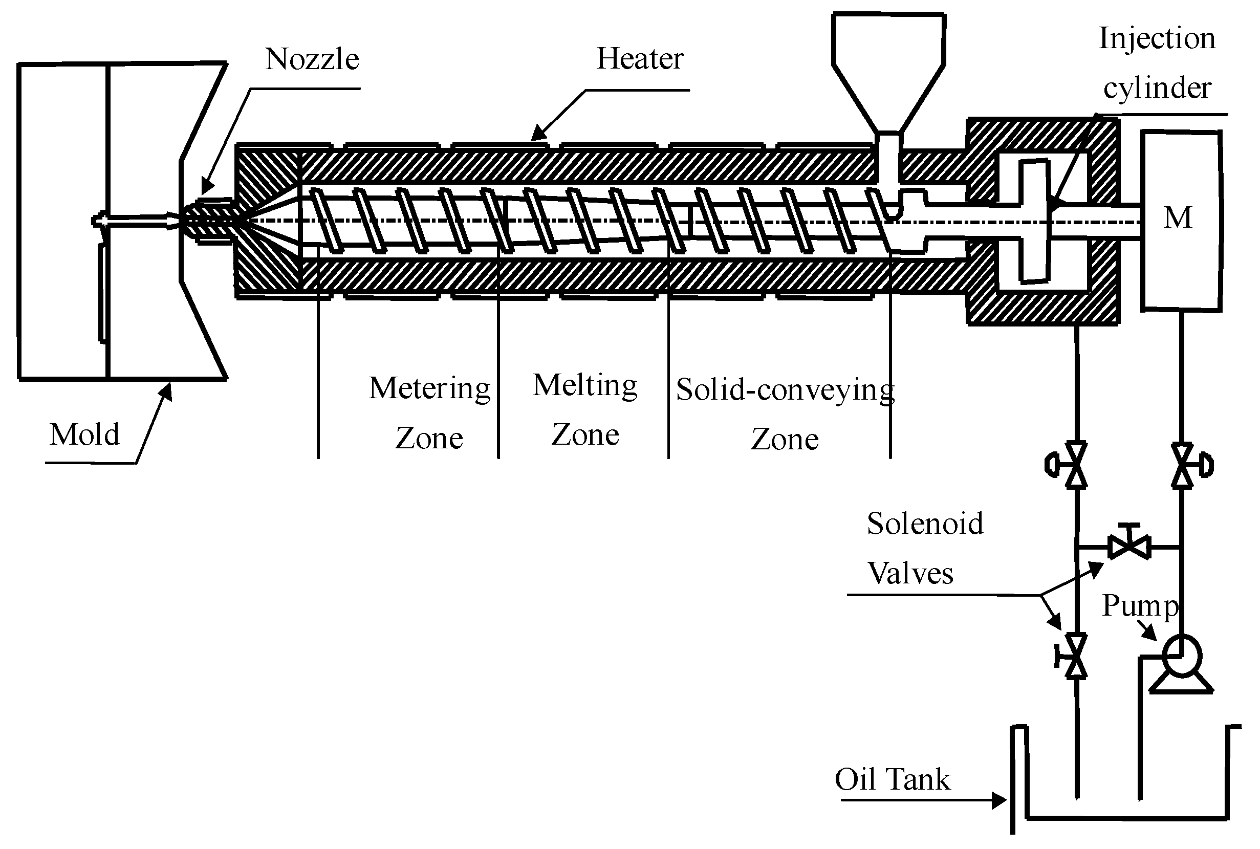
Injection molding technology is an important plastic processing method, and the injection molding process is a typical batch process. During the injection molding process, there are often drifts in operating conditions and other unknown perturbations that can lead to unstable product quality. Therefore, how to accurately predict the product quality to adjust the process parameters in time so that the product quality can meet the requirements again is the basic research direction of the quality control of the injection molding process. A schematic diagram of a typical injection molding machine is shown in Figure 4.

According to the characteristics of injection molding processes, the entire injection molding process is divided into four phases, namely injection phase, pressure holding phase, plasticization phase and cooling phase. These four phases are considered to be the critical-to-quality operation phases that determine product quality. During the injection molding process, many process variables will affect the final product quality, and the values of these process variables can be measured by corresponding sensors; at the end of each batch, the product quality information, that is the weight of each product, can also be measured. The key process variables involved in this experiment are listed in Table 1.

3.2. Variable Analysis of Injection Molding Process and Experiment Condition

The material used in this work is high density polyethylene (HDPE), and the specific operating conditions are shown in Table 2. In the experiment, the sampling information of 100 batches of the real injection molding process is selected. Each batch contains 919 sampling points.

Based on the knowledge of the injection molding process, all sampling points in a batch are divided into four phases. The sample points of the injection phase are samples 1-220; the sample points of the packing-holding phase are samples 221-519; the sample points of the plasticizing phase are samples 520-729; the sample points of the cooling phase are samples 730-919.

The method mentioned in Section 2.2 is used to establish sliding windows. The number of batches in each window is 30, the sliding step size is L=1, and a total of 71 sliding windows are established.

3.3. Application of Prediction Model and Identification of Related Parameters

3.3.1. Application of One-Dimensional Extended Window Model Using the Samples in KROS Only

Prediction model using k-extended data matrices in KROS based on sampling time information is constructed within each sliding window using the method mentioned in Section 2. The number of sampling times for forward extension, F, changes from 0 to 10, and for the c-th phase, the indicator

\bar{R_{c}^{2}}

values are analyzed to judge the predictive ability of the model, which are given in Table 3.

It can be seen that in different phases, the changing trend of

\bar{R_{c}^{2}}

is roughly rising, and at the same time, this rising trend is gradually slowing down. Therefore, to balance the prediction accuracy and the algorithm complexity, it is necessary to set a threshold

ε

, and stop the extension when the rate of change is less than this threshold. The expression for the change rate can be written as:

Δ = \frac{|\bar{R_{c, F + 1}^{2}} - \bar{R_{c, F}^{2}}|}{\bar{R_{c, F}^{2}}}

(19)

where

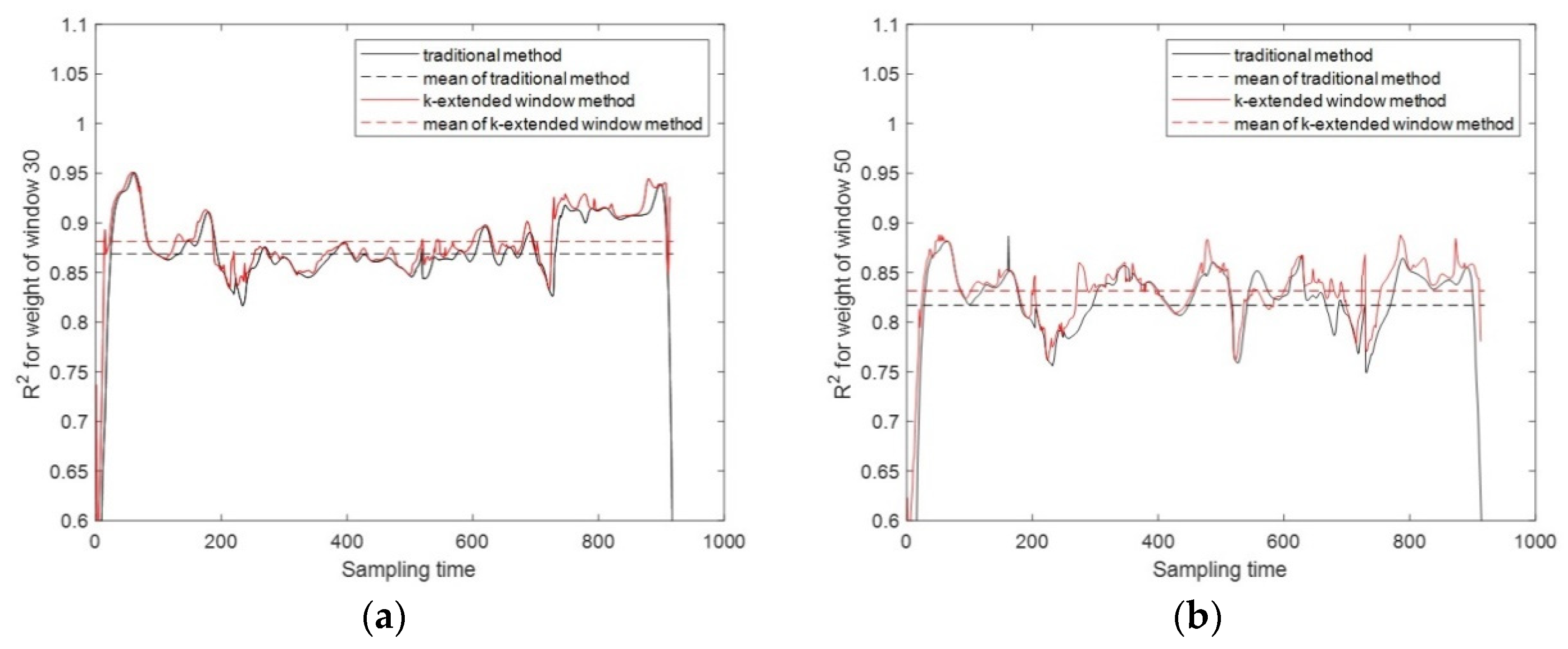
\bar{R_{c, f}^{2}}

represents the value of

\bar{R_{c}^{2}}

in the situation that the extended window includes F-1 forward sampling time for modeling. If

ε

is taken as 0.0025, then F=6. Therefore, in the following discussion, F is assigned a value of 6. Taking sliding window 30 and sliding window 50 as examples,

R_{k, c}^{2}

of each sampling time and the mean value of the whole sampling times is given in Figure 5.

Figure 5 shows the performance of the quality prediction model constructed by the traditional method and the method based on the k-extended window method. As can be seen from Figure 5, using the extended window modeling in the sampling time direction, from the perspective of sampling times, the average performance is boosted, and most

R_{k, c}^{2}

of the sampling points have been improved. The discussion above verifies the rationality of the proposed method based on the k-extended window method.

3.3.2. Application of Extended Window Model Using the Samples in IROS and KIROS

Similarly, the prediction model using i-extended data matrices in IROS based on batch information is constructed within each sliding window using the method mentioned in Section 2, as well as the prediction model using the k-i-extended data matrices in KIROS. The number of sampling times for forward extension, F, is uniformly set to 0 and 6, and on this basis, the number of extended batches, N, changes from 0 to 10. The indicator

\bar{R_{c}^{2}}

values are analyzed to judge the predictive ability of the model, which are given in Table 4.

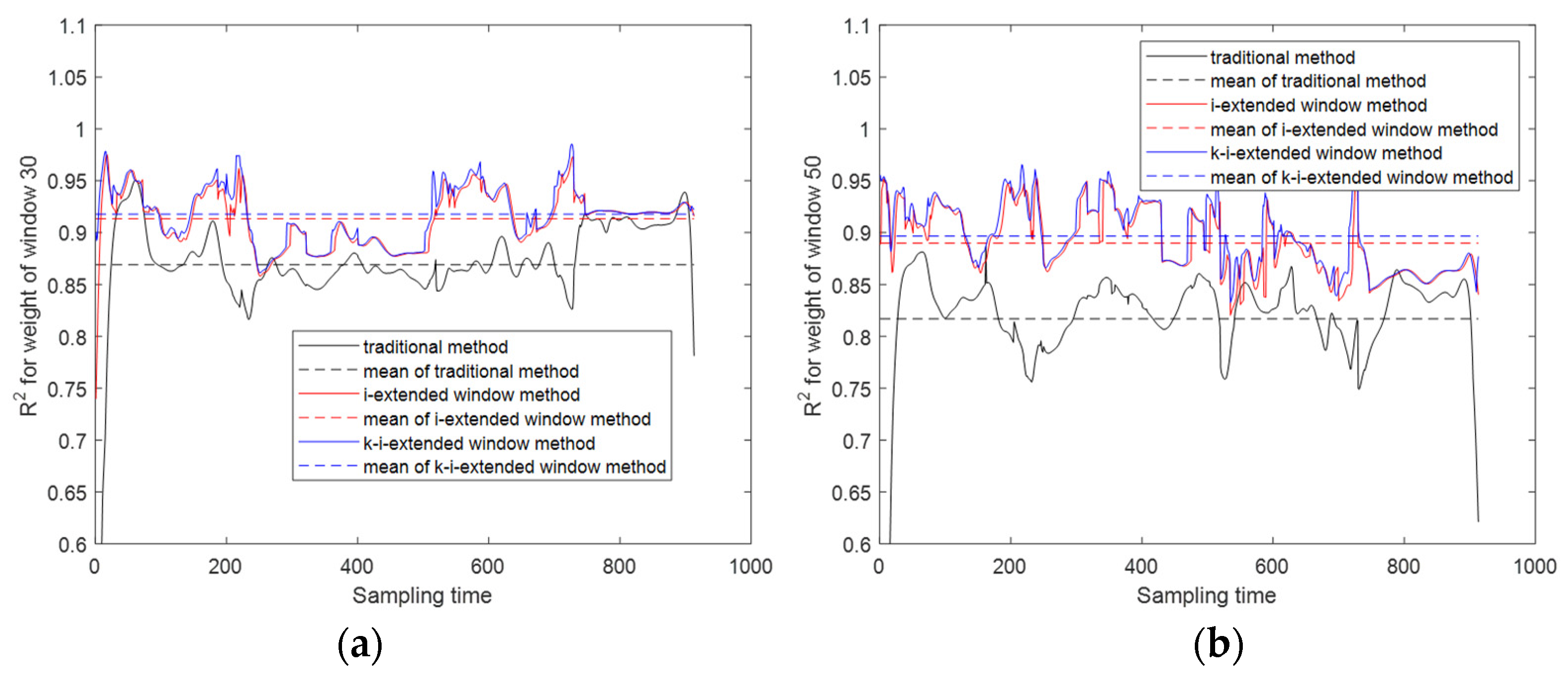
It can be easily found from the table that

\bar{R_{c}^{2}}

are roughly rising, and at the same time, the rising rates are gradually decreasing. Here the threshold,

ε

, is 0.015, then N is set to 5. From the above table, the following conclusions can be drawn. First, when 10 batches are extended downward, the

\bar{R_{c}^{2}}

values of Phase 1, Phase 2 and Phase 4 all reach more than 0.9. Compared with the extended window in the sampling time direction, the extended window in the batch direction can achieve a better prediction effect; Second, comparing the cases where F is 0 and F is 6 in the table, it can be found that the

\bar{R_{c}^{2}}

of the latter is higher than the former under the condition of the same batch extension quantity. That is, when the windows both in the direction of sampling time and batch are used in combination, the effect is superimposed. This illustrates the rationality of constructing a two-dimensional extended window based on time-batch evolution information. Window 30 and window 50 are also selected to give the

R_{k, c}^{2}

values of each sampling time, as shown in Figure 6.

Figure 6 shows the performance of the quality prediction model constructed by three methods: the traditional method, the method based on the i-extended window, and the method based on the k-i-extended method. It can be seen from Figure 6 that

R_{k, c}^{2}

at most sampling points are improved due to the construction of the extended window. Further,

R_{k, c}^{2}

of the two-dimensional extended window is better than that of the one-dimensional extended window. In addition, it can be observed that the gain of

R_{k, c}^{2}

due to the extension of the sampling time direction is significantly smaller than that of the extended batch. In the injection molding process, the correlation between two neighboring batches is relatively strong, which conforms to the relevant production knowledge. In conclusion, the above discussion justifies the prediction method based on the i-extended window and the k-i-extended window.

3.3.3. Application of Extended Window Prediction Model Using the Samples in BROS

The method mentioned in Section 2.3 is used to construct an extended window based on the backward time information of historical batches. During the analysis, the number of backward sampling times for backward extension, B, varies from 0 to 10. At the same time, the additivity of the extension in the batch direction is studied, and the number of expanded batches, N, is set to 1 and 5.

\bar{R_{c}^{2}}

are given in Table 5.

The following conclusions can be drawn from the above table: For the proposed backward extended window,

\bar{R_{c}^{2}}

decreases in the initial stage of gradually increasing the extension point. After about 5 sampling times,

\bar{R_{c}^{2}}

begins to rise. In some cases,

\bar{R_{c}^{2}}

rises rapidly until it exceeds the initial state, such as N=0, phase 1, while some rise slowly. First, the decrease of

\bar{R_{c}^{2}}

in the initial situation occurs. As proposed in the method, since the data after the k-th sampling time of the current i-th batch cannot be obtained during the online quality prediction, to fill the missing data, the corresponding time information of the (i-1)-th batch is selected to replace these missing data. This approximate substitution results in a slight loss of

\bar{R_{c}^{2}}

. As a result of this substitution, the time correlation of the process variable data with the quality data of the current batch is reduced. This phenomenon is more obvious as the extended batch increases, which can be seen from the comparison of N=1 and i=5. However, as the number of backward sampling times included continues to increase,

\bar{R_{c}^{2}}

gradually rises. In some cases, the extension of less than 10 sampling times exceeds the initial situation, which proves that the backward moment is indeed related to the current consideration sampling time. The positive effect of the backward extended window is reflected. Combined with the technological characteristics of the injection molding process, the reasons for this phenomenon are explained as follows: during the backward extension, the sampling k-th time involved gradually increases. As the data increases, it is obviously closer to the current batch, and the correlation is stronger. At the same time, with the continuous growth of the data scale, the relationship between the process variables is gradually significant. These two effects make the

\bar{R_{c}^{2}}

values of the prediction model gradually recover. As for the difference in the growth speed between different phases, this is related to the difference between the phases in the actual injection molding process. Finally, the suitable size of the proposed backward extended window is given. Through the extension of the backward sampling time of the historical batch, with the continuous addition of sampling points,

\bar{R_{c}^{2}}

shows an unstable upward trend. In other words, different from the forward extension discussed earlier, the trend of

\bar{R_{c}^{2}}

changes in this case did not appear to slow down significantly. The reason is that backward sampling points on historical batches are all relatively far apart for the k-th sampling time of the i-th batch considered when modeling. This long distance weakens the difference between the backward extension points. Therefore, in the process of continuous extension, the goodness of fit can be uniformly larger; In addition, the sampling time k* of the historical batch is observed. Because the batches of the injection molding process are carried out successively, when k* is far from k, it is closer to batch i; when k* is close to k, it is farther from batch i. This exhibits a check-and-balance relationship between sampling time and batch, which brings additional uncertainty and therefore leads to an increase in goodness-of-fit fluctuations. Combined with the above discussion, the larger the point of the backward extension will be better. The main purpose is to overcome the negative impact caused by too small extension points. At the same time, to consider the complexity of the algorithm, the number of backward extensions is selected as 10.

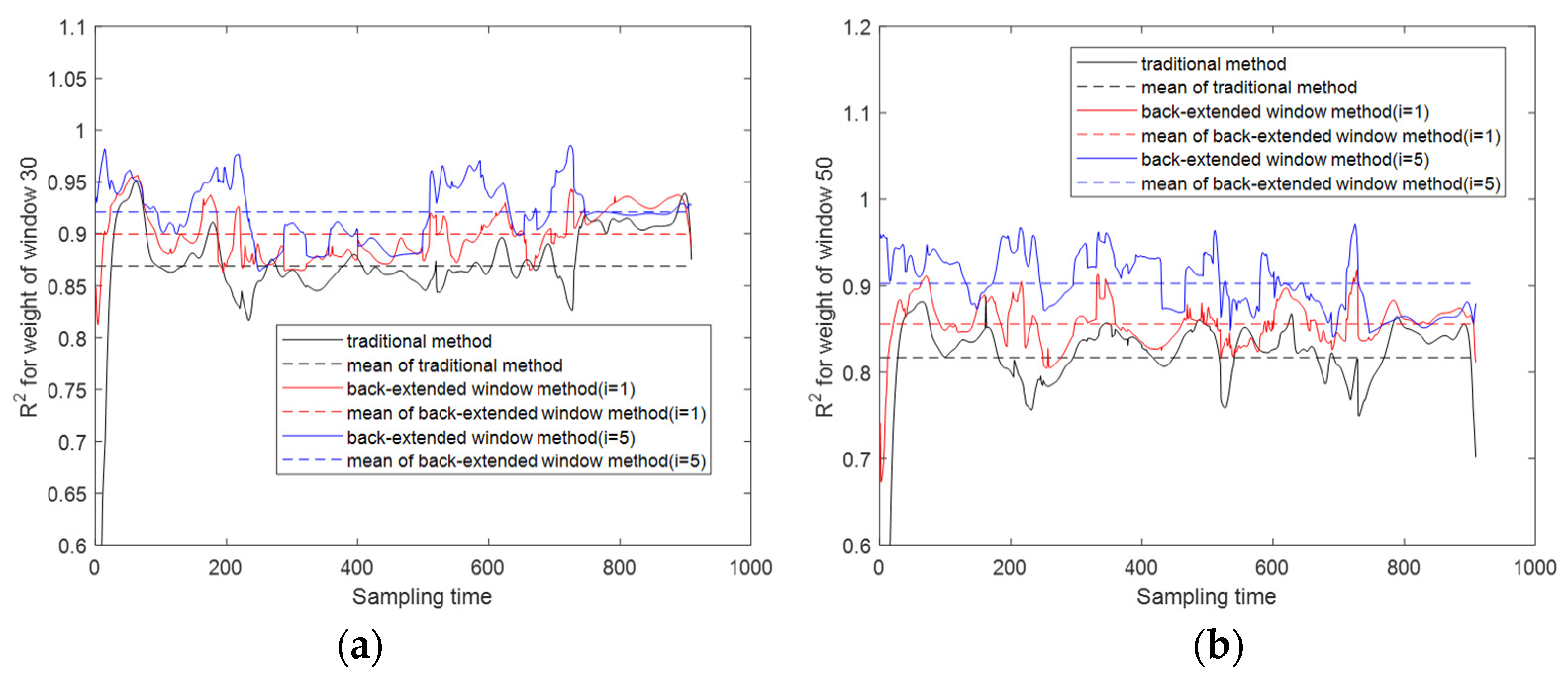
Window 30 and window 50 are also selected to give the

R_{k, c}^{2}

of each sampling point using the traditional method, backward extended window method with 1 extended batch, and backward extended window method with 5 extended batches. And the results are shown in Figure 7.

From Figure 7, compared with those of the traditional method, the

R_{k, c}^{2}

values of the model built through the back-extended window are improved; at the same time, when more batches are expanded, the

R_{k, c}^{2}

values of the model are better. This matches the conclusion obtained before, that is, the backward extension of the data at the sampling time can help to improve the prediction model; the benefits brought by the extension of the batch and the extension of the backward sampling times can also be superimposed.

3.3.5. Application of the k-i-Back-Extended Window Model

In this section, the rationality of the k-i-back-extended window based on the time-batch evolution information is verified. The sets of parameter combinations are listed in Table 6, and corresponding

\bar{R_{c}^{2}}

values are analyzed separately.

It can be seen from Table 6 that with the continuous extension of the data,

\bar{R_{c}^{2}}

continues to increase, which proves that the

\bar{R_{c}^{2}}

brought by the extension in the various directions discussed above can be continuously increased.

3.4. Online Quality Analysis and Prediction

Online quality prediction is conducted using the proposed model prediction method based on the time-batch evolution information. For better comparison, in addition to using the proposed k-i-back-extended window model, the traditional method, the k-extended window method, the i-extended window method, the k-i-extended window method and the back-extended window method are used to perform the task of quality prediction. The parameter settings for these experiments are shown in the table below.

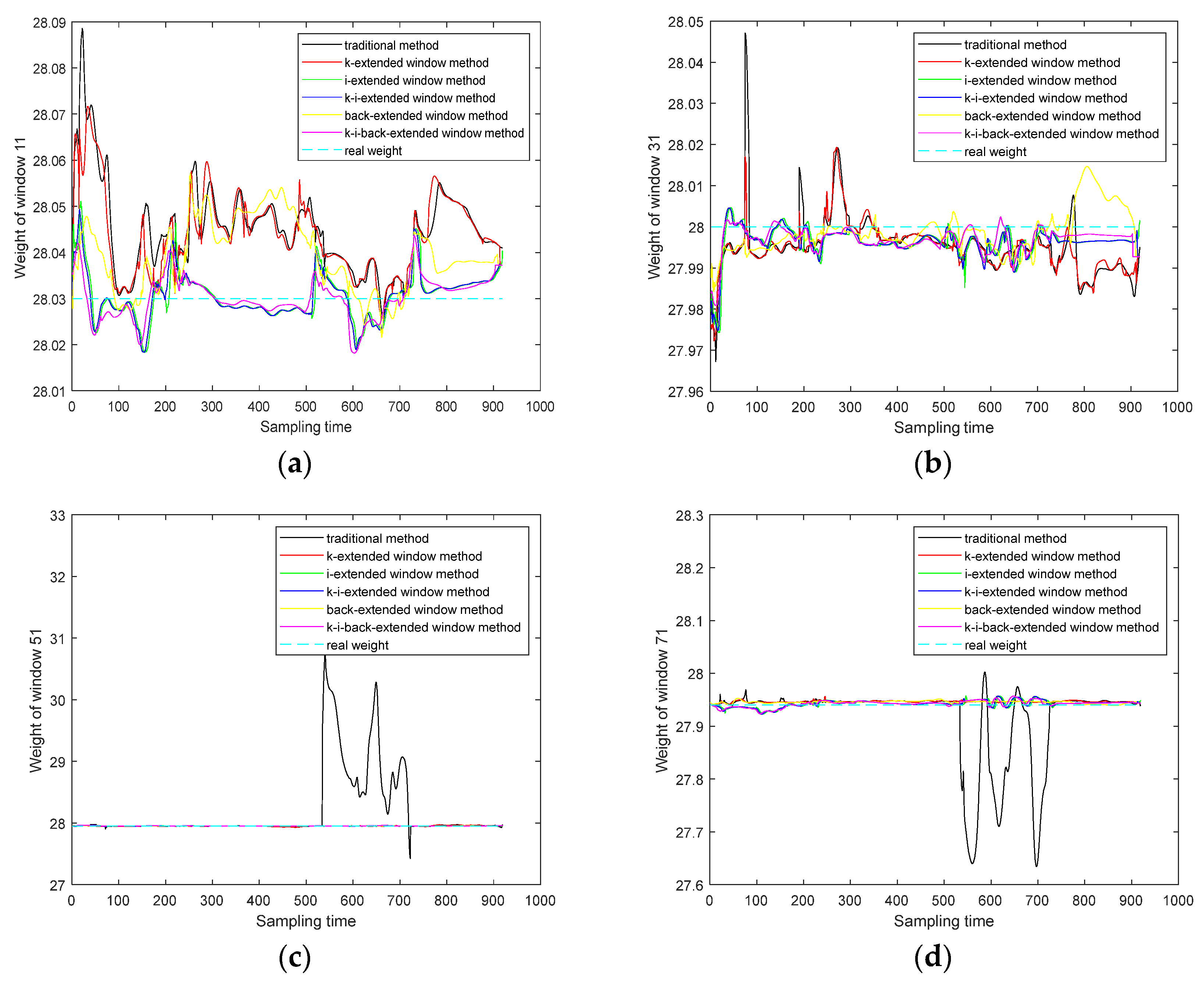
The analysis is also performed using the sliding windows, and the middle batch of each window is selected as the test batch to verify the accuracy of each prediction method. For the four test batches, the online quality prediction is performed, and the predicted results of weight obtained by the six methods at each sampling time are plotted in Figure 8.

It is easy to know from Figure 8 that the prediction performance of the traditional method is more unstable compared with the proposed methods based on extended windows, especially in window 51 and window 71, that is, the prediction methods of the four extended window models based on the proposed method are significantly better than the traditional method. To further understand the accuracy gained by the proposed four models, the mean RMSE values corresponding to all sampling times in each test batch are listed in Table 8.

It can be seen that in the above selected test batches, in general, the prediction method based on the k-i-back-extended window achieves the best results. The prediction method based on this kind of extended window has the lowest RMSE on average. In the 11th window, its RMSE indicator reaches a low value of 2.587×10^-4. In addition, it should be noted that by observing the four methods of each test batch, it is easy to see that in individual test batches, only the extension in the direction of the sampling time, RMSE can reach the lowest value. But obviously, this advantage is unstable. For example, in batch 31, the prediction model that only uses the sampling time to extend the window is not even as good as the traditional method; in other words, when only one-dimensional extension is performed the accuracy advantage may be only obtained in individual test batches. Based on the above, the effects of the five methods proposed in this paper on quality prediction have been proved.

Therefore, combining the

\bar{R_{c}^{2}}

index and

R_{k, c}^{2}

index obtained in the previous section, the following conclusions can be drawn: Firstly, compared with the traditional method, the extension in the direction of batches or in the direction of historical sampling time can achieve the purpose of improving the accuracy, and the extension in either the sampling time or batch directions is meaningful. Secondly, considering the evolution information of two directions in the model at the same time, establishing an extended window based on the time-batch evolution information of sampling in both directions can further improve the accuracy and effectively improve the stability of the prediction model. In addition, in the actual production process, several modeling methods based on the extended window proposed above are suggested. When the production is in pursuit of obtaining high-precision products quickly and easily, the one-dimensional extended window is recommended to be used; When the production accuracy requirement is very high, then the two-dimensional windows should be used to build quality prediction models.

4. Conclusions

This paper proposed a new quality prediction strategy for batch processes. In the proposed method, the newly defined ROSs are used to build five different extended windows, which contain the data information of historical batches and historical sampling times. The quality prediction models of these extended windows have richer batch-time operation evolution information, and the evolution information brings higher prediction accuracy. When all the sampled data in KIBROS is considered in the model, the k-i-back-extended window is established, and the highest accuracy is obtained in the application on the injection molding process. For complex production situations, when product quality accuracy is critical, the two-dimensional KIBROS extended window is recommended.

Author Contributions

Conceptualization, L.Z.; methodology, L.Z. and J.Y.; software, J.Y.; validation, J.Y.; formal analysis, J.Y.; investigation, J.Y.; resources, L.Z.; data curation, L.Z.; writing—original draft preparation, L.Z. and J.Y.; writing—review and editing, L.Z.; visualization, J.Y.; supervision, L.Z.; project administration, L.Z.; funding acquisition, L.Z. All authors have read and agreed to the published version of the manuscript.

Funding

This research was funded by the National Natural Science Foundation of China (No. 61503069) and the Fundamental Research Funds for the Central Universities (N150404020).

Conflicts of Interest

The authors declare no conflicts of interest.

References

Dunteman G. Principal Component Analysis; SAGE publication Inc.: 1989, Los Angeles.
Geladi P, Kowalshi B. Partial least squares regression: A tutorial. Anal. Chim. Acta. 1986, 185, 1–17. [CrossRef]
Wang X. Data mining and knowledge discovery for process monitoring and control; Springer: Berlin/Heidelberg, Germany, 1999.
Kourti T, MacGregor J. Process analysis, monitoring and diagnosis, using multivariate projection methods. Chemom. Intell. Lab. Syst. 1995, 28, 3–21. [CrossRef]
Wang H. Partial least squares regression method and its application; National Defense Industry Press: 1999, Beijing.
Nomikos P, MacGregor J. Monitoring batch processes using multiway principal component analysis. AIChE J. 1994, 40, 1361–1375. [CrossRef]
Nomikos P, MacGregor J. Multi-way partial least squares in monitoring batch processes. Chemom. Intell. Lab. Syst. 1995, 30, 97–108. [CrossRef]
Wold S, Kettaneh N, Fridén H, Holmberg A. Modelling and diagnostics of batch processes and analogous kinetic experiments. Chemom. Intell. Lab. Syst. 1998, 44, 331–340. [CrossRef]
Duchesne C, MacGregor J. Multivariate analysis and optimization of process variable trajectories for batch process. Chemom. Intell. Lab. Syst. 2000, 51, 125–137. [CrossRef]
Cho H, Kim K. A method for predicting future observations in the monitoring of a batch process. Qual. Technol. 2003, 35, 59–69. [CrossRef]
Lu N, Wang F, Gao F. Sub-PCA modeling and online monitoring strategy for batch processes. AIChE J. 2004, 50, 255–259. [CrossRef]
Zhao L, Zhao C, Gao F. Inter-batch-evolution-traced process monitoring based on inter-batch mode division for multi-phase batch processes. Chemom. Intell. Lab. Syst. 2014, 138, 178–192. [CrossRef]
Zhao L, Wang F, Chang Y, Wang S, Gao F. Phase-based recursive regression for quality prediction of multi-phase batch processes. In Proceedings of the 13th IEEE International Conference on Control and Automation, Ohrid, Macedonia, 3–6 July 2017, 283–288. [CrossRef]
Hwang D, Han C. Real-time monitoring for a process with multiple operating modes. Control Eng. Pract. 1999, 7, 891–902. [CrossRef]
Chen J, Liu J. Mixture principal component analysis models for process monitoring. Ind. Eng. Chem. Res. 1999, 38, 1478–1488. [CrossRef]
Zhao L, Zhao C, Gao F. Between-mode quality analysis based multi-mode batch process quality prediction. Ind. Eng. Chem. Res. 2014, 53, 15629–15638. [CrossRef]
Qin Y. Research on data driven batch process monitoring and quality control; Zhejiang University: Hangzhou, China, 2018.
Zhao, L, Huang, X, Yu, H. Quality-analysis-based process monitoring for multi-phase multi-mode batch processes. Processes 2021, 9, 1321. [CrossRef]
Luo L, Bao S, Gao Z, et al. Batch process monitoring with GTucker2 model. Ind. Eng. Chem. Res. 2014, 53(39), 15101–15110. [CrossRef]
Zhao, L, Yang, J. Batch process monitoring based on quality-related time-batch 2D evolution information. Sensors 2022, 22, 2235. [CrossRef]
You L X, Chen J. Autogenerated multilocal PLS models without pre-classification for quality monitoring of nonlinear processes with unevenly distributed data. Ind. Eng. Chem. Res. 2022. 16(17), 5898–5913. [CrossRef]
Zou M, Zhao L, Wang S, et al. Quality analysis and prediction for start-up process of injection molding processes. IFAC-PapersOnLine, 2018, 51(18), 233–238. [CrossRef]
Guo X, Lu N, Gao F, Wang F. Sliding window sub-phase PCA modeling and online monitoring of batch process. Control and Decision, 2005(09), 1034–1037.
Yao Y, Lu N, Gao F. Two-dimensional dynamic PCA with auto-selected support region. IFAC Proceedings Volumes, 2007, 40(5). [CrossRef]
Jia R, Mao Z, Wang F. KPLS model based product quality control for batch processes. CIESC Journal, 2013, 64(4), 1332–1339. [CrossRef]

Figure 1. Schematic diagram of sliding window.

Figure 2. Schematic diagram of novel ROS.

Figure 3. Backward extension in the direction of batch.

Figure 4. A schematic diagram of the injection molding machine.

Figure 5. based on the KROS in (a) sliding window 30 and (b) sliding window 50.

Figure 6. based on the IROS and KIROS in (a) sliding window 30 and (b) sliding window 50.

Figure 7. based on the BROS in (a) sliding window 30 and (b) window 50.

Figure 8. Predicted results of each sampling time in (a) sliding window 11, (b) sliding window 31, (c) sliding window 51, and (d) sliding window 71.

Table 1. Process variables of the injection molding process.

No.	Variable description	Unit
1	Nozzle temperature	℃
2	Screw speed	Mm/s
3	Cylinder pressure	Bar
4	Plasticizing pressure	Bar
5	SV1 valve opening	%
6	SV2 valve opening	%

Table 2. Operating condition settings for the injection molding process.

Operating parameter	Set value
Material	High density polyethylene (HDPE)
Injection velocity	24 mm/sec
Packing pressure	200 bar
Mold cooling water	25℃
Barrel temperature	230℃
Packing time	3 s
Cooling time	15 s

Table 3. based on the k-extended window.

F	Phase 1	Phase 2	Phase 3	Phase 4	Whole
0	0.6674	0.6701	0.7236	0.7551	0.7031
1	0.6735	0.6718	0.7284	0.7590	0.7116
2	0.6784	0.6739	0.7316	0.7621	0.7149
3	0.6834	0.6760	0.7349	0.7648	0.7177
4	0.6881	0.6779	0.7378	0.7668	0.7202
5	0.6924	0.6794	0.7408	0.7687	0.7224
6	0.6961	0.6805	0.7438	0.7699	0.7244
7	0.6993	0.6813	0.7470	0.7709	0.7264
8	0.7021	0.6820	0.7500	0.7714	0.7282
9	0.7046	0.6826	0.7529	0.7718	0.7299
10	0.7068	0.6833	0.7557	0.7720	0.7315

Table 4. based on the k-extended window and k-i-extended window.

F	N	Phase 1	Phase 2	Phase 3	Phase 4	Whole
0	0	0.6674	0.6701	0.7236	0.7551	0.7031
	1	0.7125	0.6948	0.7781	0.7727	0.7281
	2	0.7620	0.7526	0.8180	0.8193	0.7596
	3	0.7951	0.8070	0.8458	0.8323	0.7934
	4	0.8359	0.8280	0.8686	0.8445	0.8129
	5	0.8585	0.8591	0.8911	0.8641	0.8332
	6	0.8723	0.8795	0.8915	0.8788	0.8468
	7	0.8903	0.8879	0.7827	0.9014	0.8576
	8	0.9011	0.9063	0.8121	0.9119	0.8709
	9	0.9098	0.9165	0.8271	0.9203	0.8804
	10	0.9192	0.9196	0.8392	0.9252	0.8850
6	0	0.6961	0.6805	0.7438	0.7699	0.7244
	1	0.7343	0.6987	0.7977	0.7904	0.7409
	2	0.7785	0.7578	0.8393	0.8313	0.7699
	3	0.8088	0.8115	0.8652	0.8419	0.8033
	4	0.8465	0.8321	0.8841	0.8538	0.8214
	5	0.8669	0.8628	0.9050	0.8726	0.8409
	6	0.8799	0.8830	0.9023	0.8863	0.8540
	7	0.8974	0.8910	0.7886	0.9085	0.8649
	8	0.9072	0.9095	0.8175	0.9178	0.8778
	9	0.9154	0.9193	0.8312	0.9256	0.8868
	10	0.9246	0.9223	0.8423	0.9295	0.8913

Table 5.

\bar{R_{c}^{2}}

based on the back-extended window.

Table 5.

\bar{R_{c}^{2}}

based on the back-extended window.

F	B	Phase 1	Phase 2	Phase 3	Phase 4	Whole
1	0	0.7125	0.6948	0.7781	0.7727	0.7281
	1	0.7084	0.6903	0.7745	0.7678	0.7268
	2	0.7062	0.6873	0.7726	0.7659	0.7273
	3	0.7044	0.6851	0.7719	0.7662	0.7279
	4	0.7050	0.6836	0.7718	0.7682	0.7288
	5	0.7069	0.6829	0.7721	0.7702	0.7299
	6	0.7093	0.6827	0.7724	0.7724	0.7311
	7	0.7117	0.6829	0.7729	0.7743	0.7322
	8	0.7140	0.6833	0.7735	0.7759	0.7334
	9	0.7162	0.6841	0.7741	0.7773	0.7343
	10	0.7179	0.6849	0.7748	0.7782	0.7349
5	0	0.8585	0.8591	0.8911	0.8641	0.8332
	1	0.8503	0.8528	0.8890	0.8564	0.8277
	2	0.8467	0.8482	0.8879	0.8529	0.8251
	3	0.8450	0.8460	0.8875	0.8507	0.8244
	4	0.8443	0.8448	0.8879	0.8488	0.8245
	5	0.8443	0.8442	0.8885	0.8471	0.8250
	6	0.8449	0.8439	0.8897	0.8455	0.8257
	7	0.8460	0.8439	0.8910	0.8443	0.8266
	8	0.8475	0.8441	0.8925	0.8432	0.8275
	9	0.8493	0.8444	0.8941	0.8422	0.8285
	10	0.8512	0.8448	0.8957	0.8414	0.8296

Table 6. Sets of parameter combinations and corresponding

\bar{R_{c}^{2}}

Table 6. Sets of parameter combinations and corresponding

\bar{R_{c}^{2}}

No.	F	N	B	$\bar{R_{c}^{2}}$
1	0	0	0	0.6539
2	6	0	0	0.6827
3	0	5	0	0.8493
4	0	1	6	0.6941
5	6	5	0	0.8584
6	6	1	6	0.7229
7	0	5	6	0.8376
8	6	5	6	0.8646

Table 7. Quality prediction method used for comparison.

Method	F	N	B
traditional	0	0	0
k-extended window	6	0	0
i-extended window	0	5	0
k-i-extended window	6	5	0
back-extended window	0	1	10
k-i-back-extended window	6	5	10

Table 8. Comparison of RMSE gained by the different prediction methods.

Method	Batch 11	Batch 31	Batch 51	Batch 71	Mean
traditional	0.0151	0.0046	0.2318	0.0224	0.0685
k-extended window	0.0141	0.0049	0.0016	0.0064	0.0068
i-extended window	6.516×10^-4	0.0037	0.0031	0.0027	0.0025
k-i-extended window	5.403×10^-4	0.0037	0.0032	0.0027	0.0025
back-extended window	0.0092	0.0014	0.0031	0.0055	0.0048
k-i-back-extended window	2.587×10^-4	0.0031	0.0039	0.0024	0.0024

Disclaimer/Publisher’s Note: The statements, opinions and data contained in all publications are solely those of the individual author(s) and contributor(s) and not of MDPI and/or the editor(s). MDPI and/or the editor(s) disclaim responsibility for any injury to people or property resulting from any ideas, methods, instructions or products referred to in the content.

© 2024 by the authors. Licensee MDPI, Basel, Switzerland. This article is an open access article distributed under the terms and conditions of the Creative Commons Attribution (CC BY) license (http://creativecommons.org/licenses/by/4.0/).

Copyright: This open access article is published under a Creative Commons CC BY 4.0 license, which permit the free download, distribution, and reuse, provided that the author and preprint are cited in any reuse.

MDPI Initiatives

Important Links

Choose an area of interest and we will send you notifications of new preprints at your preferred frequency.

Disclaimer

High-precision Quality Prediction Based on Two-dimensional Extended Windows

Abstract

1. Introduction

2. Methodology

2.1. Partial Least Squares Method (PLS)

2.2. Establishment of Sliding Window

2.3. Two-Dimensional Extended ROS

2.4. Quality Prediction Method and Evaluation Indicators

3. Illustration and Discussions

3.1. Introduction of Injection Molding Process

3.2. Variable Analysis of Injection Molding Process and Experiment Condition

3.3. Application of Prediction Model and Identification of Related Parameters

3.3.1. Application of One-Dimensional Extended Window Model Using the Samples in KROS Only

3.3.2. Application of Extended Window Model Using the Samples in IROS and KIROS

3.3.3. Application of Extended Window Prediction Model Using the Samples in BROS

3.3.5. Application of the k-i-Back-Extended Window Model

3.4. Online Quality Analysis and Prediction

4. Conclusions

Author Contributions

Funding

Conflicts of Interest

References

MDPI Initiatives

Important Links

Subscribe