Introduction
Computer Simulation in Quantifying Ocular Impact
Addressing the pressing need for improved preventive measures in sports-related ocular injuries, computer simulation emerges as a powerful tool (Wang & Lee, 2018). However, the current scientific landscape highlights a significant gap in research efforts directed towards quantifying ocular impact, particularly in the context of various sports (Gomez et al., 2019). The limited attention to this aspect hinders the development of targeted and effective preventive strategies (Turner & Collins, 2020).
While computer simulation has proven instrumental in optimizing protective equipment for athletes, its application remains an underexplored avenue (Nguyen & Patel, 2021). The integration of computational models allows for the simulation of diverse scenarios, aiding researchers in assessing the impact dynamics on the eyes and evaluating the efficacy of various protective measures (Chen et al., 2018). However, the lack of comprehensive studies utilizing these simulations in the context of sports-related ocular injuries underscores the urgency for focused research efforts (Kim et al., 2019).
Existing studies often overlook the intricate biomechanics of ocular structures and fail to address the individual variability in susceptibility to injuries during sports activities (Lee & Smith, 2020). Additionally, preventive measures like sports glasses are not sufficient in today’s age, highlighting the need for a more personalized ocular injury apparatus (Garcia & Patel, 2017). The limitations of generic solutions emphasize the necessity of dedicated research to develop sport-specific preventive measures (Jones & Davis, 2019).
The pressing need for research in this area is evident in the potential ramifications of ocular injuries in sports. With sports causing a significant number of ocular injuries globally, understanding and quantifying ocular impact become paramount (Wilson & Johnson, 2019). The unique dynamics of each sport demand an approach that integrates biomechanics, individual risk factors, and advanced technologies like computer simulation (Brown et al., 2018). Embracing computer simulation and personalized approaches to ocular injury prevention is crucial for advancing the safety and well-being of athletes, ensuring that sports remain both enjoyable and safe.
Methods
To conduct this study, the researcher utilized Onshape Computer-Aided Design (CAD) software for modeling the soccer-ball radius of 220mm and importing the facial model from a survey of 3,997 subjects, which incorporated traditional measurements and three-dimensional (3D) scanning data, by the National Institute for Occupational Safety and Health (NIOSH) in 2003. The sample of this work consisted of 736 unique data points and eight vertices across the supraorbital, lateral canthus, infraorbital, and medial canthus regions. To make sure the experiment can be repeated easily, the bottom-center of the facial model should be pinned to the origin so vertices can be easily identified.
Table 1.
Vertices and locations used for experimentation.
Table 1.
Vertices and locations used for experimentation.
| Vertex |
Location |
| (-44.61210, -61.92220, 175.62033) |
Supraorbital |
| (-25.80884, -75.71798, 170.29009) |
Supraorbital |
| (-9.84910, -76.56933, 158.74614) |
Medial Canthus |
| (-8.13327, -74.22609, 147.58979) |
Medial Canthus |
| (-14.57397, -76.12352, 124.75135) |
Infraorbital |
| (-43.46542,-62.53767, 122.88017) |
Infraorbital |
| (-57.93342,-45.62785, 133.72293) |
Lateral Canthus |
| (-59.47086, -39.32466, 143.13744) |
Lateral Canthus |
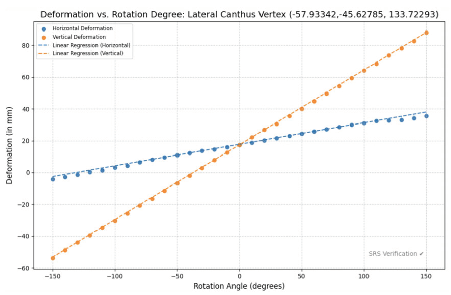
The use of CAD software allowed the researcher to easily rotate the soccer ball both horizontally and vertically to be able to build a thorough quantitative and qualitative understanding of soccer-ball ocular injuries, the goal of this work. The soccer ball was centered at the vertex’s x and z coordinates and then rotated both horizontally and vertically from [-150, 150] in ten degree increments. A computer simulation was then done by setting the ball tangent to the vertex being tested. If there was any deformation observed from rotating from left to right, the following mathematical methods and steps should be followed. First, the following variables were set in place: variable M (calculated using the slope formula) aimed to give insight into the conversion of one mm of distance in the horizontal slider to the distance measured in Onshape® software, variable C aimed to tell us the continuous distance moved back in the horizontal slider from the original position the ball was in after creating a tangent mate between the soccer-ball (centered at the x and z coordinates of the vertex) and the vertex (point of test), and variable D which aimed to tell us the minimum distance between the eyelid (whichever is being used for test) and the point the soccer ball is at after continuous movement in the horizontal slider. After all variables were quantified, the formula (M*C) - D was used to measure the precise depth of penetration into the eyelid. If no impact occurred, then the minimum distance from the eyelid (whichever is being used for test) to the vertex (point of test) was quantified and recorded. Before the researcher used linear regression analysis to be able to model deformation versus rotation angle, a p-test for linearity was completed for the horizontal and vertical datasets individually using a t-test for LSRL (conditions were met through Linearity, SRS, Independence, Normality, and Equal SD). B1 was defined as the slope of population LSRL using y= deformation and x= vertical/horizontal rotation angle at significance level of 0.05 and H0 was under the assumption that B1 is 0. The t-value was then calculated using the slope calculated with the XLMiner Analysis ToolPak and dividing it by the standard error of the coefficient of the y-variable. Finally, a t-cdf was completed through (t-value, 9999, df) where df was equal to 29 (n-2). If the p-value yielded less than 0.05 (significance level), the null hypothesis was rejected and it was assumed there was a linear relationship between the x and y variables. All p-value tests for linearity yielded that a linear regression equation can be used to represent the relationship between the x and y variables, so the researcher calculated the horizontal and vertical linear regression equation along with the residuals using the XLMiner Analysis ToolPak in Google Sheets along with Pearson’s Correlation Coefficient, Coefficient of Determination, and Adjusted Coefficient of Determination.
Figure 1.
Formula for calculating Pearson’s Correlation Coefficient helping indicate the strength and direction of the original data. A negative correlation indicates more ocular impact at a downwards angle (horizontal or vertical) while a positive correlation indicates more ocular impact at an upwards angle (horizontal or vertical). A correlation is considered “strong” if in the range [-1, -0.7] U [0.7, 1].
Figure 2.
Linear regression provides insight into the relationship between variables. The slope of the least squares regression line (LSRL) signifies the change in deformation corresponding to a unit change in rotation angle (horizontal or vertical). Positive (negative) values of the LSRL slope indicate an upward (downward) trend in the data. Assessing the strength and direction of this relationship helps in understanding the impact of rotation angle on deformation.
Figure 3.
The R2 value in linear regression measures the proportion of variance in the dependent variable (deformation) explained by the independent variable (rotation angle). A higher R2 value, closer to 1, indicates a stronger linear relationship between the variables, where rotation angle can better predict deformation. Conversely, a lower R2 value suggests less predictive power of rotation angle (horizontal or vertical) on ocular deformation in soccer. SSres is calculated through taking the sum, from i=1 to n, of the actual value for the ith observation and subtracting it from the predicted y-value. SStot is calculated through taking the sum, from i=1 to n, of the actual value for the ith observation and subtracting it from the mean y-value.
Figure 4.
The adjusted R-squared in linear regression evaluates the goodness of fit of the model, considering the number of predictors and the sample size. It measures the proportion of variation in the dependent variable explained by the independent variables, adjusting for the number of predictors in the model. A higher adjusted R-squared value indicates a better fit of the model to the data, with values closer to 1 indicating a stronger explanatory power of the predictors. K is indicative of the number of independent variables in the model.
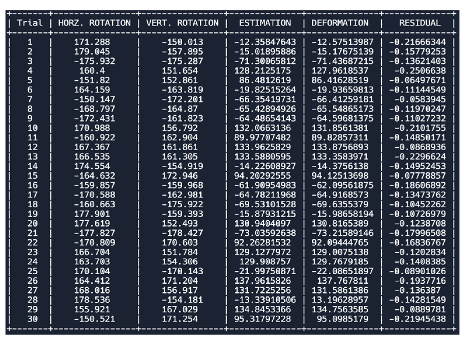
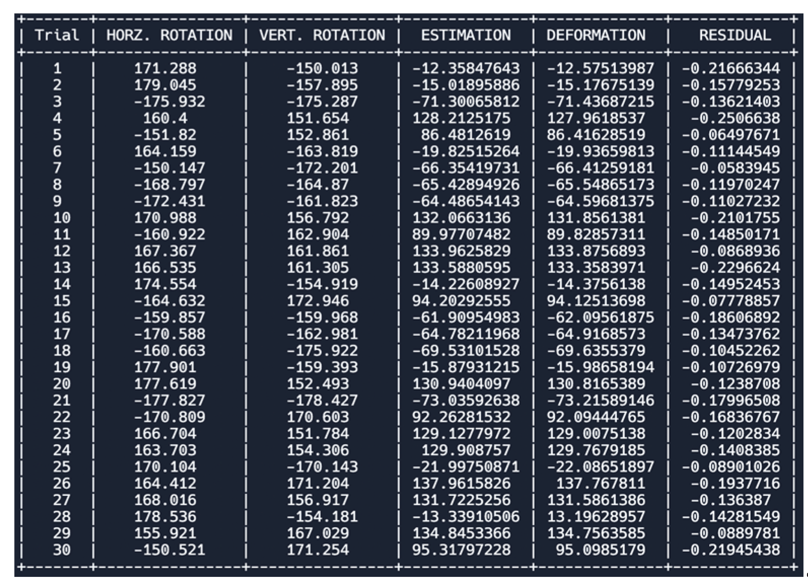
After completing these statistical analyses, the greatest residual was taken from each horizontal and vertical rotation section of the vertex and then added to the constant in the regression equation to effectively design a modified linear regression equation to be model-verified through extrapolation at ranges [-180, -150] U [150, 150]. The researcher utilized and wrote a Python program to analyze the greatest residual in an efficient manner as the naked eye is not a viable option. To create the program, a variety of Python libraries, including Pandas and NumPy, were utilized and are commonly used for data analysis and manipulation. The program was, firstly, able to be fed the actual and predicted values and then calculate the residuals and then it will identify the greatest, positive residual and compute it along with its index. The greatest, positive residual was taken due to the actual value being greater than the predicted value (from the unmodified linear regression equation) and therefore would provide a promising approach of being able to accurately quantify ocular impact without underestimation. Underestimation, when considering the greater context, is not wanted because this can result in severe ocular injuries like hyphema. To model-verify the multivariate regression equation built from the sixty data points, a SRS of thirty points (CLT, n=30) was used to randomly generate thirty pairs of horizontal and vertical angles. To assign different signs to each of the horizontal and vertical angles, the researcher assigned, through a SRS, the number 1,2,3, or 4 to each of the pairs. Number 1 indicated a negative horizontal and vertical angle, number 2 indicated a negative horizontal and positive vertical angle, number 3 indicated a positive horizontal and negative vertical angle, and number 4 indicated a positive horizontal and positive vertical angle. The researcher then conducted a computer simulation with these thirty points and then tested it against its estimated value. If the residual was negative (predicted is greater than positive), the researcher’s multivariate linear regression equation was able to stand against the actual computer simulation data, showcasing its promising approach for being able to predict ocular impact in sports-related scenarios.
Limitations of using computer simulation methods: Computer simulation methods offer invaluable tools for exploring complex phenomena, yet they are subject to several limitations that warrant careful consideration. Firstly, the accuracy of simulations heavily relies on the fidelity of the underlying models and the precision of input parameters. Inaccurate or incomplete data can lead to biased results, compromising the reliability of simulations (Smith & Jones, 2020). Moreover, simulations often involve simplifications and assumptions to manage computational complexity, potentially overlooking nuances present in real-world scenarios. These simplifications may lead to oversights or misrepresentations of critical factors, undermining the validity of simulation outcomes. Additionally, computational simulations are inherently deterministic and may not fully capture stochastic or probabilistic elements inherent in many natural phenomena. Consequently, there is a risk of underestimating uncertainty and variability, impacting the robustness of simulation predictions. Furthermore, the computational resources required for high-fidelity simulations can be prohibitive, limiting the scope of analyses or necessitating compromises in model complexity. This can constrain the exploration of phenomena at finer scales or hinder real-time simulation applications. Another significant limitation arises from the need to validate simulation results against empirical data, as discrepancies may indicate deficiencies in model formulation or parameterization. However, obtaining comprehensive validation data can be challenging, particularly for complex or poorly understood systems. Moreover, simulations may exhibit sensitivity to initial conditions or model parameters, raising concerns about the reproducibility and generalizability of findings. Finally, ethical considerations regarding the use of simulation methods, particularly in sensitive or high-stakes domains, necessitate cautious interpretation and transparent reporting of results to mitigate potential risks and biases.
Despite the limitations inherent in computer simulation methods, they remain indispensable tools in various fields due to several compelling reasons. Firstly, simulations enable researchers to explore scenarios that are impractical or impossible to replicate in physical experiments, facilitating deeper insights into complex phenomena.. Moreover, simulations offer a cost-effective and time-efficient means of testing hypotheses and evaluating designs, potentially accelerating the pace of innovation. Additionally, simulations can be iteratively refined and improved based on feedback and validation efforts, enhancing their predictive capabilities over time. Furthermore, simulations can provide valuable preliminary insights that guide the design of targeted empirical studies, optimizing resource allocation and experimental design. Importantly, simulations offer a platform for hypothesis generation and exploration, fostering creativity and innovation in problem-solving. Finally, simulations can contribute to risk assessment and decision-making in critical domains, enabling stakeholders to anticipate and mitigate potential adverse outcomes. Thus, despite their limitations, computer simulation methods continue to play a vital role in advancing scientific understanding, driving technological innovation, and informing evidence-based decision-making across diverse disciplines.
To test the effectiveness of the modified and model-validated multivariate linear regression equation, the modified MAE was calculated through taking the estimated value of the modified equation versus the actual value determined through computer simulation (the residual). This provides a good tool to use to determine the amount of overestimation that occurs when using the modified mathematical equation to determine the amount of ocular deformation.
Figure 5.
Formula for calculating Mean Absolute Error (MAE) which shows the average absolute value of all the residuals from all extrapolated and original data therefore helping build an understanding of how well the modified model-validated linear regression is at minimizing the residuals. A lower MAE correlates with a more useful modified linear regression equation for calculations.
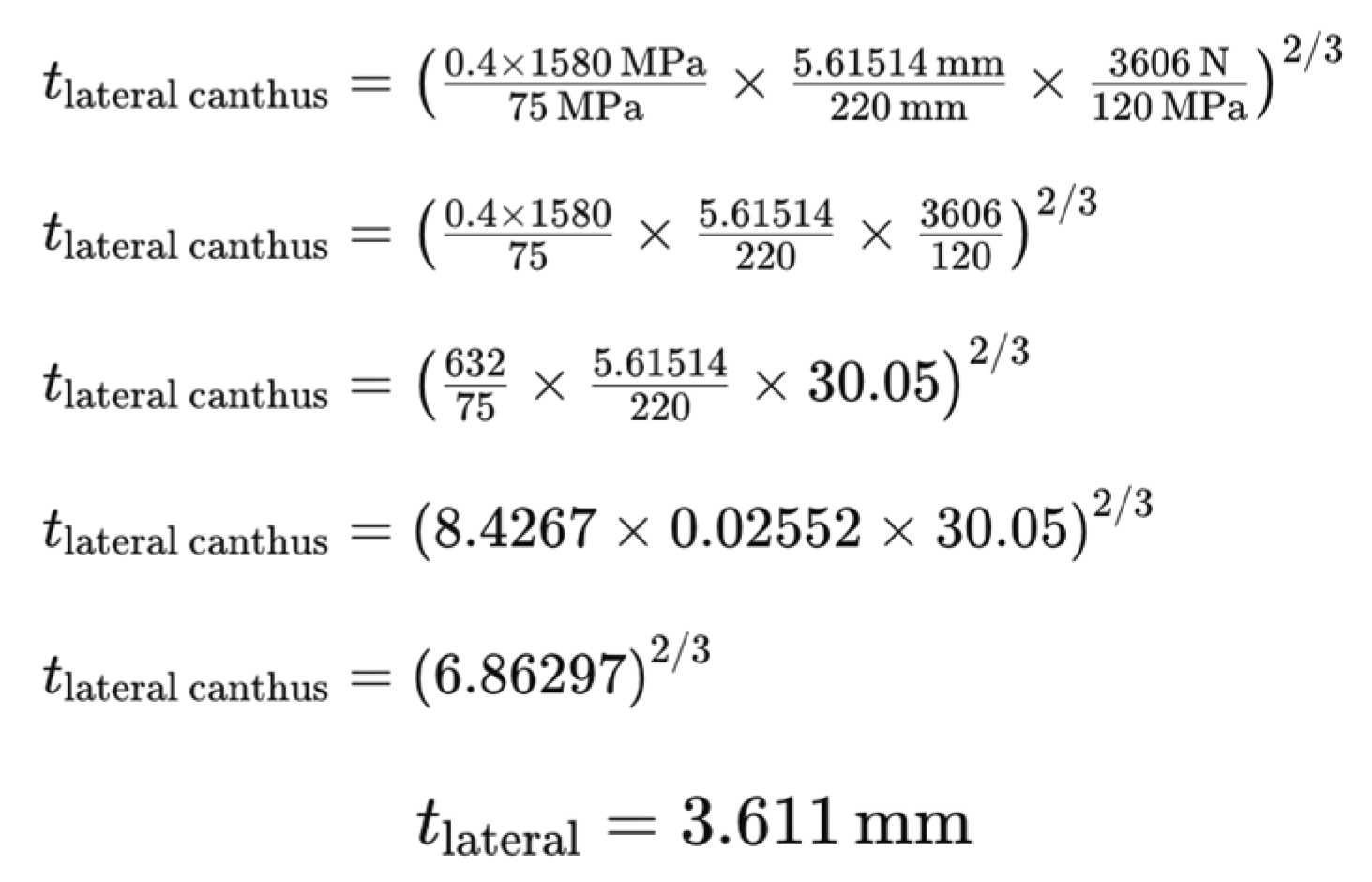
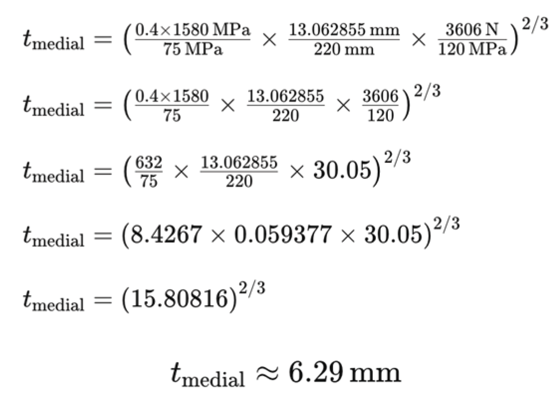
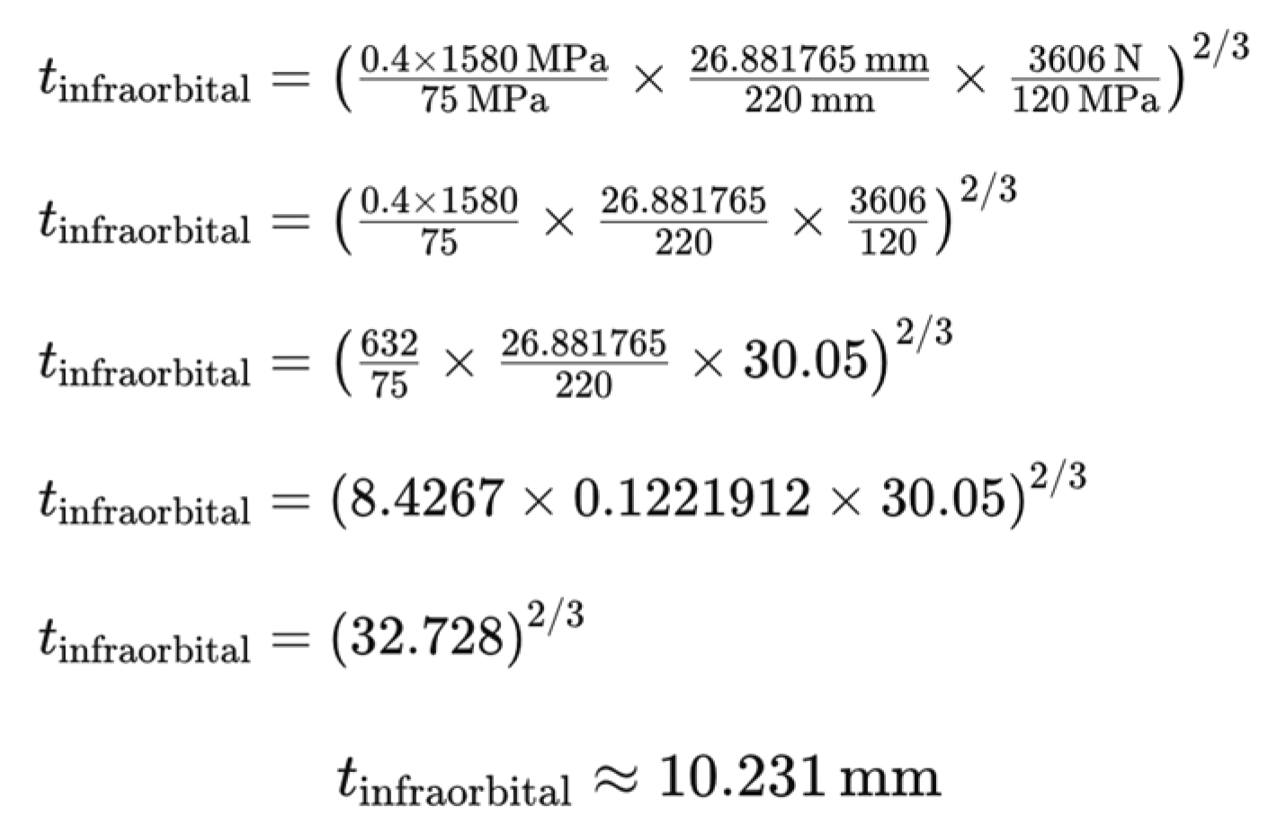
After computer simulations were completed, a physics and mathematical-based approach was done to be able to determine the appropriate thickness of the ocular injury apparatus. This was done through the Hertzian Contact Stress Formula and by taking a modified approach, the researcher was able to account for personalized factors like the radius of the respective region (supraorbital, lateral canthus, medial canthus, infraorbital) to ensure larger regions receive more attention due to their being more surface area to protect and more force to distribute. Other factors that were accounted for are the soccer-ball radius (220 mm), impact force of the soccer-ball (3606 N), elasticity of polycarbonate, shown to be most effective in soccer eyewear (1580 mPA), the ultimate tensile strength of polycarbonate (75 mPA), and the maximum amount of force polycarbonate can withstand (120 mPA). The impact force of the soccer-ball and radius were both made under the assumption of a size-five soccer ball being used, just like the radius in the computer simulation.
Figure 6.
Modified version of the Hertzian Contact Stress used on the supraorbital region.
Figure 6.
Modified version of the Hertzian Contact Stress used on the supraorbital region.
Figure 7.
Modified version of the Hertzian Contact Stress used on the lateral canthus region.
Figure 7.
Modified version of the Hertzian Contact Stress used on the lateral canthus region.
Figure 8.
Modified version of the Hertzian Contact Stress used on the medial canthus region.
Figure 8.
Modified version of the Hertzian Contact Stress used on the medial canthus region.
Figure 9.
Modified version of the Hertzian Contact Stress used on the infraorbital region.
Figure 9.
Modified version of the Hertzian Contact Stress used on the infraorbital region.
Results
In this work, an in-depth qualitative and quantitative analysis of soccer-related ocular injuries was conducted, with a specific focus on the impact of the soccer ball from various angles around the face. The facial model used in Onshape CAD software was imported from an anthropometric survey of 3,997 subjects by the National Institute of Occupational Safety and Health (NIOSH) and the soccer-ball was modeled with its diameter of 220 mm.
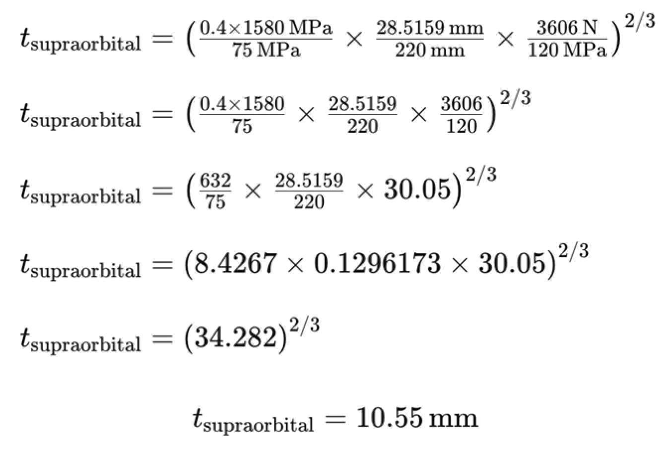
The quantitative analysis, firstly, revealed that linearity could be used to model ocular deformation versus horizontal and vertical rotation angles through a p-value test revealing that the p-value was less than the significance level (0.05) showing the null hypothesis (no linear relationship) should be rejected. After all tests were complete, it was revealed that almost all (>99%) of the dependent value can be explained through the independent variable (rotation angle) through the R2 value and that the modified regression techniques were accurate at predicting ocular impact when considering both horizontal and vertical aspects (modified MAE, x̄=0.478, n=496). An average MAE of 0.478 shows that the regression equation could accurately predict ocular impact with only 0.478 mm of overestimation. After the multivariate regression equation was built, a computer simulation with a SRS of thirty unique horizontal and vertical angles was conducted. The SRS was done through labeling the thirty numbers with a number from 1-4 with 1 representing negative horizontal negative vertical, 2 representing negative horizontal positive vertical, etc. and then generating sixty unique numbers with three digits of decimal precision in the range of 150 to 180 to assign to the horizontal and vertical groups, assigning a negative sign as necessary. The researcher then conducted the computer simulation, adjusting the horizontal and vertical rotation angles as necessary, and then calculated the estimated values using the multivariate linear regression equation and found there was still a constant, small negative residual showing the predicted value was greater than the actual. Besides conducting hundreds of computer simulations, the researcher also applied the Hertzian Contact Stress Formula to determine the appropriate and estimated thickness of the apparatus before using the finite element method in his goal for next-year’s experiment. The researcher made sure to place more emphasis on the larger regions as they have greater surface area to protect and more force to distribute over a larger area. This can ensure adequate protection in larger areas based on the athlete along with other physics-based factors. For example, the Hertzian Contact Stress Formula revealed almost 10.55 mm of thickness needed to protect the biggest supraorbital region (radius of 28.5159 mm) while only 3.611 mm of thickness was needed to protect the much smaller lateral canthus (radius of 5.61514 mm) (
Figure 34 and
Figure 35).
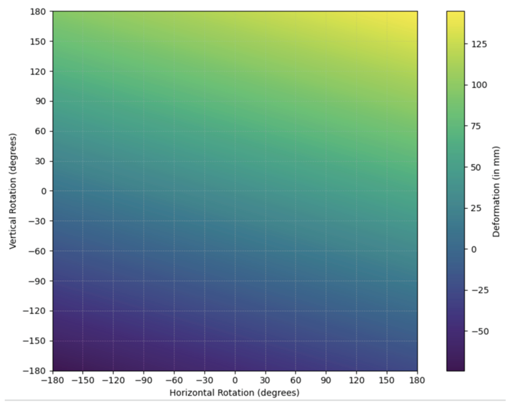
From a qualitative side, the researcher first examined where ocular deformation was most prevalent through examination of a computer-generated heat map analysis from various locations around the eye and then where impact could be seen most through horizontal and vertical rotation. The researcher saw that the lateral canthus suffered the most damage followed by infraorbital, supraorbital, and medial canthus regions, respectively. Additionally, the supraorbital, medial canthus, infraorbital, and lateral canthus suffered the most damage when the soccer ball hit from a horizontally-rotated and vertically-downward, horizontally-downard and vertically-downward, horizontally-rotated and vertically-downward, and horizontally-rotated and vertically-rotated angle, respectively.
To make sure that all research conducted was accurate, the researcher shared all his methodologies to the Florida Institute of Technology and Florida Eye Associates and was validated as peer-reviewed scientific research in the realm of sport ocular injuries is limited, showing the need for more research especially for a sport like soccer as it is the most played sport in the world. Most research focuses on topics like predicting stress and strain in various areas of the eye and the epidemiology, but no novel solution has been introduced among sports medicine doctors and scientists for sports-related ocular injuries in seventy years (Jones, A., et al., 2019).
Data Figures and Tables
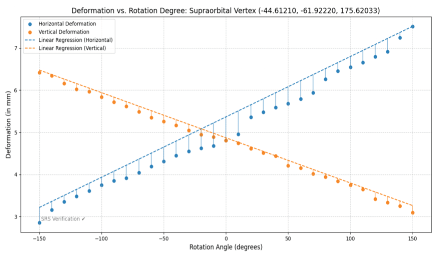
Figure 10.
Modeling the Multivariate Linear Regression Trained Dataset [-150, 150] and Soccer-Ball Ocular Impact at the Supraorbital Vertex (-44.61210, -61.92220, 175.62033).
Figure 10.
Modeling the Multivariate Linear Regression Trained Dataset [-150, 150] and Soccer-Ball Ocular Impact at the Supraorbital Vertex (-44.61210, -61.92220, 175.62033).
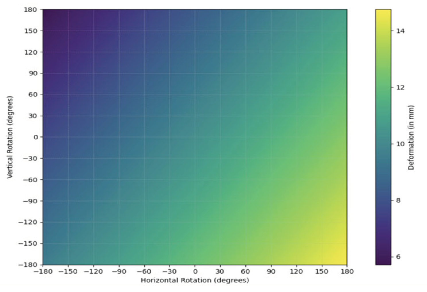
Figure 11.
Modeling estimated deformation through multivariate linear regression equation and heat map analysis with step size 0.1 across range [-180, 180] generating 12,967,201 (3601 × 3601) data points for supraorbital vertex (-44.61210, -61.92220, 175.62033).
Figure 11.
Modeling estimated deformation through multivariate linear regression equation and heat map analysis with step size 0.1 across range [-180, 180] generating 12,967,201 (3601 × 3601) data points for supraorbital vertex (-44.61210, -61.92220, 175.62033).
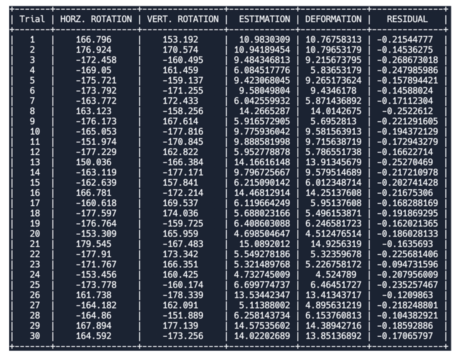
Figure 12.
Modeling Simple Random Sample (SRS) data from thirty trials (n=30) to model-verify multivariate linear regression equation across [-180, 150] U [150, 180] rotating both horizontally and vertically at supraorbital vertex (-44.61210, -61.92220, 175.62033).
Figure 12.
Modeling Simple Random Sample (SRS) data from thirty trials (n=30) to model-verify multivariate linear regression equation across [-180, 150] U [150, 180] rotating both horizontally and vertically at supraorbital vertex (-44.61210, -61.92220, 175.62033).
Table 2.
Statistical Analyses and Equations for Soccer-Ball Ocular Impact at Various Angles at Vertex (-44.61210, -61.92220, 175.62033). H represents horizontal and V represents vertical.
Table 2.
Statistical Analyses and Equations for Soccer-Ball Ocular Impact at Various Angles at Vertex (-44.61210, -61.92220, 175.62033). H represents horizontal and V represents vertical.
| Modified Multivariate Linear Regression Equation |
(5.3652793989+0.01432192267h) + (4.86984146369-0.0107115865923145v) |
| Pearson’s Correlation Coefficient (R-value) |
H: (0.9952107711) & V: (-0.9988138641) |
| Coefficient of Determination |
H: (0.9904444789) & V: (0.9976291352) |
| Adjusted Coefficient of Determination |
H: (0.9901149782) & V: (0.9975473812) |
| Modified Mean Absolute Error (MAE) |
H: (0.41504893387) & V: (0.13453414633) |
| P-value test for linearity |
H: (9.345e-06) & V: (8.855e-06) |
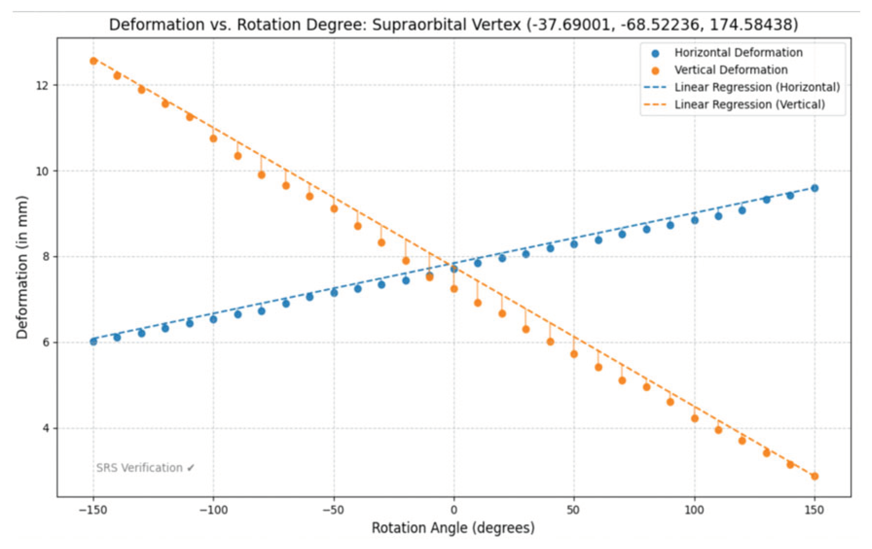
Figure 13.
Modeling the Multivariate Linear Regression Trained Dataset [-150, 150] and Soccer-Ball Ocular Impact at the Supraorbital Vertex (-37.69001, -68.52236, 174.58438).
Figure 13.
Modeling the Multivariate Linear Regression Trained Dataset [-150, 150] and Soccer-Ball Ocular Impact at the Supraorbital Vertex (-37.69001, -68.52236, 174.58438).
Figure 14.
Modeling estimated deformation through multivariate linear regression equation and heat map analysis with step size 0.1 across range [-180, 180] generating 12,967,201 (3601 × 3601) data points for supraorbital vertex (-37.69001, -68.52236, 174.58438).
Figure 14.
Modeling estimated deformation through multivariate linear regression equation and heat map analysis with step size 0.1 across range [-180, 180] generating 12,967,201 (3601 × 3601) data points for supraorbital vertex (-37.69001, -68.52236, 174.58438).
Figure 15.
Modeling Simple Random Sample (SRS) data from thirty trials (n=30) to model-verify multivariate linear regression equation across [-180, 150] U [150, 180] rotating both horizontally and vertically at supraorbital vertex (-37.69001, -68.52236, 174.58438).
Figure 15.
Modeling Simple Random Sample (SRS) data from thirty trials (n=30) to model-verify multivariate linear regression equation across [-180, 150] U [150, 180] rotating both horizontally and vertically at supraorbital vertex (-37.69001, -68.52236, 174.58438).
Table 3.
Statistical Analyses and Equations for Soccer-Ball Ocular Impact at Various Angles at Vertex (-37.69001, -68.52236, 174.58438). H represents horizontal and V represents vertical.
Table 3.
Statistical Analyses and Equations for Soccer-Ball Ocular Impact at Various Angles at Vertex (-37.69001, -68.52236, 174.58438). H represents horizontal and V represents vertical.
| Modified Multivariate Linear Regression Equation |
(7.83817421898+0.0117197168610524h) + (7.75001350791-0.0324735653860894v) |
| Pearson’s Correlation Coefficient (R-value) |
H: (0.999211880993657)& V: (-0.99848345493861) |
| Coefficient of Determination |
H: (0.998424383118883) & V: (0.996969209786143) |
| Adjusted Coefficient of Determination |
H: (0.998370051502292) & V: (0.996864699778768) |
| Modified Mean Absolute Error (MAE) |
H: (0.1455619791) & V: (0.45319519727) |
| P-value test for linearity |
H: (8.803e-06) & V: (8.899e-06) |
Figure 16.
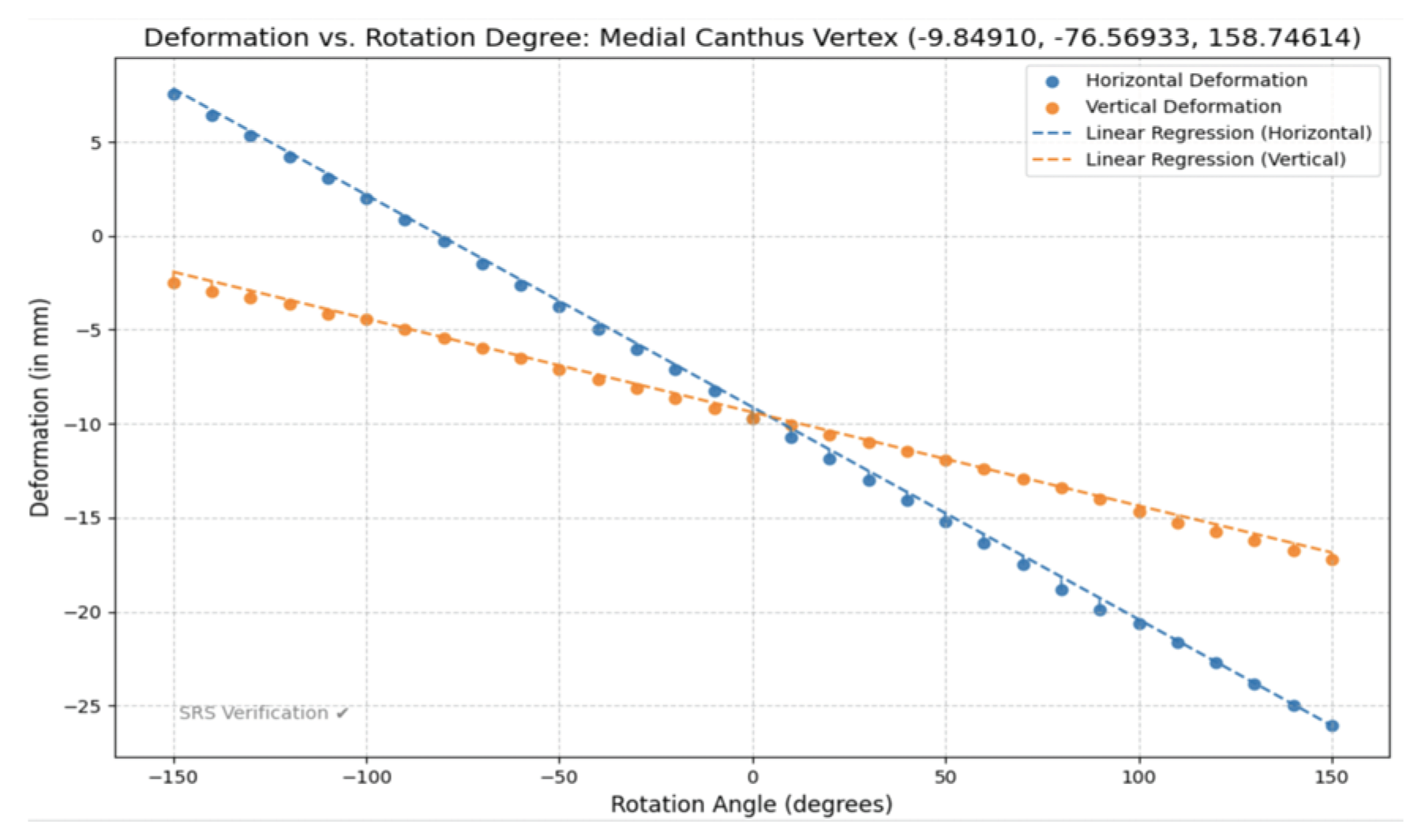
Modeling the Multivariate Linear Regression Trained Dataset [-150, 150] and Soccer-Ball Ocular Impact at the Medial Canthus Vertex (-9.84910, -76.56933, 158.74614).
Figure 16.
Modeling the Multivariate Linear Regression Trained Dataset [-150, 150] and Soccer-Ball Ocular Impact at the Medial Canthus Vertex (-9.84910, -76.56933, 158.74614).
Figure 17.
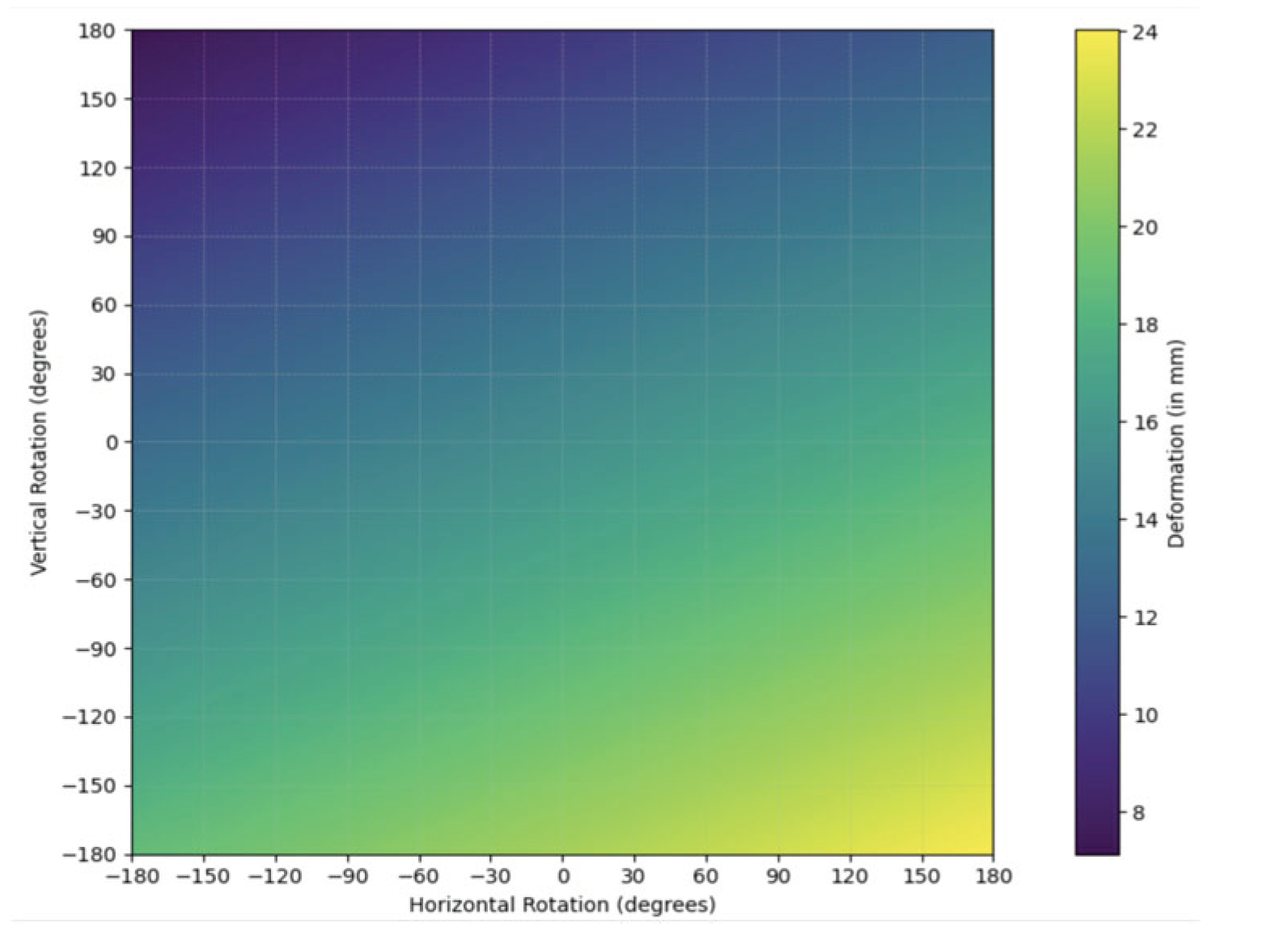
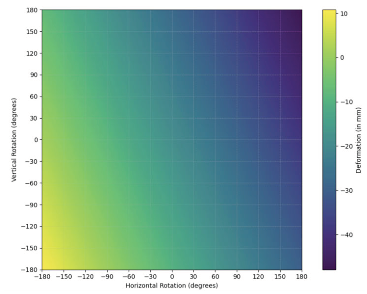
Modeling estimated deformation through multivariate linear regression equation and heat map analysis with step size 0.1 across range [-180, 180] generating 12,967,201 (3601 × 3601) data points for Medial Canthus Vertex (-9.84910, -76.56933, 158.74614).
Figure 17.
Modeling estimated deformation through multivariate linear regression equation and heat map analysis with step size 0.1 across range [-180, 180] generating 12,967,201 (3601 × 3601) data points for Medial Canthus Vertex (-9.84910, -76.56933, 158.74614).
Figure 18.
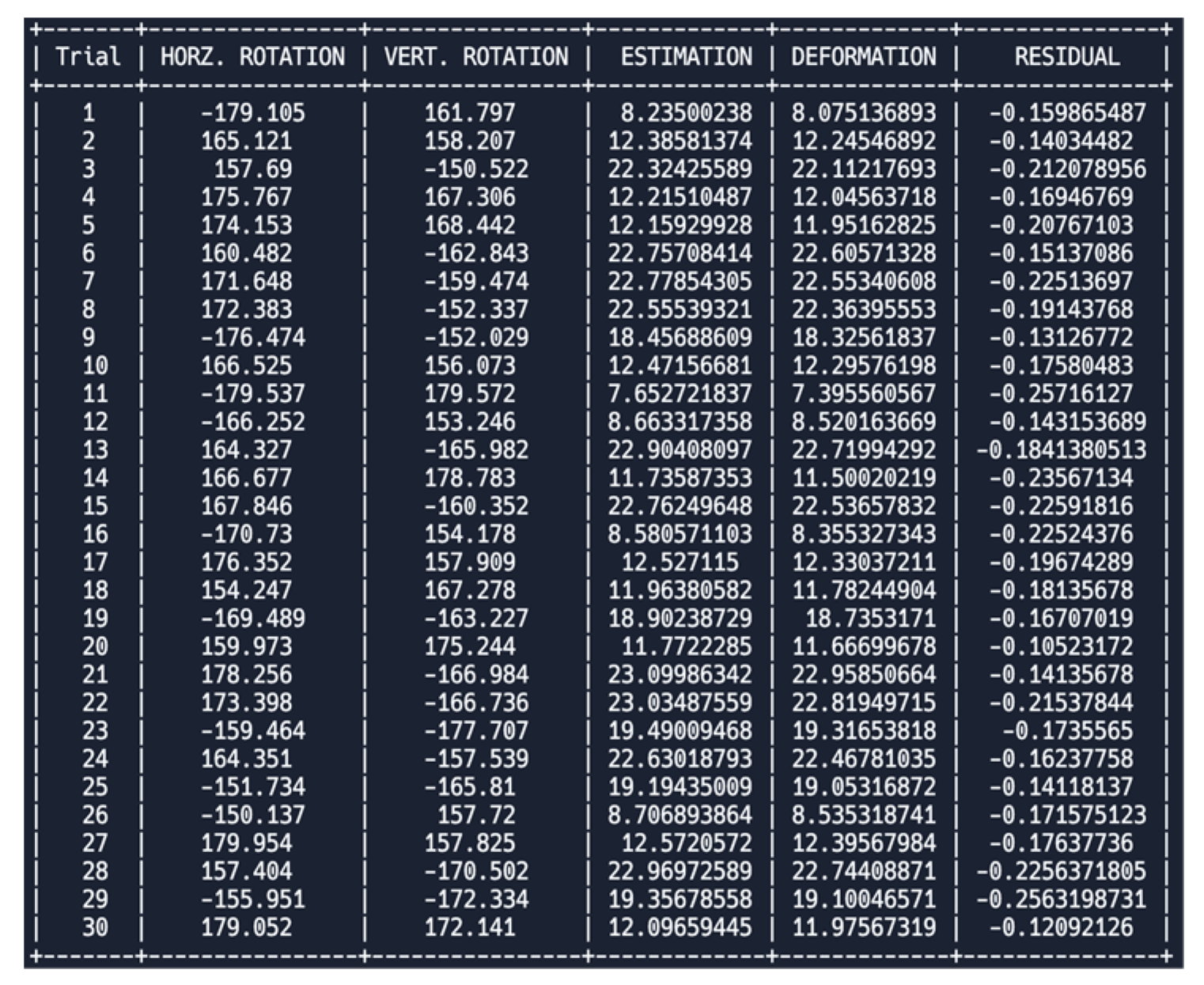
Modeling Simple Random Sample (SRS) data from thirty trials (n=30) to model-verify multivariate linear regression equation across [-180, 150] U [150, 180] rotating both horizontally and vertically at Medial Canthus Vertex (-9.84910, -76.56933, 158.74614).
Figure 18.
Modeling Simple Random Sample (SRS) data from thirty trials (n=30) to model-verify multivariate linear regression equation across [-180, 150] U [150, 180] rotating both horizontally and vertically at Medial Canthus Vertex (-9.84910, -76.56933, 158.74614).
Table 4.
Statistical Analyses and Equations for Soccer-Ball Ocular Impact at Various Angles at Medial Canthus Vertex (-9.84910, -76.56933, 158.74614). H represents horizontal and V represents vertical.
Table 4.
Statistical Analyses and Equations for Soccer-Ball Ocular Impact at Various Angles at Medial Canthus Vertex (-9.84910, -76.56933, 158.74614). H represents horizontal and V represents vertical.
| Modified Multivariate Linear Regression Equation |
(-9.11361016499-0.1129268636h) + (-9.38390463739-0.04976040045v) |
| Pearson’s Correlation Coefficient (R-value) |
H: (-0.999859123964855) & V: (-0.999461271533783) |
| Coefficient of Determination |
H: (0.999718267775767) & V: (0.998922833295926) |
| Adjusted Coefficient of Determination |
H: (0.999708552871483) & V: (0.998885689616475) |
| Modified Mean Absolute Error (MAE) |
H: (0.39914274652) & V: (0.38116878281) |
| P-value test for linearity |
H: (8.718e-06) & V: (8.770e-06) |
Figure 19.
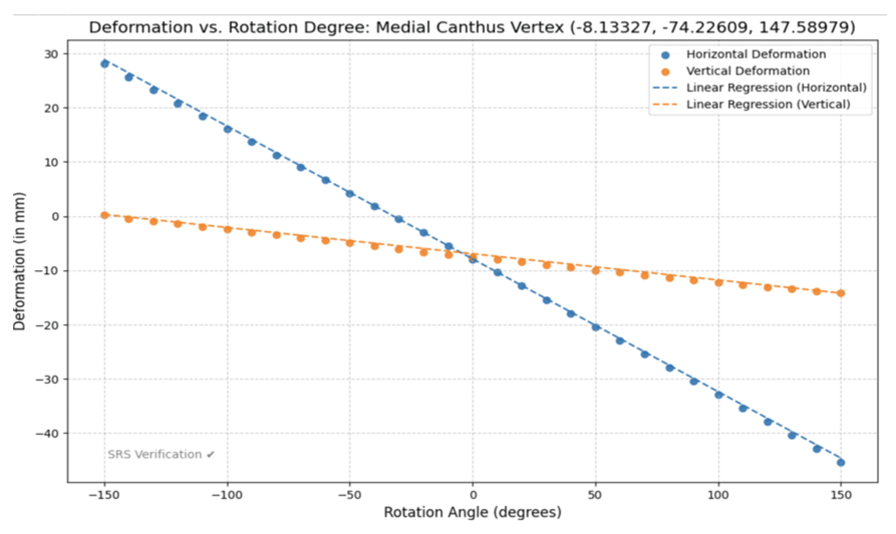
Modeling the Multivariate Linear Regression Trained Dataset [-150, 150] and Soccer-Ball Ocular Impact at the Medial Canthus Vertex (-8.13327, -74.22609, 147.58979).
Figure 19.
Modeling the Multivariate Linear Regression Trained Dataset [-150, 150] and Soccer-Ball Ocular Impact at the Medial Canthus Vertex (-8.13327, -74.22609, 147.58979).
Figure 20.
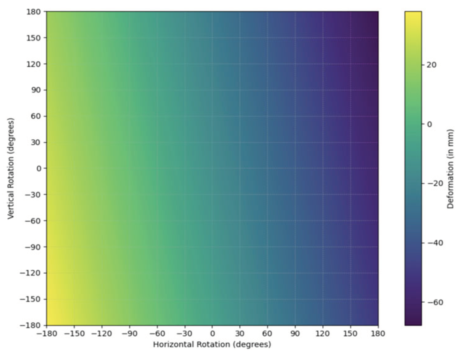
Modeling estimated deformation through multivariate linear regression equation and heat map analysis with step size 0.1 across range [-180, 180] generating 12,967,201 (3601 × 3601) data points for Medial Canthus Vertex (-8.13327, -74.22609, 147.58979).
Figure 20.
Modeling estimated deformation through multivariate linear regression equation and heat map analysis with step size 0.1 across range [-180, 180] generating 12,967,201 (3601 × 3601) data points for Medial Canthus Vertex (-8.13327, -74.22609, 147.58979).
Figure 21.
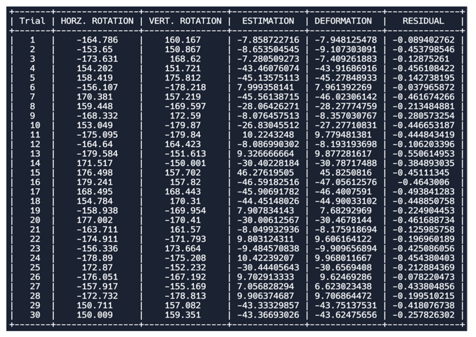
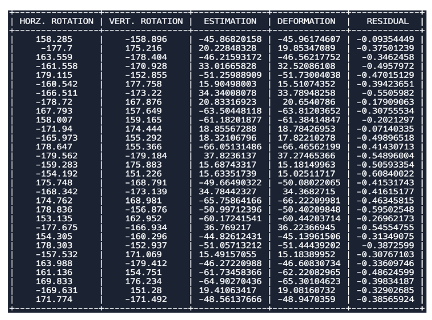
Modeling Simple Random Sample (SRS) data from thirty trials (n=30) to model-verify multivariate linear regression equation across [-180, 150] U [150, 180] rotating both horizontally and vertically at Medial Canthus Vertex (-8.13327, -74.22609, 147.58979).
Figure 21.
Modeling Simple Random Sample (SRS) data from thirty trials (n=30) to model-verify multivariate linear regression equation across [-180, 150] U [150, 180] rotating both horizontally and vertically at Medial Canthus Vertex (-8.13327, -74.22609, 147.58979).
Table 5.
Statistical Analyses and Equations for Soccer-Ball Ocular Impact at Various Angles at Medial Canthus Vertex (-8.13327, -74.22609, 147.58979). H represents horizontal and V represents vertical.
Table 5.
Statistical Analyses and Equations for Soccer-Ball Ocular Impact at Various Angles at Medial Canthus Vertex (-8.13327, -74.22609, 147.58979). H represents horizontal and V represents vertical.
| Modified Multivariate Linear Regression Equation |
(-7.87051397128-0.2448169116h) + (-6.93127629473-0.0483614033018307v) |
| Pearson’s Correlation Coefficient (R-value) |
H: (-0.999932712111716) & V: (-0.999240597399331) |
| Coefficient of Determination |
H: (0.999865428751092) & V: (0.998481771490971) |
| Adjusted Coefficient of Determination |
H: (0.999860788363198) & V: (0.998429418783763) |
| Modified Mean Absolute Error (MAE) |
H: (0.70908842064) & V: (0.53925224807) |
| P-value test for linearity |
H: (8.708e-06) & V: (8.799e-06) |
Figure 22.
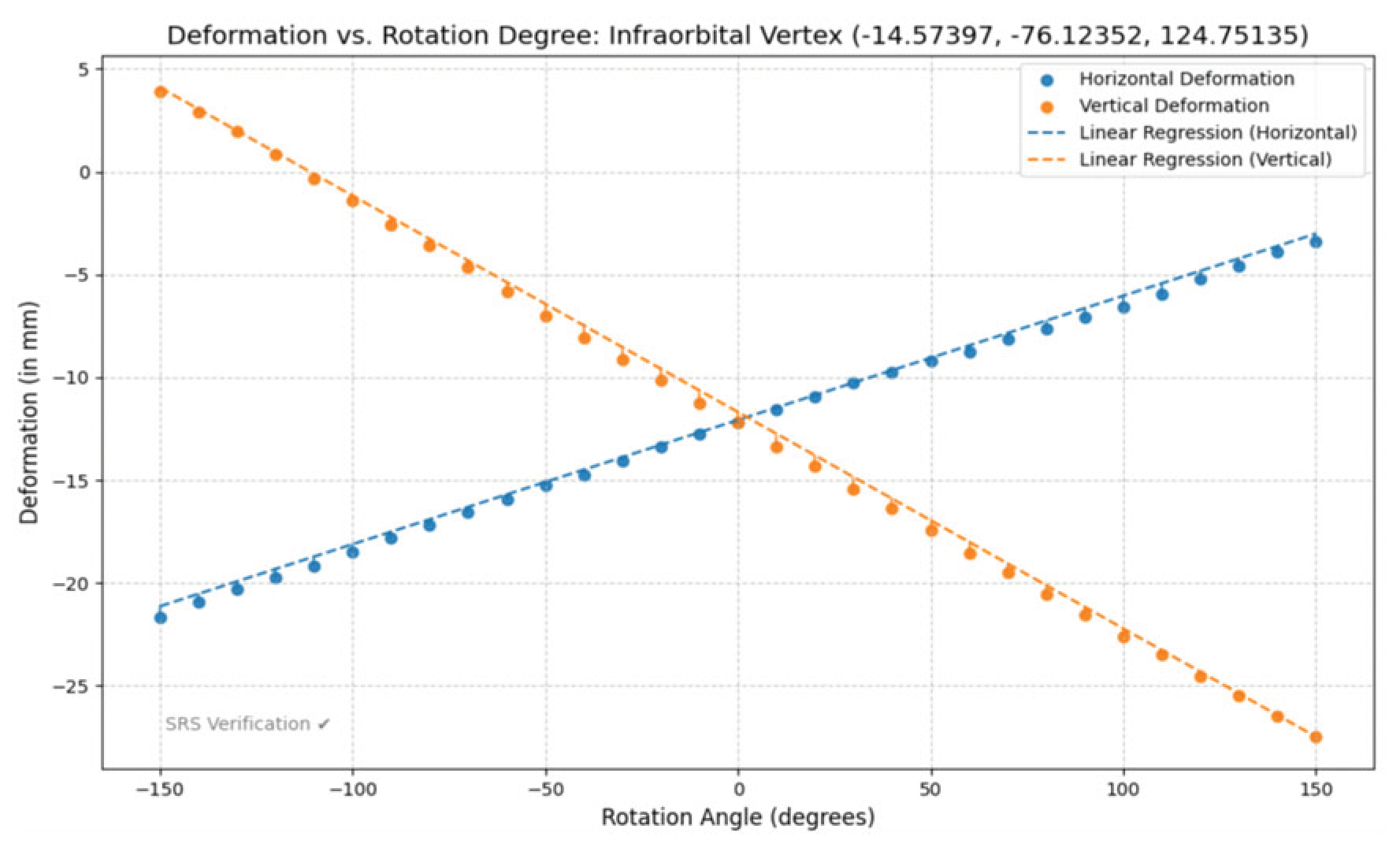
Modeling the Multivariate Linear Regression Trained Dataset [-150, 150] and Soccer-Ball Ocular Impact at the Infraorbital Vertex (-14.57397, -76.12352, 124.75135).
Figure 22.
Modeling the Multivariate Linear Regression Trained Dataset [-150, 150] and Soccer-Ball Ocular Impact at the Infraorbital Vertex (-14.57397, -76.12352, 124.75135).
Figure 23.
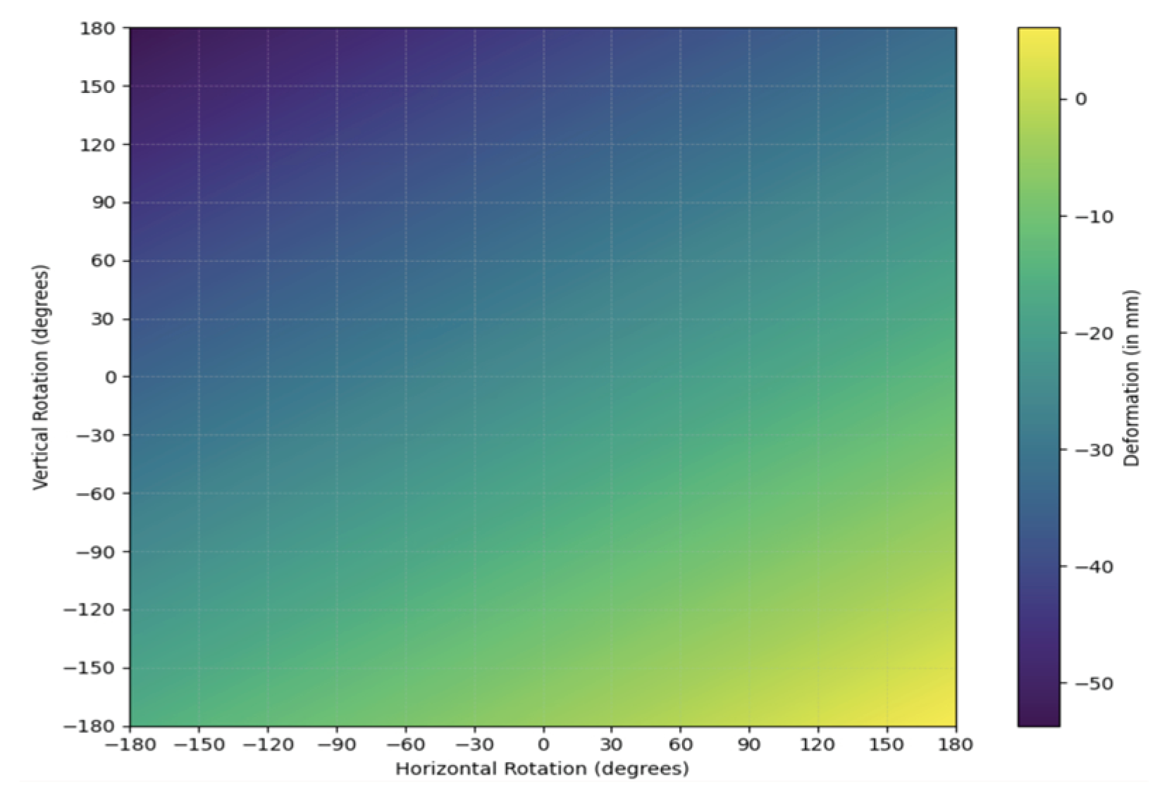
Modeling estimated deformation through multivariate linear regression equation and heat map analysis with step size 0.1 across range [-180, 180] generating 12,967,201 (3601 × 3601) data points for Infraorbital Vertex (-14.57397, -76.12352, 124.75135).
Figure 23.
Modeling estimated deformation through multivariate linear regression equation and heat map analysis with step size 0.1 across range [-180, 180] generating 12,967,201 (3601 × 3601) data points for Infraorbital Vertex (-14.57397, -76.12352, 124.75135).
Figure 24.
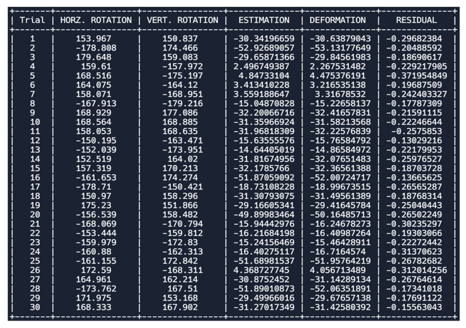
Modeling Simple Random Sample (SRS) data from thirty trials (n=30) to model-verify multivariate linear regression equation across [-180, 150] U [150, 180] rotating both horizontally and vertically at Infraorbital Vertex (-14.57397, -76.12352, 124.75135).
Figure 24.
Modeling Simple Random Sample (SRS) data from thirty trials (n=30) to model-verify multivariate linear regression equation across [-180, 150] U [150, 180] rotating both horizontally and vertically at Infraorbital Vertex (-14.57397, -76.12352, 124.75135).
Table 6.
Statistical Analyses and Equations for Soccer-Ball Ocular Impact at Various Angles at Infraorbital Vertex (-14.57397, -76.12352, 124.75135). H represents horizontal and V represents vertical.
Table 6.
Statistical Analyses and Equations for Soccer-Ball Ocular Impact at Various Angles at Infraorbital Vertex (-14.57397, -76.12352, 124.75135). H represents horizontal and V represents vertical.
| Modified Multivariate Linear Regression Equation |
(-12.0772487785+0.06039605328h) + (-11.6901967461-0.1052362498v) |
| Pearson’s Correlation Coefficient (R-value) |
H: (0.9996395114) & V: (-0.9997886199) |
| Coefficient of Determination |
H: (0.9904444789) & V: (0.9995772845) |
| Adjusted Coefficient of Determination |
H: (0.9992542959) & V: (0.9995627081) |
| Modified Mean Absolute Error (MAE) |
H: (0.4099082499) & V: (0.5495383813) |
| P-value test for linearity |
H: (8.746e-06) & V: (8.727e-06) |
Figure 25.
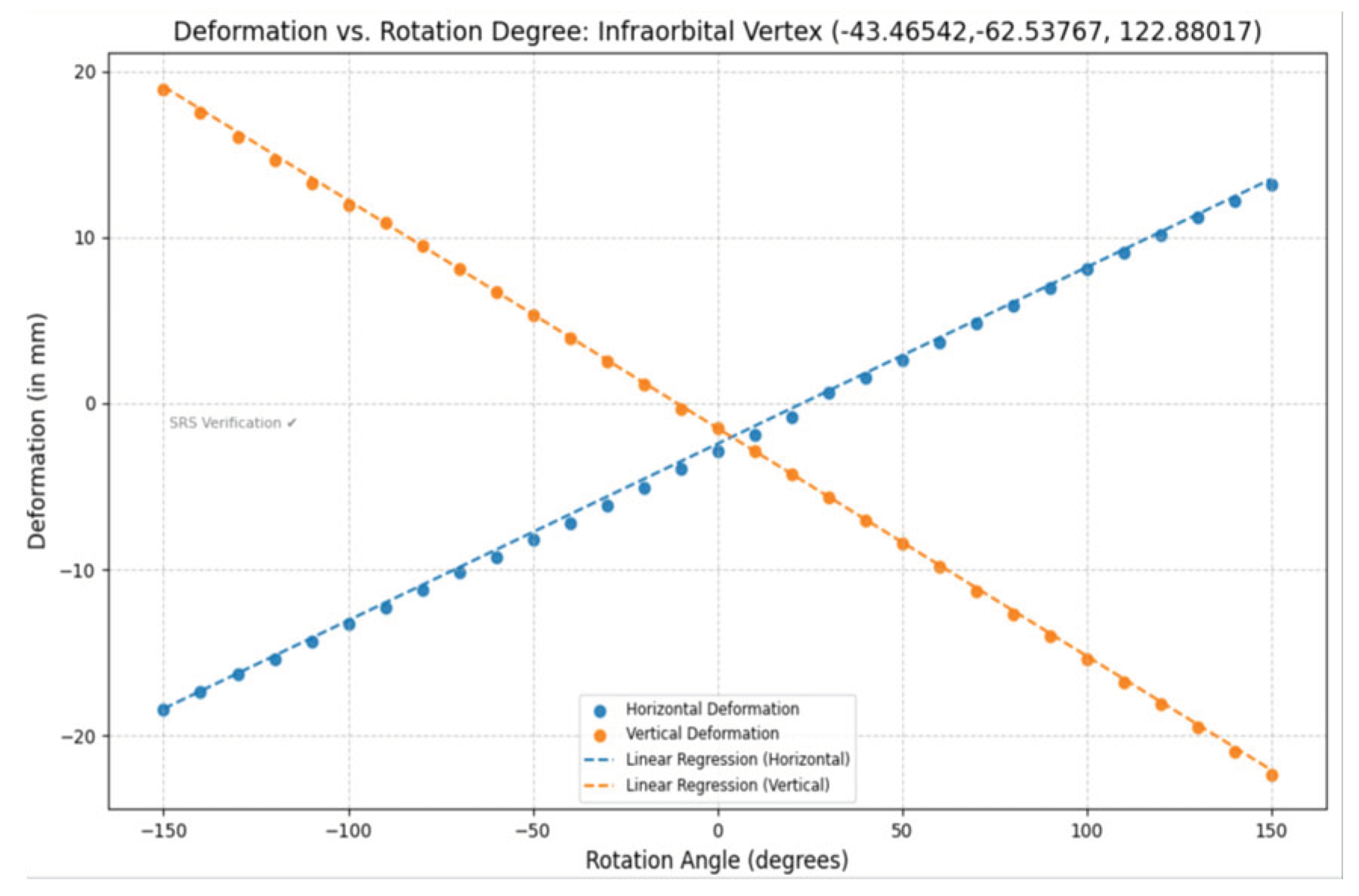
Modeling the Multivariate Linear Regression Trained Dataset [-150, 150] and Soccer-Ball Ocular Impact at the Infraorbital Vertex (-43.46542,-62.53767, 122.88017).
Figure 25.
Modeling the Multivariate Linear Regression Trained Dataset [-150, 150] and Soccer-Ball Ocular Impact at the Infraorbital Vertex (-43.46542,-62.53767, 122.88017).
Figure 26.
Modeling estimated deformation through multivariate linear regression equation and heat map analysis with step size 0.1 across range [-180, 180] generating 12,967,201 (3601 × 3601) data points for Infraorbital Vertex (-43.46542,-62.53767, 122.88017).
Figure 26.
Modeling estimated deformation through multivariate linear regression equation and heat map analysis with step size 0.1 across range [-180, 180] generating 12,967,201 (3601 × 3601) data points for Infraorbital Vertex (-43.46542,-62.53767, 122.88017).
Figure 27.
Modeling Simple Random Sample (SRS) data from thirty trials (n=30) to model-verify multivariate linear regression equation across [-180, 150] U [150, 180] rotating both horizontally and vertically at Infraorbital Vertex (-43.46542,-62.53767, 122.88017).
Figure 27.
Modeling Simple Random Sample (SRS) data from thirty trials (n=30) to model-verify multivariate linear regression equation across [-180, 150] U [150, 180] rotating both horizontally and vertically at Infraorbital Vertex (-43.46542,-62.53767, 122.88017).
Table 7.
Statistical Analyses and Equations for Soccer-Ball Ocular Impact at Various Angles at Infraorbital Vertex (-43.46542,-62.53767, 122.88017). H represents horizontal and V represents vertical.
Table 7.
Statistical Analyses and Equations for Soccer-Ball Ocular Impact at Various Angles at Infraorbital Vertex (-43.46542,-62.53767, 122.88017). H represents horizontal and V represents vertical.
| Modified Multivariate Linear Regression Equation |
(-12.0772487785+0.06039605328h) + (-11.6901967461-0.1052362498v) |
| Pearson’s Correlation Coefficient (R-value) |
H: (0.9996395114) & V: (-0.9997886199) |
| Coefficient of Determination |
H: (0.9904444789) & V: (0.9995772845) |
| Adjusted Coefficient of Determination |
H: (0.9992542959) & V: (0.9995627081) |
| Modified Mean Absolute Error (MAE) |
H: (0.4099082499) & V: (0.5495383813) |
| P-value test for linearity |
H: (8.746e-06) & V: (8.727e-06) |
Figure 28.
Modeling the Multivariate Linear Regression Trained Dataset [-150, 150] and Soccer-Ball Ocular Impact at the Lateral Canthus Vertex (-57.93342,-45.62785, 133.72293).
Figure 28.
Modeling the Multivariate Linear Regression Trained Dataset [-150, 150] and Soccer-Ball Ocular Impact at the Lateral Canthus Vertex (-57.93342,-45.62785, 133.72293).
Figure 29.
Modeling estimated deformation through multivariate linear regression equation and heat map analysis with step size 0.1 across range [-180, 180] generating 12,967,201 (3601 × 3601) data points for Lateral Canthus Vertex (-57.93342,-45.62785,133.72293)
Figure 29.
Modeling estimated deformation through multivariate linear regression equation and heat map analysis with step size 0.1 across range [-180, 180] generating 12,967,201 (3601 × 3601) data points for Lateral Canthus Vertex (-57.93342,-45.62785,133.72293)
Figure 30.
Modeling Simple Random Sample (SRS) data from thirty trials (n=30) to model-verify multivariate linear regression equation across [-180, 150] U [150, 180] rotating both horizontally and vertically at Lateral Canthus Vertex (-57.93342, -45.62785, 133.72293).
Figure 30.
Modeling Simple Random Sample (SRS) data from thirty trials (n=30) to model-verify multivariate linear regression equation across [-180, 150] U [150, 180] rotating both horizontally and vertically at Lateral Canthus Vertex (-57.93342, -45.62785, 133.72293).
Table 8.
Statistical Analyses and Equations for Soccer-Ball Ocular Impact at Various Angles at Lateral Canthus Vertex (-57.93342,-45.62785,133.72293). H represents horizontal and V represents vertical.
Table 8.
Statistical Analyses and Equations for Soccer-Ball Ocular Impact at Various Angles at Lateral Canthus Vertex (-57.93342,-45.62785,133.72293). H represents horizontal and V represents vertical.
| Modified Multivariate Linear Regression Equation |
(17.7033624616+0.135480098536461h) + (17.3687473544+0.470870533672953v) |
| Pearson’s Correlation Coefficient (R-value) |
H: (0.998139108703394) & V: (0.999980680897641) |
| Coefficient of Determination |
H: (0.996281680323205) & V: (0.999961362168509) |
| Adjusted Coefficient of Determination |
H: (0.996153462403315) & V: (0.999960029829492) |
| Modified Mean Absolute Error (MAE) |
H: (1.290896539) & V: (0.77177687766) |
| P-value test for linearity |
H: (8.945e-06) & V: (8.702e-06) |
Figure 31.
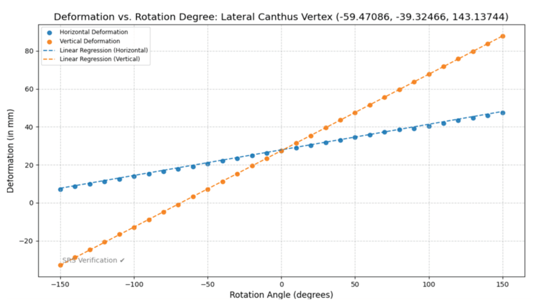
Modeling the Multivariate Linear Regression Trained Dataset [-150, 150] and Soccer-Ball Ocular Impact at the Lateral Canthus Vertex (-59.47086, -39.32466, 143.13744).
Figure 31.
Modeling the Multivariate Linear Regression Trained Dataset [-150, 150] and Soccer-Ball Ocular Impact at the Lateral Canthus Vertex (-59.47086, -39.32466, 143.13744).
Figure 32.
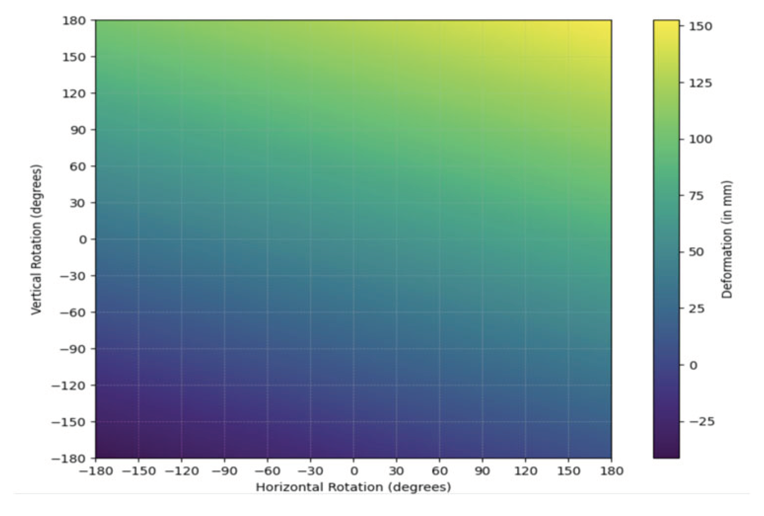
Modeling estimated deformation through multivariate linear regression equation and heat map analysis with step size 0.1 across range [-180, 180] generating 12,967,201 (3601 × 3601) data points for Lateral Canthus Vertex (-59.47086, -39.32466, 143.13744).
Figure 32.
Modeling estimated deformation through multivariate linear regression equation and heat map analysis with step size 0.1 across range [-180, 180] generating 12,967,201 (3601 × 3601) data points for Lateral Canthus Vertex (-59.47086, -39.32466, 143.13744).
Figure 33.
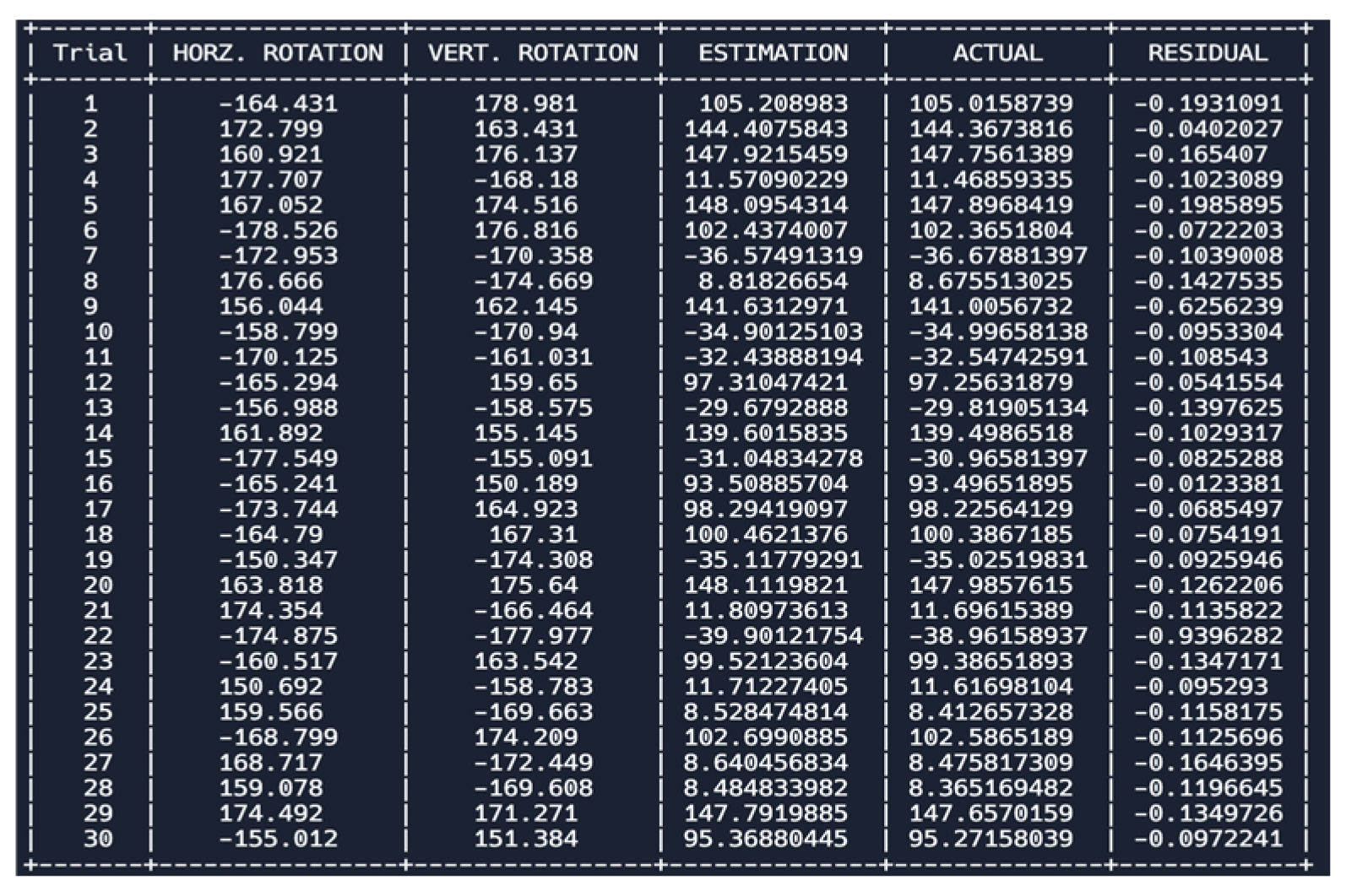
Modeling Simple Random Sample (SRS) data from thirty trials (n=30) to model-verify multivariate linear regression equation across [-180, 150] U [150, 180] rotating both horizontally and vertically at Lateral Canthus Vertex (-59.47086, -39.32466, 143.13744).
Figure 33.
Modeling Simple Random Sample (SRS) data from thirty trials (n=30) to model-verify multivariate linear regression equation across [-180, 150] U [150, 180] rotating both horizontally and vertically at Lateral Canthus Vertex (-59.47086, -39.32466, 143.13744).
Table 9.
Statistical Analyses and Equations for Soccer-Ball Ocular Impact at Various Angles at Lateral Canthus Vertex (-59.47086, -39.32466, 143.13744). H represents horizontal and V represents vertical.
Table 9.
Statistical Analyses and Equations for Soccer-Ball Ocular Impact at Various Angles at Lateral Canthus Vertex (-59.47086, -39.32466, 143.13744). H represents horizontal and V represents vertical.
| Modified Multivariate Linear Regression Equation |
(27.8761266653+0.134800111934311h) + (27.77869596+0.402574947727541v) |
| Pearson’s Correlation Coefficient (R-value) |
H: (0.999785431318762) & V: (0.999992629717107) |
| Coefficient of Determination |
H: (0.999570908677243) & V: (0.999985259488535) |
| Adjusted Coefficient of Determination |
H: (0.999556112424734) & V: (0.999984751195036) |
| Modified Mean Absolute Error (MAE) |
H: (0.29394282419) & V: (0.77177687766) |
| P-value test for linearity |
H: (8.727e-06) & V: (8.700e-06) |
Figure 34.
Hertzian Contact Stress Equation modeling at the supraorbital region to determine thickness of the apparatus. *Considering a professional regulation size 5 soccer ball and a ball inflation pressure of 1.10 bar (16 psi), there is an average peak impact force of 3606 N. A FIFA size five’s ball has a radius of 220mm.
Figure 35.
Hertzian Contact Stress Equation modeling at the lateral canthus region to determine thickness of the apparatus. *Considering a professional regulation size 5 soccer ball and a ball inflation pressure of 1.10 bar (16 psi), there is an average peak impact force of 3606 N. A FIFA size five’s ball has a radius of 220mm.
Figure 36.
Hertzian Contact Stress Equation modeling at the medial canthus region to determine thickness of the apparatus. *Considering a professional regulation size 5 soccer ball and a ball inflation pressure of 1.10 bar (16 psi), there is an average peak impact force of 3606 N. A FIFA size five’s ball has a radius of 220mm.
Figure 37.
Hertzian Contact Stress Equation modeling at the infraorbital region to determine thickness of the apparatus. *Considering a professional regulation size 5 soccer ball and a ball inflation pressure of 1.10 bar (16 psi), there is an average peak impact force of 3606 N. A FIFA size five’s ball has a radius of 220mm.


