1. Introduction
Methane is an attractive option for the new generation of thrust chambers [
1,
2]. This fuel has promising capabilities due to its high specific impulse, easy production and handling [
3]. However, several challenges related to ignition, mixing, combustion stability, and safe operation demand further research [
4,
5]. The design process of modern rocket engines relies on Computational Fluid Dynamics (CFD) to address these issues. Numerical simulations are a fast and inexpensive tool to investigate design modifications and optimize geometrical features. In addition, they can facilitate the understanding of test results since every relevant physical field is accessible. Consequently, CFD is an integral part of the design process of combustion chambers [
6,
7,
8,
9]. Traditionally, Reynolds Averaged Navier-Stokes (RANS) solvers have been extensively used in industry due to their low computational cost. In methane thrust chambers, multiple researchers have used this methodology for both the combustion chamber [
10,
11,
12] and the cooling system [
13,
14,
15,
16,
17]. The most relevant handicap of this approach is the suppression of transient behavior, which excessively restricts the degrees of freedom of the turbulent flow dynamics. Important features and physical processes are subsequently canceled, reducing the simulation fidelity. This oversimplification is particularly relevant in combustion chambers of rocket engines. In such a scenario, classical assumptions of turbulence are challenged due to the extreme conditions that take place. Turbulent diffusion flames for space propulsion applications may exhibit exotic phenomena such as reversed energy transfer [
18], high anisotropy far from walls [
19], and flame-generated turbulence [
20,
21,
22,
23]. Conventional RANS models are unfit to capture these processes due to their inherent steady nature. Scale-resolving methods are a promising alternative to approach the complexity of turbulent combustion in liquid rocket engines. With growing computational resources, the applicability window for Large Eddy Simulations (LES) has experienced a significant widening over the last years [
24,
25,
26]. Despite their higher computational cost, this method circumvents most of the shortcomings associated with RANS by resolving the largest vortical structures. Under the current technological constraints, LES is the most accurate method in which the simulation of full-scale systems remains feasible [
27] (although at a high computational cost). Due to its potential, LES for combustion applications has awakened considerable interest in the last few years.
The application of LES requires modeling unresolved turbulent quantities at a subgrid level. The extended approaches have been validated using empirical results or higher-fidelity Direct Numerical Simulations (DNS). However, the conditions for which most models were devised differ from the extreme environment found in combustion chambers of liquid rocket engines. In such applications, chemical scales are very thin and fast due to the high pressures and the usage of pure oxygen as oxidizer. These conditions have dramatic repercussions on the computational cost, which is driven by the necessary flame front resolution [
28,
29]. Artificially Thickened Flame (ATF) models [
30,
31] are a powerful alternative to address this challenge. In this approach, diffusivity and reaction rates are artificially varied to thicken the flame front while preserving flame speed. This method can provide invaluable computational cost savings enabling coarser grids. ATF has been applied to a wide variety of configurations, including non-premixed combustion [
31], and particularly space propulsion engines [
32]. A thickened flame alters the overlapping between vortical and chemical scales, altering the original interactions between turbulence and chemistry.When a flame is artificially thickened, the Damköhler and other dimensionless numbers are altered with respect to the original configuration. Such modifications have the potential of falsifying fundamental interaction such as the sensitivity of the flame displacement speed to stretching. These changes have a profound impact in the overall feedback between turbulence and combustion and can imparity the validity of the simulation if they are not carefully addressed. Efficiency functions are common solution used to mitigate the effect of neglected physical features [
30,
33,
34]. Nonetheless, the performance and reliability of these models remains an unsolved challenge, which has motivated intensive research activity during the last years [
35,
36,
37]. Other remarkable approaches for LES modeling in turbulent combustion applications include the G-equation model [
38,
39] and the Flame Surface Density (FSD) models [
40].
The present paper focuses on the application of gradient models for closure of subgrid turbulent fluxes. This approach originates from the works of Clark et Al. [
41] and Vreman et al. [
42], which was later applied to combustion by Pierce and Moin [
43]. Gradient models can determine subgrid turbulent fluxes assuming their similarity with the projection of the involved variables in the filtered space. This approach is particularly attractive if the flame dynamics are the dominating physical process at the filter level. Such a scenario is particularly interesting in high-pressure combustion applications, where the flame is very thin, and the unresolved eddies have low energy. In such situations, the influence of chemical processes to fluid dynamics is the main unresolved effect at a subgrid scale. Modeling of these processes without resorting to ATF allows for a partial resolution of the flame front, preserving the original physical flow properties and relevant dimensionless numbers (e.g.
, and
). The present work evaluates the applicability of this approach for turbulent flames in conditions representative of rocket combustors. The performance and the behavior of the model coefficients are assessed with databases obtained from high-fidelity numerical simulations. In addition, an adaptive strategy based on the local burning conditions is proposed to enhance the model's performance.
The rest of the paper is structured as follows. A brief theoretical introduction to LES and turbulent diffusion flames is provided in Section II. The methodology used to retrieve the subgrid turbulent dynamics is discussed in Section III, where the performed numerical simulations are detailed. The gradient model enhancement for subgrid turbulent fluxes is introduced and validated in
Section 4. Finally, the results are summarized in
Section 5.
2. Theoretical Background
The present section discusses basic concepts involving Large Eddy Simulations in diffusion flames. First, the mathematical foundations for the notion of LES filters are introduced. Secondly, the conservation equations of reacting flow subject to filtering are briefly commented on, emphasizing the role of unresolved subgrid fluxes and existing models. Finally, the most relevant characterization parameters in turbulent non-premixed combustion are presented to facilitate the discussion of the results.
2.1. Filters
In LES, the grid size
is sufficiently small to resolve large eddies appropriately, but the smallest ones (i.e., the Kolmogorov eddies
)are insufficiently resolved, as
[
44]. Therefore, unlike in DNS, it is not possible to assume a laminar behavior at subgrid levels, and statistical mechanics are relevant at these scales. The process of resolving a turbulent flow using a coarser resolution than necessary can be seen as applying a low-pass filter. In general, the application of a filter
on a quantity
can be defined as:
In variable-density flows, it is more convenient to perform the spatial integration weighing for density, as suggested by Favre [
45]. This operation can be expressed as:
Which is denoted as the Favre-filtered value of
. There is a wide variety of filters that can be applied [
28,
46,
47]. In the frame of the present work, top-hat filters have been used because of their simplicity. These mathematical operators are explicitly defined as:
where
are the spatial coordinates of the considered location. This filter corresponds to the average over a cubic box centered at
. In the frame of LES solvers, cut-off and Gaussian filters are other common alternative filtering options, but they are not detailed in this text for the sake of brevity.
2.2. Filtered Conservation Equations and Modeling
The presented filters can be applied to the transient conservation equations of a turbulent reacting flow to obtain a filtered LES version, which is formally very similar to their RANS counterparts [
28]:
Conservation of momentum:
Conservation of chemical species:
where
and
denote the mass fraction and the chemical production rate of the
chemical species. In addition,
represents the
component of the diffusion velocity
for the
chemical species.
In this equation,
denotes the thermal conductivity, and
the enthalpy change rate due to chemical reactions. Several terms in the presented equations are unresolved and require modeling. The present work focuses on the subgrid turbulent fluxes, which have the general form
. The most relevant ones are the subgrid stresses, which constitute the main unresolved term in the conservation of momentum equation:
This element is the only term requiring modeling in constant-density non-reactive flows. Therefore, it plays a key role in any application, and it has been the subject of intense research during the last decades. Smagorinsky [
48] pioneered a closure strategy based on the Boussinesq approximation:
where
denotes the filtered strain rate tensor, and
is a model constant, originally assumed to be universal. The application of this model requires the a priori knowledge of
, which can be extracted from experimental data or DNS. This motivated the research of this value under different setups [
49,
50,
51]. These studies revealed a good overall model performance, but the optimized constant
varied by a factor of 2 between different experiments. In addition, this constant has been observed to be sensitive to the used filter width
[
52,
53]. To circumvent these challenges, Germano and Lilly proposed a dynamic approach in which
was no longer a constant but a dynamically adaptable coefficient. The actual value is then determined from the problem resolution at a test level with larger filter widths
. This strategy has proved excellent performance in various applications [
54]. In compressible turbulence, modeling the diagonal part of the subgrid stresses i.e.
is required as well. For low Mach number flows, the diagonal component is usually absorbed into the filtered pressure field
Yoshizawa [
55] proposed a model for the trace of the subgrid Reynolds stresses formally similar to Smagorinky's approach. However, the influence of this term is very limited, and its relevance is primarily restricted to highly compressible flows [
56].
In reacting flows, the subgrid fluxes of chemical species (i.e.
) are unresolved as well. These scalars are usually modeled resorting to the gradient assumption [
28], which requires determining the subgrid turbulent viscosity and Schmidt number. These values are commonly retrieved using strategies analogous to the Smagorinski formulation, and assuming constant turbulent Schmidt number. The subgrid heat flux (i.e.
) is a relevant unresolved term within the energy conservation equation (7). A popular approach suggested by Eidson [
57] models this term assuming proportionality between the energy transfer from resolved to subgrid levels and the filtered temperature gradient
.
The introduced models were mainly conceived for incompressible non-reactive flows with low Damköhler numbers. Nonetheless, in high-pressure combustion applications, where the flame dynamics are very fast, strong interactions between turbulence and combustion may appear at a subgrid level. This circumstance can limit the validity of extended subgrid models due to the onset of unforeseen interactions. For example, the Boussinesq approximation prevents capturing reversed turbulent kinetic energy transfer, which is known to be relevant in turbulent combustion [
18,
58]. In addition, turbulent flames can display spectacular anisotropic features, even at the smallest vortical scales. Therefore, the combustion community has dedicated a significant effort in developing models able to cope with the challenges inherent to reacting flows.
Clark et. al [
41] and Vreman et. al [
42] derived gradient-based models which allow to express the subgrid stresses using the following similarity law:
This idea was further exploited by Pierce and Moin [
43], who combined it with the notion of scale-similarity [
59] to deduce the following general expression for subgrid covariances:
Models following this expression have been successfully used in turbulent combustion LES to determine relevant unresolved statistics, such as the subgrid variance of the turbulent mixture fraction
[
43,
60,
61] or the subgrid scalar dissipation rate
[
61,
62].
2.3. Turbulent Diffusion Flames
In turbulent diffusion flames, the propellants are injected separately and rely on turbulent and molecular diffusion to mix and burn. A comprehensive analysis of these physical systems poses a formidable challenge exceeding the scope of the present work. The reader is advised to review the available literature [
63,
64] for a detailed overview of turbulent non-premixed combustion. In this section, only the most relevant indicators to describe non-premixed flames are introduced due to their relevance in the model discussion.
2.3.1. Flame Index FI
Real combustion applications are neither purely premixed nor non-premixed. Instead, there is usually a coexistence between these two conditions. The flame index definition proposed by Yamashita et al. [
65] aims to evaluate the local regime at which combustion takes place:
where
represents the mass fraction, and the subscripts
and
stand for fuel and oxidizer, respectively. If combustion occurs in premixed conditions, both reactants are depleted simultaneously, and their gradients are aligned, yielding
. The opposite happens if combustion is locally non-premixed, with the gradients of fuel and oxidizer being opposed. In such a case, the flame index tends to
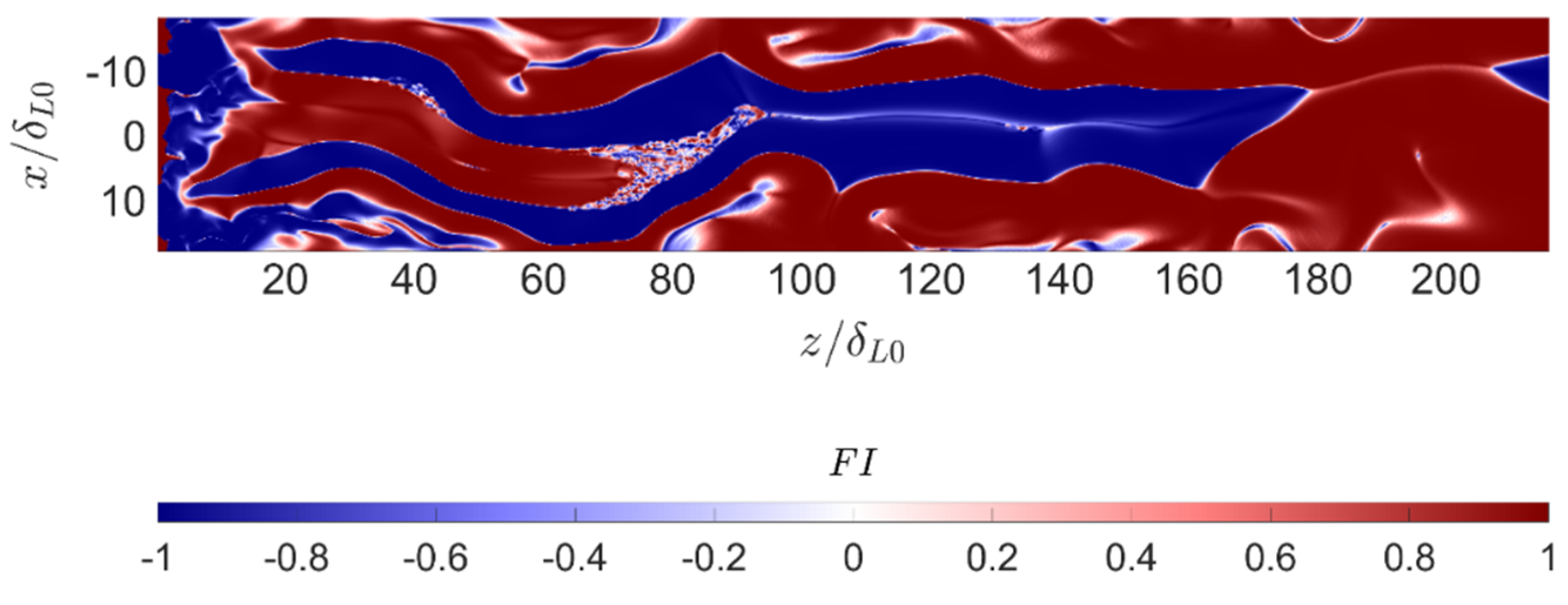
. An example of the instantaneous flame index is provided in
Figure 1. As can be seen, this parameter presents an almost binary distribution. This observation is in agreement with the trends found in one recent study [
66]. The pattern near injection displayed in
Figure 1 corresponds to the typical triple-flame structure [
67], with a non-premixed branch surrounded by one lean premixed branch and one fuel-rich premixed branch.
2.3.2. Mixture Fraction
In a turbulent diffusion flame, the mixture composition continuously fluctuates in space and time due to the competition between the injection boundary conditions and turbulent diffusion processes. The mixture fraction
is a conserved scalar characterizing the mixing state. This parameter essentially represents the local proportion of fuel coming from the fuel stream with respect to the total flow. In the frame of hydrocarbon combustion, the mixture fraction of the
chemical species, with
,
, and
carbon, hydrogen, and oxygen atoms can be expressed as:
where
and
denote the atomic weights of carbon, hydrogen, and oxygen, respectively. The individual mixture fractions can be combined to obtain the global value:
where
is the mass fraction of the
chemical species. Obviously, this parameter tends to unity towards the fuel and to zero close to the oxidizer injection. For methane–oxygen combustion, the stoichiometric oxidizer-to-fuel ratio is
, with a corresponding stoichiometric mixture fraction
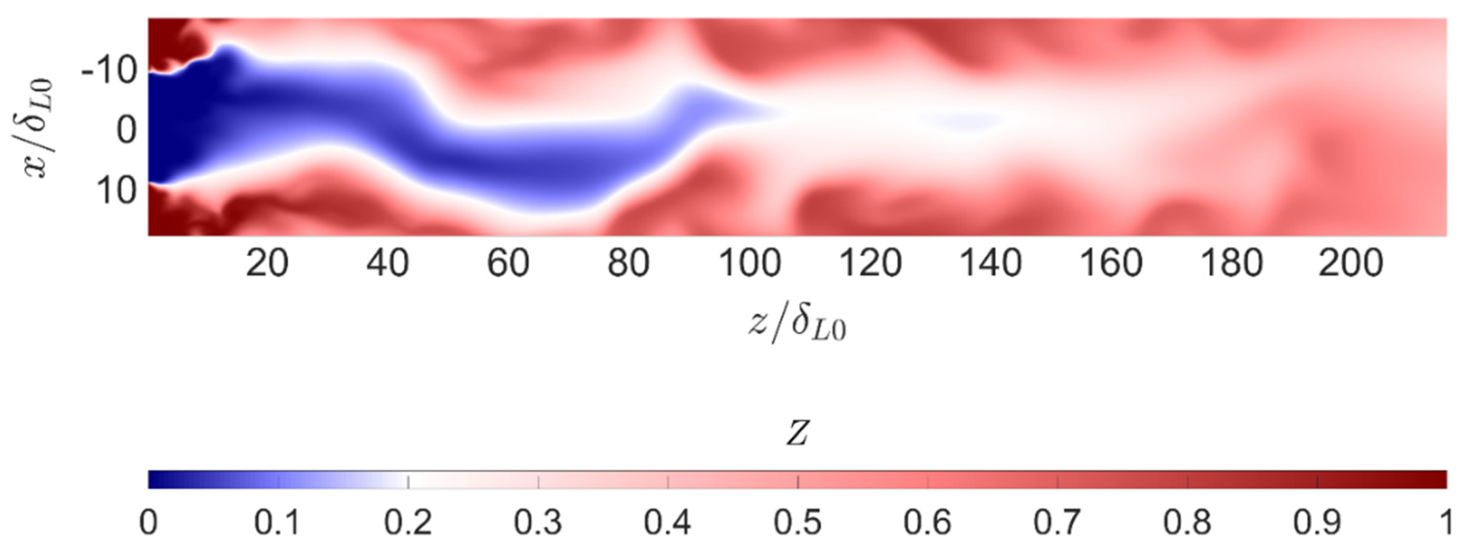
. An example of the instantaneous mixture fraction can be observed in
Figure 2. In this graphic, oxygen is injected at the center-left and methane at the top and bottom. The overall configuration is fuel-rich (
), this can be verified by observing the composition at downstream conditions, where the flow is well mixed, and the mixture fraction ranges from stoichiometric to mildly fuel-rich.
In the case of infinitely fast chemistry, combustion progress is strictly limited by the mixing configuration, which can be characterized by the mixture fraction and its dissipation rate
, representing the mixing intensity. If chemistry is very fast compared to turbulence, the flame dynamics can be decoupled from vortical interactions. In such cases, it is possible to solve the chemical problem independently and use tabulated results. This is the main assumption in the flamelet approach [
68], which allows for representing all chemistry with the single scalar
. The capability of the mixture fraction to solely describe the mixing state illustrates the relevance of this parameter.
2.3.3. Progress Variable
The progress variable
represents the degree of combustion process completion. It ranges from zero to unity, corresponding to reactants, and products, respectively. In diffusion flames, it is often described using an expression of the following sort, as proposed by Bray et al. [
69]:
where
is the reaction progress variable [
63,
70], and
is the equilibrium value at a specific given mixture fraction. The definition of a suitable function for the reaction progress variable is strongly dependent on the used propellant combination and the operating conditions. For oxygen–methane combustion at high pressures, the following expression has been used in previous research [
71,
72]:
where
denotes the molecular weight of the
species. This definition is based on the formulation proposed by Pierce and Moin [
73], which was applied in recent works [
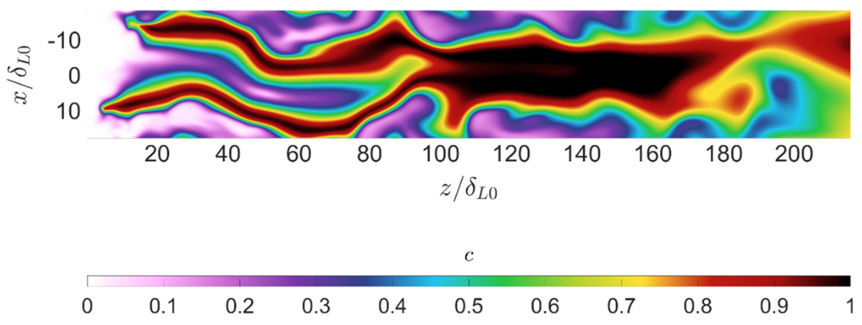
66] with similar setups as the current paper. Several variations have been incorporated to derive the expression in (16). The motivation behind these modifications was to account for specific chemical phenomena that take place in high-pressure combustion for space propulsion applications. An example of the instantaneous progress variable is displayed in
Figure 3. This instantaneous 2D cross-section cut corresponds to the same instant as those in
Figure 1 and
Figure 2. Near injection, the progress variable reaches unity at the stoichiometric line, where combustion occurs in a non-premixed regime. At downstream positions, the flow is more homogeneous, and combustion primarily develops in fuel-rich premixed conditions. These figures illustrate the complexity and spatial variability of a real turbulent diffusion flame.
3. Simulation Setup
Direct numerical simulations of a methane-oxygen turbulent non-premixed flame at 20 bar were conducted to generate a database for subgrid turbulence dynamics investigation. The present section describes the simulation framework and the strategy followed to filter the resolved fields. The results of the described simulations are used to investigate the subgrid scale dynamics in the following sections.
3.1. Strategy
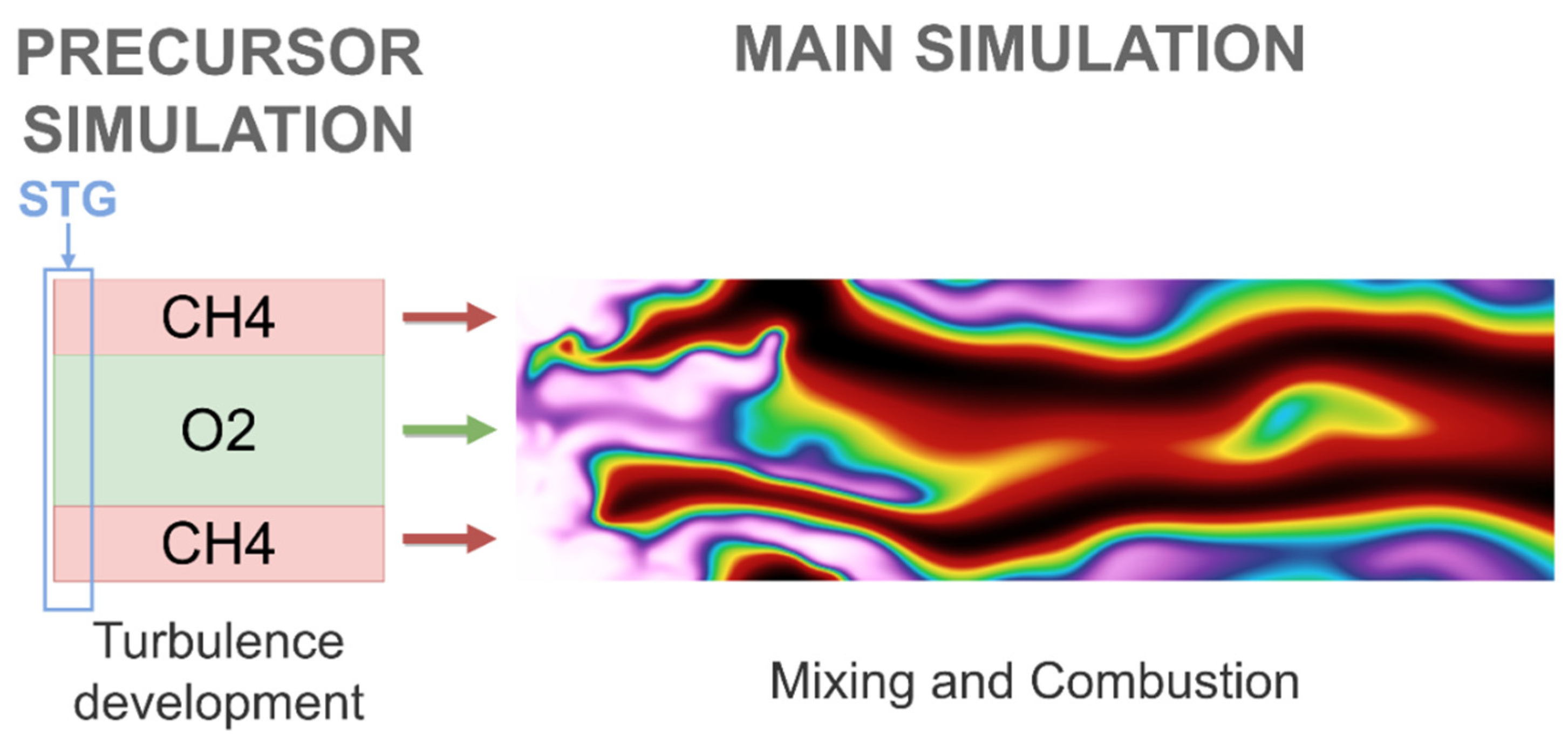
Two simulations are necessary to obtain the aimed turbulent diffusion flame. First, a precursor simulation is conducted to obtain realistic turbulent inlet boundary conditions. These fields are patched as the inlet boundary condition for the main simulation, where turbulent mixing and combustion take place. This second simulation is the one relevant within the scope of the present work. The overall scheme can be visualized in
Figure 4. The described database has been used in previous research [
74], where the reader can find a more detailed explanation concerning the simulation setup. This text is limited to a brief description for the sake of conciseness.
In the precursor simulation, periodic Synthetic Turbulence Generation (STG) takes place at the inlet, with the methodology discussed in [
75]. This approach is a modification of the periodic STG proposed by Morschbach et al. [
76], which is based on the work of Shur et al. [
77]. These methods derive from the original formulation developed by Kraichnan [
78], based on the superposition of several harmonics derived from a reference turbulent kinetic energy spectrum to generate synthetic turbulence. The STG development into realistic turbulence can be validated by examining classical statistics of turbulent flows such as higher-order derivatives and structure functions as proved in a previous work [
75]. The turbulent characteristics were selected considering the results of previous RANS simulations of a scale methane rocket combustor [
15]. It should be mentioned that the combustion pressure and the large eddy scales are roughly an order of magnitude smaller than what would be expected in real applications. These deviations are primarily motivated by the computational cost. Nonetheless, the chosen conditions are closer to realistic rocket combustion than what is usually found in the scientific literature. A summary of the turbulent characteristics at injection is provided in
Table 1.
The main simulation aims at recreating mixing and combustion nearby injection and far away from the combustion chamber walls. A stationary diffusion flame is simulated in a cuboid domain with dimensions 0.2 x 0.2 x 1.2 mm and resolved with 192 x 192 x 1152 cubic cells with constant geometry. This configuration corresponds to a grid spacing
. This cell size ensures enough resolution for the smallest Kolmogorov eddies [
44]. The used resolution was proved to ensure convergence of the turbulent statistics in a mesh sensitivity analysis virtually identical setups [
72,
79]. This grid size provides a resolution of the stoichiometric premixed flame front with roughly 5.3 cells. Nevertheless, in turbulent methane-oxygen diffusion flames the thinnest realized flamelets at least double this value, as evaluated in previous works [
72,
80]. Therefore, the effective flame front resolution is in the order of 10-20 cells. A resolution with a finer grid size (
and 384 x 384 x 2304 cells) was conducted to perform a mesh sensitivity analysis on the results, with marginal differences found as presented in section 4.2.1.
The transient reactive turbulent flow In the main simulation is computed using the reactive solver EBI-DNS [
81,
82,
83,
84]. This code package is embedded in the open-source software OpenFOAM [
85,
86] and was developed by the Engler-Bunte Institute (EBI) for combustion technology. EBI-DNS solves the unsteady compressible conservation equations using the Finite Volume Method (FVM) [
87,
88]. The capabilities of this software have been established in a large number of research works conducted during the last years [
89,
90,
91,
92,
93]. In a recent work [
94], Zirwes et al. validated the EBI-DNS code comparing its accuracy with state-of-the art explicit reactive solvers in a benchmark case of hydrogen flames interacting with Taylor-Green vortices. Cantera [
95] is used to compute detailed chemistry and transport properties. This code implements the mixture-averaged transport model as described by Kee
et al. [
96]. The diffusive mass flux is determined with the mixture-average model derived from the Maxwell-Stefan equations [
96]. Pressure and temperature diffusion (i.e. Soret effect) are neglected. The methane oxidation process is calculated with the finite rate method using a complex chemical mechanism developed by Slavinskaya
et al. [
97]. This reaction scheme was conceived for space propulsion applications at high pressures, and it has been extensively used in several numerical research in this field [
10,
98]. The relevant combustion parameters are displayed in
Table 2. Numerical diffusion is a major concern in unsteady numerical simulations, especially if implicit schemes are used. Zirwes et. al [
93] demonstrated that the used solver exhibits negligible numerical diffusion with a second order spatial discretization scheme and low CFL numbers. A mesh sensitivity analysis in an almost identical setup [
72] further supports the low risk of numerical diffusion polluting the solve’'s fidelity. In this previous work, marginal changes in averaged first and second order statistics were found for finer and coarser meshes. Since numerical diffusion is strongly dependent on the grid size, it is highly improbable that it plays a relevant role in the present context. The virtually identical results obtained with the finer grid size further support the low risk of numerical diffusion.
3.2. Filtering
The fully resolved results can be filtered using different filter widths
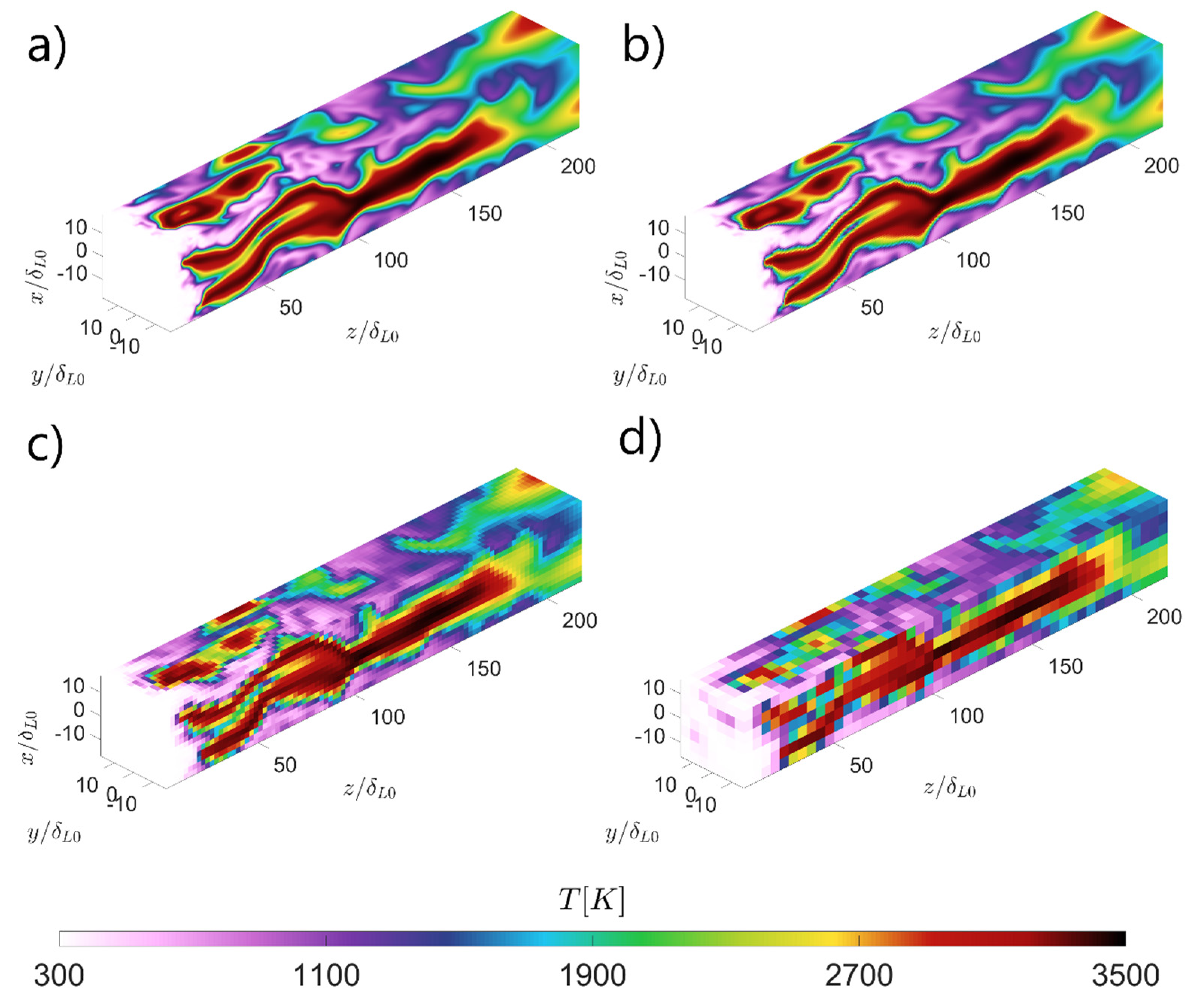
to obtain validation data subgrid models. This enables the measurement of the actual subgrid turbulent quantities. An output example for the filtering process can be visualized in
Figure 5, where the filtered temperature field with different widths
can be compared against the entirely resolved direct numerical simulation. A summary of the used filters is provided in
Table 2. As can be seen, large filter widths over DNS fields produces an excessive pixelation. Such results are physically unrealistic and cannot be the outcome of a numerically sound LES. However, if a top-hat filter with an excessive width is applied over a well resolved field, such unnatural results are feasible. The inaccuracy of such filter widths will be further commented on in the results section.
Figure 5.
Examples of different filtering widths: Direct numerical simulation (a), Filter width (b), Filter width (c), Filter width (d).
Figure 5.
Examples of different filtering widths: Direct numerical simulation (a), Filter width (b), Filter width (c), Filter width (d).
Table 3.
Summary of the used filters.
Table 3.
Summary of the used filters.
| Simulation |
Number of cells [x y z] |
] |
] |
|
192 x 192 x 1152 |
0.189 |
1 |
|
96 x 96 x 756 |
0.378 |
2 |
|
64 x 64 x 384 |
0.568 |
3 |
|
48 x 48 x 288 |
0.759 |
4 |
|
32 x 32 x 192 |
1.135 |
6 |
|
24 x 24 x 144 |
1.514 |
8 |
|
16 x 16 x 96 |
2.271 |
12 |
|
12 x 12 x 72 |
3.028 |
16 |
|
8 x 8 x 48 |
4.514 |
24 |
|
4 x 4 x 24 |
9.083 |
48 |
The filtering of physical fields over the fully resolved DNS domain provides new fields with a different number of cells, as illustrated in
Figure 5. Each of these coarser cells provides one data point to investigate the subgrid turbulent dynamics. The number of obtained data points ranges from 384 using
to 5308416 using
. A total of 40 timesteps, with a temporal spacing of
were filtered to obtain sufficient observations of subgrid turbulent quantities. This implies 15360 data points for the worst case (
), sufficient to perform a meaningful statistical analysis. Due to its simplicity, top-hat filters have been used. The filtering operations were performed using gaussian quadratic integration.
4. Gradient Model Enhancement
The present section introduces an extension of the gradient model for unresolved subgrid turbulent fluxes aiming at high-pressure combustion applications. The application scope corresponds to insufficiently resolved flame fronts, in which both turbulent and chemical processes interact at a subgrid scale. The discussion is structured into three parts. First, the model is presented along with its physical implications. In the second sub-section, the model's performance is studied using the available DNS as a validation resource. Finally, the dynamic behavior of the model coefficient is analyzed and scaling laws are proposed.
4.1. Model Description
In LES of variable-density flows, unresolved fluxes present the following general form:
where
represents the advected quantity. Here
denotes the instantaneous subgrid fluctuations over the filtered reference value
at a given position i.e.
. The application of the gradient model yields the following closure equation:
where
is a model constant that shall be determined using DNS or experimental data. This coefficient implicitly embeds the correlation between the projection of the involved quantities
and the modeled subgrid covariance. A high correlation takes place if the subgrid dynamics are similar to the ones in larger scales. In diffusion flames combustion may take place in non-premixed or premixed conditions depending on the local conditions. This is particularly relevant in space propulsion applications, where the high reactivity of the propellants increases the viability of combustion in locally premixed conditions [
99]. In LES, the actual local conditions may be evaluated using the filtered flame index:
Since the combustion dynamics are significantly different depending on the considered regime, this information can be incorporated to enhance the models' accuracy. Hence, it is possible to extend the previous expression to define the following subgrid scale model:
where
and
are coefficients requiring determination. The physical motivation for the derived model is grounded on the equilibrium assumption and dominance of global flame dynamics at the filtered level. Therefore, it is expected that the coefficients
are not constant but depend on the overlapping between the grid size and the chemical scales. This dependency can be modeled with a general power law of the sort:
where the exponent
is assumed to be universal. The coefficient
can be determined dynamically using a coarser test scale, following a similar method as suggested by Germano [
100] and other researchers. The function
is detailed in the following text section.
4.2. Model Validation
The presented model was calibrated using the available results from the fully resolved direct numerical simulations. The obtained coefficients for premixed and diffusion-driven combustion i.e. , and are presented along with an evaluation of the model performance. Finally, the dynamic determination of the coefficients is discussed along with its physical implications.
4.2.1. Reynolds Stresses and
The subgrid Reynolds stresses are probably the most important unresolved quantities in LES. This modeling is detailed here to illustrate the parameter adjustment process and the evaluation of the model performance.
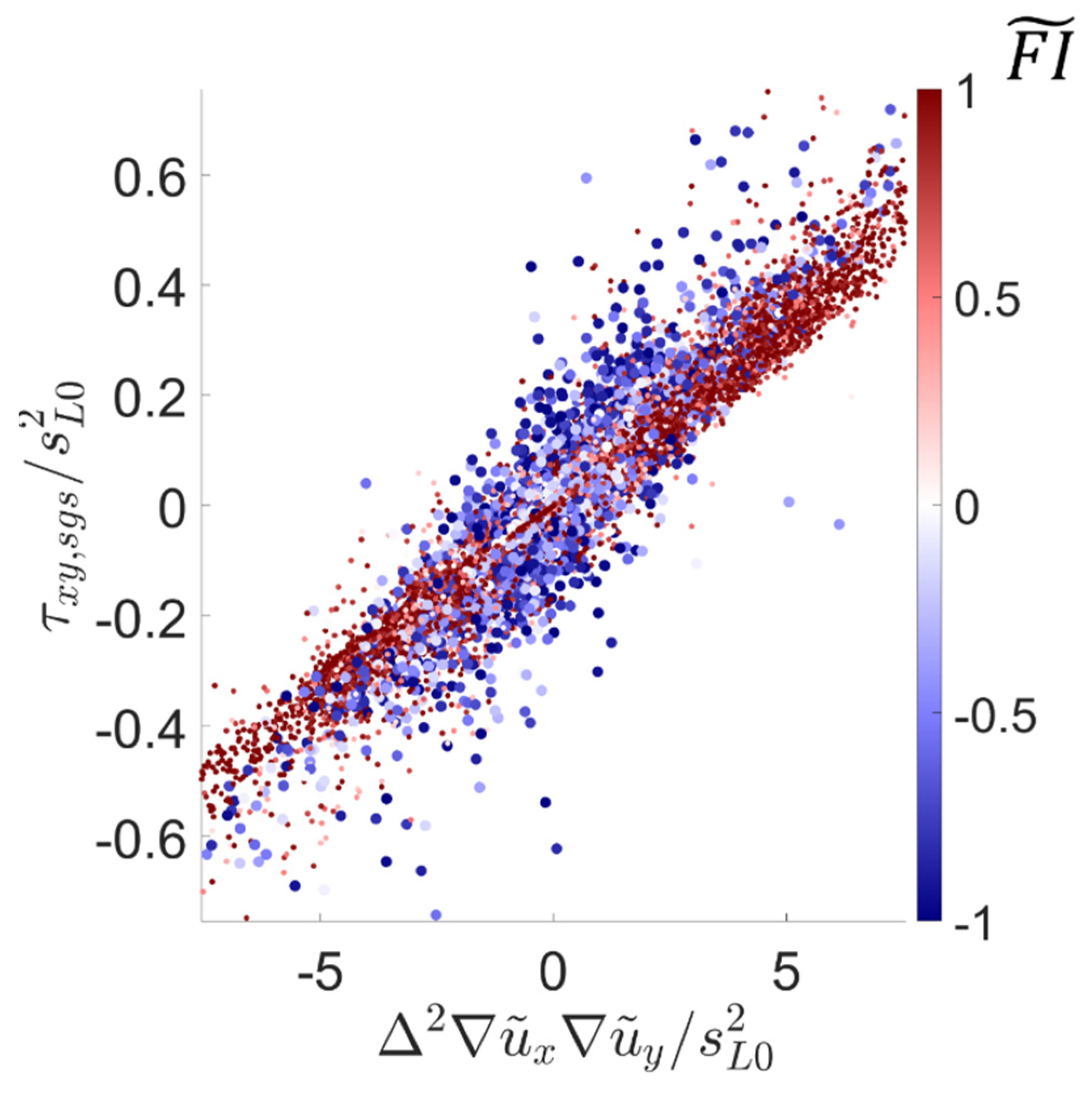
For each recorded timestep, subgrid and filtered quantities are available. The role of an LES model is to predict the former with the latter, using expressions of the sort of (18). For every cell, it is possible to determine the filtered flame index along with the observed subgrid quantities and the elements proposed in this model. Storing this information, it is possible to generate a database like the one presented in
Figure 8. Here, data from a single timestep is displayed to prevent the loss of perspective. However, the actual statistical analyses were performed using data from several timesteps to minimize the statistical error. In the graph of
Figure 8, the vertical axis corresponds to the quantity that has to be modeled (i.e. the subgrid Reynolds stress tensor), whereas the horizontal one contains the model-dependent parameters. The color of each measurement is related to the filtered flame index
. As can be seen, there is a clear correlation between both variables. For each case, the slope of the scattered data cloud corresponds to the model coefficient
, which is used to denote
or
indistinctively. The cells in a premixed regime (
) present a slightly smaller slope compared with the ones that burn in non-premixed conditions (
). This is the motivation for using different coefficients, as mentioned in the previous section.
Figure 6.
Example of instantaneous results for modeling the subgrid stress .
Figure 6.
Example of instantaneous results for modeling the subgrid stress .
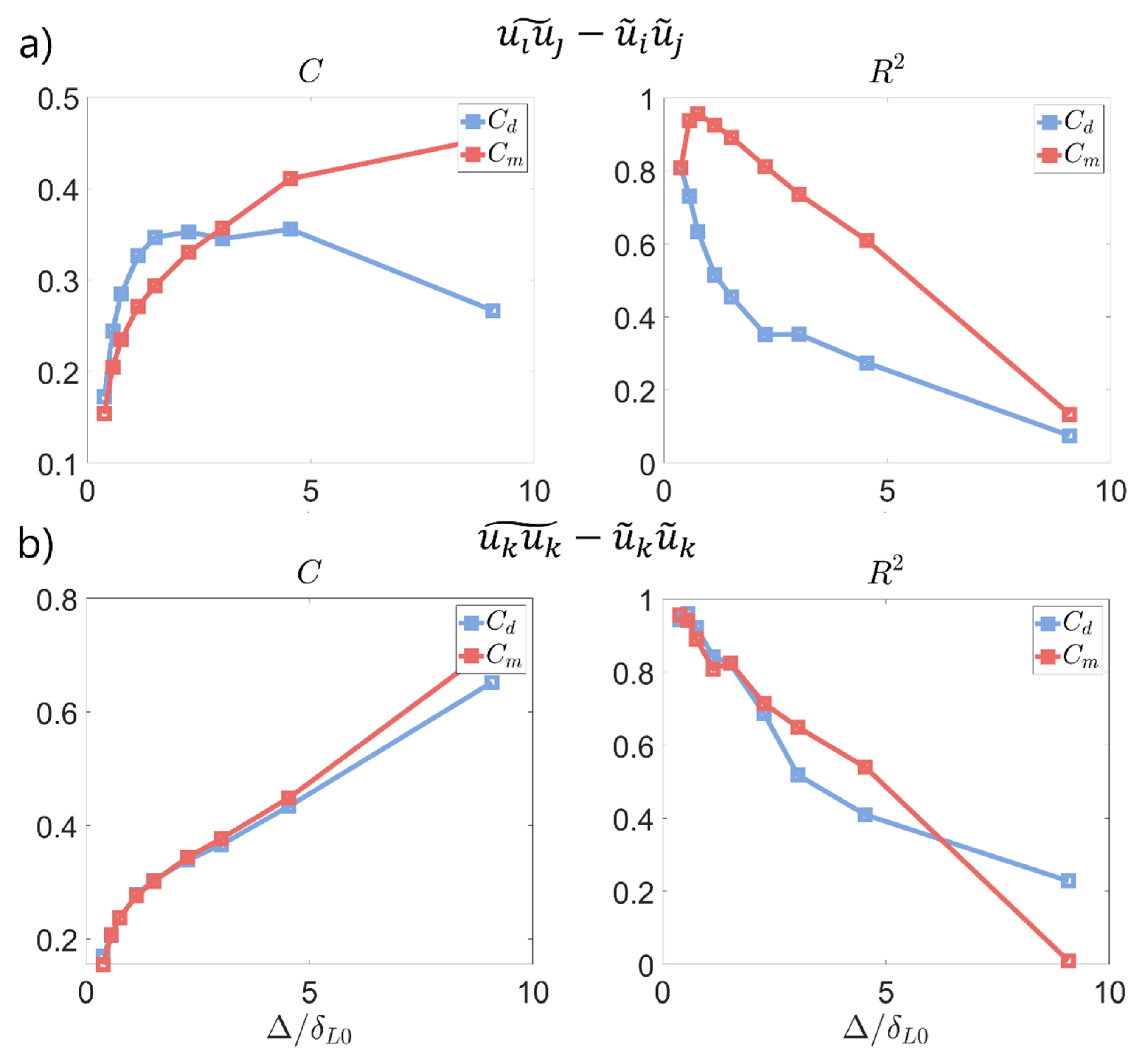
Besides the different sensitivities, it is evident that dispersion is greater for the cells in the non-premixed regime. This trend is consistently observed for most of the modeled subgrid fluxes, indicating a worse model performance in the regions where combustion is driven by diffusion. This behavior is probably caused by the fact that microscale mixing plays a significant role in the subgrid dynamics when the flow is locally non-premixed. Since these processes are partially uncoupled with the filtered (i.e. larger scale) quantities, they incorporate additional noise, worsening the model performance. For the different used grid sizes, the model constants at both premixed and non-premixed conditions were fitted using the least squares method. The obtained coefficients and model performance are presented in
Figure 7.
The coefficient of determination
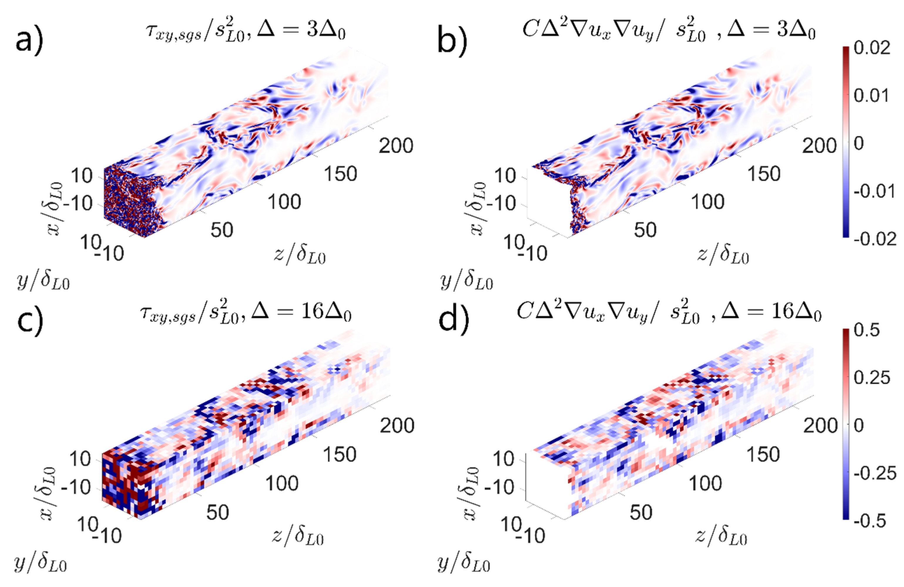
is a valuable indicator of the model quality. However, this parameter is very sensitive to the outlier observations. Hence, it is more convenient to visualize the complete predicted and observed fields as displayed in
Figure 8, to have a more holistic perspective concerning the model performance. In this graph, the measured and modeled subgrid stresses
are presented with different filter widths. For a fine resolution
, the model perfectly predicts the subgrid stress, as one could expect from
. For the filter width
the model has an average coefficient of determination in the order
. Although noticeable disparities appear at certain locations, the model accurately captures the subgrid quantities both quantitatively and qualitatively. In general, for
, the model can be rendered as excellent, and for
, the performance may be classified as good.
Figure 8.
Observed and modeled subgrid Reynolds stress : Observed value with filter width (a), predicted value with filter width (b), observed value with filter width (c), Predicted value with filter width (d).
Figure 8.
Observed and modeled subgrid Reynolds stress : Observed value with filter width (a), predicted value with filter width (b), observed value with filter width (c), Predicted value with filter width (d).
In the inlet regions, there is a significant discrepancy between the model prediction and the observed subgrid stresses. This is caused by the fact that the flow is non-reactive in these locations. This violates the central premise of the developed model. For this reason, points with a filtered progress variable have been excluded from the statistical analysis and model performance evaluations.
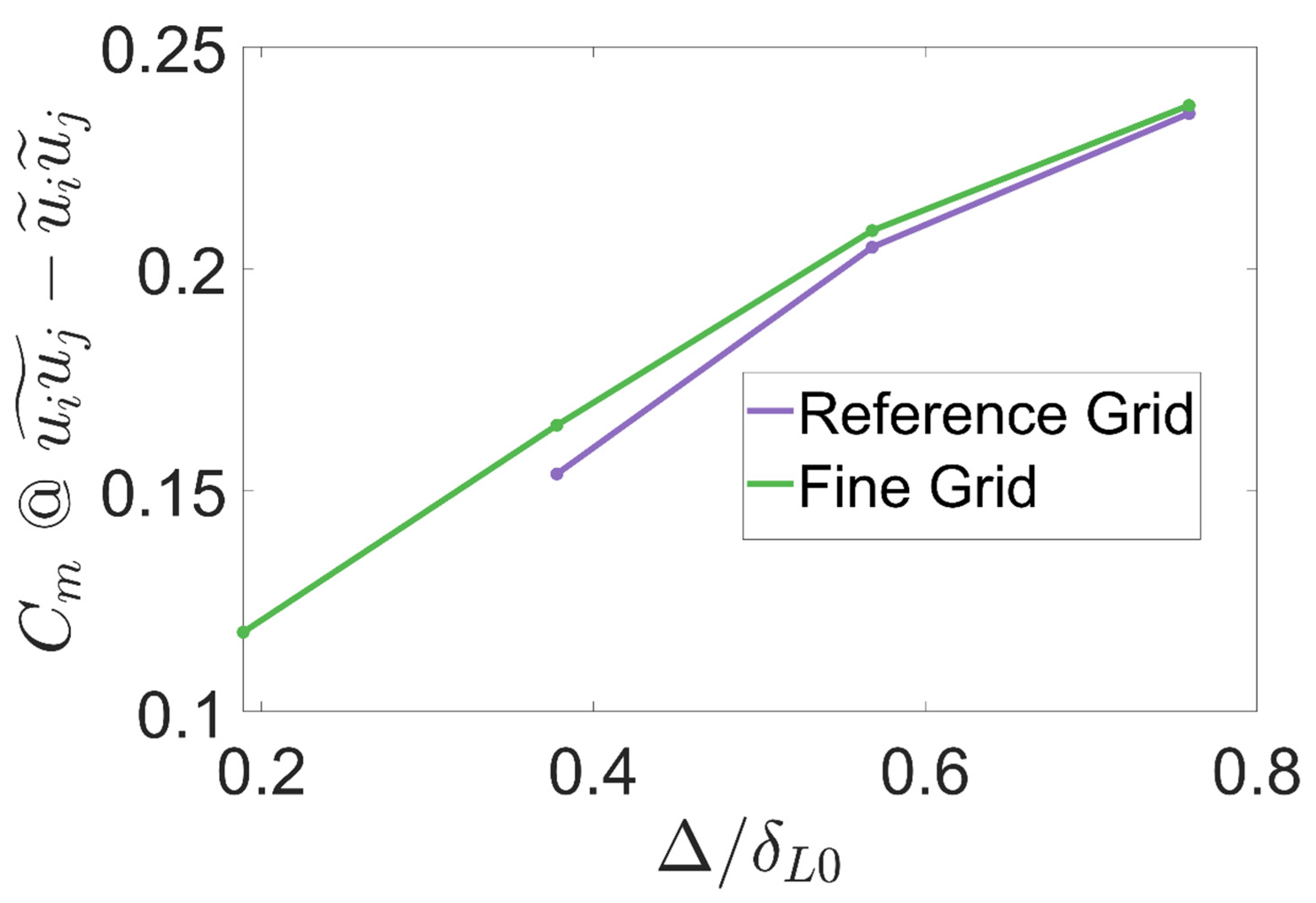
A finer grid has been used to perform a mesh sensitivity analysis over the entire procedure. The grid size of the refined mesh is half the one of the reference DNS. The obtained value for the coefficient
in both the reference simulation and the refined one can be compared in
Figure 9. Only the coefficients for the smaller filter sizes are displayed since the results for larger filters are virtually indistinguishable. As can be seen, there is a minor error in the coefficient for the filter with
. More specifically, the finer grid provides a value a 6.1 % larger compared to the reference case, for the smallest filter width. This increase originates from the small amount of unresolved turbulent processes in the reference case. The discrepancy between the reference case and the one with a refined grid tends asymptotically to zero as larger filter widths are considered, illustrating that the amount of subgrid information contained in both simulations is virtually identical.
Due to the large computational cost and manipulation complexity of the finer database, the mesh sensitivity analysis was only performed over the subgrid Reynolds stress tensor. Nonetheless, these results prove that the reference grid size is small enough to ensure accurate results.
4.2.2. Enthalpy Flux
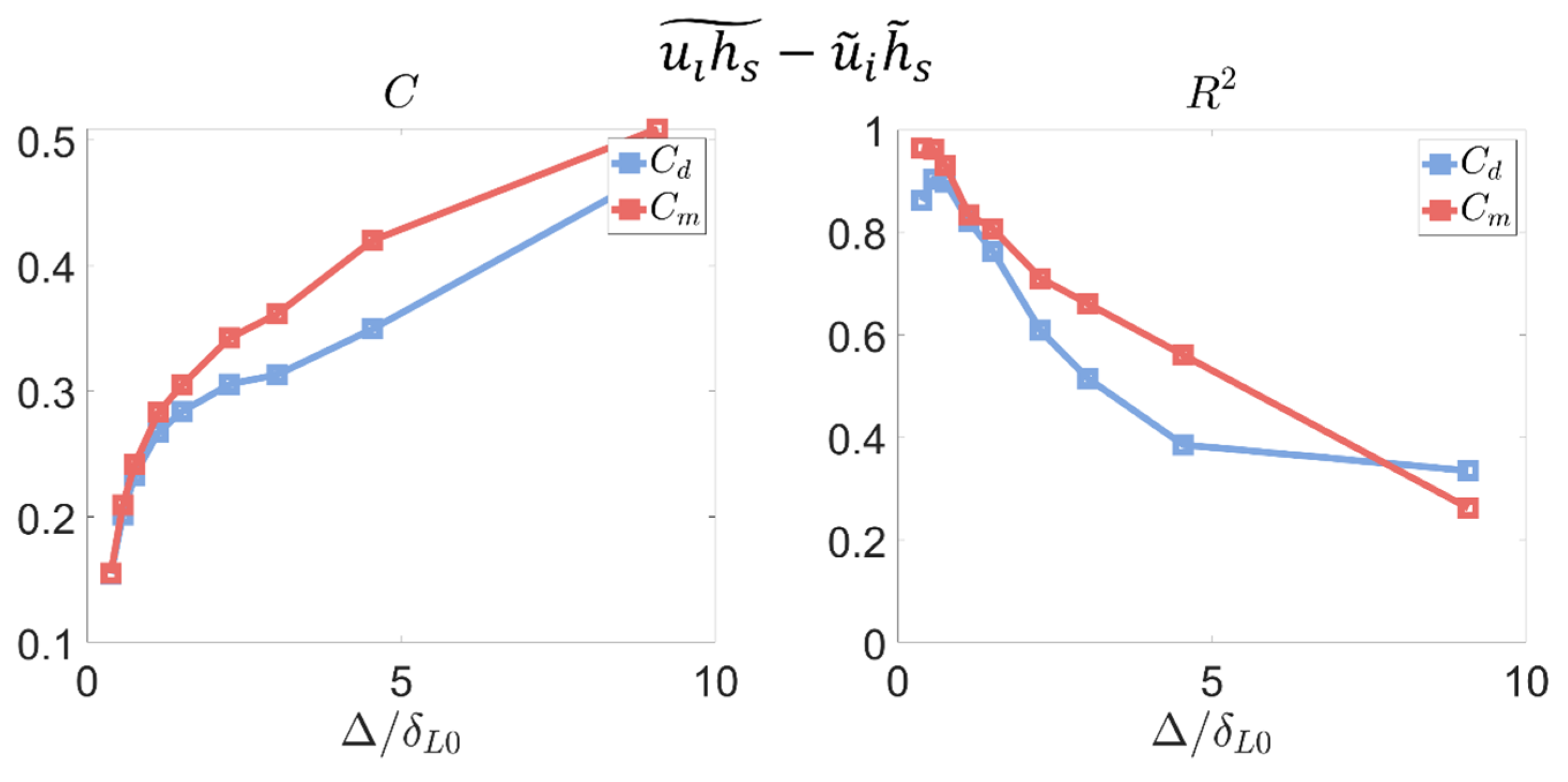
The subgrid enthalpy flux is one of the many terms that require modeling in the energy conservation equation. The devised model was fitted following the previously described procedure. The model constants and behavior present similar values to those obtained for the Reynolds stresses for small filter widths. The main difference between these results and the ones reported for the subgrid Reynolds stresses is that the model constants and performance are more alike for premixed and non-premixed conditions. This similarity is probably caused by the greater sensitivity of Reynolds stresses to composition changes. Microscale mixing processes have an immediate effect on the subgrid Reynolds stresses due to the viscosity differences. The conversion of mixing variability into enthalpy changes requires chemical reactions, which are limited by the local mixture fraction. This additionally required step can dampen the disruptive effect of microscale mixing into the model performance.
Figure 10.
Coefficients and model performance for the subgrid enthalpy flux.
Figure 10.
Coefficients and model performance for the subgrid enthalpy flux.
4.2.3. Species Fluxes
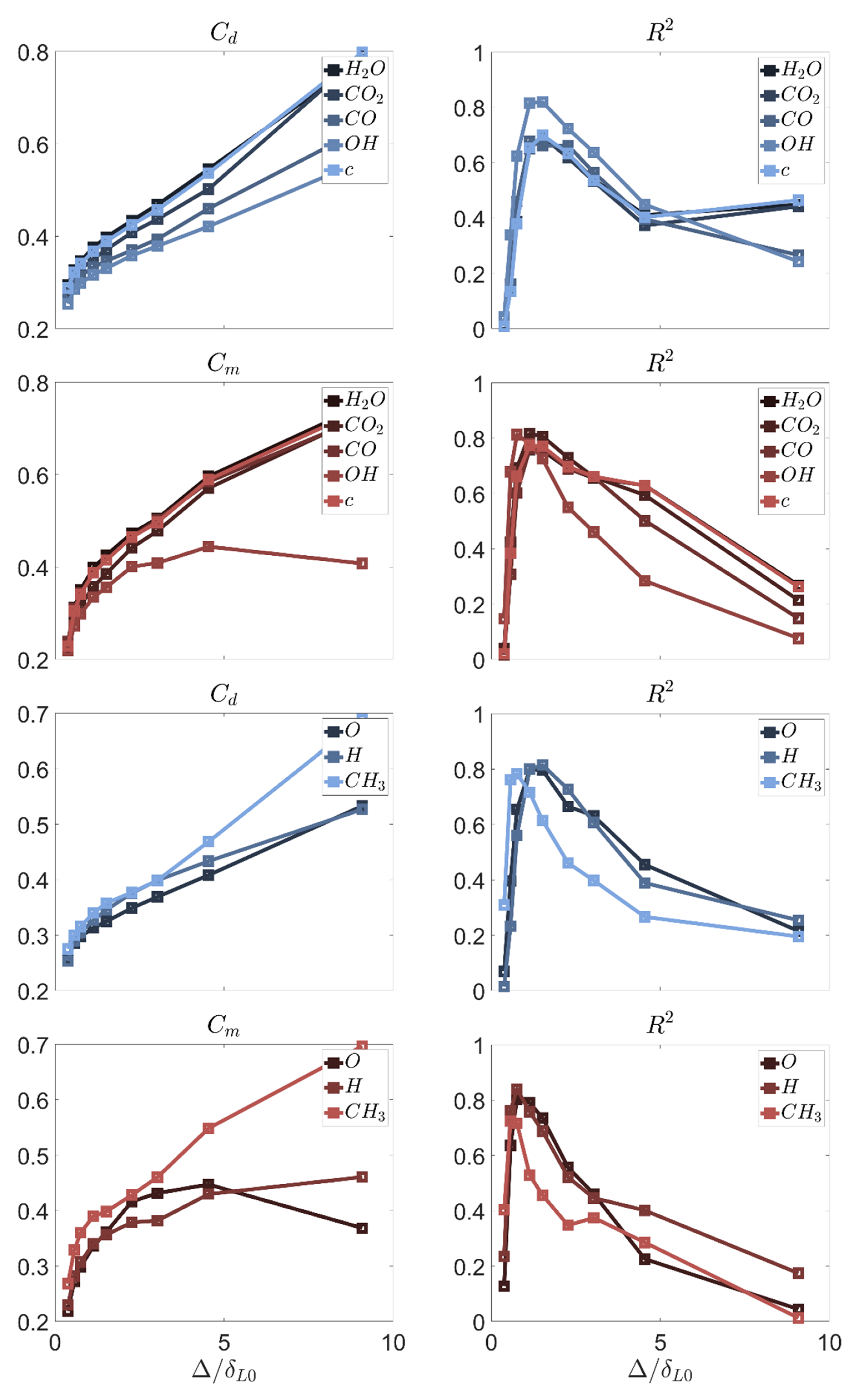
The investigation of the error performance for unresolved species fluxes is significantly challenging. A comprehensive approach would require considering every chemical species in the reaction mechanism. To prevent the loss of sight, only a few selected species are analyzed. The analysis is divided into major species and intermediate i.e., minor species. The summary of the performed adjustment is displayed in
Figure 11. The most relevant difference with the previously reported results is the model performance at small filter widths. This result might appear counterintuitive at first impression. If small grid sizes are considered, the behavior of some quantities is almost laminar, and some unresolved terms tend to be zero. Hence, the fitting problem
has to be solved in a scenario where
and
converge to zero. The low model performance is caused by the ill-posed nature of this mathematical problem in such a context. To verify this claim, the negligibility of the unresolved fluxes has to be demonstrated. With this goal in mind, the following indicator of the subgrid scale fluxes intensity is defined:
which tends to zero when no subgrid modeling for the flux of the quantity
is required. This parameter was evaluated for the subgrid water flux at different filter widths. For
ranges from
to
through all the domain, with a median value
. These results indicate the negligibility of scalar flux at the specified filter width. Neglecting any modeling would have a minimal impact on the species conservation transport equation. For
, the subgrid scale intensity becomes relevant, with
presenting a median value
, which justifies the need for modeling. With this filter width, the model works already very well with
depending on the considered species.
In the analysis summarized in
Figure 11, there appears to be no significant difference between the major and minor species. However, for premixed combustion conditions, the growth of the model coefficient
for species
and
appears to stop after
. The profile of these species strongly depends on the local mixture fraction, and it has a non-monotonic profile through the flame front. These circumstances may decrease the correlation between the resolved processes and the subgrid dynamics. One possible solution would be to consider different coefficients for lean and fuel-rich conditions, enabling adaptation to the varying chemistry behavior in these contexts.
4.3. Dynamic Model Formulation
The previous analyses revealed an important sensitivity of the model coefficients
to the grid size
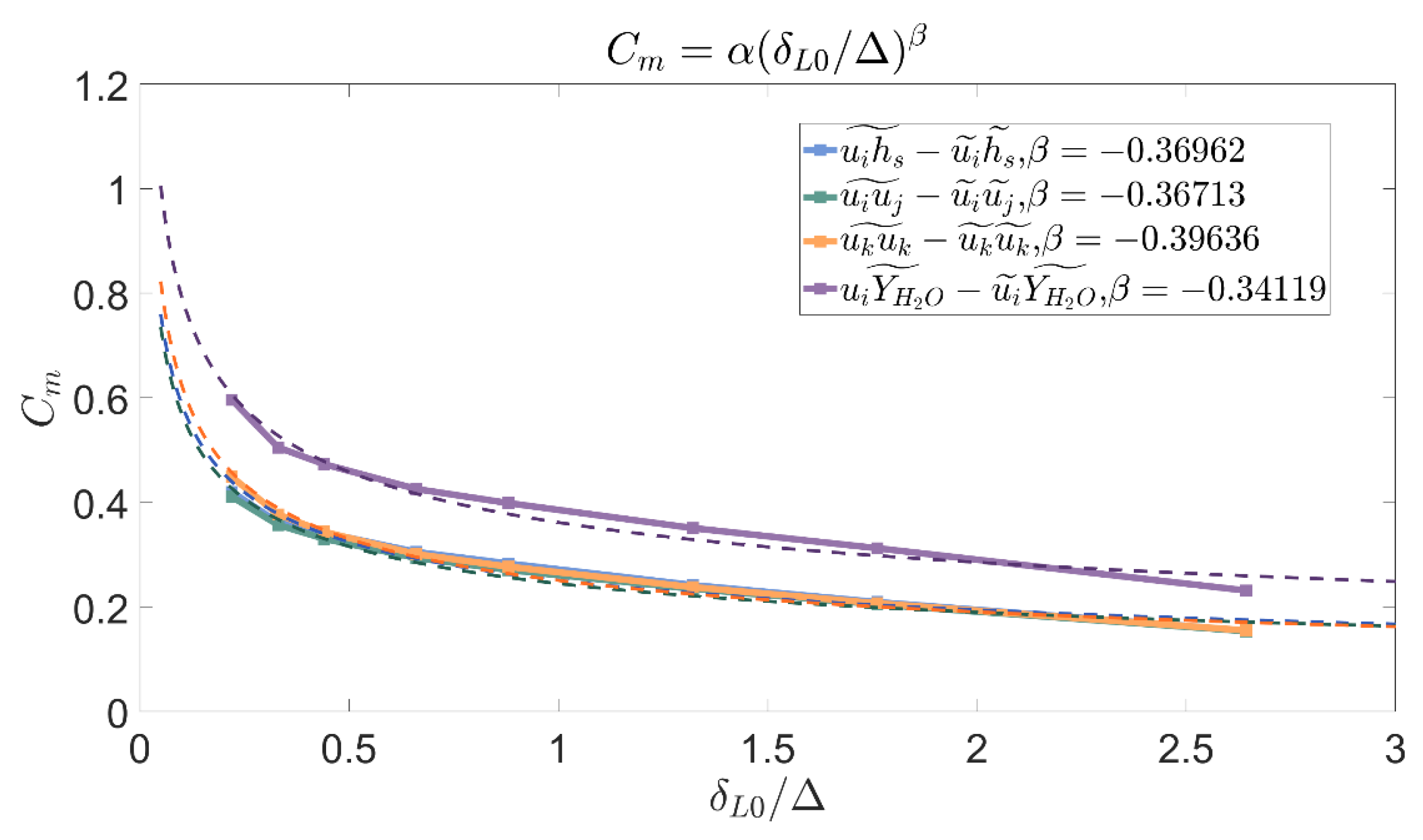
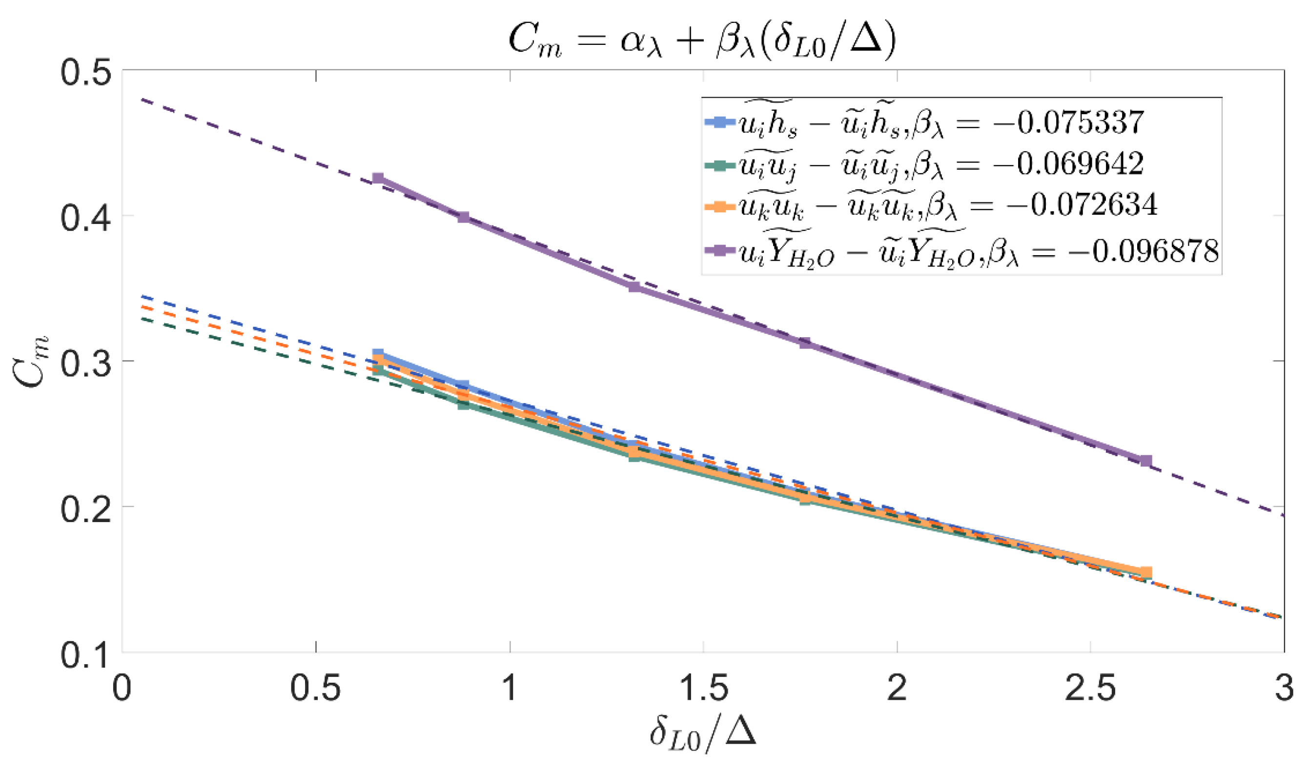
. This dependency can be addressed with a dynamic approach, in which the problem is resolved and filtered with a coarser filter width to derive the model coefficients. However, scaling laws are needed to determine the coefficients at the targeted resolution. The scaling laws for the model coefficients is studied in the present section using the available results. The behavior of coefficient
for premixed combustion (i.e.
) as a function of the grid size
is provided in
Figure 12 for different subgrid fluxes. Due to its similarity, the function of the coefficient
is not reproduced to prevent overclutter. As can be seen, the coefficient follows identical trends for all the unresolved fluxes. This result hints the existence of a universal power law dependency with a value
. If this parameter is known a priori, results at test levels can be used to determine
in (21), and consequently obtain the functions
and
.
For small filter widths, a noticeable deviation with respect to the main trend can be observed. More specifically, the function appears to become linear for
. Hence, a linear modeling of the sort
appears to be better suited in these cases. The results of assuming this dependency for the constant modeling can be visualized in
Figure 13. As it can be seen, linearization provides an almost perfect fitting for the region where the grid size is smaller than the laminar flame front thickness at stoichiometric conditions
.
Based on these results, if the filter width is known to be smaller than the laminar flame thickness, a linear dependency should be assumed. One drawback of this approach is that it requires performing two different tests at already small filter widths, which can be computationally expensive. This problem can be circumvented by linking the behavior in the linear region (
) with the universal dependency law. If
continuity is assumed for
then the derivatives of both models should meet at the transition point
:
where
indicates the filter width at which the transition from potential to linear law occurs. The continuity condition can be used to obtain
as a function of this point
In this approximation, it was assumed that the transition filter width corresponds to the laminar flame thickness at stoichiometric conditions. The validity of this premise can be tested with the available results. With the obtained values for
in
Figure 12, if we set
,
and
are obtained for the steam mass fraction flux and the other unresolved fluxes. These values provide a rather small discrepancy when compared with the actual sensitivity coefficients displayed in
Figure 13. The expression in (24) provides an almost perfect prediction for the coefficients
if the transition filter width is taken as
, which indicates that the change to a linear regime occurs for scales slightly narrower than the laminar flame thickness at stoichiometric conditions. This statement can be qualitatively verified attending to
Figure 13.
The discussed variations in the function
embed profound physical motivations. It shall be considered that the size of the realized flamelets
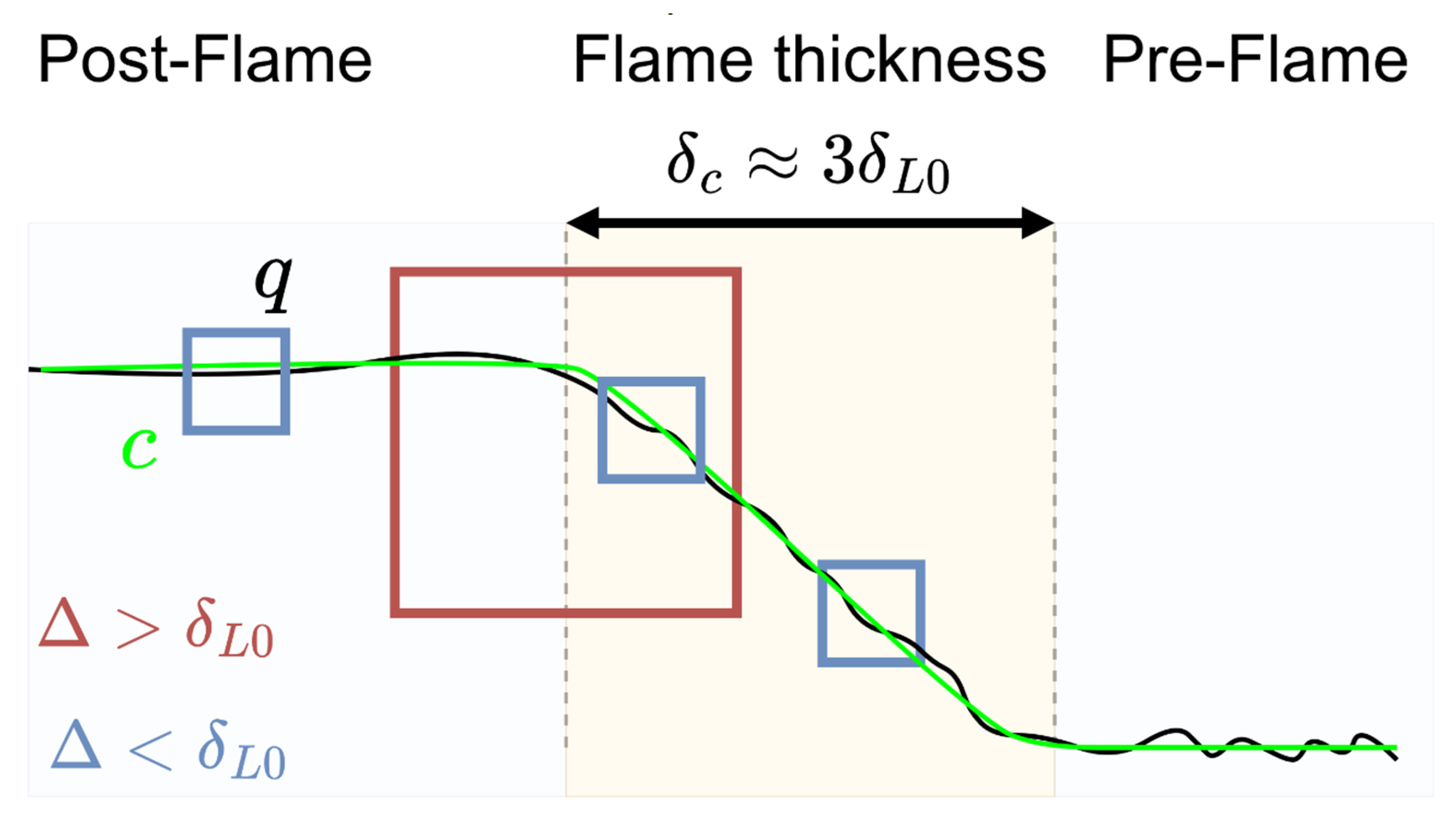
is roughly 3 times larger than laminar flame thickness at stoichiometric conditions. Hence, the found threshold maybe rewritten as roughly
. If The filter width is significantly smaller than the flame thickness, it is safe to assume that the filtering operator
is entirely applied either within the flame or outside it. In such cases, there is consistency between the dynamics at a subgrid level and at large scales. For larger values, the possibility of applying the filter in regions which are only partially reactive becomes relevant. In this scenario, the existence of different subgrid dynamics of reactive and non-reactive zones degrades the similarity between subgrid fluxes and filtered quantities. This effect is displayed in the schematic of
Figure 14. If the filter width is significantly smaller than the reaction thickness, then it is likely to be applied within a volume which falls entirely either within or outside the flame.
5. Validation with
The development and fitting of the presented model is based on the individual evaluation of instantaneous subgrid fluxes. However, it is relevant to investigate the integral performance of the proposed model in the frame of a complete numerical simulation. This section is devoted to the assessment of the model’s global validity using a reference DNS database.
5.1. Simulation Description
The case chosen for the global validation is a recessed methane-oxygen injector which has been studied in recent research works [
80,
101]. These simulations recreate the turbulent combustion in methane – oxygen injectors, using realistic geometrical features, and have been validated with experimental data in a comparable setup. The proposed models in this paper are limited to subgrid fluxes. Despite their remarkable relevance, there are multiple additional unresolved subgrid statistics defining the transient development of the conservation equations. The strong intertwining between the various unclosed terms complicates the global assessment of the enhancements in numerical accuracy provided by an improvement in the subgrid turbulent flux modelling. The following three simulations were used in the present study to investigate the sensitivity of the numerical accuracy to the usage of subgrid adaptive gradient models:
Direct numerical simulation (DNS).
Large eddy simulation with no modelling of subgrid turbulence ().
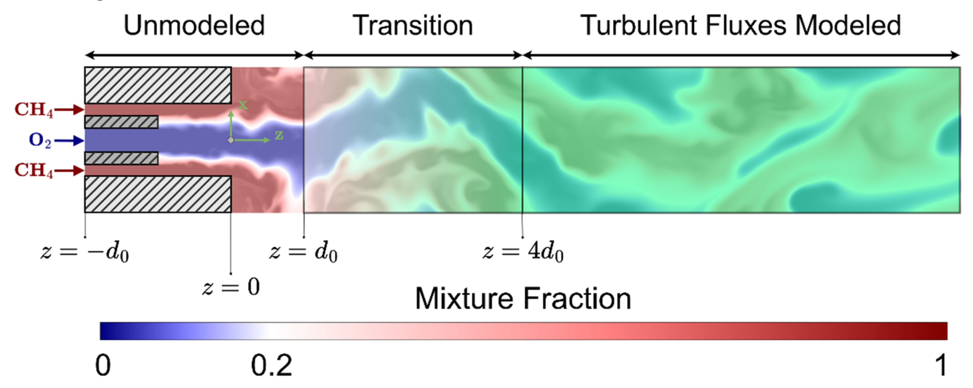
Large eddy simulation with modelling of subgrid turbulence at downstream positions ().
The simulation uses no modelling at all for subgrid quantities, and it is essentially DNS with insufficient resolution. The third simulation i.e. models the subgrid fluxes with the models presented in the previous section at downstream positions. Both simulations , and use a grid size .
The model coefficients take the following value:
where
, and
are coefficients defining the local application of the subgrid models, and
is the reference coefficient for the modelled subgrid flux. The coefficient
controls the restriction of the model application to reactive regions using the following formulation:
Which enables a smooth transition from the non-reactive to the reactive case. The factor
is devised in a similar fashion, defining a transition from
to
, as illustrated in
Figure 15:
The main motivation of this transition is to avoid the application of the presented model in regions close to walls, where dedicated treatment of wall turbulence is better approached with other alternatives.
5.2. Results Comparison
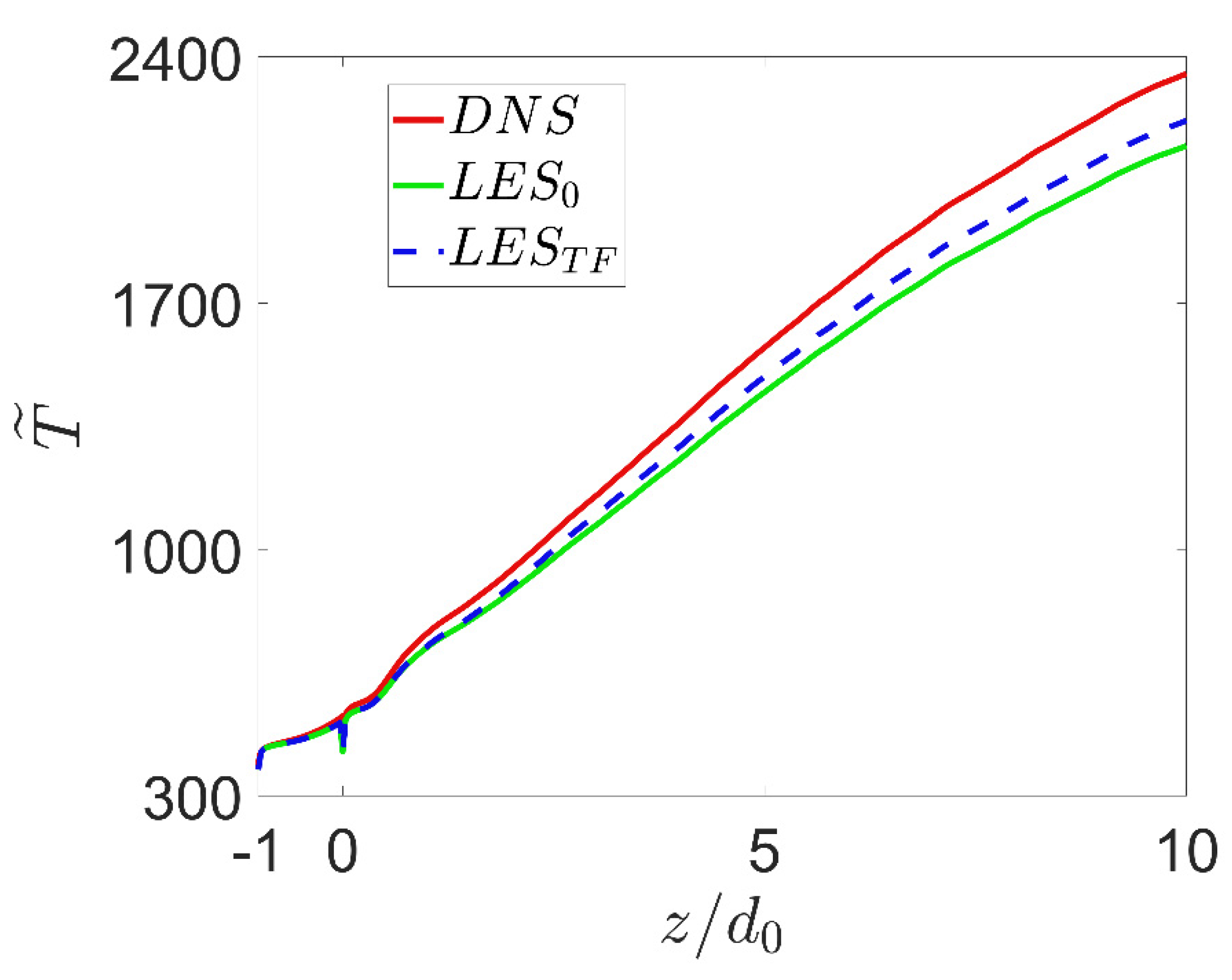
The average temperature over time and radial direction is used to compare the output of the different simulations. This scalar can be taken as a robust marker of the overall combustion development. The axial evolution of this quantity for the three considered simulations is displayed in
Figure 16. As can be seen, the complete neglection of subgrid effects is translated into a substantial underprediction of the combustion progress (
). This is caused by the insufficiently small grid size which effectively reduces the turbulent Reynolds number, thereby suppressing microscale diffusion and mixing. The incorporation of the models for subgrid turbulent fluxes increases the axial temperature gradient, bringing the DNS and
outputs closer. Nonetheless, a steady state offset between these two simulations remains. This discrepancy is attributed to absence of any modelling within
, and the unresolved subgrid quantities that are not turbulent fluxes, which remain non-modelled through all the domain of the simulation
. These results demonstrate the capability of the presented gradient models to improve the accuracy of LES in reactive turbulent flows.
6. Conclusions and Outlook
The present research has addressed the application of the gradient model for subgrid turbulent fluxes in turbulent combustion conditions representative of space propulsion applications. An extension of the gradient model considering the local burning regime has been introduced. Hence, the determination of subgrid covariances depends on whether combustion takes place at premixed or non-premixed conditions. It is found that the gradient model performs significantly better if combustion is locally premixed, and that the magnitude of subgrid fluxes is slightly greater in zones where combustion occurs in non-premixed conditions. These trends are attributed to the lower complexity of premixed flamelets compared to the ones driven by diffusion. Since mixing is required for the development of non-premixed flamelets, the subgrid dynamics have a greater potential to decoupled from the processes at larger scales, reducing the model’s validity. The dependency of the model’s coefficients on the grid size was studied comparing the fitted values for different subgrid fluxes. For filters widths below the laminar flame thickness at stoichiometric conditions (), a linear sensitivity of the model coefficients with respect to the filter widths is found. This linearity degrades if filter widths larger than are considered, and a power law in the order provides a good general fitting. This change is attributed to the simultaneous presence of various flame regions at a subgrid level, which decouples the small- and large-scale dynamics. Overall, the proposed model can predict subgrid turbulent fluxes with high precision for filter widths up to twice the laminar flame thickness at stoichiometric conditions. The validity of the presented models has been investigated in complete Large Eddy Simulations as well. It was found that the introduction of subgrid gradient models at positions sufficiently far away from the walls improves numerical accuracy. Future research works shall apply the proposed methodology at different combustion conditions with different turbulent and chemical dynamics to assess the universality of the presented models.
Author Contributions
Conceptualization, D.M.S. and A.S.; methodology, D.M.S.; software, D.M.S. , A.S. and S.B.; validation, D.M.S., A.S. and S.B.; formal analysis, D.M.S and O.H..; investigation, D.M.S. and S.B.; resources, D.M.S, A.S., O.H. and M.T.; data curation, D.MS. and S.B; writing—original draft preparation, D.M.S and A.S.; writing—review and editing, O.H..; visualization, D.M.S..; supervision, O.H. and M.T.; project administration, A.S. and O.H. All authors have read and agreed to the published version of the manuscript.
Funding
This research received no external funding
Data Availability Statement
Data can be provided upon reasonable request.
Acknowledgments
The authors are thankful to the Leibniz RechenZentrum (LRZ) for the provided computational resources with SMUC Ngen. The authors want to thank Marten Ohlerich for his dedication and continuous support which contributed to the optimization of computational resources. The authors are grateful to Eiki Mori for his support in adapting the solver EBI-DNS for partial LES capabilities.
Conflicts of Interest
The authors declare no conflict of interest.
References
- D. Haeseler, V. Bombelli, P. Vuillermoz, R. Lo, T. Marée und F. Caramelli, „Green Propellant Propulsion Concepts for Space Transportation and Technology Development Needs,“ in 2nd Inernational Conference on Green Propellants for Space Propulsion, Chia Laguna (Cagliari), 2004.
- R. L. Sackheim und R. K. Masse, „Green Propulsion Advancement - Challenging the Maturity of Monopropellant Hydrazine,“ in 49th AIAA Joint Propulsion Conference, San Jose, CA USA, 2013. [CrossRef]
- D. Preclik, G. Hagemann, O. knab, C. Mading, D. Haeseler, O. J. Haidn, A. Woschnak und M. DeRosa, „Lox-hydrocarbon preparatory thrust chamber technology activities in Germany,“ in 41st AIAA/ASME/SEA/ASEE Joint Propulsion Conference & Exhibit, Tucson, Arizona, 2005.
- O. Haidn, G. Ordonneau, S. Soller und M. Onofri, „Oxygen-Methane Combustion Studies in the In Space Propulsion Programme,“ in 4th European Conference for Aerospace Sciences, Saint Petesbourg, Russia, 2011.
- O. J. Haidn, M. P. Celano, M. Luo, C. Roth, S. Silvestri und N. A. Slavinskaya, „On Methane/ Oxygen Combustion for Rocket Applications,“ in International Symposium on Innovation and Prospects of Liquid Propulsion, Xi'an, China, 2016.
- P. K. Tucker, S. Menon, C. Merkle, J. Oefelein, Yang und Vigor, „An approac to Improved Credibility of CFD Simulations for Rocket Injector Design,“ in 43rd AIAA/ASME/SAE/ASEE Joint Propulsion Conference & Exhibit, Cincinnati OH, 2007.
- Y.-D. Kang und B. Sun, „Numerical Simulation of Liquiud ROcket Engine Thrust Chamber Regenerative Cooling,“ Journal of Thermophysics and Heat Transfer, Bd. 25, Nr. 1, pp. 155-164, 2011. [CrossRef]
- Y. Daimon, H. Negishi, M. Koshi und D. Suslov, „Numerical and Experimental Investigation of the Methane Film Cooling in Subscale Combustion Chamber,“ in 5th European Conference for Aeronautics and Space Sciences (EUCASS), Munich, Germany, 2013.
- V. Zubanov, V. Egorychev und L. Shabliy, „Design of Rocket Engine for Spacecraft Using CFD-Modeling,“ Procedia Engineering, Bd. 104, pp. 29-35, 2015. [CrossRef]
- N. Perakis, D. Rahn, O. J. Haidn und D. Eiringhaus, „Heat Transfer and Combustion Simulation of Seven-Element O2/CH4 Rocket Combustor,“ Journal of Propulsion and Power, Bd. 35, Nr. 1, pp. 1-18, 2019. [CrossRef]
- A. Sternin, M. Hao, O. J. Haidn und M. Tajmar, „Turbulence and Combustion and Film Prediction in Rocket Application via Parameter Adjustment, Model Variation and Deep Learning Method,“ in DFG TRR40 Summer Program, 2019.
- P. Breda, J. Zips und M. Pfitzner, „A Non-Adiabatic Flamelet Approach for Non-Premixed O2-CH4 Combustion,“ in proceedings of the 3rd World Congress on Momentum, Heat and Mass Transfer, Budapest, Hungary, 2018.
- M. Pizzarelli, N. F und M. Onofri, „Evolution of Cooling-Channel Properties for Varying Aspect Ratio,“ Progress in Propulsion Physics, Bd. 8, pp. 117-128, 2016.
- M. Pizzarelli, B. Betti und F. Nasuti, „Coupled analysis of hot-gas and coolant flows in LOX/methane thrust chambers,“ in 4th European Conference for Aerospace Sciences, Saint Petersburg, 2011.
- A. Sternin, N. Perakis, M. P. Celano und O. Haidn, „CFD-analysis of the effect of a cooling film on flow and heat transfer characteristics in a GCH4/GOX rocket combustion chamber,“ in Space Propulsion 2018, Sevilla, 2018.
- J. Liu, S. Zhang, J. Wei und O. J. Haidn, „RANS based numerical simulation of a GCH4/GO2 rocket engine combustion chamber with film cooling and improvement of wall heat flux prediction,“ Applied Thermal Engineering, Bde. %1 von %2219, Part B, 2023.
- I. Nasser, O. Haidn und C. Manfletti, „Numerical Investigation of Rocket Engine Cooling Channel Heat Transfer for Different LNG Under Trans-Critical Conditions,“ International Journal of Thermofluids, Bd. 20, p. 100461, 2023. [CrossRef]
- C. A. Z. Towery, A. Y. Poludnenko, J. Urzay, J. O'Brien, M. Ihme und P. E. Hamlington, „Spectral kinetic energy transfer in turbulent premixed reacting flows,“ Physical Review, Bd. E93, p. 053115, 2016. [CrossRef]
- J. Furukawa, Y. Noguchi, T. Hirano und F. A. Williams, „Anisotropic enhancement of turbulence in large-scale, low intensity turbulent premixed propane-air flames,“ Journal of FLuid Mechanics, Bd. 462, pp. 209-243, 2002.
- B. Karlovitz, D. W. Denniston und F. E. Wells, „Investigation of turbulent flames,“ Journal of Chemical Physics, Bd. 19, Nr. 5, pp. 541-547, 1951. [CrossRef]
- K. N. C. Bray, P. A. Libby, G. Masuya und J. B. Moss, „Turbulence Production in Premixed Turbulent Flames,“ Combustion Science and Technology, Bd. 25, Nr. 3-4, pp. 127-140, 1981. [CrossRef]
- D. R. Ballal, „Combustion-Generated Turbulence in Practical Combustors,“ in 23rd Joint Propulsion Conference, SanDiego, CA, 1987. [CrossRef]
- A. Gulati und J. F. Driscoll, „Flame-generated Turbulence and mass fluxes: Effect of varying heat release,“ in Symposium (International) on Combustion, 1986. [CrossRef]
- L. Vervisch, P. Domingo, J. Reveillon, S. Payet, C. Pera und R. Hauguel, „DNS and LES of Turbulent Combustion,“ in Computational Fluid Dynamics in Chemical Reaction Engineering IV, Barga, Italy, 2005.
- W. Rodi, „DNS and LES of some Engineering Flows,“ Fluid Dynamics Research, Bd. 38, Nr. 2, pp. 145-173, 2006. [CrossRef]
- G. Pont, P. Brenner, P. Cinnella und J.-C. Robinet, „High-Order hybrid RANS/LES strategy for industrial applications,“ in Direct and Large-Eddy Simulation X, Springer, Cham, 2018, pp. 313-319.
- K. Fujii, „Progress and future prospects of CFD in aerospace- Wind tunnel and beyond,“ Progress in aerospace sciences, Bd. 41, Nr. 6, pp. 455-470, 2022. [CrossRef]
- T. Poinsot und D. Veynante, „Introduction to turbulent combustion,“ in Theoretical and Numerical Combustion, 2005, pp. 125-181.
- A. Y. Poludnenko und E. S. Oran, „The interaction of high-speed turbulence with flames: Global properties and internal flame structure,“ Combustion and Flame, Bd. 157, Nr. 5, pp. 995-1011, 2010. [CrossRef]
- O. Colin, F. Ducros, D. Veynante und T. Poinsot, „A thickened flame model for large eddy simulations of tubulent premixed combustion,“ Physics of Fluids, Bd. 12, pp. 1843-1863, 2000. [CrossRef]
- B. Cuenot, F. Shum-Kivan und S. Blanchard, „The thickened flame approach for non-premixed combustion: Principles and implications for turbulent combustion modeling,“ Combustion and Flame, Bd. 239, p. 111702, 2022. [CrossRef]
- D. Maestro, B. Cuenot und L. Selle, „Large Eddy Simulation of Combustion and Heat Transfer in a Single Element GCH4/GOX Rocket Combustor,“ Flow, Turbulence and Combustion, Bd. 103, Nr. 5, 2019. [CrossRef]
- H. Pitsch, „Large-eddy simulation in turbulent combustion,“ Annual Review of Fluid Mechanics, Bd. 38, pp. 453-482, 2006.
- C. Fureby, „Large eddy simulation modelling of combustion for propulsion applications,“ Philosophical Transactions of the Royal Society, Bd. 367, pp. 2957-2969, 2009. [CrossRef]
- O. Colins, F. Ducros und D. Veynante, „A thickened flame model for large eddy simulations of turbulent premixed combustion,“ Physics of Fluids, Bd. 12, Nr. 7, pp. 1843-1863, 2000. [CrossRef]
- F. Charlette, C. Meneveau und D. Veynante, „A power-law flame winkling model for LES of premixed turbulent combustion part I: non-dynamic formulation and initial tests,“ Combustion and Flame, Bd. 131, Nr. 1-2, pp. 159-180, 2002. [CrossRef]
- O. Rathore und S. Navarro-Martinez, „Flame Dynamics Modelling Using Artificially Thickened Models,“ Flow, Turbulence and Combustion, 2023. [CrossRef]
- H. Pitsch, „A G-equation formulation for large-eddy simulation of premixed turbulent combustion,“ Center for Turbulence Research, Annual Research Briefs 2002, 2002.
- H. Pitsch und L. Duchamp de Lageneste, „Large-eddy simulation of premixed turbulent combustion using a level-set approach,“ Proceedings of the Combustion Institute, Bd. 29, Nr. 2, pp. 2001-2008, 2002. [CrossRef]
- E. R. Hawkes und R. Cant, „A flame surface density approach to large-eddy simulation of premixed turbulent combustion,“ Proceedings of the Combustion Institute, Bd. 28, Nr. 1, pp. 51-58, 2000. [CrossRef]
- R. A. Clark, J. H. Ferziger und W. C. Reynolds, „Evaluation of subgrid-scale models using an accurately simulated turbulent flow,“ Journal of Fluid Mechanics, Bd. 91, Nr. 1, pp. 1-16, 2006. [CrossRef]
- B. Vreman, B. Geurts und H. Kuerten, „Large-Eddy Simulation of the Temporal Mixing Layer Using the Clark Model,“ Theoretical and Computational, Bd. 8, pp. 309-324, 1996. [CrossRef]
- C. D. Pierce und P. Moin, „A dynamic model for subgrid-scale variance and dissipation rate of a conserved scalar,“ Physics of Fluids, Bd. 10, Nr. 12, pp. 3041-3044, 1998. [CrossRef]
- P. K. Yeung und S. B. Pope, „Lagrangian statistics from direct numerical simulations of isotropic turbulence,“ Journal of Fluid Mechanics, Bd. 207, pp. 531-586, 1987. [CrossRef]
- A. Favre, „Problems of hydrodynamics and continuum mechanics,“ SIAM, Philadelphia, 1969.
- L. C. Berselli, T. Iliescu und W. J. Layton, „Filtering,“ in Mathematics of Large Eddy Simulation of Turbulent Flows, Springer Berlin, Hedelberg, 2006, pp. 227-251.
- E. Garnier, N. Adams und P. Sagaut, „LES Governing Equations,“ in Large Eddy Simulation for Compressible Flows, Springer Dordrecht, 2009, pp. 5-40.
- J. Smagorinsky, „General Circulation Experiments with the Primitive Equations,“ Monthly Weather Review, Bd. 91, Nr. 3, pp. 99-164, 1963. [CrossRef]
- D. K. Lilly, „On the application of the eddy-viscosity concept in the inertial sub-range of turbulence,“ NCAR, 1966. [CrossRef]
- J. W. Deardorff, „A numerical study of three-dimensional turbulent channel flow at Large Reynolds numbers,“ Journal of Fluid Mechanics, Bd. 41, Nr. 2, pp. 453-480, 1970. [CrossRef]
- U. Piomelli, P. Moin und J. H. Ferziger, „Model consistency in large eddy simulation of turbulent channel flows,“ Physics of Fluids, Bd. 31, Nr. 7, pp. 1884-1891, 1988.
- S. L. Woodruff, J. M. Seiner und M. Y. Hussaini, „Grid-Size Dependence in the Large-Eddy Simulation,“ AIAA Journal, Bd. 38, Nr. 4, pp. 600-604, 2000. [CrossRef]
- Y. D. Sukanta Basu, B. Maronga und S. R. de Roode, „Addressing the Grid-Size Sensitivity Issue in Large-Eddy Simulations of Stable Boundary Layers,“ Boundary-Layer Meteorology, Bd. !/(, pp. 63-89, 2021. [CrossRef]
- C. Meneveau, „Germano identity-based subgrid-scale modeling: A brief survey of variations on a fertile theme,“ Physics of Fluids, Bd. 24, Nr. 12, 2012. [CrossRef]
- A. Yoshizawa, „Statistical theory for compressible turbulent shear flows, with application to subgrid modeling,“ Physics of Fluids, Bd. 29, pp. 2152-2164, 1986. [CrossRef]
- G. Erlebacher, M. Y. Hussaini, H. O. kreiss und S. Sarkar, „The analysis and simulation of compressible turbulence,“ Theoretical and Computational Fluid Dynamics, Bd. 2, pp. 73-95, 1990. [CrossRef]
- T. M. Eidson, „Numerical simulation of the turbulent Rayleigh-Bénard problem using subgrid modelling,“ Journal of Fluid Mechanics, Bd. 158, pp. 245-268, 1985. [CrossRef]
- J. Urzay, J. O'Brien, M. Ihme, P. Moin und A. Saghafian, „Backscatter of turbulent kinetic energy in chemically-reacting compressible flows,“ Center for Turbulence Research, Annual Research Briefs, 2013.
- A. W. Cook und J. J. Riley, „A subgrid model for equilibrium chemistry in turbulent flows,“ Physics of Fluids, Bd. 6, Nr. 8, pp. 2868-2870, 1994. [CrossRef]
- G. Balarac, H. Pitsch und V. Raman, „Development of a dynamic model for the subfilter scalar variance using the concept of optimal estimators,“ Physics of Fluids, Bd. 20, Nr. 3, p. 035114, 2008. [CrossRef]
- E. Knudsen, E. S. Richardson, E. M. Doran und H. Pitsch, „Modeling scalar dissipation and scalar variance in large eddy simulation: Algebraic and Transport equation closures,“ Physics of Fluids, Bd. 24, Nr. 5, p. 055103, 2012. [CrossRef]
- A. W. Cook und W. K. Bushe, „A subgrid-scale model for the scalar dissipation rate in nonpremixed combustion,“ Physics of Fluids, Bd. 11, Nr. 3, pp. 746-748, 1999. [CrossRef]
- N. Peters, Turbulent Combustion, Cambridge: Cambridge University Press, 2001.
- T. Poinsot und D. Veynante, „Turbulent non premixed flames,“ in Theoretical and Numerical Combustion, Bordeaux, France, Aquaprint, 2012, pp. 287-348.
- H. Yamashita, M. Shimada und T. Takeno, „A numerical study on flame stability at the transition point of jet diffusion flames,“ Symposium (International) on Combustion, Bd. 26, Nr. 1, pp. 27-34, 1996. [CrossRef]
- T. Zirwes, F. Zhang, P. Habisreuther, M. Hansinger, H. Bockhorn, M. Pfitzner und D. Trimis, „Identification of Flame Regimes in Partially Premixed Combustion from a Quasi-DNS Dataser,“ Flow, Turbulence and Combustion, Bd. 1006, pp. 373-404, 2021. [CrossRef]
- P. N. Kioni, B. Rogg, K. N. C. Bray und A. Liñán, „Flame spread in laminar mixing layers: the triple flame,“ Combustion and Flame, Bd. 95, Nr. 3, pp. 276-290, 1993. [CrossRef]
- B. Cuenot, „The Flamelet Model for Non-Premixed Combustion,“ in Turbulent Combustion Modelling, 2011, pp. 43-61. [CrossRef]
- K. Bray, P. Domingo und L. Vervisch, „Role of the progress variable in models for partially premixed turbulent combustion,“ Combustion and Flame, Bd. 141, Nr. 4, pp. 431-437, 2005. [CrossRef]
- R. W. Bilger, „Turbulent jet diffusion flames,“ Progress in Energy and Combustion Science, Bd. 1, Nr. 2-3, pp. 87-109, 1976.
- D. Martínez-Sanchis, S. Banik, A. Sternin, D. Sternin, O. Haidn und M. Tajmar, „Analysis of turbulence generation and dissipation in shear layers of methane-oxygen diffusion flames using direct numerical simulations,“ Physics of Fluids, Bd. 34, p. 045121, 2022. [CrossRef]
- D. Martínez-Sanchis, A. Sternin, O. J. Haidn und M. Tajmar, „Turbulent Combustion Statistics in a Diffusion Flame for Space Propulsion Applications,“ Physics of Fluids, Bd. Submitted Paper, 2022. [CrossRef]
- C. D. Pierce und P. Moin, „Progress-variable approach for large-eddy simulation of non-premixed turbulent combustion,“ Journal of Fluid Mechanics, Bd. 504, pp. 73-97, 2004. [CrossRef]
- D. Martínez-Sanchis, A. Sternin, J. Shvab, O. J. Haidn und X. Hu, „An Eddy Dissipation Concept Performance Study for Space Propulsion Applications,“ Aerospace, 2022. [CrossRef]
- D. Martínez-Sanchis, A. Sternin, D. Sternin, O. Haidn und M. Tajmar, „Analysis of periodic synthetic turbulence generation and development for direct numerical simulations,“ Physics of FLuids, Bd. 33, p. 125130, 2021. [CrossRef]
- C. Morsbach und M. Franke, „Analysis of a synthetic turbulence generation method for periodic configurations,“ in Direct and Large-Eddy Simulation XI, Springer International Publishing, 2019, pp. 169-174.
- M. L. Shur, P. R. Spalart, M. K. Strelets und A. K. Travin, „Synthetic Turbulence Generators for RANS-LES Interfaces in Zonal Simulations of Aerodynamic and Aeroacoustic Problems,“ Flow, Turbulence and Combustion, Bd. 93, pp. 63-92, 2014. [CrossRef]
- R. H. Kraichnan, „Diffusion by a Random Velocity Field,“ The Physics of Fluids, Bd. 13, pp. 22-31, 1970. [CrossRef]
- D. Martinez-Sanchis, A. Sternin, T. Santese und O. J. Haidn, „The role of turbulence in the characteristic velocity of rocket combustors,“ Aerospace Science and Technology, Bd. 134, p. 108158, 2023. [CrossRef]
- D. Martinez-Sanchis, A. Sternin, A. Jocher und O. Haidn, „Analysis of Turbulent Mixing in a Methane - Oxygen Recessed Injector for Space Propulsion,“ Physics of Fluids, 2023. [CrossRef]
- F. Zhang, H. Bonart, T. Zirwes, P. Habisreuther und Bockhorn, „Direct numerical simulations of chemically reacting flows with the public domain code OpenFOAM,“ in High Performance Computing in Science and Engineering '16, Bd. 14, Springer, 2015, pp. 221-236. [CrossRef]
- T. Zirwes, F. Zhang, J. Denev, P. Habisreuther und H. Bockhorn, „Automated code generation for maximizing performance of detailed chemistry calculations in OpenFOAM,“ in High Performance Computing in Science and Engineering '17, Springer, 2018, pp. 189-204. [CrossRef]
- T. Zirwes, F. Zhang, J. A. Denev, P. Habisreuther, H. Bockhorn und D. Trimis, „Improved vectorization for efficient chemistry computations in OpenFOAM for large scale combustion simulations,“ in High Performance Computing in Science and Engineering '18, Springer, 2019, pp. 209-224. 10.1007/978-3-030-13325-2_13.
- T. Zirwes, F. Zhang, P. Habisreuther, J. A. Denev, H. Bockhorn und D. Trimis, „Implementation and Validation of a Computationally Efficient DNS Solver for Reacting Flows in OpenFOAM,“ in 14th World Congress on Computational Mechanics, Virtual Congress, 2021.
- H. Weller, G. Tabor, H. Jasak und C. Fureby, „A tensorial approach to computational continuum mechanics using object-oriented techniques,“ Computers in Physics, Bd. 12, Nr. 6, pp. 620-631, 1998. [CrossRef]
- H. Weller, G. Tabor, H. Jasak und C. Fureby, OpenFOAM, openCFD ltd, 2017.
- P. W. Mcdonald, „The computation of transonic flow through two-dimensional gas turbine cascades,“ in ASME, 1971.
- R. W. MacCormack und A. J. Paullay, „Computational Efficiency Achieved by Time Splitting of Finite Difference Operators,“ in AIAA, San Diego CA, 1972.
- F. Zhang, T. Zirwes, H. Nawroth, P. Habisreuther, H. Bockhorn und C. O. Paschereit, „Combustion-generated noise: an environment-related issue for future combustion systems,“ Energy Technology, Bd. 5, Nr. 5, pp. 1045-1054, 2017.
- F. Zhang, T. Zirwes, P. Habisreuther und H. Bockhorn, „Effect of unsteady stretching on the flame local dynamics,“ Combustion and Flame, Bd. 175, pp. 170-179, 2017. [CrossRef]
- T. Zirwes, T. Häber, Z. Feichi, H. Kosaka, A. Dreizler, M. Steinhausen, C. Hasse, A. Stagni, D. Trimis, R. Suntz und H. Bockhorn, „Numerical study of quenching distances for side-wall quenching using detailed diffusion and chemistry,“ Flow, Turbulence and Combustion, Bd. 106, pp. 649-679, 2021. [CrossRef]
- F. Zhang, T. Zirwes, T. Häaber, H. Bockhorn, D. Trimis und R. Suntz, „Near wall dynamics of premixed flames,“ in Proceedings of the Combustion Institute, 2020.
- T. Zirwes, F. Zhang, P. Habisreuther, M. Hansinger, H. Bockhorn, M. Pfitzner und D. Trimis, „Quasi-DNS Dataset of a Piloted Flame with Inhomogeneous Inlet Conditions,“ Flow, Turbulence and Combustion, Bd. 104, pp. 997-1027, 2019. [CrossRef]
- T. Zirwes, M. Sontheimer, F. Zhang, A. Abdelsamie, F. E. Hernández-Pérez, O. T. Stein, H. G. Im, A. Kronenburg und H. Bockhorn, „Assessment of Numerical Accuracy and Parallel Performance of OpenFOAM and its Reacting Flow Extension EBIdnsFoam,“ Flow, Turbulence and Combustion, 2023. [CrossRef]
- D. Goodwin, H. Moffat und R. Speth, „Cantera: An object-oriented software toolkit for chemical kinetics, thermodynamics and transport processes version 2.3.0b,“ 2017.
- R. Kee, M. Coltrin und P. Glarborg, Chemically Reacting Flow: Theory and Practice, London: Wiley, 2005.
- N. Slavinskaya, M. Abbasi, J. H. Starcke und O. Haidn, „Methane Skeletal Mechanism for Space Propulsion Applications,“ in Joint Propulsion Conference, Salt Lake City, UT, 2016.
- F. Winter, N. Perakis und O. Haidn, „Emission imaging and CFD simulation of a coaxial single-element GOX/GCH4 rocket combustor,“ in Joint Propulsion Conference, Cincinnati, Ohio, 2018.
- D. Martinez-Sanchis, A. Sternin, O. Haidn und M. Tajmar, „Combustion regimes in turbulent non-premixed flames for space propulsion,“ Aerospace, Bd. 8, 2023. [CrossRef]
- M. Germano, U. Piomelli, P. Moin und W. H. Cabot, „A dynamic subgrid-scale eddy viscosity model,“ Physics of Fluids, Bd. 3, Nr. 7, pp. 1760-1765, 1991. [CrossRef]
- D. Martinez-Sanchis, A. Sternin, O. Haidn und A. Jocher, „Effects of injection recess in methane turbulent combustion for space combustion,“ Physics of Fluids, Bd. 36, Nr. 1, 2024. [CrossRef]
|
Disclaimer/Publisher’s Note: The statements, opinions and data contained in all publications are solely those of the individual author(s) and contributor(s) and not of MDPI and/or the editor(s). MDPI and/or the editor(s) disclaim responsibility for any injury to people or property resulting from any ideas, methods, instructions or products referred to in the content. |
© 2024 by the authors. Licensee MDPI, Basel, Switzerland. This article is an open access article distributed under the terms and conditions of the Creative Commons Attribution (CC BY) license (http://creativecommons.org/licenses/by/4.0/).
