A Fluid Dynamic Approach To Model And Optimize Energy Flows In Networked Systems

Preprint

Article

A Fluid Dynamic Approach To Model And Optimize Energy Flows In Networked Systems

Altmetrics

Downloads

103

Views

Comments

A peer-reviewed article of this preprint also exists.

This version is not peer-reviewed

Submitted:

31 March 2024

Posted:

02 April 2024

You are already at the latest version

Alerts

Abstract

In this paper the attention is focused on the analysis and the optimization of energy flows in networked systems via a fluid-dynamic model. In particular, a cost functional that represents a term proportional to the kinetic energy of an energy system is studied. First, the functional is optimized for a simple network having a unique node, with an incoming arc and two outgoing ones. The optimization deals with distribution coefficients and explicit solutions are found. Then, the global optimization is obtained using the local optimal parameters at the various nodes of the system. Considering the case study of an energy hub, interesting results are obtained for the whole network, proving the correctness of the proposed approach.

Keywords:

Subject: Computer Science and Mathematics - Applied Mathematics

MSC: 35L65; 49J20; 76N25

1. Introduction

In the context of energy sectors, a primary importance is given to problems of energy conversion/management ([1,2]), as well as possible interactions between renewable sources and environment (see [3] for power planning, [4] for control issues and [5] for a survey). This occurs especially in cases of multi-generation systems, useful to produce electricity as well as hydrogen, heat and cooling power, with consequent advantages for high efficiencies and reduced CO₂ emissions.

In this direction, scientific communities are focusing on possible models for energy networked systems, with emphasis on optimization problems that arise naturally in daily situations, see [6] and [7] for possible applications as well as [8] for a complete vision. In particular, energy hubs are a class of multi-generation systems where multiple energy carriers are converted, stored and dissipated, [9,10].

In this paper, following the ideas proposed in [11] and [12], an energy hub, designed in Waterloo, Canada, is modeled and energy flows at its nodes are optimized. Indeed, this problem is already considered in [11], where the authors provide a control-oriented methodology, based on a mixed integer dynamic model and an optimal scheduling (see also [13]) which is robust to uncertainties in specific scenarios. In this case, the main discussion is different, as we want to guarantee a robust optimization focusing on this fundamental issue: a description of the space-time behavior of the energy flows in order to explicitly mitigate the power fluctuations that could affect the correct and reliable energy system operation.

In order to achieve this aim, we deal with the conservation of energy flows, a situation that should be considered in most cases involving multi-generation systems. This requirement leads to a continuous model that foresees conservation laws, i.e. Partial Differential Equations (PDEs), see [14]. In particular, we use an approach taken from road traffic and suggested by the Lightwill-Whitham-Richards (LWR) equation ([15,16]), enriched by junction traffic assignments so as to model with real networks ([17,18,19]). The outcome is a model that reproduces the main features of the car traffic (queues formation and backward propagation), and that, in cases of energy systems, offers the possibility of analyzing energy flows in each part of the network and for every time. In spite of the apparent simplicity of the LWR equation, this network approach for energy systems represents, to the best knowledge of the authors, a good compromise to focus on scenarios that are not always in the steady states. Indeed, the superiority of the LWR model is also due to results of existence and uniqueness of solutions for large networks, guaranteeing a solid analytical theory for numerical approximations and optimization problems (similar drawbacks are also described for different types of PDEs in [20] and [21] and for energy issues in [22]). For instance, in [23], efficient numerical algorithms are described to treat complex networks in acceptable computational times. In particular, this is the main issue to address optimization problems, which otherwise would be computationally too expensive. Similar results are given in [24] and [25]; [26] and [27] deal with possible optimization techniques via genetic algorithms, while [28] considers optimization and control problems through machine learning techniques.

Finally, the choice of the LWR approach for energy systems is motivated by three main reasons:

Modeling. The LWR model for networks allows the reproduction of features dealing with space-time behaviors of energy flows. The same does not happen for richer fluid dynamic models (see, for instance, [29]) and/or static models, which consider only steady states.
Analysis. As for the theory on networks, the LWR model has fundamental and detailed results. To the best knowledge of the authors, there are not similar and complete theoretical developments for other models, especially of fluid dynamic type.
Numerics and Optimization. The robust theory for LWR also gives rise to fast numerical algorithms (an example is in [30]), which allow to consider complicated optimization strategies.

Following the just described approach, an energy hub is modeled with a finite set of arcs, that meet at some nodes, i.e. junctions. Space-time evolutions of energy flows within the arcs are found using conservation laws. The dynamics at junctions is solved via linear programming problems that consider the maximization of the through flows under constraints that foresee: bounded incoming and outgoing flows; distribution coefficients that determine how flows on incoming arcs distribute to outgoing ones.

Once assumed the model for energy flows, we consider a cost functional to estimate a term proportional to the kinetic energy on the energy hub. In particular, we want to maximize the functional with respect to (w.r.t.) distribution coefficients at nodes. Unfortunately, as it is difficult to foresee a-priori an exact evolution of energy flows on the hub, the analytical optimization of the cost functional is not possible. For this reason, we adopt a strategy that consists of the following three steps (a similar technique is used in [31]):

For network topologies with a unique node and every initial data, compute the optimal distribution coefficients. Then, assuming infinite length arcs so as to avoid boundary data effects, consider the asymptotic solution.
For generic networks with complex topologies, use the (locally) optimal distribution coefficients at each node, updating the values of the parameters at every time instant through the actual flows on the arcs near the junction.
Using simulations, verify the performances obtained by (locally) optimal distribution coefficients through comparisons with random choices of parameters.

Notice that the first step is non-trivial even for simple nodes. In fact, we deal with a hybrid problem, as continuous flows are influenced by discrete variables, such as the distribution coefficients at junctions. For this reason, and also considering the topology of the energy hub under discussion, we focus on the particular case of nodes of

1 \times 2

type, i.e. one incoming arc and two outgoing ones. The second step is done for the energy hub described in [11], while step three considers two different types of distribution parameters: (locally) optimal, according to the step one, and random, i.e. the coefficients are chosen randomly at the beginning of the simulation and then are kept constant. In particular, numerical approximations for simulations are obtained via some methods described in [32,33] and [34].

Considering that the optimization approach considers a local optimization in the asymptotic state, the obtained results are very good: using optimal parameters, the behavior of the cost functional is better than the ones achieved using random distribution coefficients. Indeed, the approach is also quite robust, as indicated by a further analysis of the asymptotic values of the cost functional in random cases and in the optimal situation. This also indicates that the followed approach is suitable for the energy hub control, as well as for a possible scheduling of resources over a long time interval.

The paper has the following structure. Section 2 presents a model for energy flows on networks. The subsequent Section 3 is devoted to the optimization results on energy networks via the cost functional described above. Section 4 provides an example of a real energy hub designed in Waterloo, Canada. Subsection 4.2 presents some simulations of energy transitions over the energy hub under discussion for two possible choices of distribution coefficients: optimal and random. Conclusions (Section 5) end the paper.

2. Theoretical Foundations

An energy network is described by a couple

(I, J)

, where:

I = {\{I_{n}\}}_{n = 1, \dots, N}

is the set of arcs

I_{n}

n = 1, \dots, N

, each one represented by

[a_{n}, b_{n}] \subset R

;

J = {\{j_{k}\}}_{k = 1, \dots, J}

is the collection of nodes

j_{k}

k = 1, \dots,

J .

Each arc

I_{n} \in I, n = 1, \dots, N

, is described by:

a density function $ρ_{n} : = ρ_{n} (t, x) \in [0, ρ_{max}^{n}]$ , $(t, x) \in [0, + \infty[\times [a_{n}, b_{n}]$ , where $ρ_{max}^{n}$ is the maximal allowed density for arc $I_{n}$ ;
a velocity function $v_{n} : = v_{n} (ρ_{n}) \in [0, v_{max}^{n}]$ , where $v_{max}^{n}$ indicates the maximal velocity for particles travelling on arc $I_{n}$ ;
a flux function defined as $f_{n} (ρ_{n}) : = ρ_{n} v_{n}$ .

The three above quantities have the following interpretation:

ρ_{n}

is the energy density at time t in the point x of arc

I_{i}

v_{n}

is the average velocity of each energy particle, while

f_{n} (ρ_{n})

is the flux associated to

ρ_{n}

. Notice that, as we are dealing with macroscopic quantities, particles are assumed to be of various type. Such an assumption is essential for the case study, where different quantities, that deal with gas, heat, electricity, and so on.

For

I_{n} \in I, n = 1, \dots, N

, the evolution of

ρ_{n} (t, x)

follows the Lighthill-Whitham-Richards (LWR) model ([15,16]), expressed by the conservation law:

\frac{\partial}{\partial t} ρ_{n} + \frac{\partial}{\partial x} f_{n} (ρ_{n}) = 0 .

(1)

Without loss of generality, choosing, ∀

n = 1, \dots, N

ρ_{max}^{n} = ρ_{max}

v_{max}^{n} = v_{max}

and a decreasing velocity function

v_{n} (ρ_{n}) = v_{max} (1 - \frac{ρ_{n}}{ρ_{max}}),

ρ_{n} \in [0 ρ_{max}]

, the flux function

f (ρ_{n}) : = f_{n} (ρ_{n})

simply reads as:

f (ρ_{n}) = v_{max} ρ_{n} (1 - \frac{ρ_{n}}{ρ_{max}}), ρ_{n} \in [0, ρ_{max}] .

(2)

The evolution at a node

j_{k} \in J, k = 1, \dots, J

, obeys Riemann Problems (RPs), i.e. Cauchy Problems that have constant initial data for incoming and outgoing arcs.

Fix a node

j_{k}

r \times s

type, namely r incoming arcs

I_{φ}^{k}

φ = 1, \dots, r

, and s outgoing ones

I_{ψ}^{k}

ψ = r + 1, \dots, r + s

, and indicate by

ρ_{0}^{k} = (ρ_{1, 0}^{k}, \dots, ρ_{r, 0}^{k}, ρ_{r + 1, 0}^{k}, \dots, ρ_{r + s, 0}^{k}) \in {[0, ρ_{max}]}^{r + s}

the initial datum at

j_{k}

Definition 1.

For the node

j_{k}

a Riemann Solver (RS) is a function

R S : {[0, ρ_{max}]}^{r} \times {[0, ρ_{max}]}^{s} \to {[0, ρ_{max}]}^{r} \times {[0, ρ_{max}]}^{s}

such that

ρ_{i}^{k} (t, x) : = \{\begin{matrix} (ρ_{i, 0}^{k}, {\hat{ρ}}_{i}^{k}), & I_{i}^{k}, i = 1, \dots, r, \\ ({\hat{ρ}}_{i}^{k}, ρ_{i, 0}^{k}), & I_{i}^{k}, i = r + 1, \dots, r + s, \end{matrix}

is a weak solution [14] of (1) with initial datum

ρ_{i, 0}^{k}

and boundary condition

{\hat{ρ}}_{i}^{k}

, and such that furthermore: (C1)

R S (R S (ρ_{0}^{k})) = R S (ρ_{0}^{k})

; (C2) on arc

I_{φ}^{k}

φ = 1, \dots, r

, the wave

(ρ_{φ, 0}^{k}, {\hat{ρ}}_{φ}^{k})

has negative speed, and on arc

I_{ψ}^{k}

ψ = r + 1, \dots, r + s

, the wave

({\hat{ρ}}_{ψ}^{k}, ρ_{ψ, 0}^{k})

has positive speed.

Intuitively, for the assigned initial datum

ρ_{0}^{k}

j_{k}

, a RS associates a vector

{\hat{ρ}}^{k} = ({\hat{ρ}}_{1}^{k}, \dots, {\hat{ρ}}_{n}^{k}, {\hat{ρ}}_{n + 1}^{k}, \dots, {\hat{ρ}}_{n + m}^{k}) \in {[0, ρ_{max}]}^{r + s}

such that on

I_{i}^{k}

i = 1, \dots, r + s

ρ_{i}^{k}

is a solution of (1) with initial datum

ρ_{i, 0}^{k}

and boundary condition

{\hat{ρ}}_{i}^{k}

. More precisely, for

φ \in {1, \dots, r}

and

ψ \in {r + 1, \dots, r + s}

, the solution consists of the wave

(ρ_{φ, 0}^{k}, {\hat{ρ}}_{φ}^{k})

I_{φ}^{k}

and the wave

({\hat{ρ}}_{ψ}^{k}, ρ_{ψ, 0}^{k})

I_{ψ}^{k}

r \leq s

, a possible RS at the node

j_{k}

is constructed using the rules (see [18]):

(A): The traffic of particles distributes at $j_{k}$ according to some coefficients, collected in a matrix $A_{j_{k}} = (α_{ψ, φ}^{j_{k}}),$ $φ = 1, \dots, r,$ $ψ = r + 1, \dots, r + s$ , $0 < α_{ψ, φ}^{j_{k}} < 1,$ $\sum_{ψ = r + 1}^{r + s} α_{ψ, φ}^{j_{k}} = 1$ . The $φ -$ th column of $A_{j_{k}}$ represents the percentages of particles that, from $I_{φ}^{k}$ , distribute to the outgoing arcs;
(B): The flux through $j_{k}$ is maximized respecting rule (A).

r > s

, beside rules (A) and (B), a further criterion is needed. For instance, if

j_{k}

is of

r \times 1

type, a possible rule is the following:

(C_r×1): Not all particles enter the outgoing arc, and assume that Q is the quantity that can do it. Then, $p_{φ}^{k} Q$ particles come from $I_{φ}^{k}$ to cross the arc junction, where $0 < p_{φ}^{k} < 1$ , $\sum_{φ = 1}^{r} p_{φ}^{k} = 1$ , is the priority parameter of $I_{φ}^{k}$ , $φ = 1, \dots, r$ .

Remark 1.

Notice that, if

r = 1

and

s = 2

, i. e. the junction

j_{k}

is of

1 \times 2

type, the matrix

A_{j_{k}}

has only the parameters

α_{k} : = α_{2, 1}^{j_{k}}

and

1 - α_{k} : = α_{3, 1}^{j_{k}}

. If

r = 2

and

s = 1

, i. e.

j_{k}

2 \times 1

type, the priority parameters are

p_{k} : = p_{1}^{k}

and

1 - p_{k} : = p_{2}^{k}

, while

A_{j_{k}} = (1, 1)

From rules (A), (B) and (C) (this last one if necessary), for a junction

j_{k}

r \times s

type, with initial datum

ρ_{0}^{k}

and the flux function (2), the solution

{\hat{ρ}}^{k}

to the RP at

j_{k}

is as follows. Consider the function

ω : [0, ρ_{max}] \to [0, ρ_{max}]

that, for each arc

I_{i}^{k}

i = 1, \dots, r + s,

satisfies the properties:

$f (ω (ρ_{i}^{k})) = f (ρ_{i}^{k})$ ∀ $ρ_{i}^{k} \in [0, ρ_{max}]$ ;
$ω (ρ_{i}^{k}) \neq ρ_{i}^{k}$ ∀ $ρ_{i}^{k} \in [0, ρ_{max}] ∖ \{\frac{ρ_{max}}{2}\}$ .

Then, for

I_{φ}^{k}

φ = 1, \dots, r

${\hat{ρ}}_{φ}^{k} \in \{ρ_{φ, 0}^{k}\} \cup]ω (ρ_{φ, 0}^{k}), ρ_{max}]$ if $0 \leq ρ_{φ, 0}^{k} \leq \frac{ρ_{max}}{2}$ ;
${\hat{ρ}}_{φ}^{k} \in [\frac{ρ_{max}}{2}, ρ_{max}]$ if $\frac{ρ_{max}}{2} \leq ρ_{φ, 0}^{k} \leq ρ_{max}$ .

For

I_{ψ}^{k}

ψ = r + 1, \dots, r + s

${\hat{ρ}}_{ψ}^{k} \in [0, \frac{ρ_{max}}{2}]$ if $0 \leq ρ_{ψ, 0}^{k} \leq \frac{ρ_{max}}{2}$ ;
${\hat{ρ}}_{ψ}^{k} \in \{ρ_{ψ, 0}^{k}\} \cup [0, ω (ρ_{ψ, 0}^{k})[$ if $\frac{ρ_{max}}{2} \leq ρ_{ψ, 0}^{k} \leq ρ_{max}$ .

From

{\hat{ρ}}_{φ}^{k}

and

{\hat{ρ}}_{ψ}^{k}

, we get the maximal flux values on

I_{φ}^{k}

φ = 1, \dots, r

and

I_{ψ}^{k}

ψ = r + 1, \dots, r + s

, i. e.:

γ_{φ}^{k, max} = \{\begin{matrix} f (ρ_{φ, 0}^{k}), & if 0 \leq ρ_{φ, 0}^{k} \leq \frac{ρ_{max}}{2}, \\ f (\frac{ρ_{max}}{2}), & if \frac{ρ_{max}}{2} \leq ρ_{φ, 0}^{k} \leq ρ_{max}, \end{matrix}

(3)

γ_{ψ}^{k, max} = \{\begin{matrix} f (\frac{ρ_{max}}{2}), & if 0 \leq ρ_{ψ, 0}^{k} \leq \frac{ρ_{max}}{2}, \\ f (ρ_{ψ, 0}^{k}), & if \frac{ρ_{max}}{2} \leq ρ_{ψ, 0}^{k} \leq ρ_{max} . \end{matrix}

(4)

Remark 2.

Notice that such an approach allows to define solutions to the Cauchy problem on the network

(I, J)

via a wave-front tracking algorithm (see [17,18]). Refer to Appendix A for details about the construction of solutions.

3. Energy Optimization

Consider an energy network

(I, J)

as described in Section 2. For the optimization of the network performances, we define the cost functional:

\bar{E} (t) : = {(\sum_{n = 1}^{N} \int_{I_{n}} v_{n} (ρ_{n} (t, x)) d x)}^{2},

that represents a term proportional to the kinetic energy on the whole network.

Considering bounded

ρ_{n} (t, x)

n = 1, \dots, N

, the aim is to maximize

\bar{E} (t)

w.r.t. the distribution coefficients of matrices

A_{j_{k}}

∀

j_{k} \in

J

As the solution of such optimization control problem involves space-time variables and the optimization itself refers only to

1 \times 2

nodes for the energy hub described in Section 4, we consider an approach defined by the steps:

Consider a node $j_{k} \in$ $J$ of $1 \times 2$ type (one incoming arc, $I_{1}^{k}$ , and two outgoing arcs, $I_{2}^{k}$ and $I_{3}^{k}$ ) for which only one distribution coefficient $α_{k}$ is considered, see Remark 1. Assuming an initial datum $(ρ_{1, 0}^{k}, ρ_{2, 0}^{k}, ρ_{3, 0}^{k})$ at $j_{k}$ , fix the local cost functional:

$E_{j_{k}} (t) : = {(\sum_{m = 1}^{3} \int_{I_{m}^{k}} v_{m} (ρ_{m}^{k} (t, x)) d x)}^{2} .$
For a time horizon $[0, T]$ , with T quite big, assume the traffic distribution coefficient $α_{k}$ as control, and maximize $E_{j_{k}} (T)$ w.r.t. $α_{k}$ .
Construct the optimal solution of the overall network by localization, i.e by using the single optimization solutions at each node $j_{k} \in$ $J$ of $1 \times 2$ type.

For step 2, assume the conditions:

$T_{1} : γ_{3}^{k, max} \leq \frac{γ_{1}^{k, max}}{2} < γ_{1}^{k, max} \leq γ_{2}^{k, max}$ ;
$T_{2} : γ_{2}^{k, max} < \frac{γ_{1}^{k, max}}{2} < γ_{1}^{k, max} \leq γ_{3}^{k, max}$ ;
$T_{3} : γ_{2}^{k, max} < γ_{3}^{k, max} < γ_{1}^{k, max}$ ;
$T_{3 A} : γ_{1}^{k, max} - γ_{3}^{k, max} \geq γ_{2}^{k, max}$ ;
$T_{3 B} : γ_{1}^{k, max} - γ_{3}^{k, max} < γ_{2}^{k, max} \leq \frac{γ_{1}^{k, max}}{2}$ ;
$T_{4} : γ_{3}^{k, max} < γ_{2}^{k, max} < γ_{1}^{k, max}$ ;
$T_{5} : \frac{γ_{1}^{k, max}}{2} \leq γ_{1}^{k, max} - γ_{3}^{k, max} < γ_{2}^{k, max}$ ,

and define:

g_{u v}^{k, max} : = \frac{γ_{u}^{k, max}}{γ_{v}^{k, max}} .

We get the following:

Theorem 1.

Consider a node

j_{k} \in

J

1 \times 2

type, and assume T sufficiently big. Then,

E_{j_{k}} (T)

is maximized for the value

α_{k}^{o p t}

(for some cases, the optimal control does not exist and it is approximated through a positive and small constant ε):

α_{k}^{o p t} = \{\begin{matrix} 1 - g_{31}^{k, max} + ε, & if T_{1} h o l d s; \\ g_{21}^{k, max}, & if T_{2} i s s a t i s f i e d; \\ {(1 + g_{32}^{k, max})}^{- 1}, & if T_{3} and T_{3 A} b o t h h o l d; \\ g_{21}^{k, max} - ε, & if T_{3} and T_{3 B} a r e b o t h t r u e; \\ {(1 + g_{32}^{k, max})}^{- 1} + ε, & if T_{3 A} and T_{4} b o t h h o l d; \\ 1 - g_{31}^{k, max} - ε, & if T_{5} i s s a t i s f i e d; \\ \frac{1}{2}, & o t h e r w i s e . \end{matrix}

Proof.

Assume that

v_{max} = ρ_{max} = 1

. Other cases for which

v_{max} \neq 1

and/or

ρ_{max} \neq 1

lead to the same results. Fix a node

j_{k} \in

J

1 \times 2

type and T quite big. Considering the solution to the RP at

j_{k}

E_{j_{k}} (T)

writes as:

E_{j_{k}} (T) = (3 - s_{1}^{k} \sqrt{1 - 4 {\hat{γ}}_{1}^{k}} - s_{2}^{k} \sqrt{1 - 4 α_{k} {\hat{γ}}_{1}^{k}} - s_{3}^{k} \sqrt{1 - 4 (1 - α_{k}) {\hat{γ}}_{1}^{k}}),

(5)

where coefficients

s_{1}^{k}

and

s_{ψ}^{k},

ψ = 2, 3,

are:

s_{1}^{k} = \{\begin{matrix} + 1, & if ρ_{1, 0}^{k} \geq \frac{1}{2}, \\ or ρ_{1, 0}^{k} < \frac{1}{2} and γ_{1}^{k, max} > min \{\frac{γ_{2}^{k, max}}{α_{k}}, \frac{γ_{3}^{k, max}}{1 - α_{k}}\}, \\ - 1, & if ρ_{1, 0}^{k} < \frac{1}{2} and γ_{1}^{k, max} \leq min \{\frac{γ_{2}^{k, max}}{α_{k}}, \frac{γ_{3}^{k, max}}{1 - α_{k}}\}, \end{matrix}

s_{ψ}^{k} = \{\begin{matrix} + 1, & if ρ_{ψ, 0}^{k} > \frac{1}{2} and \frac{γ_{ψ}^{k, max}}{α_{ψ}} \leq min \{γ_{1}^{k, max}, \frac{γ_{ψ^{'}}^{k, max}}{α_{ψ^{'}}}\}, ψ^{'} \neq ψ, \\ - 1, & if ρ_{ψ, 0}^{k} \leq \frac{1}{2}, \\ or ρ_{ψ, 0}^{k} > \frac{1}{2} and \frac{γ_{ψ}^{k, max}}{α_{ψ}} > min \{γ_{1}^{k, max}, \frac{γ_{ψ^{'}}^{k, max}}{α_{ψ^{'}}}\}, ψ^{'} \neq ψ, \end{matrix}

with

α_{ψ} = \{\begin{matrix} α_{k}, & if ψ = 2, \\ 1 - α_{k}, & if ψ = 3 . \end{matrix}

For simplicity, from now on we drop the dependence on

j_{k}

and T from

E

. As the solution to the RP at

j_{k}

depends on

α_{k}

, we have various cases. Here, for seek of brevity, we consider only two of them, as the proof for other cases is similar.

Assume

γ_{1}^{k, max} < γ_{3}^{k, max} < γ_{2}^{k, max}

. In this case,

{\hat{γ}}_{1}^{k} = γ_{1}^{k, max}

s_{1}^{k} = s_{2}^{k} = s_{3}^{k} = - 1

and we have to maximize:

E = {(3 + \sqrt{1 - 4 γ_{1}^{k, max}} + \sqrt{1 - 4 α_{k} γ_{1}^{k, max}} + \sqrt{1 - 4 (1 - α_{k}) γ_{1}^{k, max}})}^{2},

defined for

α_{k} \in]0, 1[

. We get that:

\frac{\partial E}{\partial α_{k}} = 4 E γ_{1}^{k, max} [Φ (1 - α_{k}) - Φ (α_{k})],

(6)

where

Φ (α_{k})

is:

Φ (α_{k}) : = \frac{1}{\sqrt{1 - 4 α_{k} γ_{1}^{k, max}}} .

Since

\frac{\partial E}{\partial α_{k}} \geq 0 \Leftrightarrow α_{k} \leq \frac{1}{2},

then

α_{k}^{o p t} = \frac{1}{2}

Consider now the case

γ_{3}^{k, max} < γ_{1}^{k, max} < γ_{2}^{k, max}

. We have that:

if $0 < α_{k} \leq 1 - g_{31}^{k, max}$ , ${\hat{γ}}_{1}^{k} = \frac{γ_{3}^{k, max}}{1 - α_{k}}$ and $s_{1}^{k} = s_{3}^{k} = + 1$ , $s_{2}^{k} = - 1$ ;
if $1 - g_{31}^{k, max} < α_{k} < 1$ , ${\hat{γ}}_{1}^{k} = γ_{1}^{k, max}$ and $s_{1}^{k} = s_{2}^{k} = s_{3}^{k} = - 1$ .

Hence, (5) becomes:

E = \{\begin{matrix} E_{1}, & 0 < α_{k} \leq 1 - g_{31}^{k, max}, \\ E_{2}, & 1 - g_{31}^{k, max} < α_{k} < 1, \end{matrix}

where:

E_{1} = {(3 - \sqrt{1 - 4 \frac{γ_{3}^{k, max}}{1 - α_{k}}} + \sqrt{1 - 4 α_{k} \frac{γ_{3}^{k, max}}{1 - α_{k}}} - \sqrt{1 - 4 γ_{3}^{k, max}})}^{2},

E_{2} = {(3 + \sqrt{1 - 4 γ_{1}^{k, max}} + \sqrt{1 - 4 α_{k} γ_{1}^{k, max}} + \sqrt{1 - 4 (1 - α_{k}) γ_{1}^{k, max}})}^{2} .

0 < α_{k} \leq 1 - g_{31}^{k, max}

, then

\frac{\partial E}{\partial α_{k}} = \frac{4 E γ_{3}^{k, max}}{{(1 - α_{k})}^{2}} [Ψ (\frac{1}{1 - α_{k}}) - Ψ (\frac{α_{k}}{1 - α_{k}})],

where:

Ψ (α_{k}) : = \frac{1}{\sqrt{1 - 4 α_{k} γ_{3}^{k, max}}} .

It is possible to verify that

E

is an increasing function. If

1 - g_{31}^{k, max} < α_{k} < 1

\frac{\partial E}{\partial α_{k}}

is the expression (6). Hence, we conclude that:

if $1 - g_{31}^{k, max} < \frac{1}{2},$ $E$ is optimized for $α_{k}^{o p t} = \frac{1}{2};$
if $1 - g_{31}^{k, max} \geq \frac{1}{2},$ $E$ has not an optimal value, hence $α_{k}^{o p t}$ is chosen as $α_{k}^{o p t} = 1 - g_{31}^{k, max} + ε$ , where $ε$ is a positive and small constant.

□

4. Application Deployment

4.1. Energy Hub Operation Scheduling

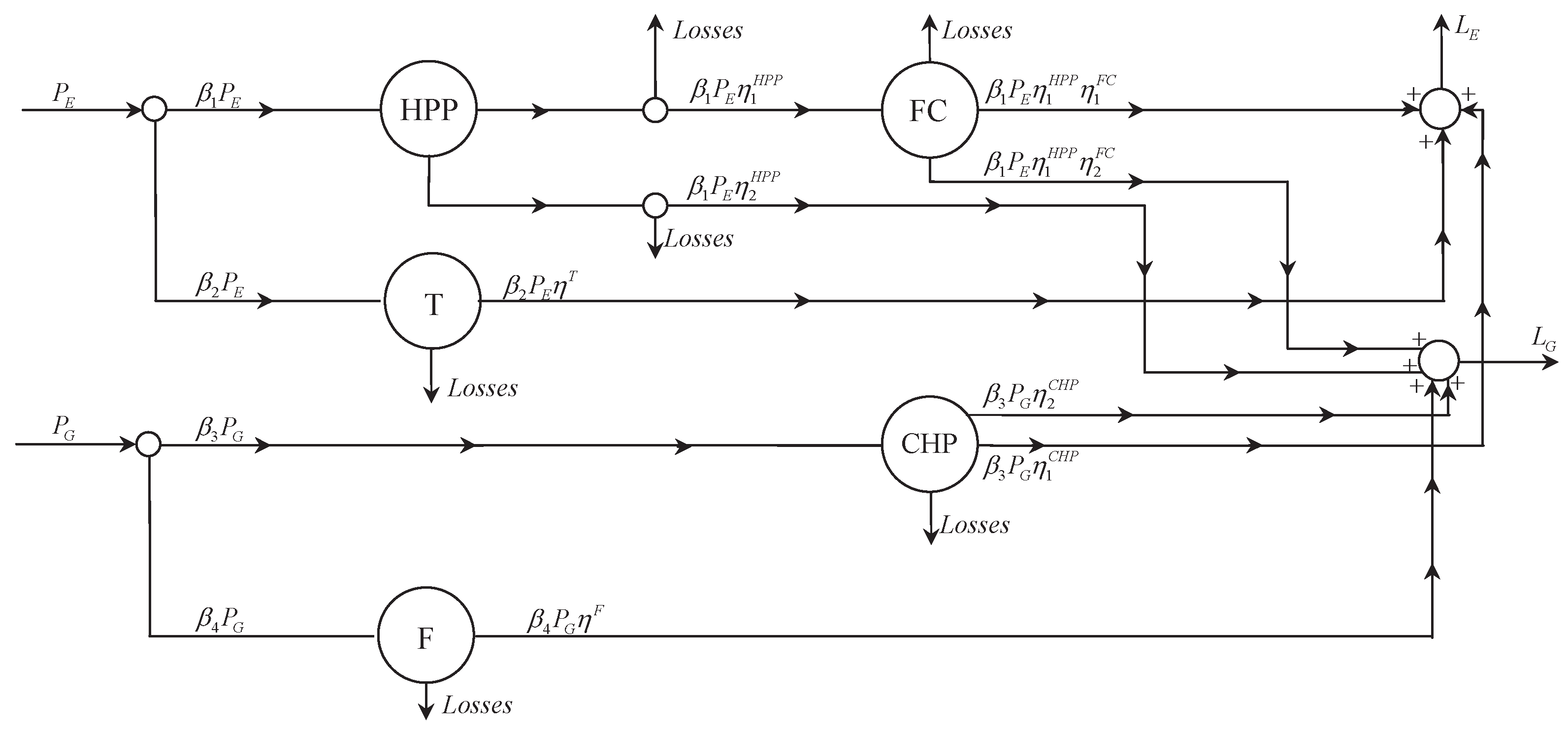
To assess the effectiveness of the proposed methodology in the task of solving real operation problems in complex networked systems, the problem of optimal energy flow management of a realistic energy hub is here considered. This is a relevant problem in modern energy systems, where the increasing inter-dependencies between heterogeneous energy infrastructures is introducing new and more complex vulnerabilities, requiring effective modeling and optimization tools aimed at improving the accuracy and the robustness of coordinated control actions. In this context, the large scale deployment for the energy hub could have a strategic role, since it allows improving the energy networks flexibility by providing reliable energy services, such as electricity and heating, by exploiting different combinations of the energy carriers available at the hub inputs. To this aim, a system designed in Waterloo, Canada, for the supply of commercial load, has been analyzed. More details on this system, which is schematically depicted in Figure 1, can be found in [11].

From Figure 1 it is worth noting as the input power flows are the electricity,

P_{E}

, and the natural gas,

P_{G}

, while the output power flows are electricity,

L_{E}

, and heat,

L_{H}

. Notice that

P_{E}

is splitted into

β_{1} P_{E}

and

β_{2} P_{E}

, while

P_{G}

is divided into

β_{3} P_{G}

and

β_{4} P_{G}

. Precisely,

β_{1} P_{E}

and

β_{2} P_{E}

are, respectively, inputs of the Hydrogen Production Plant (HPP) and of the Transformer (T);

β_{3} P_{G}

is input of the Combined Heat Power (CHP), while

β_{4} P_{G}

is input of the Furnace (F). The system works as follows:

The subsystem HPP, characterized by electric-hydrogen and heat-hydrogen efficiences $η_{1}^{H P P}$ and $η_{2}^{H P P}$ , transforms a part of the electricity, $β_{1} P_{E} η_{1}^{H P P}$ , into hydrogen that feeds the Fuel Cell (FC) and another part, $β_{1} P_{E} η_{2}^{H P P}$ , into heat.
Using the hydrogen-electricity and hydrogen-heat efficiencies $η_{1}^{F C}$ and $η_{2}^{F C}$ , the subsystem FC transform a part of the hydrogen, $β_{1} P_{E} η_{1}^{H P P} η_{1}^{F C}$ , into electricity and another part, $β_{1} P_{E} η_{1}^{H P P} η_{2}^{F C}$ , into heat.
The subsystem T, due to its efficiency $η^{T}$ , has the electricity power flow $β_{2} P_{E} η^{T}$ as output.
The subsystem CHP, considering the gas-electric and gas-heat efficiencies $η_{1}^{C H P}$ and $η_{2}^{C H P}$ , transforms a part of natural gas, $β_{3} P_{G} η_{1}^{C H P}$ , into electricity and another part, $β_{3} P_{G} η_{2}^{C H P}$ , into heat.
Finally, the subsystem F, characterized by its efficiency $η^{F}$ , has output $β_{4} P_{G} η^{F}$ , that is heat.

As for the outputs of the energy hub, we simply get that:

L_{E} = β_{1} P_{E} η_{1}^{H P P} η_{1}^{F C} + β_{2} P_{E} η^{T} + β_{3} P_{G} η_{1}^{C H P},

(7)

L_{H} = β_{1} P_{E} η_{1}^{H P P} η_{2}^{F C} + β_{1} P_{E} η_{2}^{H P P} + β_{3} P_{G} η_{2}^{C H P} + β_{4} P_{G} η^{F} .

(8)

Notice that (7) and (8) are obtained considering some losses that depend on coefficients

η_{1}^{H P P}

η_{2}^{H P P}

η_{1}^{F C}

η_{2}^{F C}

η^{T}

η_{1}^{C H P}

η_{2}^{C H P}

and

η^{F}

. Such parameters are usually fixed and, for the topology described in Figure 1, they are the following:

η_{1}^{H P P} = 0.7,

η_{2}^{H P P} = 0.2,

η_{1}^{F C} = 0.55,

η_{2}^{F C} = 0.4,

η^{T} = 0.98,

η_{1}^{C H P} = 0.45,

η_{2}^{C H P} = 0.35,

η^{F} = 0.48

. Moreover, note that

β_{2} = 1 - β_{1},

β_{4} = 1 - β_{3},

0 < β_{1} < 1,

0 < β_{2} < 1

, hence there is the possibility of choosing how to redistribute incoming flows over the energy hub.

The definition of optimal energy hub operation strategies could follow different directions. An example is described in [11]. In our case, for fixed incoming flows

P_{E}

and

P_{G}

, we want to find the optimal coefficients

β_{1}

and

β_{2}

(of nodes with one incoming arc and two outgoing ones) such that the global energy conversion losses are minimized. Obviously, different and more general operation criteria could be defined, without affecting the effectiveness of the proposed methodology.

In order to achieve this aim, we choose to model the energy hub using an approach dealing with conservation laws on networks (an exhaustive overview is in [18]), considering that eventual losses over the system are considered “output” different from

L_{E}

and

L_{H}

4.2. Numerical Results

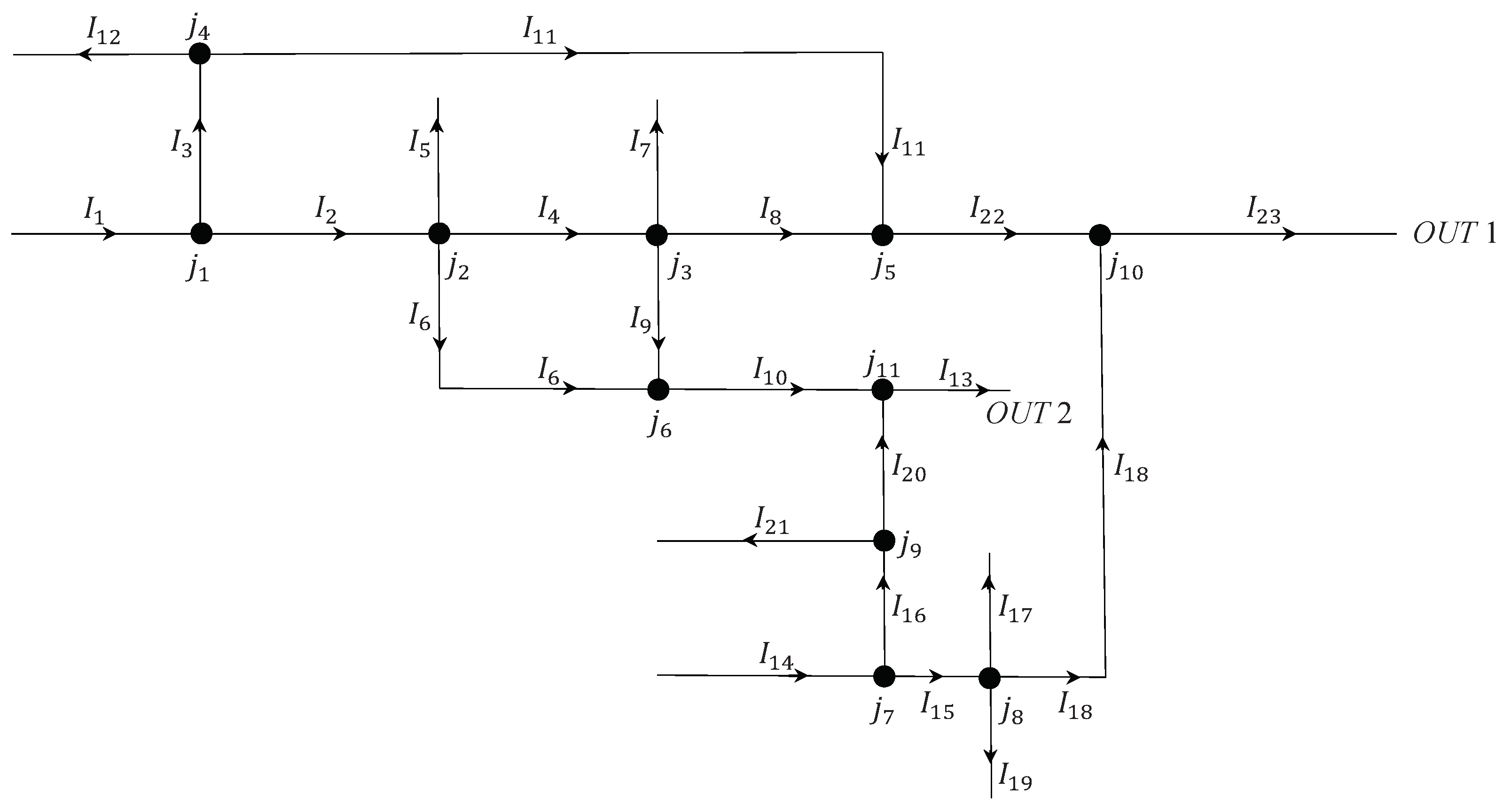
This section presents the simulations for the energy hub, represented in Figure 2 as a couple

(I, J)

, with

I = {\{I_{n}\}}_{n = 1, . ., 23}

and

J = {\{j_{k}\}}_{k = 1, . ., 11}

, see Section 2. The features of the network in Figure 2 are as follows. External arcs:

I_{1}

I_{5}

I_{7}

I_{12}

I_{13}

I_{14}

I_{17}

I_{19}

I_{21}

I_{23}

. Inner arcs:

I_{2}

I_{3}

I_{4}

I_{6}

I_{8}

I_{9}

I_{10}

I_{11}

I_{15}

I_{16}

I_{18}

I_{20}

I_{22}

. Nodes of:

1 \times 2

type,

j_{1}

j_{4}

j_{7}

j_{9}

;

2 \times 1

type:

j_{5}

j_{6}

j_{10}

j_{11}

;

1 \times 3

type:

j_{2}

j_{3}

j_{8}

For simplicity of discussion, from now on we indicate a node

j_{k}

and its distribution matrix

A_{j_{k}}

simply by k and

A_{k}

, respectively; the same with arc

I_{m}

, named simply m.

Notice that arcs 1 and 14 are the inputs of the systems, while outputs are arcs 13 and 23, indicated, respectively, by

O U T

2 and

O U T

The performances of the network are evaluated through the cost functional

\bar{E} (t)

, whose evolution is deeply influenced by the distribution parameters. Indeed, due to the real characteristics of the energy hub, for nodes 2, 3, 4, 8 and 9, distribution matrices

A_{J}

J \in \{2, 3, 4, 8, 9\}

assume the form:

A_{2} = (\begin{matrix} c α_{4, 2} \\ α_{5, 2} \\ α_{6, 2} \end{matrix}) = (\begin{matrix} c 0.7 \\ 0.1 \\ 0.2 \end{matrix}),

A_{3} = (\begin{matrix} c α_{7, 4} \\ α_{8, 4} \\ α_{9, 4} \end{matrix}) = (\begin{matrix} c 0.05 \\ 0.55 \\ 0.4 \end{matrix}),

A_{4} = (\begin{matrix} c α_{11, 3} \\ α_{12, 3} \end{matrix}) = (\begin{matrix} c 0.98 \\ 0.02 \end{matrix}),

A_{8} = (\begin{matrix} c α_{17, 15} \\ α_{18, 15} \\ α_{19, 15} \end{matrix}) = (\begin{matrix} c 0.2 \\ 0.45 \\ 0.35 \end{matrix}),

A_{9} = (\begin{matrix} c α_{20, 16} \\ α_{21, 16} \end{matrix}) = (\begin{matrix} c 0.68 \\ 0.32 \end{matrix}) .

Moreover, always referring to measures on the real hub, priority parameters are all chosen

0.5

for incoming arcs of nodes 5, 6, 10 and 11. Hence, no control is considered for junctions 2, 3, 4, 5, 6, 8, 9, 10 and 11, and the optimization of

\bar{E} (t)

deals only with the distribution coefficients at nodes 1 and 7 of

1 \times 2

type.

As for the numerical construction of

\bar{E} (t)

, it is necessary a suitable approximation for densities

ρ_{i} (t, x)

i = 1, \dots, 23

, whose evolution is ruled by equation (1).

In this paper, we apply the Godunov scheme (see [32,33,34]),using a numerical grid with constant space and time sizes,

Δ x = 0.0125

and

Δ t = 0.5 Δ x

, respectively (see subSection 4.4 for details about the computational cost). The network of Figure 2 is simulated in such conditions: time interval of simulation:

[0, T]

, with

T = 150 min

; empty arcs when the simulation starts (

t = 0

); boundary data of Dirichlet type, equal to

0.3

for arcs 1 and 14 while, for arcs 5, 7, 12, 13, 17, 19, 21 and 23, we choose a Dirichlet boundary data equal to

0.9

Notice that typical maximal values for inputs of our hub are 15 MWh and 20 MWh for arcs 1 and 14, respectively. In our case, associating at

ρ_{max} = 1

the quantity 15 MWh, we simply get that boundary data

0.3

and

0.9

correspond to

4.5

MWh and

13.5

MWh.

Two different choices of the distribution parameters are assumed for nodes 1 and 7:

optimal case: parameters that optimize locally the asymptotic behaviour of $\bar{E} (t)$ , i.e. distribution coefficients that refer to Theorem 1 for junctions 1 and 7. Such type of simulation is useful to test the global performance, starting from analytical results that consider only a part of nodes of the network.
random case: parameters at nodes 1 and 7 are chosen in a random way at $t = 0$ and then are kept constant in $[0, T]$ . A random simulation allows comparisons with network performances obtained via local optimal distribution coefficients.

4.3. Results Discussion

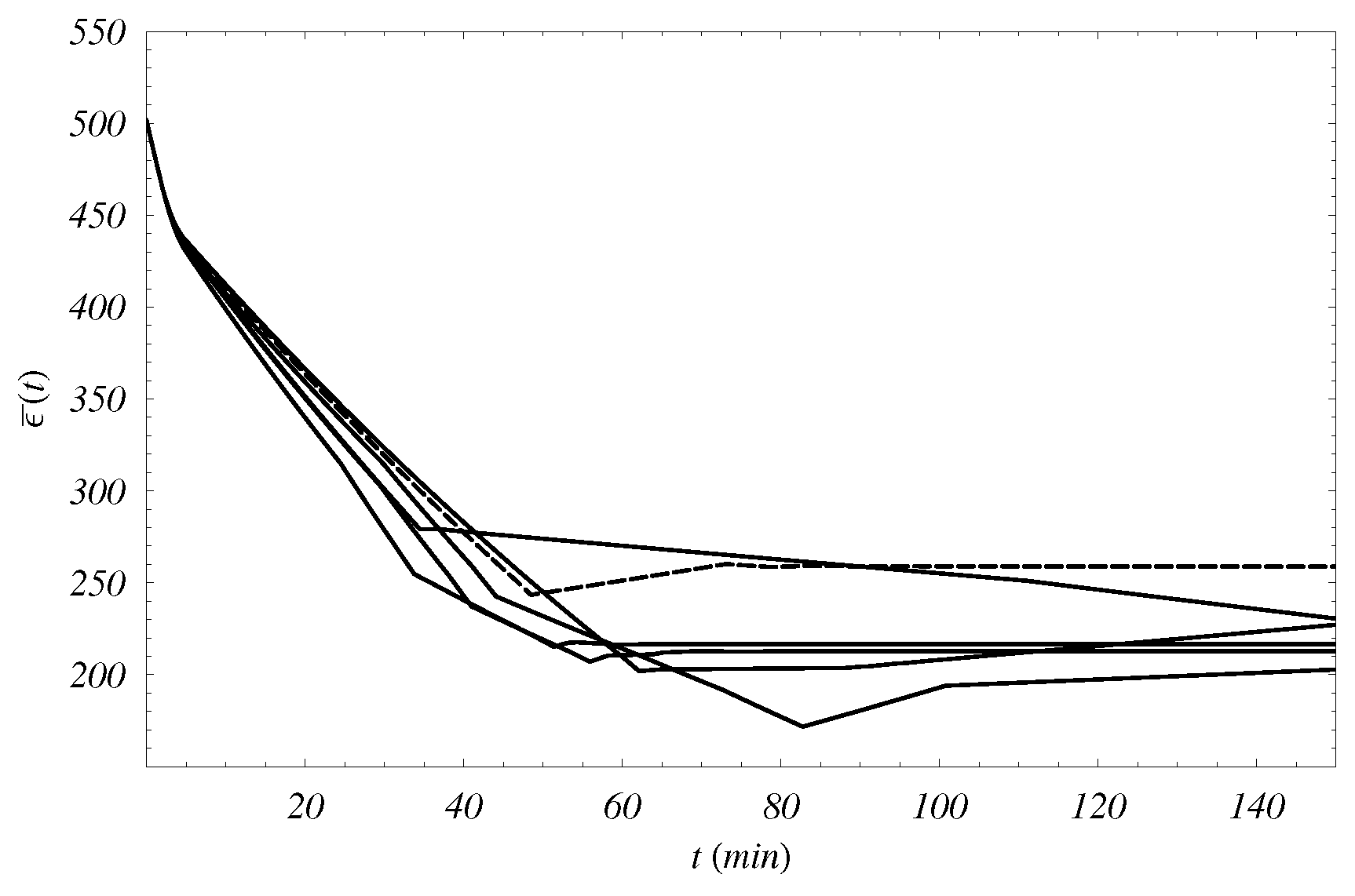
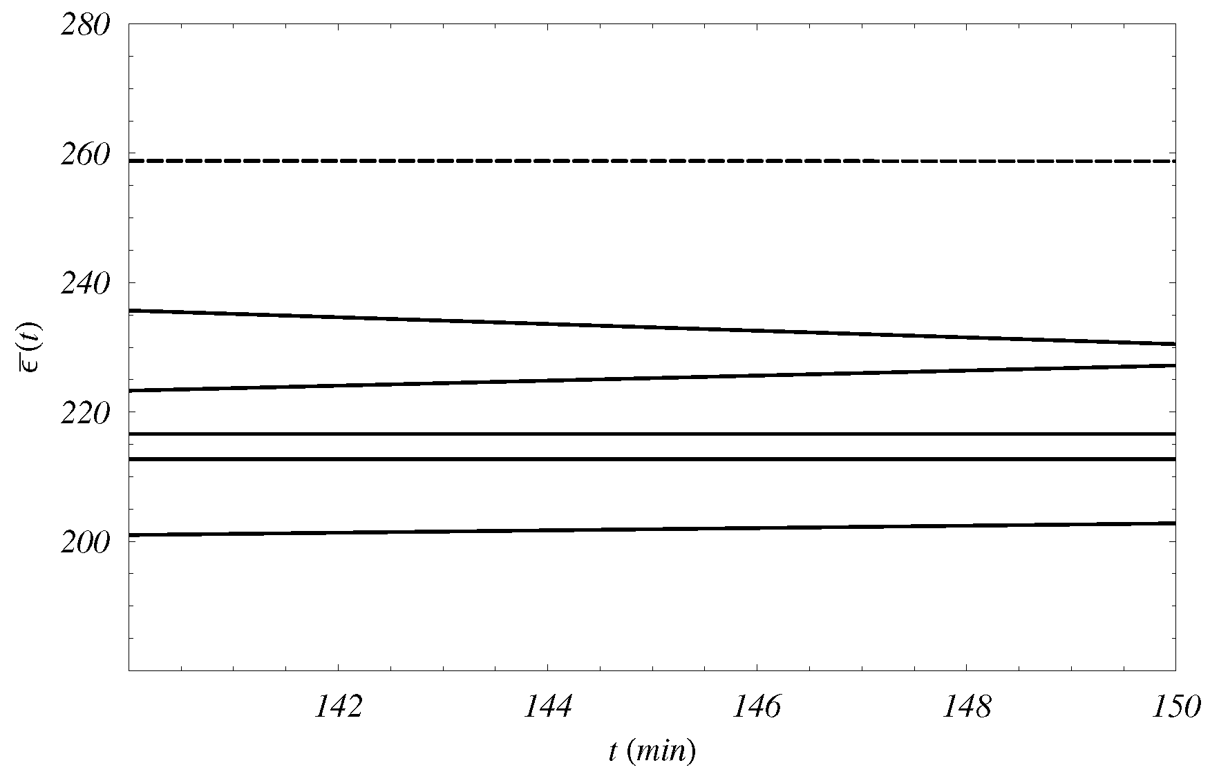
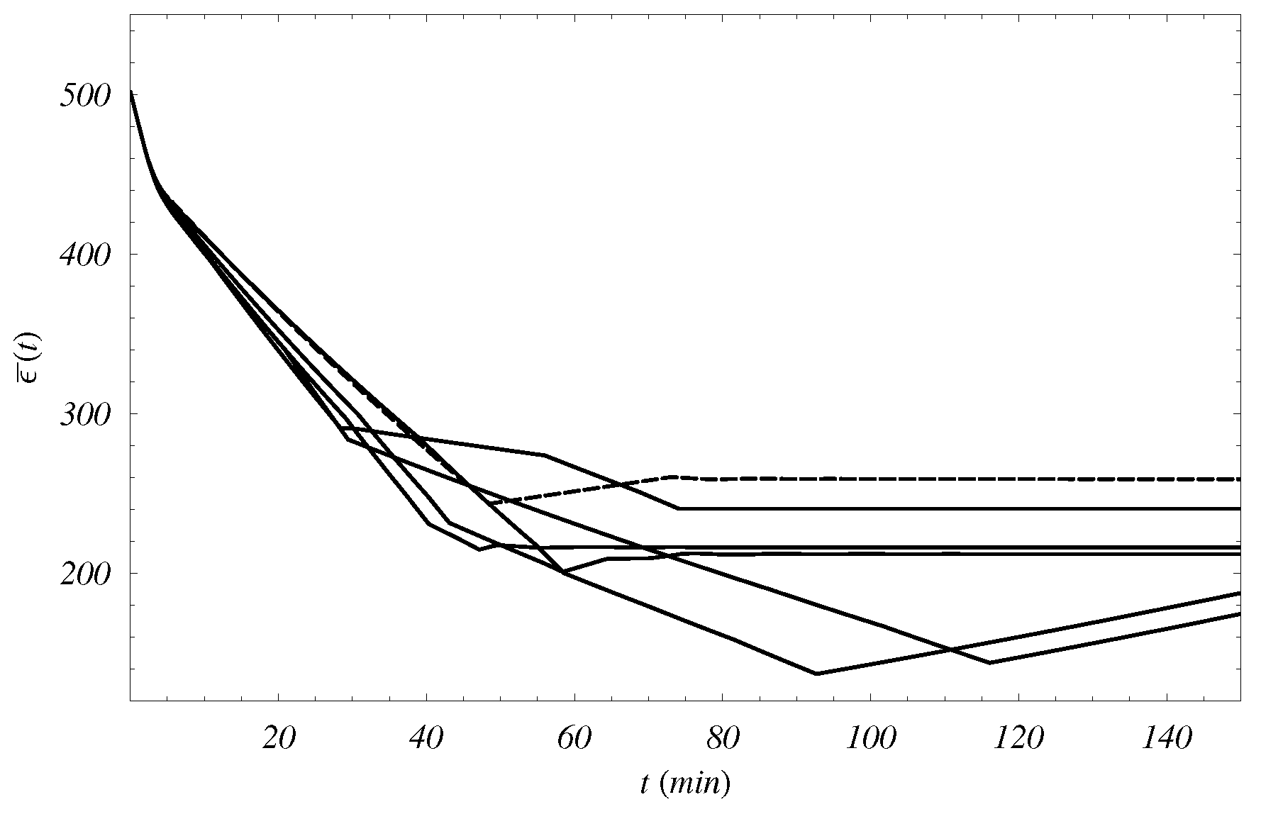
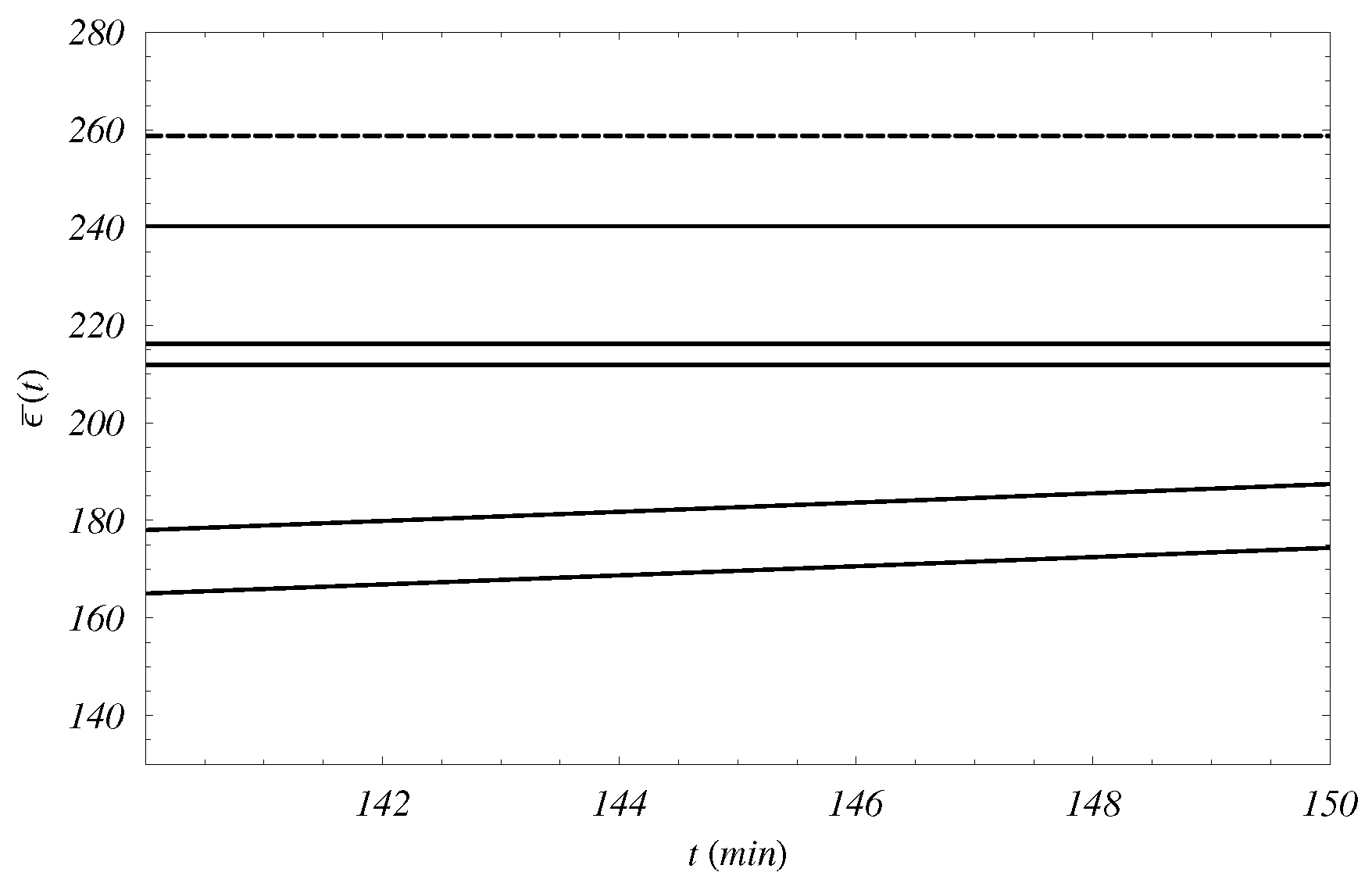
In Figure 3, Figure 4, Figure 5 and Figure 6 we show some simulation results for the energy hub. More precisely, the values of

\bar{E} (t)

, computed on the whole network, is represented as function of the time.

In particular, the behavior of

\bar{E} (t)

in the optimal case is compared with the ones obtained via ten different simulation random studies. As for these last cases, Figure 3 and Figure 4 show the first five ones, while Figure 5 and Figure 6 the remaining other ones.

The optimization algorithm for

1 \times 2

nodes, which is of local type, can be applied to the complex topology of the energy hub without compromising the possibility of a global optimization. Such a situation is evident in the optimal case for

\bar{E} (t)

, that is compared to the behaviors in ten different random cases. In Figure 3, Figure 4, Figure 5 and Figure 6, it is shown that the optimal case is always higher than random cases.

Indeed, 100 random cases have been simulated and compared with the optimal behavior for

\bar{E} (t)

. Table 1 reports the value of

\bar{E} (t)

in the optimal configuration at

T = 150

, i.e. OPTconf T, with the average value (RAND T) of random simulations at

T = 150

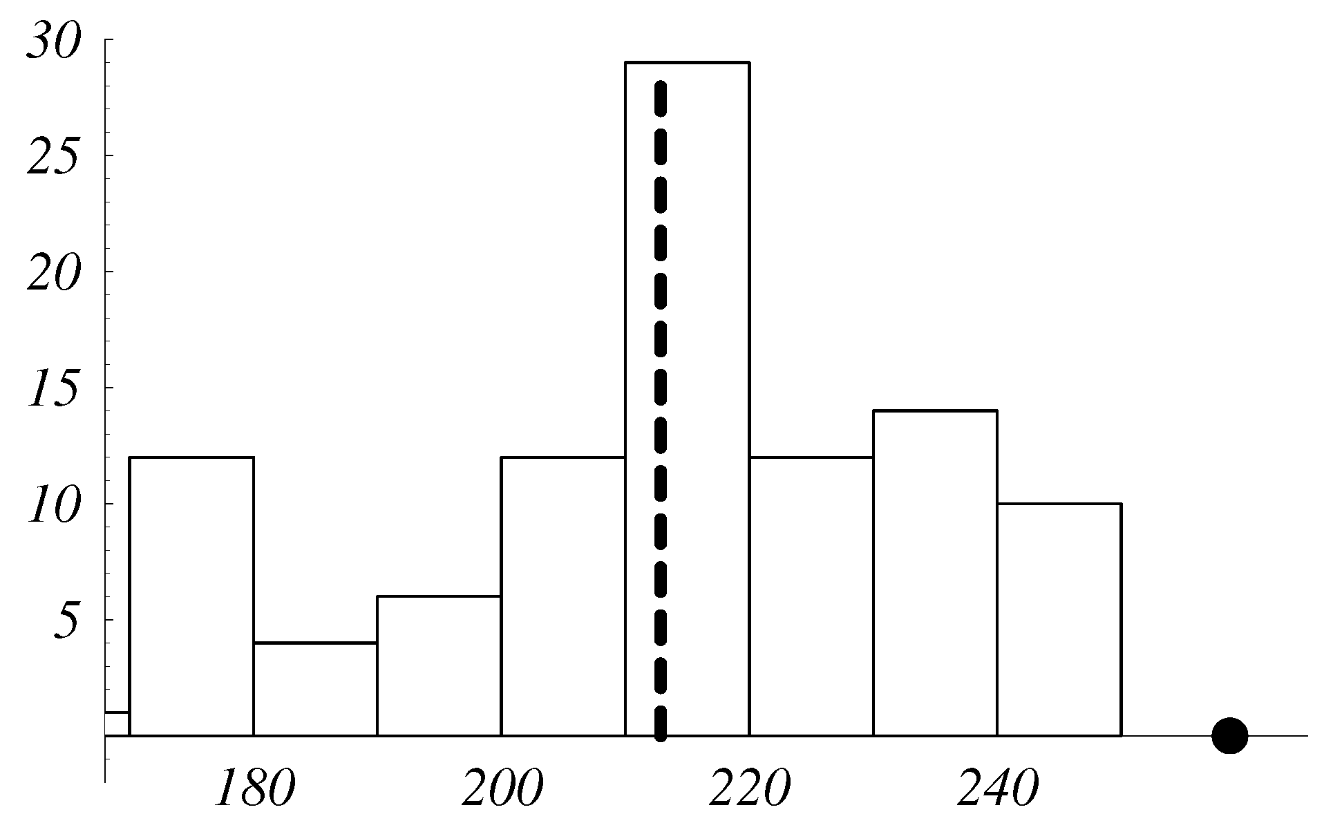
Notice that OPTconf T is, as expected, higher than RAND T, namely the global optimization of local type has a strong robustness. Such result is also represented in Figure 7, where a histogram reports the values of

\bar{E} (t)

at the final instant T for the random simulation.

Finally, notice that the simulated system has always bounded outputs, as a consequence of the model itself, which deals with limited densities on arcs (see Section 2). In particular, in our case study, the upper limits for arcs 13 and 23 (

O U T

2 and

O U T

1) are, respectively,

0.1218

(

36.54

kWh) and

0.180075

(

54.0225

kWh).

4.4. Computational Cost

This subsection presents some details about the computational cost for the simulation of the presented energy system. Focus on a network represented by the couple

(I, J)

, with

I = {\{I_{n}\}}_{n = 1, . ., N}

and

J = {\{j_{k}\}}_{k = 1, . ., J}

In order to find a suitable numerical approximation in

[0, T]

for the density functions

ρ_{n} (t, x)

n = 1, . ., N

, on arcs and update of boundary data at nodes, assume that each arc

I_{n}

n = 1, . ., N

, has length

L_{n}

; space and time grid sizes are, respectively,

Δ x_{n}

and

Δ t_{n}

. Using the Godunov method, the computational cost depends on

\sum_{n = 1}^{N} \frac{L_{n}}{Δ x_{n}}

and

\sum_{k = 1}^{J} \frac{T}{Δ t_{k}}

for densities and boundary data, respectively.

For simplicity, for the simulation of the described energy hub we consider a constant space grid size

Δ x

, assume

(Δ x_{n}, Δ t_{n}) = (Δ x, 0.5 Δ x)

∀

n = 1, \dots, N

, and compute the CPU times (measured in seconds and calculated by an Intel(R) Core (TM) i7-3630 QM CPU @2.40 GHz, RAM 8 GB) and convergence errors. The obtained results are in Table 2.

From the previous table, we simply get that the CPU time increases of about 0.30 seconds when

Δ x

decreases. As for the convergence error, it almost remains the same for different values of

Δ x

. Some further studies, as well as different numerical approaches for conservation laws on networks, are carefully analyzed in [18,23] and [30].

5. Conclusions

In this paper the theoretical foundations of a novel computing paradigm based on the fluid dynamic theory for modeling, analysis and optimization of complex and networked energy systems have been presented. The proposed paradigm is based on the challenging idea of integrating in a unique framework both network modeling and the optimization features, which are traditionally treated as two separate problems, and solved by using distinct solution techniques. To address this issue the application of conservation laws and the definition of cost functional, which represents a term proportional to the kinetic energy of the system, have been proposed for dealing with the network modeling and optimization, respectively. Thanks to these features the functional maximization is directly obtained as a result of the network model process, which optimally tunes the network parameters ruling the distribution of the energy flows among the network arcs.

The benefits due to the application of the proposed approach have been assessed on a realistic case study, dealing with the solution of the optimal energy flow management problem for a complex energy hub designed in Waterloo, Canada. The obtained results demonstrated the effectiveness of the fluid dynamic-based approach in the task of optimizing the energy flows of the hub components in order to drastically reduce the conversion losses.

Finally, on the basis of repetitive simulations, it could be argue that the obtained solution is globally optimal, and robust against distributed parameters variations, which can be considered further, and certainly relevant, benefits. A rigorous theoretical justification of these intuitions are currently under investigation by the authors.

Author Contributions

Conceptualization, M.d.F. and A.V.; methodology, L.R. and A.V.; software, L.R.; validation, M.d.F., L.R. and A.V.; formal analysis, L.R. and A.V.; investigation, L.R. and A.V.; writing—original draft preparation, M.d.F., L.R. and A.V.; writing—review and editing, L.R. and A.V.; supervision, M.d.F., L.R. and A.V.; project administration, M.d.F., L.R. and A.V. All authors have read and agreed to the published version of the manuscript.

Funding

This research received no external funding.

Data Availability Statement

Not applicable.

Conflicts of Interest

The authors declare no conflicts of interest.

Appendix A

Following rules (A) and (B) and adopting the flux function (2), see Section 2, we provide precise details for the construction of

ρ_{i}^{k} (t, x)

for a node

j_{k} \in J

r \times s

type with distribution matrix

A_{j_{k}}

. The basic step is to find the solution to the RP at

j_{k}

, namely the vector

{\hat{γ}}^{k} = f ({\hat{ρ}}^{k}) \in {[0, \frac{ρ_{max}}{2}]}^{r + s}

, that is:

{\hat{γ}}^{k} : = ({\hat{γ}}_{1}^{k}, {\hat{γ}}_{2}^{k}, \dots, {\hat{γ}}_{r}^{k}, {\hat{γ}}_{r + 1}^{k}, {\hat{γ}}_{r + 2}^{k}, \dots, {\hat{γ}}_{r + s}^{k}) .

The solution to the RP at

j_{k}

on the incoming arcs is indicated by the first r components of

{\hat{γ}}^{k}

, i.e.

{\hat{γ}}_{i n}^{k} : = ({\hat{γ}}_{1}^{k}, {\hat{γ}}_{2}^{k}, \dots, {\hat{γ}}_{r}^{k}) \in {[0, \frac{ρ_{max}}{2}]}^{r}

; the last s components of

{\hat{γ}}^{k}

, represented by

{\hat{γ}}_{o u t}^{k} : = ({\hat{γ}}_{r + 1}^{k}, {\hat{γ}}_{r + 2}^{k}, \dots, {\hat{γ}}_{r + s}^{k}) \in {[0, \frac{ρ_{max}}{2}]}^{s}

, refer to the solution to the RP at

j_{k}

for the outgoing arcs.

From rule (A), we simply get:

{({\hat{γ}}_{o u t}^{k})}^{T} = A_{j_{k}} \cdot {({\hat{γ}}_{i n}^{k})}^{T} .

(A1)

Rule (B) defines

{\hat{γ}}_{i n}^{k}

that, in case

γ : = (γ_{1}, γ_{2}, \dots, γ_{r}) \in R^{r}

, is solution of the linear programming problem

P_{j_{k}}

(P_{j_{k}}) max_{γ} \sum_{φ = 1}^{r} γ_{φ},

(A2)

with constraints:

γ \in \prod_{φ = 1}^{r} [0, γ_{φ}^{k, max}], A_{j_{k}} \cdot γ^{T} \in \prod_{ψ = r + 1}^{r + s} [0, γ_{ψ}^{k, max}] .

Finally, the solution

ρ^{k} (t, x) = (ρ_{1}^{k} (t, x), \dots, ρ_{r}^{k} (t, x), ρ_{r + 1}^{k} (t, x), \dots, ρ_{r + s}^{k} (t, x)) \in {[0, ρ_{max}]}^{r + s}

j_{k}

is obtained as follows.

(S1) From (9) and (10), find ${\hat{γ}}^{k}$ .
(S2) Use definitions for ${\hat{ρ}}_{φ}^{k}$ and ${\hat{ρ}}_{ψ}^{k}$ , see Section 2, to get ${\hat{ρ}}^{k}$ . Precisely, for the incoming arc $I_{φ}^{k}$ , $φ = 1, \dots, r$ :

${\hat{ρ}}_{φ}^{k} = \{\begin{matrix} ρ_{φ, 0}^{k}, & if 0 \leq ρ_{φ, 0}^{k} \leq \frac{ρ_{max}}{2} and {\hat{γ}}_{φ}^{k} = γ_{φ}^{k, max}, \\ \frac{v_{max} ρ_{max} + \sqrt{v_{max} ρ_{max} (v_{max} ρ_{max} - 4 {\hat{γ}}_{φ}^{k})}}{2 v_{max}}, & \begin{matrix} if 0 \leq ρ_{φ, 0}^{k} \leq \frac{ρ_{max}}{2} and {\hat{γ}}_{φ}^{k} < γ_{φ}^{k, max}, \end{matrix} \\ or \frac{ρ_{max}}{2} \leq ρ_{φ, 0}^{k} \leq ρ_{max} . \end{matrix}$

For the outgoing arc $I_{ψ}^{k}$ , $ψ = r + 1, \dots, r + s$ :

${\hat{ρ}}_{ψ}^{k} = \{\begin{cases} \frac{v_{max} ρ_{max} - \sqrt{v_{max} ρ_{max} (v_{max} ρ_{max} - 4 {\hat{γ}}_{ψ}^{k})}}{2 v_{max}}, & if 0 \leq ρ_{ψ, 0}^{k} \leq \frac{ρ_{max}}{2}, \\ or if \frac{ρ_{max}}{2} \leq ρ_{ψ, 0}^{k} \leq ρ_{max} and {\hat{γ}}_{ψ}^{k} < γ_{ψ}^{k, max}, \\ ρ_{ψ, 0}^{k}, & if \frac{ρ_{max}}{2} \leq ρ_{ψ, 0}^{k} \leq ρ_{max} and {\hat{γ}}_{ψ}^{k} = γ_{ψ}^{k, max}; \end{cases}$
(S3) For each arc $I_{i}^{k}$ , $i = 1, \dots, r + s$ , solve the initial-boundary value problem:

$\{\begin{matrix} {(ρ_{i}^{k})}_{t} + f {(ρ_{i}^{k})}_{x} = 0, x \in I_{i}^{k}, t > 0, \\ ρ_{i}^{k} (0, x) = ρ_{i, 0}^{k}, \\ ρ_{i}^{k} (t, 0) = {\hat{ρ}}_{i}^{k} . \end{matrix}$

References

Abdeltawab, H.H.; Mohamed, Y. A. R. I. Market-Oriented Energy Management of a Hybrid Wind-Battery Energy Storage System Via Model Predictive Control With Constraint Optimizer, IEEE Transactions on Industrial Electronics, 2015, 62(11), 6658–6670. [CrossRef]
Jarden, R. K.; Stumpf, P.; Varga, Z.; Nagy, I. Novel Solutions for High-Speed Self-Excited Induction Generators, IEEE Transactions on Industrial Electronics, 2016, 63(4), 2124–2132. [CrossRef]
Arefifar, S.A.; Mohamed, Y. A. I. Probabilistic Optimal Reactive Power Planning in Distribution Systems with Renewable Resources in Grid-Connected and Islanded Modes, IEEE Transactions on Industrial Electronics, 2014, 61(11), 5830–5839. [CrossRef]
Blaabjerg, F.; Teodorescu, R.; Liserre, M.; Timbus, A. V. Overview and Control and Grid Synchronization for Distributed Power Generation Systems, IEEE Transactions on Industrial Electronics, 2006, 53(5), 1398–1409. [CrossRef]
Carrasco, J.M.; Franquelo, L. G.; Bialasiawicz, J. T.; Galván, E., Portillo Guisardo, R. C.; Prats, M. Á. M.; León, J. I.; Moreno-Alfonso, N. Power-Electronic Systems for the Grid Integration of Renewable Energy Sources: A Survey, IEEE Transactions on Industrial Electronics, 2006, 53(4), 1002–1016. [CrossRef]
Gaeta, M.; Loia, V.; Tomasiello, S. Multisignal 1D-compression by F-transform for wireless sensor networks, Applied Soft Computing, 2015, 30, 329–340. [CrossRef]
Tomasiello, S. Least–Squares Fuzzy Transforms and Autoencoders: Some Remarks and Application, IEEE Transactions on Fuzzy Systems, 2021, 29(1), 129–136. [CrossRef]
Chicco, G.; Mancarella, P. Distributed multi-generation: a comprehensive view, Renew Sustain Energy Rev, 2009, 13, 535—555. [CrossRef]
Geidls, M.; Koeppel, G.; Favre-Perrod, P.; Klöckl, B.; Andersson, G.; Fröhlich, K. Energy hubs for the future, IEEE Power Energy Mag, 2007, 5, 24—30. [CrossRef]
Krause, T.; Andersson, G.; Fröhlich, K.; Vaccaro, A., Multiple-energy carriers: modeling of production delivery and consumption, Proc IEEE 2011, 2011, 99(1), 15—27. [CrossRef]
Parisio, A.; Del Vecchio, C.; Vaccaro, A. A robust optimization approach to energy hub management, Electrical Power and Energy Systems, 2012, 42, 98—104. [CrossRef]
Schulze, M.; Friedrich, L.; Gautschi, M. Modeling and optimization of renewables: applying the energy hub approach, 2008, Proceedings of IEEE International Conference on Sustainable Energy Technologies, 83–88. [CrossRef]
Bertsimas, D.; Sim, M. The price of robustness, Oper Res, 2004, 54(1), 35–53. [CrossRef]
Bressan, A. Hyperbolic Systems of Conservation Laws - The One - dimensional Cauchy Problem; Oxford University Press, 2000.
Lighthill, M. J.; Whitham, G. B. On kinetic waves. II. Theory of Traffic Flows on Long Crowded arcs, Proc. Roy. Soc. London Ser. A, 1955, 229, 317–345. [CrossRef]
Richards, P. I. Shock Waves on the Highway, Oper. Res., 1956, 4, 42–51. [CrossRef]
Coclite, G.; Garavello, M.; Piccoli, B. Traffic Flow on road Networks, SIAM Journal on Mathematical Analysis, 2005, 36, 1862–1886. [CrossRef]
Garavello, M.; Piccoli, B. Traffic Flow on Networks, Applied Math Series Vol. 1, American Institute of Mathematical Sciences, 2006.
Holden, H.; Risebro, N. H. A Mathematical Model of Traffic Flow on a Network of Unidirectional arcs, SIAM J. Math. Anal., 1995, 26, 999–1017. [CrossRef]
Kupenko, O. P.; Manzo, R. Approximation of an optimal control problem in coefficient for variational inequality with anisotropic p-Laplacian, Nonlinear Differential Equations and Applications, 2016, 23(31), Article number 35. [CrossRef]
Kupenko, O. P.; Manzo, R. On optimal controls in coefficients for ill-posed non-linear elliptic dirichlet boundary value problems, Discrete and Continuous Dynamical Systems - Series B, 2018, 23(4), 1363–1393. [CrossRef]
Jiang, T.; Zhang, C.; Zhu, H.; Gu, J.; Deng, G. Energy-Efficient Scheduling for a Job Shop Using an Improved Whale Optimization Algorithm, Mathematics, 2018, 6(11), 220. [CrossRef]
Cutolo, A.; Piccoli, B.; Rarità, L. An Upwind-Euler scheme for an ODE-PDE model of supply chains, SIAM Journal on Computing, 2011, 33(4), 1669–1688. [CrossRef]
Helbing, D.; Lämmer, S.; Lebacque, J. P. Self-organized control of irregular or perturbed network traffic, Optimal Control and Dynamic Games, C. Deissenberg and R. F. Hartl eds., Springer, Dordrecht, 2005, 239–274. [CrossRef]
Herty, M.; Klar, A. Modelling, Simulation and Optimization of Traffic Flow Networks, SIAM J. Sci. Comp., 2003, 25, 1066–1087. [CrossRef]
Rarità, L., A genetic algorithm to optimize dynamics of supply chains, L. Amorosi et al. (eds) Optimization in Artifical Intelligence and Data Sciences. AIRO Springer Series 8, 2022, 107-115. [CrossRef]
Rarità, L.; Stamova, I.; Tomasiello, S. Numerical schemes and genetic algorithms for the optimal control of a continuous model of supply chains, Applied Mathematics and Computation, 2021, 388, 125464. [CrossRef]
Zhang, Z.; Wu, Z.; Raicon, D.; Christofides, P. D. Real-Time Optimization and Control of Nonlinear Processes Using Machine Learning, Mathematics, 2019, 7(10), 890. [CrossRef]
Garavello, M.; Piccoli, B. Traffic flow on a road network using the Aw-Rascle model, Commun. Partial Diff. Eqns., 2006, 31, 243–275. [CrossRef]
Bretti, G.; Natalini, R.; Piccoli, B. Numerical approximations of a traffic flow model on networks, Networks and Heterogeneous Media, 2006, 1(1), 57–84. [CrossRef]
Cascone, A.; Marigo, A.; Piccoli, B.; Rarità, L. Decentralized optimal routing for packets flow on data networks, Discrete and Continuous Dynamical Systems, Series B, 2010, 13(1), 59–78. [CrossRef]
Godlewsky, E.; Raviart, P. Numerical Approximation of Hyperbolic Systems of Conservation Laws, Springer Verlag, Heidelberg, 1996.
Godunov, S. K. A finite difference method for the numerical computation of discontinuous solutions of the equations of fluid dynamics, Mat. Sb., 1959, 47, 271–306.
Lebacque, J. P.; Lesort, J. B. The Godunov scheme and what it means for first order traffic flow models, Proceedings of the Internaional symposium on transportation and traffic theory No13, Lyon, Pergamon Press, Oxford, 1996, 647–677.

Figure 1. Simplified structure of the energy hub shown in [11].

Figure 2. Topology of the energy hub.

Figure 3. Evolution in

[0, T]

\bar{E} (t)

for optimal distribution coefficients (dashed line) and the first five different random choices (continuous lines).

Figure 3. Evolution in

[0, T]

\bar{E} (t)

for optimal distribution coefficients (dashed line) and the first five different random choices (continuous lines).

Figure 4. Zoom of Figure 3 around the asymptotic values.

Figure 5. Behaviour in

[0, T]

\bar{E} (t)

in case of optimal distribution coefficients (dashed line) and the remaining different random choices (continuous lines).

Figure 5. Behaviour in

[0, T]

\bar{E} (t)

in case of optimal distribution coefficients (dashed line) and the remaining different random choices (continuous lines).

Figure 6. Zoom of Figure 5 around the asymptotic values.

Figure 7. Histograms of random values of simulations at

T = 150

for

[0, T]

\bar{E} (t)

. Black point: OPTconf

T = 150

; dashed line: RAND

T = 150

Figure 7. Histograms of random values of simulations at

T = 150

for

[0, T]

\bar{E} (t)

. Black point: OPTconf

T = 150

; dashed line: RAND

T = 150

Table 1. Compared values of

\bar{E} (t)

Table 1. Compared values of

\bar{E} (t)

	$\bar{E} (t)$
OPTconf T	$258.773$
RAND T	$212.845$

Table 2. CPU times and convergence order (

γ

)

Table 2. CPU times and convergence order (

γ

)

Space grid size	$Δ x = 0.00625$	$Δ x = 0.0125$	$Δ x = 0.025$
CPU and convergence order	CPU $= 0.97$ $γ = 0.96653$	CPU $= 0.62$ $γ = 0.92572$	CPU $= 0.33$ $γ = 0.90572$

Disclaimer/Publisher’s Note: The statements, opinions and data contained in all publications are solely those of the individual author(s) and contributor(s) and not of MDPI and/or the editor(s). MDPI and/or the editor(s) disclaim responsibility for any injury to people or property resulting from any ideas, methods, instructions or products referred to in the content.

© 2024 by the authors. Licensee MDPI, Basel, Switzerland. This article is an open access article distributed under the terms and conditions of the Creative Commons Attribution (CC BY) license (http://creativecommons.org/licenses/by/4.0/).

Copyright: This open access article is published under a Creative Commons CC BY 4.0 license, which permit the free download, distribution, and reuse, provided that the author and preprint are cited in any reuse.

MDPI Initiatives

Important Links

Choose an area of interest and we will send you notifications of new preprints at your preferred frequency.

Disclaimer

A Fluid Dynamic Approach To Model And Optimize Energy Flows In Networked Systems

Abstract

1. Introduction

2. Theoretical Foundations

3. Energy Optimization

4. Application Deployment

4.1. Energy Hub Operation Scheduling

4.2. Numerical Results

4.3. Results Discussion

4.4. Computational Cost

5. Conclusions

Author Contributions

Funding

Data Availability Statement

Conflicts of Interest

Appendix A

References

MDPI Initiatives

Important Links

Subscribe