Preprint
Article

Relative Importance of Carbon Dioxide and Water in the Greenhouse Effect: Does the Tail Wag the Dog?

Altmetrics

Downloads

509

Views

1191

Comments

2

This version is not peer-reviewed

Submitted:

03 April 2024

Posted:

04 April 2024

You are already at the latest version

Alerts
Abstract
Using a detailed atmospheric radiative transfer model, we derive macroscopic relationships of downwelling and outgoing longwave radiation, useful for hydrological practice. We validate them using empirical formulae based on downwelling radiation data, which are in common use in hydrology, as well as satellite data for the outgoing radiation. We use the macroscopic relationships to infer the relative importance of carbon dioxide and water vapour in the greenhouse effect. The results show that the contribution of the former is 4% – 5%, while water and clouds dominate with a contribution of 87% – 95%. The minor effect of carbon dioxide is also confirmed by the small, non-discernible effect of the recent escalation of atmospheric CO2 concentration from 300 to 420 ppm, which is quantified at 0.5% for both downwelling and outgoing radiation. Water and clouds also perform other important functions in climate, such as regulating the heat storage and the albedo, as well as cooling the Earth’s surface though latent heat transfer, with a contribution of 50%. By confirming the major role of water on climate, these results suggest that hydrology should have a more prominent and more active role in climate research.
Keywords: 
Subject: Environmental and Earth Sciences  -   Other
A good rule of thumb to keep in mind is that anything that calls itself 'science' probably isn't.
J.R. Searle [1]

1. Introduction

A notable feature of the current period is that the classical value of science as the pursuit of the truth, independently of other interests, is gradually being abandoned [2]. People pride themselves on being scientists and (political) activists at the same time [3], while calls for political actions to “save the planet”, including enhanced global governance mechanisms, are published even in scientific journals (e.g. [4]). A relevant example is provided by the high-profile journal Nature, which declares that it is “committed to supporting the research enterprise” [5], but admits being involved in politics and proclaims that this is the right thing [6,7], even though it is recognized that this affects scientific credibility and causes loss of confidence in science [8,9]. It is thus natural to wonder if articles published in scientific journals promote the truth or political aims, perhaps hiding or distorting the truth, and even reversing cause and effect [10,11,12,13].
Seeking truth may have been even more difficult due to a recent development, the appearance of artificial intelligence (AI) bots, which certainly affects common opinion, as well as scientific perception and advancement. Assuming that AI bots more or less reflect the common perception in the scientific community and the general public, the Microsoft Bing’s Chat bot was asked the following question:
Which gas determines the greenhouse effect on Earth?
The bot provided the following answer (also supporting it with references [14,15,16]):
The greenhouse effect is the process through which heat is trapped near Earth’s surface by substances known as ‘greenhouse gases.’ These gases consist of carbon dioxide, methane, ozone, nitrous oxide, chlorofluorocarbons, and water vapor. Water vapor, which reacts to temperature changes, is referred to as a ‘feedback’, because it amplifies the effect of forces that initially caused the warming. Scientists have determined that carbon dioxide plays a crucial role in maintaining the stability of Earth’s atmosphere. If carbon dioxide were removed, the terrestrial greenhouse effect would collapse, and Earth’s surface temperature would drop significantly, by approximately 33°C (59°F).
A literature search reveals that the AI bot essentially (and selectively) reproduces the following statements by Lacis et al. [17]:
Noncondensing greenhouse gases, which account for 25% of the total terrestrial greenhouse effect, thus serve to provide the stable temperature structure that sustains the current levels of atmospheric water vapor and clouds via feedback processes that account for the remaining 75% of the greenhouse effect. Without the radiative forcing supplied by CO₂ and the other noncondensing greenhouse gases, the terrestrial greenhouse would collapse, plunging the global climate into an icebound Earth state. […]
If the global atmospheric temperatures were to fall to as low as TS = TE [where TE = 255 K is the global mean effective temperature] the Clausius-Clapeyron relation would imply that the sustainable amount of atmospheric water vapor would become less than 10% of the current atmospheric value.
On the other hand, Koutsoyiannis and Vournas [18] recently examined longwave radiation observations extending over a period of 100 years and found that the observed increase of the atmospheric dioxide concentration ([CO₂]; from 300 to 420 ppm) has not altered, in a discernible manner, the greenhouse effect, which remains dominated by the quantity of water vapour in the atmosphere. Naturally, given the uproar about the enhancement of greenhouse effect due to human emissions by fossil fuel combustion, this finding appeared surprising to many. Some (including a knowledgeable reviewer of [18]) postulated that this would be expected for the downwelling longwave (LW) radiation flux, which was the subject of Koutsoyiannis and Vournas [18], but would not be the case for the outgoing radiation, where the effect of [CO₂] increase would be substantial. However, no long data series exist to verify such a conjecture and hence this question was not investigated in [18], whose scope was to make inference based on data.
Hence the following research questions are raised:
  • Are Lacis et al. (and the bot) right about the importance of CO₂ in the greenhouse effect, and is it meaningful to state that without it the terrestrial greenhouse would collapse? Or is the effect of CO₂ negligible as Koutsoyiannis and Vournas [18] claimed, and that of H₂O dominant?
  • Is the role of H₂O as a greenhouse gas limited to the downwelling LW flux or does it extend also to the outgoing LW flux?
We will examine these questions below, noting that the first one refers to a fictitious case (removal of atmospheric CO₂) for which no empirical data can exist. Rather, paleoclimatic studies and geological facts suggest that CO₂ existed, mostly in much higher concentrations than today, in most periods of Earth’s history, and also before oxygen appeared in the atmosphere. Also, the second question cannot be studied on an empirical basis, as no long-term data exist (systematic satellite measurements of outgoing LW flux have only been made in the 21st century). Therefore, to study these questions we need to resort to theoretical arguments and analyses. We will do this by applying the established greenhouse theory and by enrolling standard models, without considering doubts that have been cast on the validity of the theory or alternative hypotheses (e.g. [19,20]).
Human CO₂ emissions are 4% of the total [13] but there are also human H₂O emissions over the terrestrial part of Earth of a comparable percentage [21]. Specifically, according to Koutsoyiannis [22] the quantity of evaporation and transpiration over land is 91 400 km3/year. According to Food and Agriculture Organization of the United Nations [23], the human water withdrawal in 2010, including the evaporation from reservoirs, was 4.3 km3/year, of which 69% and 19% were for agricultural and industrial use, respectively. Considering the fact that almost all of agricultural and a large part of industrial water are evaporated, as well as the increasing trend in water withdrawal, with simple calculations we may conclude that the current human addition to natural water cycle over land is about 4%. One could speculate that each of these 4% additions might influence climate to a degree comparable to that percentage, but the reasons that only the influence of CO₂ is investigated and highlighted by the scientific community, being regarded a driver of climate, despite the fact that H₂O is much stronger as a greenhouse gas, should be non-scientific.
We may note, though, that this percentage becomes lower, of the order of 1%, if we also consider the evaporation over oceans. However, it appears reasonable for this estimate of human water emissions to consider only the terrestrial part of Earth, because of the high local variability and the small residence time of atmospheric water. Indeed, the mean residence time of atmospheric water is a few days (specifically, 12 250 km3 / (522 700 km3/year) = 0.23 years = 6.6 d, where the total volume of liquid water in the atmosphere, 12 250 km3, was taken as the average atmospheric water content, 24.0 kg/m3, as estimated from the ERA5 Reanalysis over the globe for the period 1950-2023, while the atmospheric inflow volume of water, 522 700 km3/year, was taken from [22]). In contrast, CO₂ is well mixed as it has a much higher residence time, of a few years (specifically, 870 Gt / (226.9 Gt/year) = 3.8 years, where the total mass of atmospheric CO₂, 870 Gt was taken from the Intergovernmental Panel on Climate Change (IPCC) report [24], namely its figure 5.12, while the atmospheric inflow mass, 226.9 Gt/year, was taken from [13]).
The thesis expressed in this paper is that none of these anthropogenic additions to hydrological and carbon cycle drives climate. On the other hand, both H₂O and CO₂ are important elements of climate and their quantities and fluxes are determined by natural processes, with the human factor being rather negligible. Both are elixirs of life and in this respect they act complementary to each other. Thus, it may be pointless to compare them to each other. Yet this comparison is the main focus of this paper, as lately the scientific efforts to study each of them has been inversely proportional to their respective importance.
By its definition by UNESCO [25], hydrology is the science which deals with the waters of the Earth, and its domain covers the entire history of the cycle of water on the Earth. Water is a critical element of life and of climate as well. While climate has become a hot topic and its research a top priority, it is odd that hydrology has lost importance, as evident from the abundance of papers examining climate change impacts and applying model projections for the future based on CO₂ emission scenarios. This totally misses the fact that water is the dominant element on Earth in driving climate and that the hydrological cycle is self-ruling rather than a feedback or impact of another cycle—namely the carbon cycle, which has also been downgraded to an issue governed by human carbon emissions (the 4% of the total).
By emphasizing the relative importance of water in climate, in comparison to carbon dioxide, this paper tries to show that the picture of Earth’s climatic system may have been distorted, and to give prominence to hydrology (and its branch of hydrometeorology) in climate. The paper is made as a stand-alone and therefore it includes a synopsis of the related theoretical concepts and a model (Section 2). Its foundation is not only theoretical, but also empirical, utilizing observed data (Section 3). By combining the model and data, it extracts simple macroscopical empirical relationships representing the greenhouse effect as accurately as the detailed model whose results are based upon (Section 4). These relationships are tested against observational data (Section 5) and their simple and analytical expressions, which enable extraction of partial derivatives, allow the comparison of the effect of water relative to other greenhouse gases (Section 6). The findings are put in a more general context (Section 7) and allow drawing relevant conclusions (Section 8).

2. Theoretical Background

2.1. Quantification of Greenhouse Gases

The typical quantification of the abundance of a specific gas X  in a gas mixture is given by its concentration, defined in terms of mole fraction as:
X : = n X n T = N X N T
where n X  and n T  are the numbers of moles of the gas X  contained in a specified volume and the total amount of moles of all constituents in the same volume, and N X  and N T  are the respective number of molecules; note that n X = N X / N A , where N A  = 6.022×10²³ mol–1 is the Avogadro constant (and likewise for n T ). Another measure is provided by the mass fraction:
q X = M X M T = ρ X ρ T = m X n X m T n T = m X m T X
where M X  and M T  are the mass of the gas X  and the total mass of all constituents at a specified volume V , ρ X  and ρ T  are the respective densities ( ρ X = M X / V ,   ρ T = M T / V ) , and m X  and m T  are respective molar masses (in units of mass per mole).
The partial pressure of X , p X , provides another quantification. By virtue of the ideal gas law and the above equation we find:
p X = ρ X R * T m X = ρ T R * T m T X = p T X
where R * = 8.314 J K–1 mol–1 is the universal gas constant and T is the temperature.
As an example, we consider the atmosphere in standard conditions at mean sea level, i.e., p p T = 1013.25 hPa, T = 15 °C = 288.15 K, ρ T = 1.225 kg/m3. The molar mass of the mixture is m T = ρ T R * T / p T = 28.96 kg/kmol. Considering CO₂ as the specific gas of interest, with molar mass m C O 2 = 44.01 kg/kmol, at concentration [CO₂] = 400 ppm, we find that q C O 2 = ( m X / m T ) X = 607.8 ppm and p C O 2 = p T X = 0.4 hPa.
For the water vapour in the atmosphere, whose partial pressure by convention is denoted as e a , the concentration varies substantially in space and time. The mass fraction, known as specific humidity, is found, after algebraic manipulations, to be:
q = ε e a p 1 ε e a
where ε is the ratio of the molecular mass of water to that of the mixture of gases in the dry air, i.e., ε = 18.016/28.966 = 0.622. As an example, for a typical value of e a = 15 hPa (see Section 6.2) and standard atmospheric conditions as above, we find q = 9.3‰ and [H₂O] = 14.9‰ (almost 40 times higher than in the above typical example of CO₂).
The water vapour pressure has a thermodynamic upper limit, the saturation water vapour pressure, which is a function of the temperature, T:
e ( T ) = e 0 exp α R T 0 1 T 0 T T 0 T c L c p / R
where (T0, e0) are the coordinates of the triple point of water ( T 0 = 273.16   K ,   e 0 = 6.11657   h P a ), R   = R * / m is the specific gas constant of water vapour ( R = 461.5   J   k g 1 K 1 ), c p is the specific heat at constant pressure of the water vapour ( c p = 1884.4   J k g 1 K 1 ), c L is the specific heat of the liquid water c L = 4219.9   J k g 1 K 1 , and α   = ξ R / k = ξ N A , with k the Boltzmann’s constant, and ξ is the amount of energy required for a molecule to move from the liquid to gaseous phase. The parameter α is related to the latent heat of vaporization, Λ:
α = Λ 0 + c L c p T 0 = Λ + c L c p T
which is valid for any T , where at the triple point Λ 0 = 2.501 × 10 6   J k g 1 . By substitution of the various constants in (5), the following form of the equation is derived (first found in [26]):
e T a = e 0 exp 24.921 1 T 0 T a         T 0 T a 5.06 , T 0 = 273.16   K , e 0 = 6.11657   h P a
where the constant α / R T 0 was slightly modified in its last two decimal digits to optimize the fit to the data. This is the celebrated Clausius-Clapeyron equation, which was recently rederived in a pure stochastic context by maximizing the entropy, i.e., the uncertainty, in a single water molecule [27,28]. Notably, the maximization of uncertainty at the microscopic level yields a law that at the macroscopic level is nearly deterministic.
For completeness, we also modify the equation for the saturation water pressure over ice. In this case it suffices to replace in equation (7) the specific heat of liquid water c L with that of ice, c I , and the latent heat of vaporization with that of sublimation, resulting in a constant α I to substitute for α . Following Ambaum [29], we adopt the value c Ι = 2097   J k g 1 K 1 and hence c I c p / R = 0.461 . Optimizing the average relative square error from benchmark values provided by Murphy and Koop ([30] Appendix C) for temperatures 150 to 273.16 K, we find α I / R T 0 = 22.812 . Hence, the equation for the saturation water pressure over ice becomes:
e I ( T a ) = e 0 exp 22.812 1 T 0 T a T 0 T a 0.461 , T 0 = 273.16 K , e 0 = 6.11657 h P a
A state in which the vapour pressure e a is lower than the saturation pressure e ( T ) is characterized by the relative humidity:
U = e a e T = e T d e T
which serves as a formal definition of both the relative humidity U and the dew point T d .

2.2. Quantification of Longwave Radiation

The longwave radiation flux, L , from a body (measured as energy per unit time and unit area, typically W / m 2 ) at temperature T (measured in kelvins) is described by the Stefan-Boltzmann law:
L = ε σ T 4
where σ the Stefan–Boltzmann constant, σ = 5.67 × 10 8   W m 2 K 4 , and ε the emissivity of the body (dimensionless). For a black body radiator, ε = 1 . The Stefan–Boltzmann constant is a fixed physical constant as it is related to other fundamental physical and mathematical constants by
σ = 2 π 5 k 4 15 c 2 h 3
where π is the ratio of a circle’s circumference to its diameter, k is the Boltzmann’s constant, h is the Planck’s constant, and c is the speed of light in vacuum.
At the Earth’s surface, the three LW radiation fluxes of interest are: (a) L s , emitted by the surface (solid or liquid) directed upward, (b) L a , emitted by the atmosphere directed downward, and (c) L n , the net emission. These are given as:
L s = ε s σ T s 4 ,         L a = ε a σ T a 4 ,         L n = L s L a
where in the last equation a minor term of reflected upward longwave radiation has been neglected. The temperature of the surface, T s , is well defined and the emissivity ε s is close to 1, usually taken ε s = 0.97 . However, in the atmosphere the temperature varies substantially and the quantity L a is the integration of the radiation process across the entire atmosphere.
The theoretical basis for such integration is described by Goody [31]. Based on this theoretical basis and some assumptions on the atmospheric profiles (nearly standard atmosphere), Brutsaert [32]was able to express analytically (by integration) the atmospheric radiation L a near the surface for clear sky, and eventually find the effective emissivity as a function of the atmospheric temperature, T a , taken at a level near Earth’s surface, and the partial pressure of water vapour, e a , taken at the same level:
ε a = 1.24 e a / h P a T a / K 1 / 7
He also proposed a simplification by fixing T a to the average Earth’s temperature near the surface, i.e. to 288 K, whence Equation (13) becomes
ε a = 0.553 e a / h P a 1 / 7
A modification of the Brutsaert’s Equation (13) was proposed by Prata [33], which is expressed as:
ε a = 1 1 + w exp 1.2 + 3.0 w ,         w = 46.5 e a / h P a T a / K
with w representing the atmospheric water content (most commonly known with the misnomer ‘precipitable water’), found by linear regression on radiosonde data and expressed in cm. We may observe that for   e a = 0 , Brutsaert’s equation (13) results in zero emissivity, while Prata’s Equation (15) has a nonzero minimum of ε a = 0.67 and, in this way, it describes the non-condensing greenhouse gas contribution to emissivity.
Decades earlier, empirical relationships of the same type (and with nonzero minimum) had been proposed, among which the earliest, most celebrated and most popular is that by Brunt [34,35]:
ε a = 0.526 + 0.065 e a / h P a
Furthermore, Brunt [35] using several data sets, he fitted the mathematical expression
ε a = a + b   e a / h P a
and found different values of the coefficients a a n d b for each data set. An average fitting for all cases is:
ε a = 0.44 + 0.08 e a / h P a
With Penman’s [36] celebrated paper on natural evaporation, this quantification became an essential part of hydrological practice in calculating evaporation. Essentially, Penman used Brunt’s Equation (18), also assuming that T s = T a and ε s = 1 . Indeed, it can be readily seen that Penman’s original equation (numbered (7) in his paper [36]), which for clear sky conditions reads
L n σ T a 4 = 0.56 0.08 e a / h P a
is a direct result of Brunt’s Equation (18) and these assumptions, even though Penman did not make a distinction of the two components seen in equation (12)
Later Penman’s equation was complemented by Monteith [37] to estimate water requirements of crops, thus shaping what has been called the Penman-Monteith method. This became a standard of the Food and Industry Organization (FAO), initially in the version by Doorenbos and Pruitt [38] and later in the version by Allen et al. [39]. In both versions, the downwelling longwave radiation (again assuming that T s = T a and ε s = 1 ) is calculated as
ε a = 0.66 + 0.044 e a / h P a
Subsequently, a large variety of similar empirical relationships were proposed by several researchers, critical reviews of which can be found in Carmona et al. [40], Guo et al. [41] and Wong et al. [42], to mention the most recent.
Essentially, these simple equations quantify the greenhouse effect due to the presence of water vapour in the atmosphere. They are used to calculate evapotranspiration, which represents a substantial component of the hydrological balance—and also the most intractable and difficult to measure. At the same time, evaporation calculations are most essential for agricultural irrigation practice. It is impressive that they quantify the LW radiation flux based on a single variable, e a , in addition to the temperature, T a , and a single value thereof, that at Earth’s surface. This clearly reflects the fact that it is the water vapour that determines the greenhouse effect on Earth's atmosphere, contrary to the public perception (and the scientific attempts to back it, as seen in the Introduction) that this is CO₂.
Yet it is useful to quantify the contribution of CO₂ to the greenhouse effect and compare it to that of water vapour. In this, the above formulae do not help, and we need to enrol detailed modelling of the spectroscopic properties of the atmosphere. Also, while formulae are useful for the downwelling radiation, they do not quantify the outgoing radiation at the top of the atmosphere (TOA). For those tasks we may use detailed models as described in the next subsection.

2.3. Detailed Spectroscopic Modelling of the Atmosphere

There are several databases of spectroscopic parameters and codes that perform detailed modelling of radiation in the atmosphere. Of these, here we use the MODerate resolution atmospheric TRANsmission model, or MODTRAN [43,44,45], which has been extensively validated in its over 30-year history, and serves as a community standard atmospheric band model. It simulates the emission and absorption of infrared radiation in the atmosphere and, in particular, the effect of wavelength-selective greenhouse gases on Earth's LW radiation flux.
The specific implementation used is that of the University of Chicago, readily provided as an interactive web application [46,47]. The application is based on five different locality cases, which differ most significantly in their temperature, water vapour and ozone profiles, as specified in the Appendix A. The application offers default values of several characteristics for each locality profile, but also allows modifying these values (e.g., by offsetting temperature and holding fixed either the water vapour pressure or the relative humidity, or by multiplying the water vapour scale by a constant). Finally, in addition to the clear-sky conditions, it enables using a number of different cloud types, as will be described in Section 4.2.
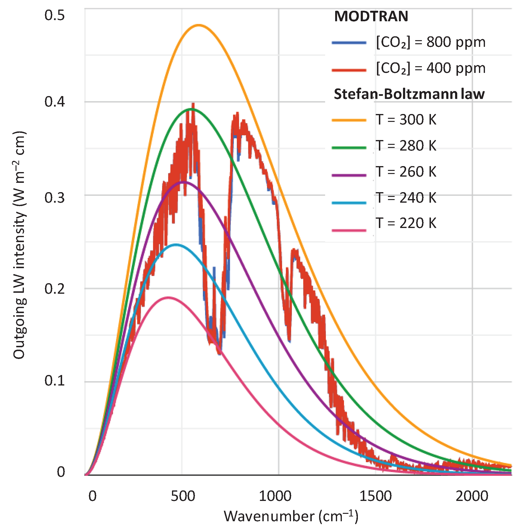
A typical graphical output of the MODTRAN application is seen in Figure 1. This is for the standard tropical atmospheric profile, also in comparison to the case that the standard [CO₂] of 400 ppm is replaced by that of 800 ppm (the difference is difficult to discern).
As the MODTRAN web application only models the longwave radiation, in a case where the shortwave (SW) radiation was needed in this study, this was estimated by another model, RRTM (standing for Earth's Energy Budget), again available as a web application by the University of Chicago [48]. This simulates both LW and SW radiation fluxes, both upward and downward.

3. Data

To compare MODTRAN results to observed radiation profiles in the atmosphere, we need radiosonde data. While radiosondes are routinely made in several hundreds of sites across the world, they typically measure temperature, humidity, pressure and wind. Radiation radiosonde measurements are rare, yet it is useful to make at least a single comparison to get a general idea. Here we use a couple of radiosondes from a day and a night flight on 23 September 2011, in cloud-free conditions, at the aerological station in Payerne, Switzerland (6.9440° E, 46.8130°, +491 m a.s.l.). In these, in-situ measurements of downward and upward radiation fluxes were taken through the troposphere and into the stratosphere, exceeding 32 km of altitude. They were presented by Philipona et al. [49] in graphical form in their Figure 2, which was digitized here to recover the measurements.
For the downwelling LW radiation flux, there have been numerous measurements at specific sites and for a period of more than a century [18]. These were the basis for the derivation of the empirical or semiempirical formulae for the calculation of the downwelling radiation flux, discussed in Section 2.2. Considering that these formulae reflect the data that was based upon, here we use the formulae, instead of the data, for comparisons with MODTRAN.
Information for the radiation fluxes at the top of the atmosphere (TOA), including the LW fluxes, are provided by satellite instruments. These are available only for the 21st century from the ongoing project Clouds and the Earth’s Radiant Energy System (CERES), a part of NASA’s Earth Observing System, designed to measure both solar-reflected and Earth-emitted radiation from the TOA (in CERES defined at the altitude of 20 km) to the surface.
The specific product used here is the CERES SSF1deg monthly averaged TOA LW radiative fluxes at a 1°-regional grid, constant-meteorology-temporally-interpolated [50,51,52]. The TOA fluxes are provided for clear-sky and all-sky conditions. Both these observational data are available online [53] and were retrieved here for their entire time span of complete years, i.e., from January 2001 to December 2022 from the Terra platform. The same CERES product provides information on clouds, which was also retrieved (monthly averaged for both day and night).
In addition, the CERES project provides LW fluxes for the surface, both downwelling and upgoing, through the product CERES_EBAF_Ed4.2, where EBAF stands for “Energy Balanced and Filled” [54,55]. However these are computed gridded values rather than observational data. They are publicly available [56] and were also retrieved here.
The CERES data are associated with considerable uncertainties. According to CERES [57], the combined regional all-sky LW flux uncertainty is 2.4 W/m² and the daily regional all-sky LW diurnal uncertainty is 8 W/m². According to CERES [58]; Table 6.1], the uncertainties in the 1°×1° regional monthly TOA fluxes are 4.6 W/m² for clear sky and 2.5 W/m² for all sky. In addition, as also noted in CERES [58], with the most recent CERES instrument calibration improvements, there still is a net imbalance of ~4.3 W/m², much larger than the expected observed ocean heating rate which CERES assumes to be ~0.71 W/m². It is noted though that, according to the calculations by Koutsoyiannis [22], the latter imbalance value, again inferred from ocean heating data, is even lower, 0.37 W/m². The EBAF dataset adjusts the observations to remove the above inconsistency. All this information suggests that the observational uncertainties are far too high to allow calculations of Earth’s imbalance and of temporal climatic changes, yet they are quite useful for the scope of this study.
Additional atmospheric variables used here, namely temperature and water vapour pressure, are taken from the ERA5 and NCEP/NCAR Reanalyses at monthly scale. ERA5 stands for the fifth-generation atmospheric reanalysis of the European Centre for Medium-Range Weather Forecasts (ECMWF; ECMWF ReAnalysis). Its data are publicly available for the period 1940 onwards at a spatial resolution of 0.5°. NCEP/NCAR stands for Reanalysis 1 by the National Centers for Environmental Prediction (NCEP) and the National Center for Atmospheric Research (NCAR). Its data are publicly available from 1948 to the present at a horizontal resolution of 1.88° (∼ 210 km). Both data sets can be retrieved from the Climexp platform [59] and from the Physical Sciences Laboratory platform of the US National Oceanic and Atmospheric Administration (NOAA) [60]. Finally [CO₂] data were retrieved for the most well-known station, Mauna Loa, again from the Climexp platform.
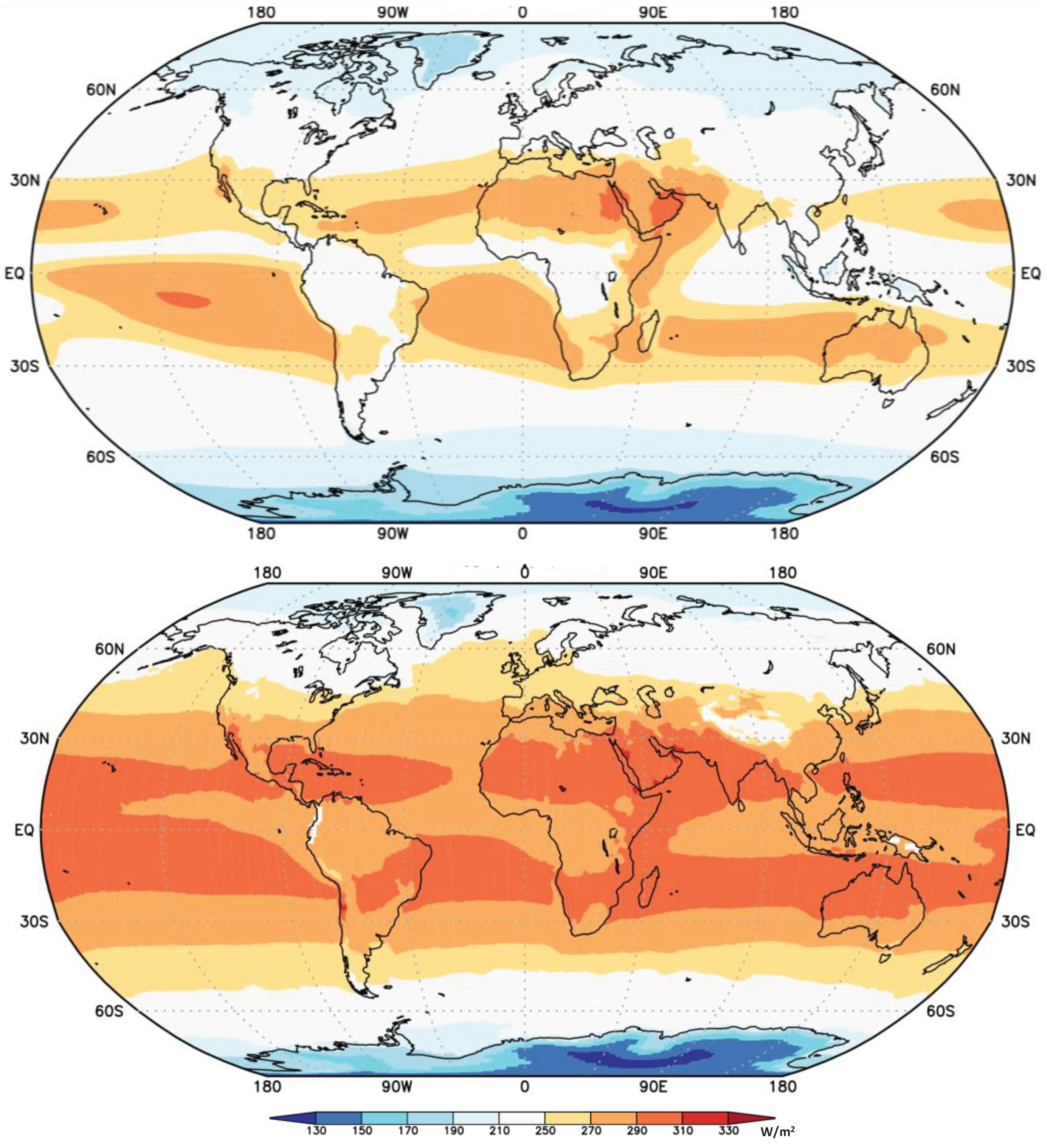
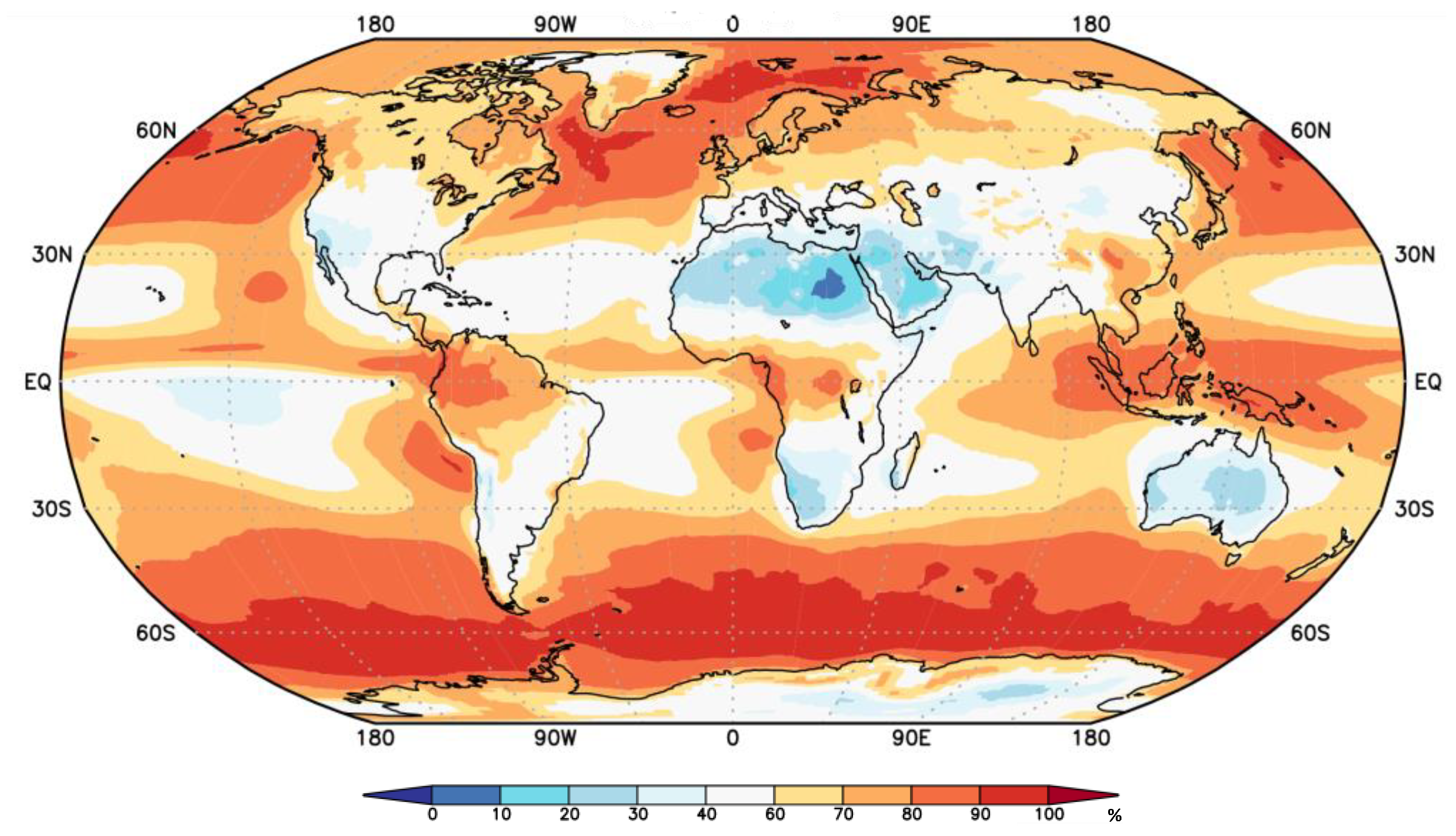
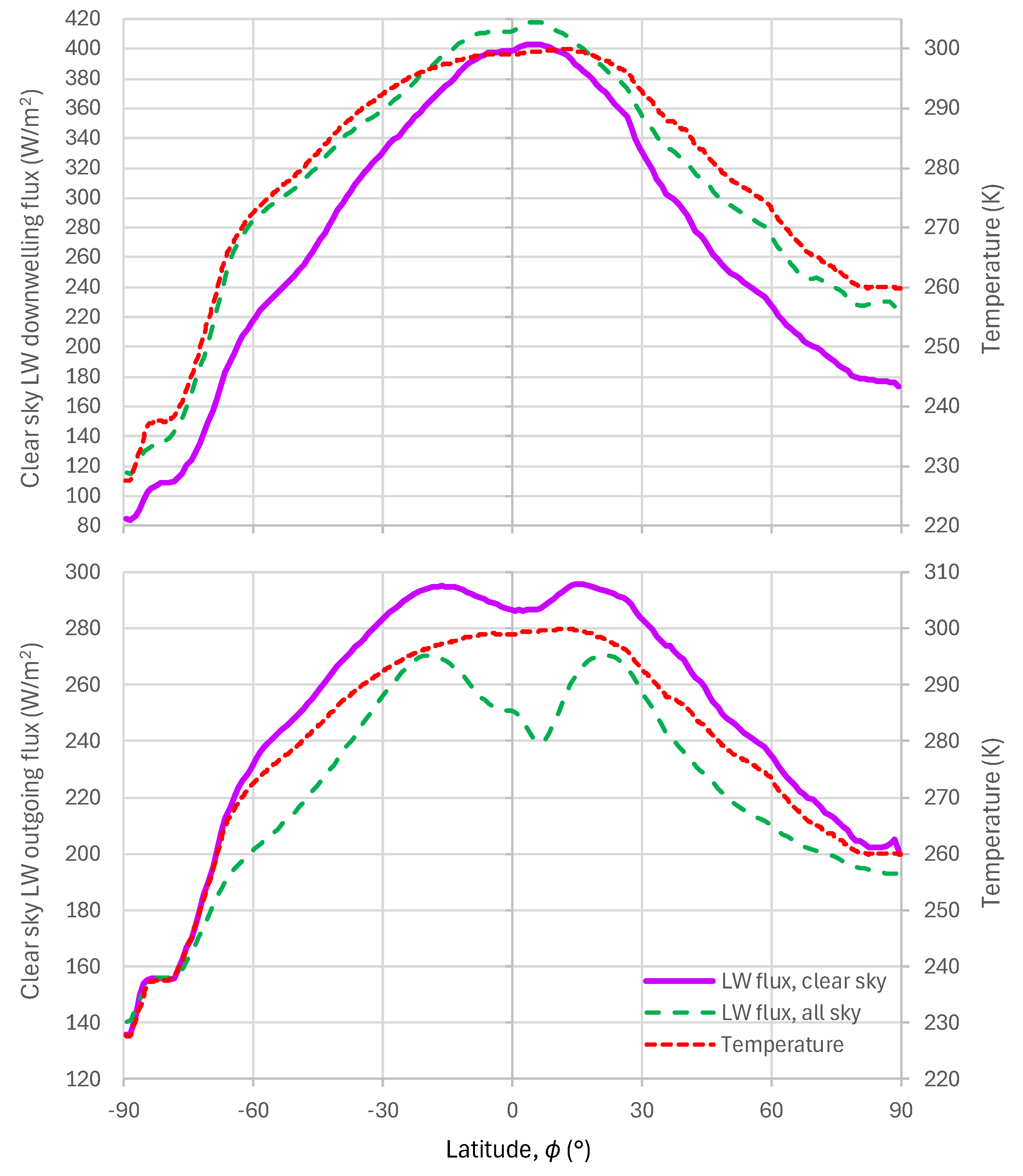
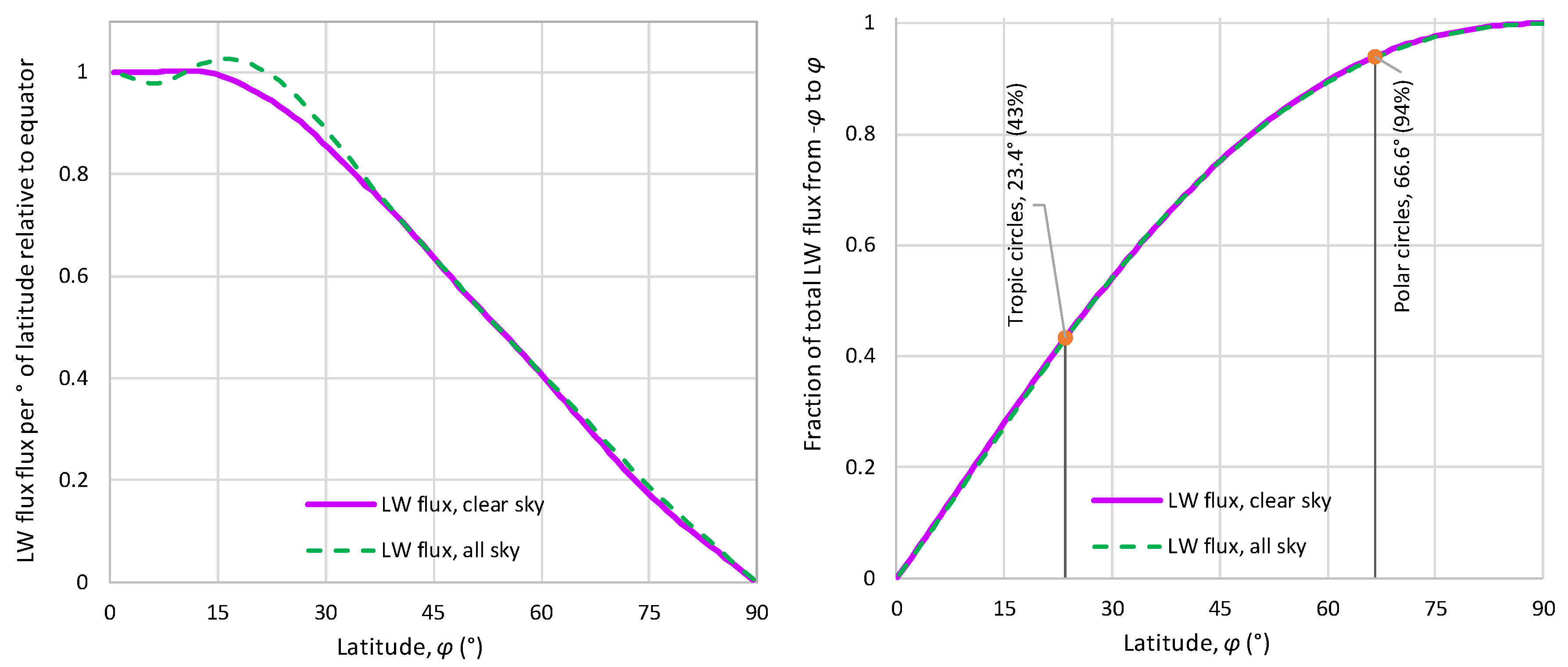
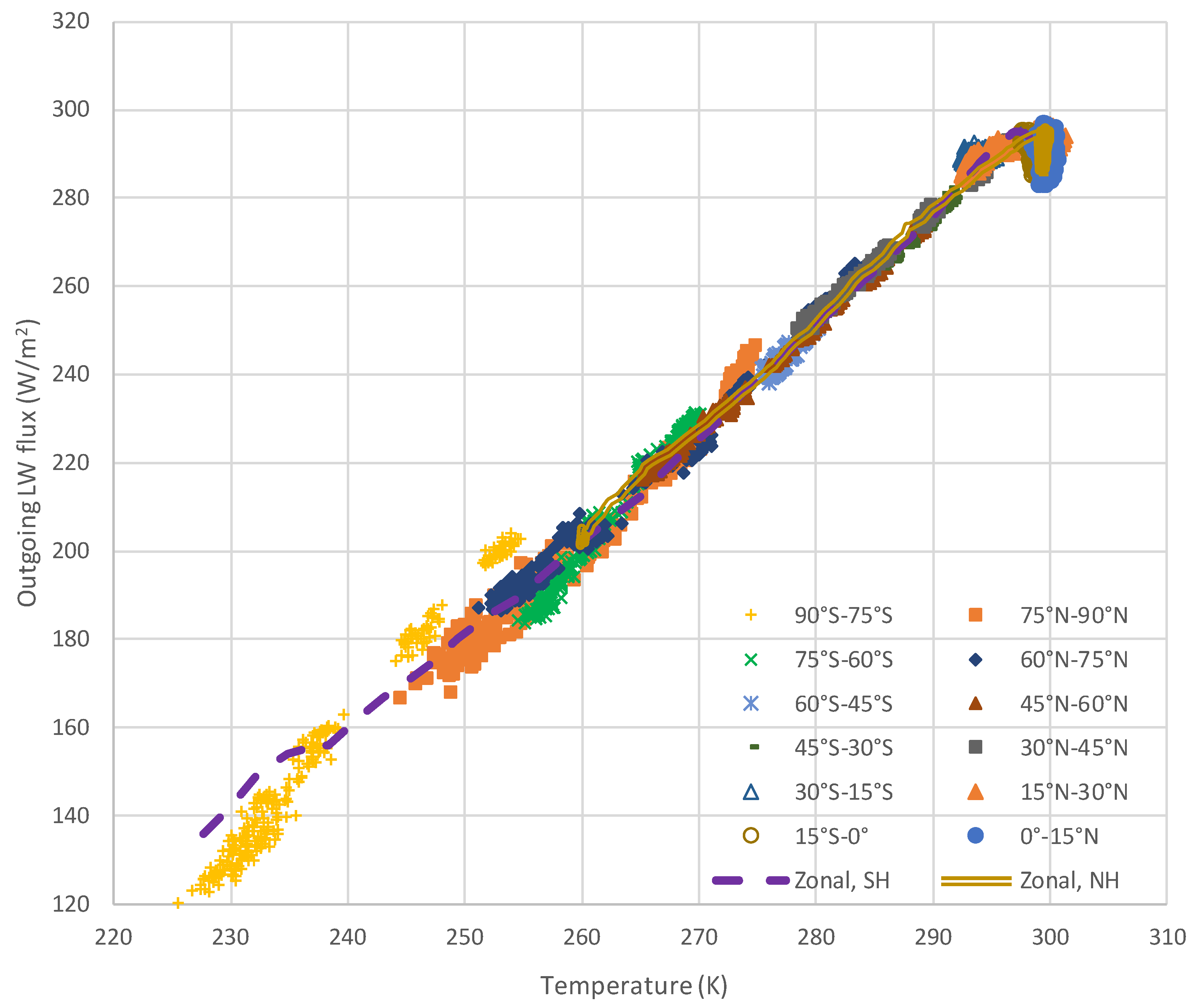
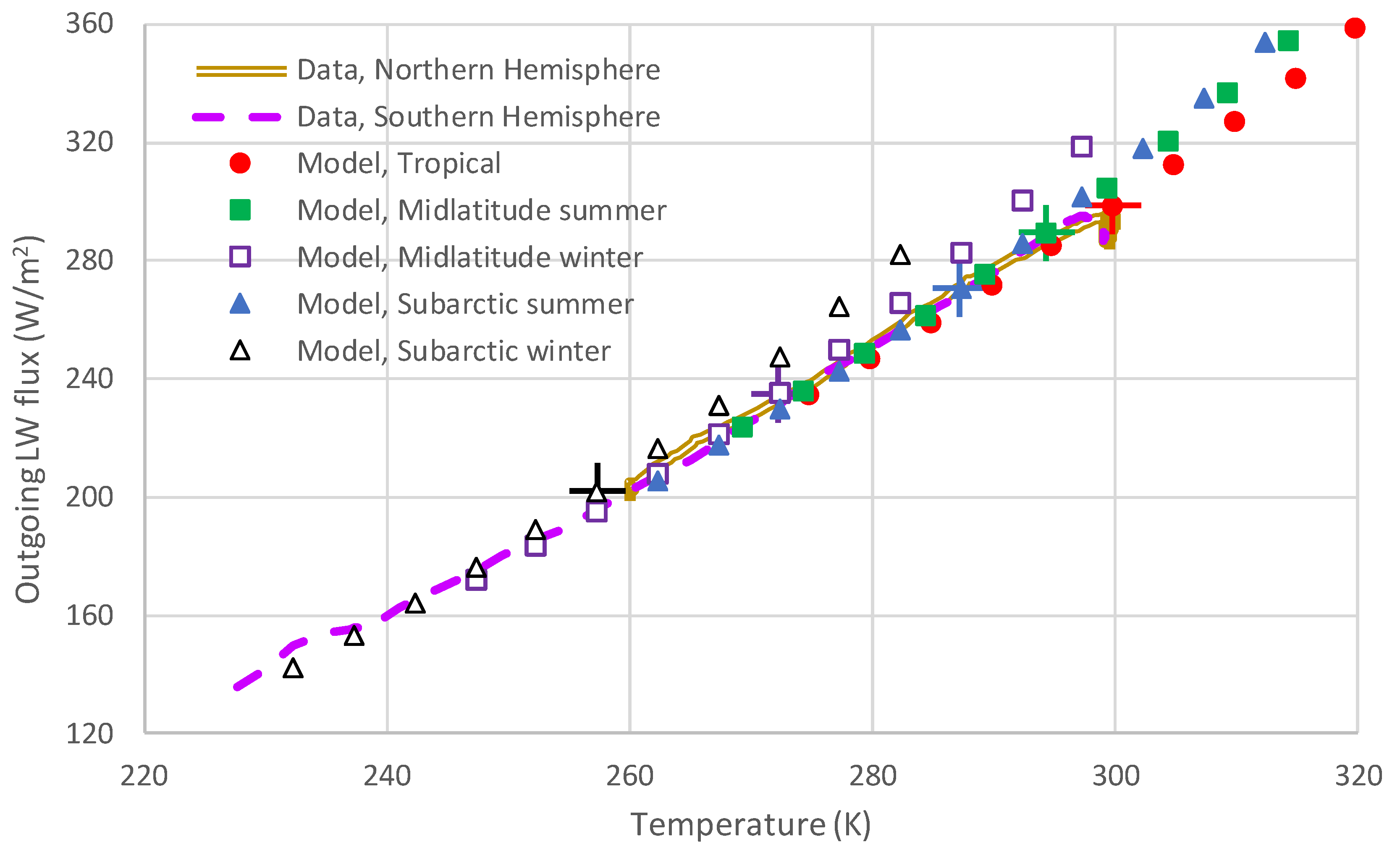
The gridded CERES SSF1deg TOA LW data are presented in Figure 2, averaged over the period of observations. The cloud information (cloud area fraction) of the same data product is shown in Figure 3. The zonal distribution of the LW radiation data are shown in Figure 4, along with that of temperature, and, as expected, the distributions of the two variables are similar. Figure 5, constructed from the data of Figure 4 shows that the torrid zone (between 23.4° S and 23.4° N) contributes 43% of Earth’s outgoing LW radiation flux, and together with the two temperate zones (between 23.4° and 66.6° S and N) radiates 94% of the total, leaving only 6% for the frigid zones (between 66.6° and 90° S and N). Figure 6 better depicts the relationship of outgoing LW radiation flux and surface temperature, for each month of the 22 years of data availability separately, but areally averaged over geographical zones of 15° latitude. This graph allows two important observations. First, the individual monthly values align very well with the average zonal distribution. Second, at the high end of temperature variation, around 300 K, there appears a stagnancy, or even regression of radiation with respect to temperature.

4. Macroscopic Relationships

4.1. Clear-Sky Relationships

Faithful to Dooge’s [61] spirit of “looking for hydrologic laws”, i.e., simple macroscopic laws for phenomena whose details are complex, this section tries to establish relationships between the downwelling and outgoing LW radiation fluxes with the variables that influence it, namely, temperature, water vapour pressure, carbon dioxide concentration and cloudiness. To this aim it primarily uses MODTRAN outputs and also cloudiness information.
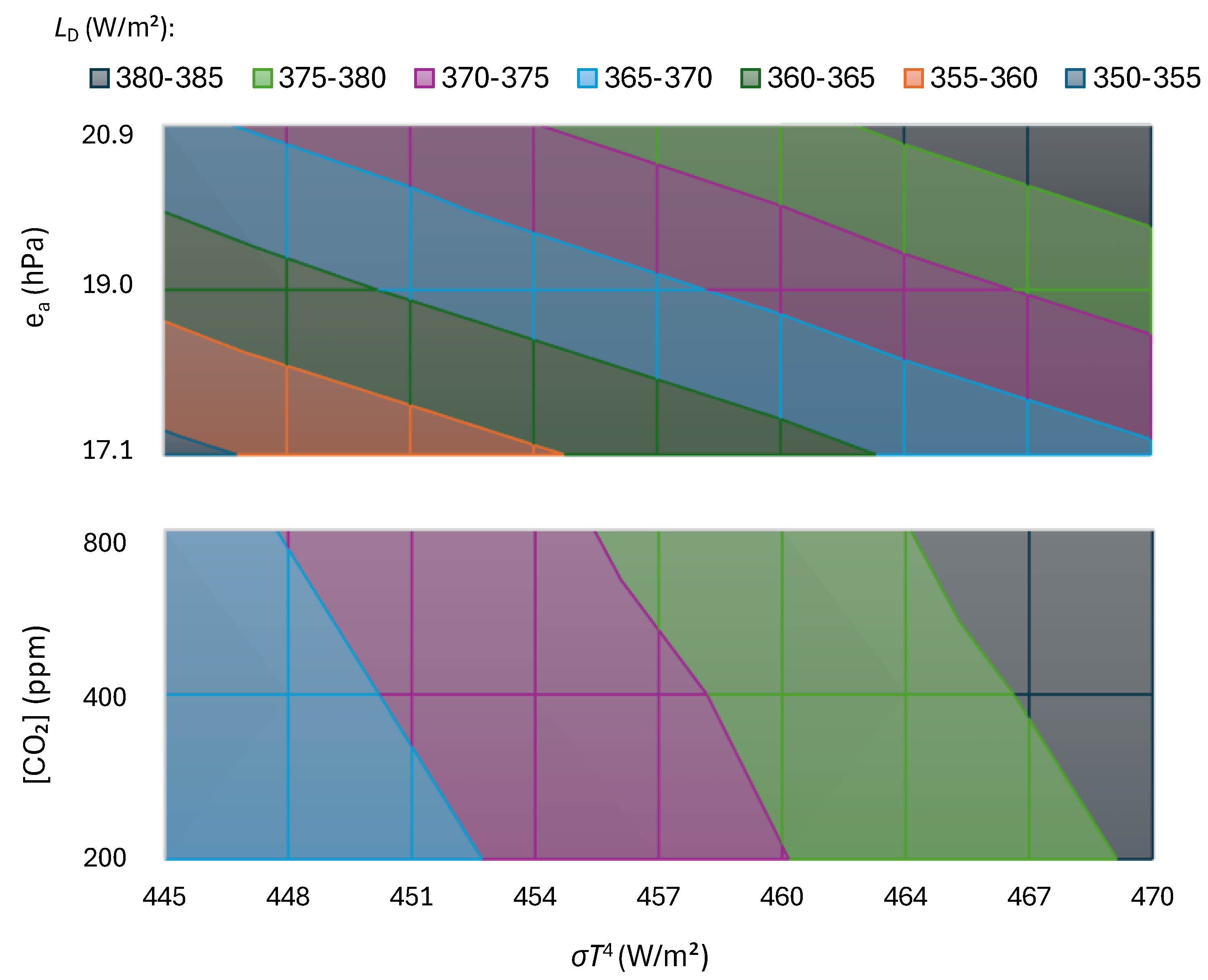
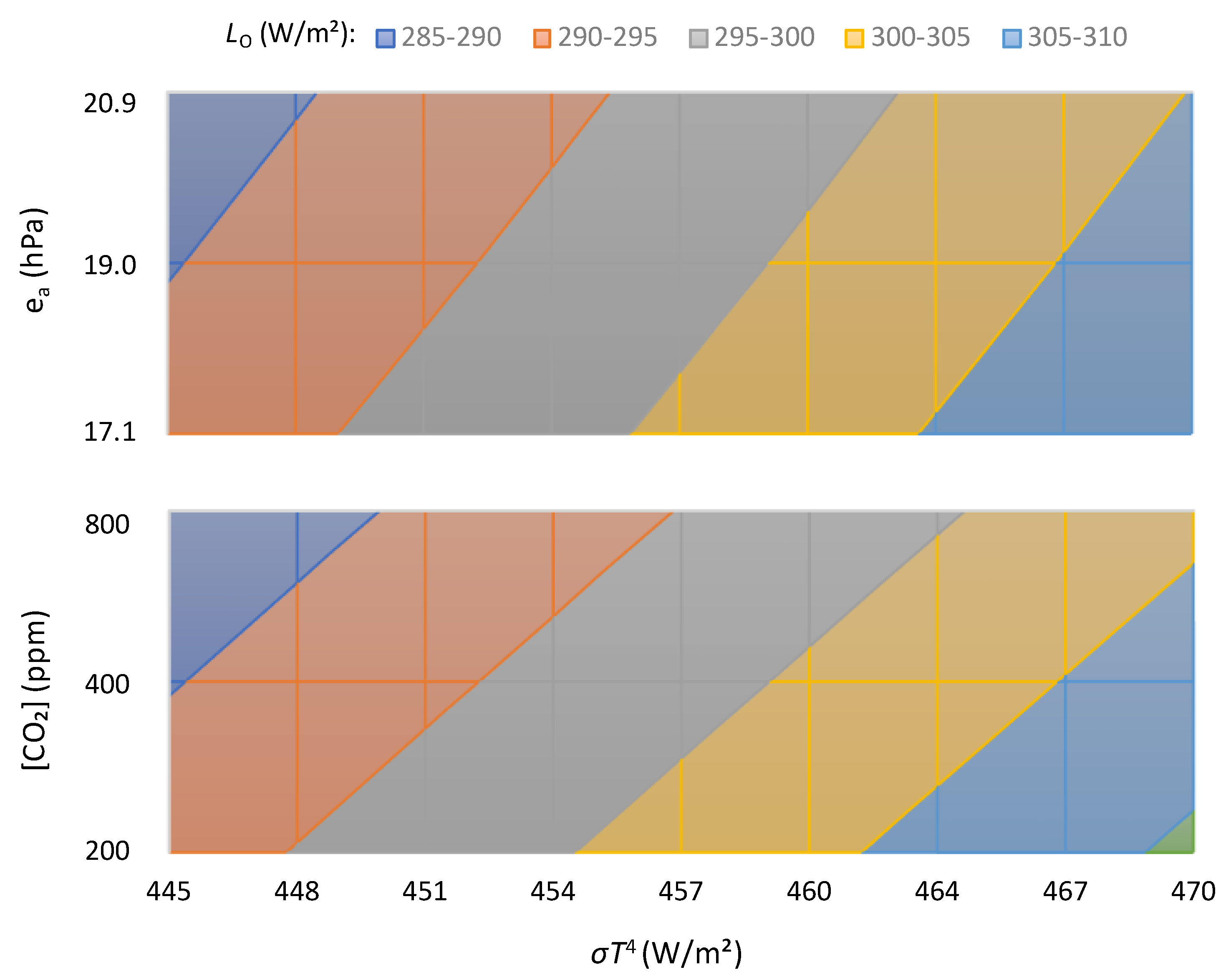
A series of systematic MODTRAN runs around the values of the standard tropical profile, i.e., [CO₂] = 400 ppm and for surface T = 299.7 K and e a = 19 hPa, with ranges of 200 – 800 ppm for [CO₂], ± 2 K for T and ± 10% for e a , gave the results shown in contour graphs in Figure 7 for the downwelling LW flux and in Figure 8 for the outgoing flux. Both figures suggest that the relationships among the involved variables are simple and that macroscopic representations are possible. Figure 7 shows a linear effect of e a and a logarithmic one of [CO₂] on the variation the downwelling LW flux. In addition, it shows that a ± 10% change in e a is larger than a doubling or halving of [CO₂]. Similar are the results of Figure 8, but with smaller differences of the effects of the two factors.
Based on these preliminary results, several mathematical expressions were formulated and fitted. The following equation was found to be the best for both the downwelling and outgoing flux, L D and L O , respectively:
L D , O = L * 1 + T T * η Τ ± e a e a * η e 1 ± a C O ln C O 2 C O 2 0 ( 1 ± a C C )
with C O 2 0 = 400 ppm. This includes two groups of parameters to be optimized, namely (a) dimensional, L * , T * , and e a * with units [L], [T], and [ e a ], respectively, and (b) dimensionless η Τ , η e , a C O and a C . Excepting the last one, referring to the cloud area fraction, C, and discussed in Section 4.2, all others were optimized based on clear-sky MODTRAN results, and their values are contained in Table 1.
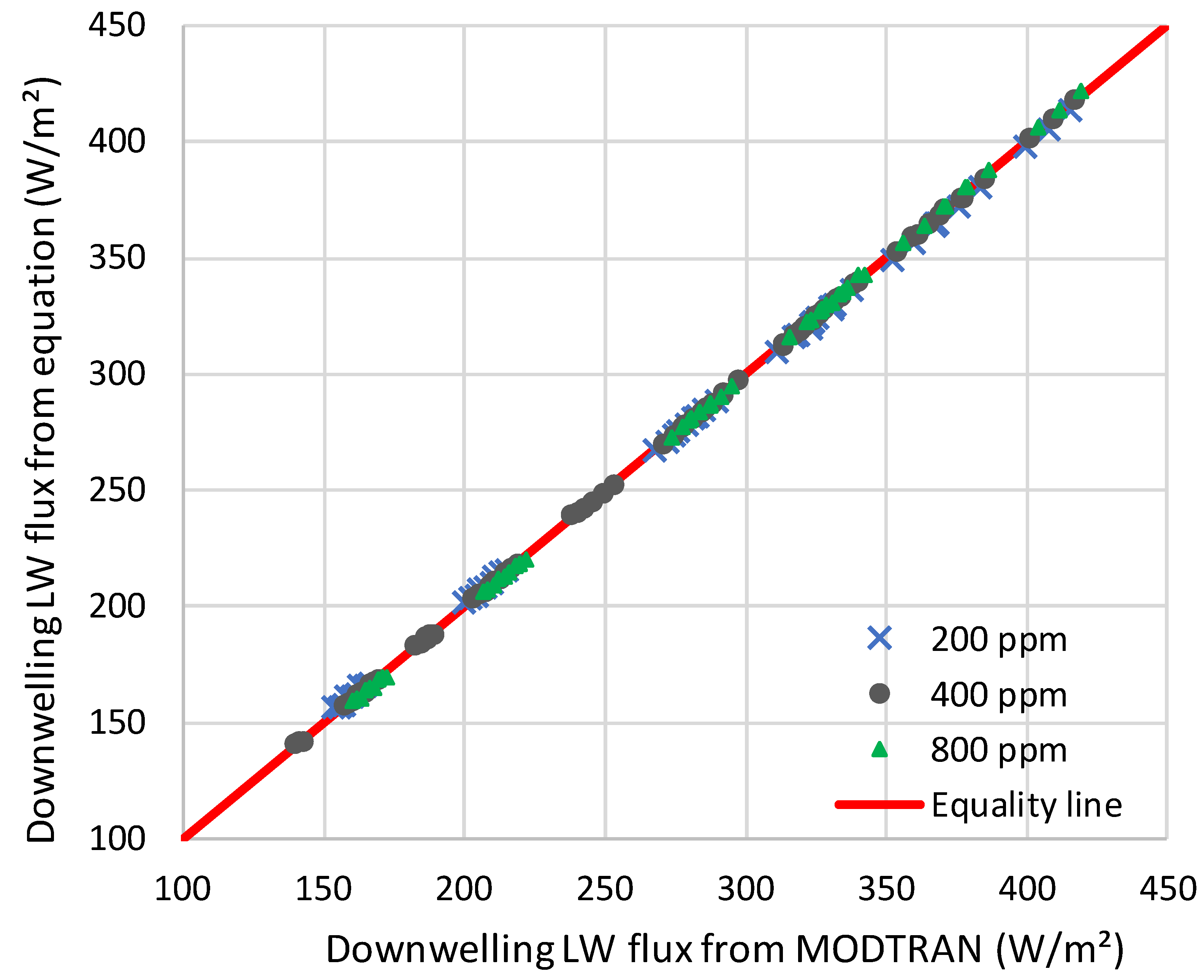
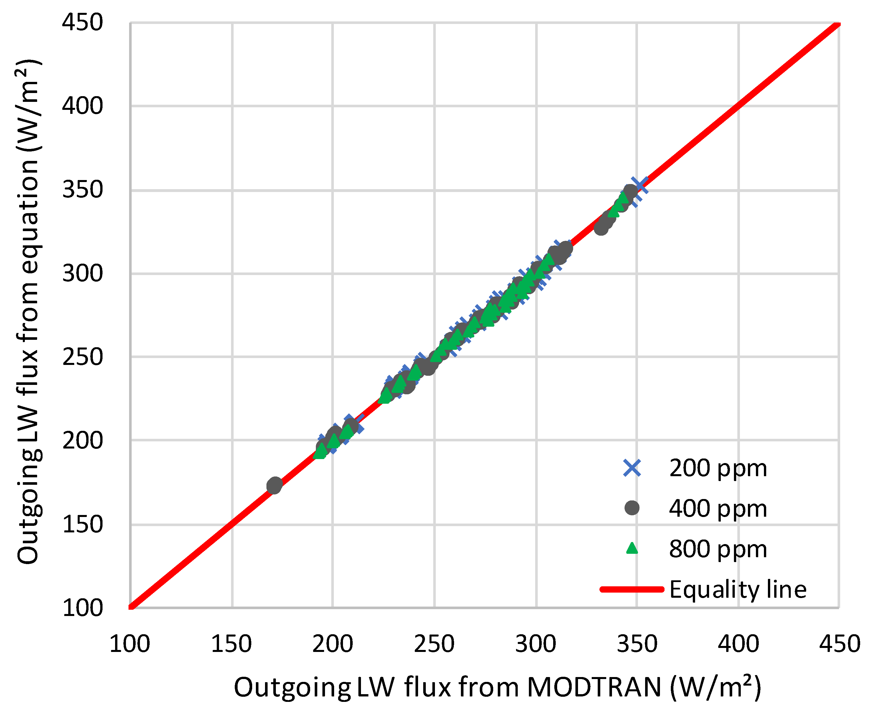
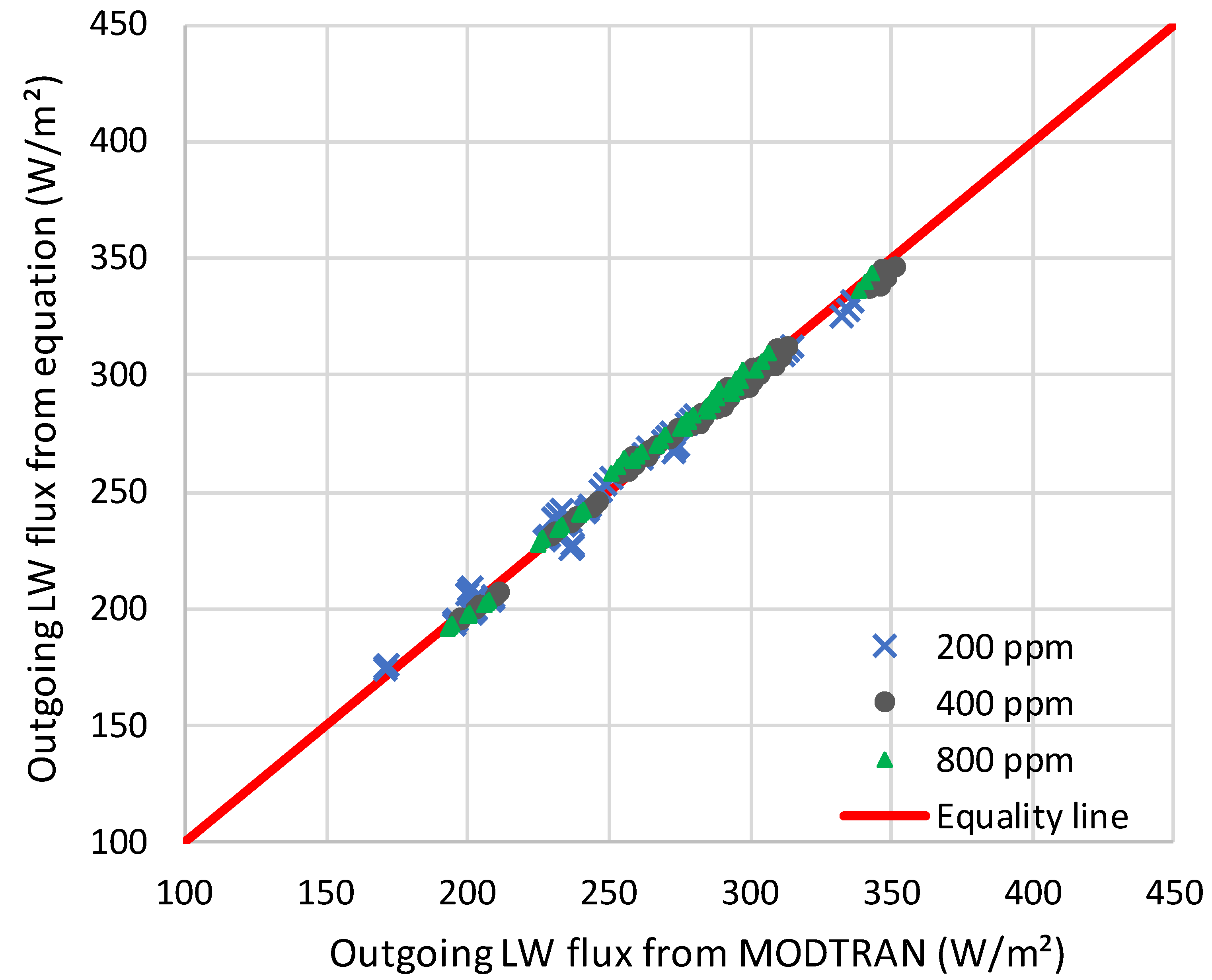
As seen in Table 2, the performance measures of the fitting are very good and hence the equation is a good macroscopic representation of the MODTRAN results. The good performance is also seen graphically in Figure 9 for downwelling flux and Figure 10 for outgoing flux.
For completeness, an additional equation was formulated, which directly relates the outgoing to the downwelling radiation. It is very simple:
L O = L s L a 2 + 40   W / m 2
where to calculate the surface radiation flux L s the emissivity taken ε s = 0.97 . The performance of Equation (22) is also good, albeit inferior to that of Equation (21), as seen in Table 2 and Figure 11. This equation shows that the outgoing and downwelling flux are closely (and negatively) related to each other.

4.2. Effect of Clouds

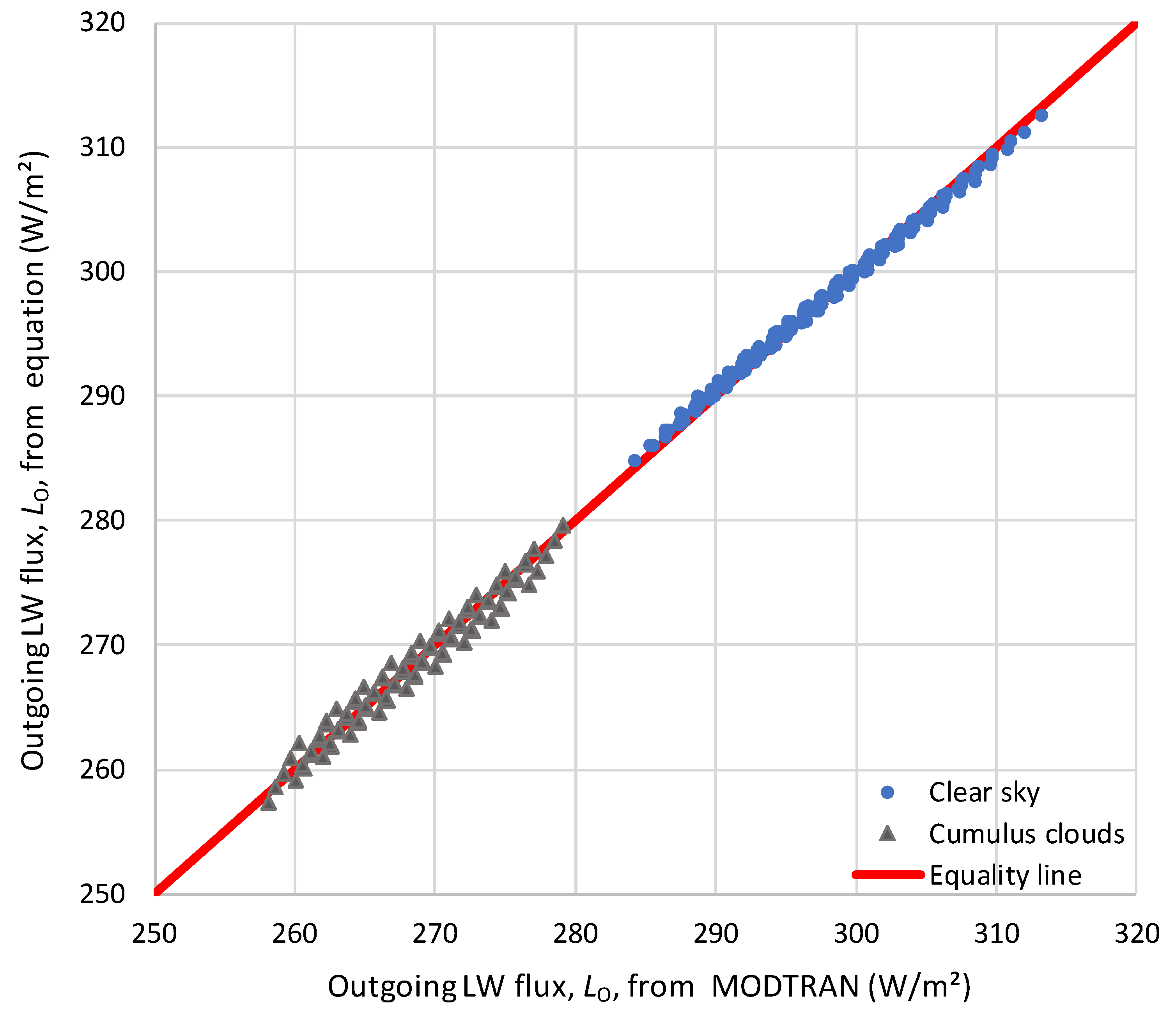
MODTRAN offers the possibility to model different types of clouds, in addition to clear-sky conditions. Figure 12 shows an example for cumulus clouds and the tropical profile. In particular, it shows that Equation (21) with 1 a C C = 0.904 (standing for the ratio of outgoing radiation under cloudy sky to that of clear sky) also represents well the case of cumulus clouds without changing the parameters. Similar performance appears for other types of clouds, but with different ratios, which are shown in Table 3 for the different types of clouds and locality profiles.
However, it is important to test whether these ratios agree with observed ones. From the CERES data sets, the global average LW radiation flux for the entire observation period, 2001 – 2022, is L O C S = 268.2 W/m² for clear sky and L O A S = 239.5 W/m² for all sky, and give a ratio of 0.892. On the other hand, the global average cloud area fraction, again calculated from the CERES data, is C = 0.671. We assume that the following approximation holds:
L O A S L O C S = 1 a O C
from which we find a O = (1 – 0.892) / 0.671 = 0.161. For C = 1 , we would have L O A S / L O C S = 0.839. Comparing the latter value to those in Table 3, we understand that the MODTRAN model severely underestimates the effect of clouds, as even the least value of the ratio in the Table (0.887 for altostratus clouds and the subarctic summer profile) is too high in view of an average of 0.839. Therefore, to model the effect of clouds we use the CERES data rather than the MODTRAN results, based on the simple relationships:
L O C = L O 1 a C C ,             L D C = L D ( 1 + a C C )
where L O and L O C denote the outgoing LW radiation flux for clear sky and cloudiness C, respectively (and likewise for the downwelling, L D and L D C ) and a C parameter, which may take different values for different situations. These relationships are already incorporated in Equation (21).
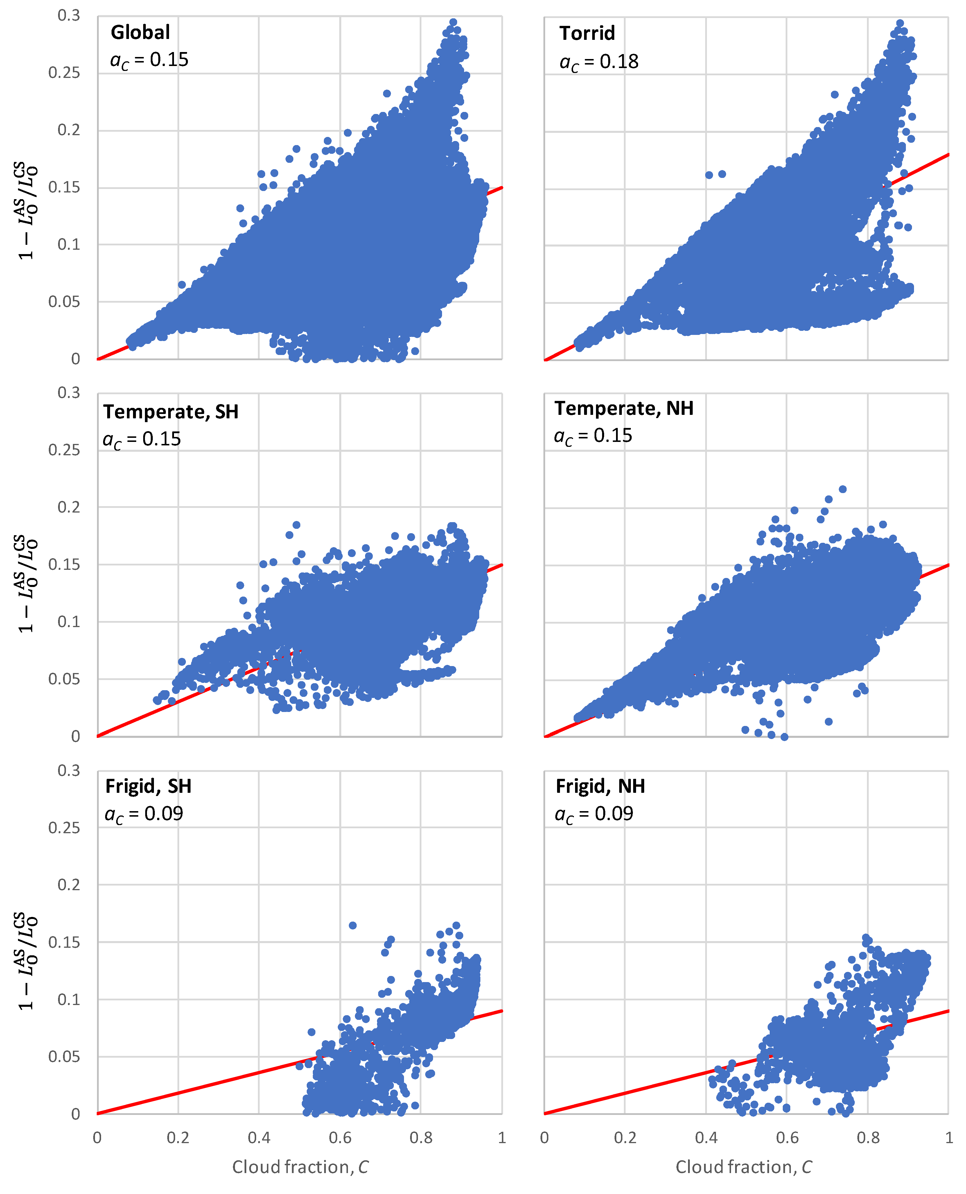
To determine the parameter a C for the outgoing LW radiation we investigate the CERES data (clear and all sky, and cloud fraction, globally and in the five different geographical zones, as shown in Figure 13. The resulting a C values are also shown in the Figure and vary from 0.18 in the torrid zone to 0.09 in the frigid zones. Notable is the large spread of the observations, with a variation range of 0 to about twice the estimated mean slope (i.e., 1 L O A S / L O C S from 0 to 0.30).
The data used in this study do not allow direct estimation of a C for downwelling flux and thus we use values from literature. Dingman [62], p. 189] suggested a value of 0.4, Jacobs [63], p. 108] estimated a value of 0.33 and Lhomme et al. [64] a value of 0.34. (This could be also taken as 0.37 as the formula in their equation (13) can be written as is L D C / L D = 1.03 + 0.34   C , w h i c h f o r C = 1 y i e l d s L D C / L D = 1 + 0.37 .) Of these values, here we use a C = 0.34 as this value was based on the most extensive data set and is most recent. Other researchers give different formulae [65](p.142),40,42], but here we preferred the simplest linear formulation.

5. Test Results

5.1. Radiation Flux Profiles

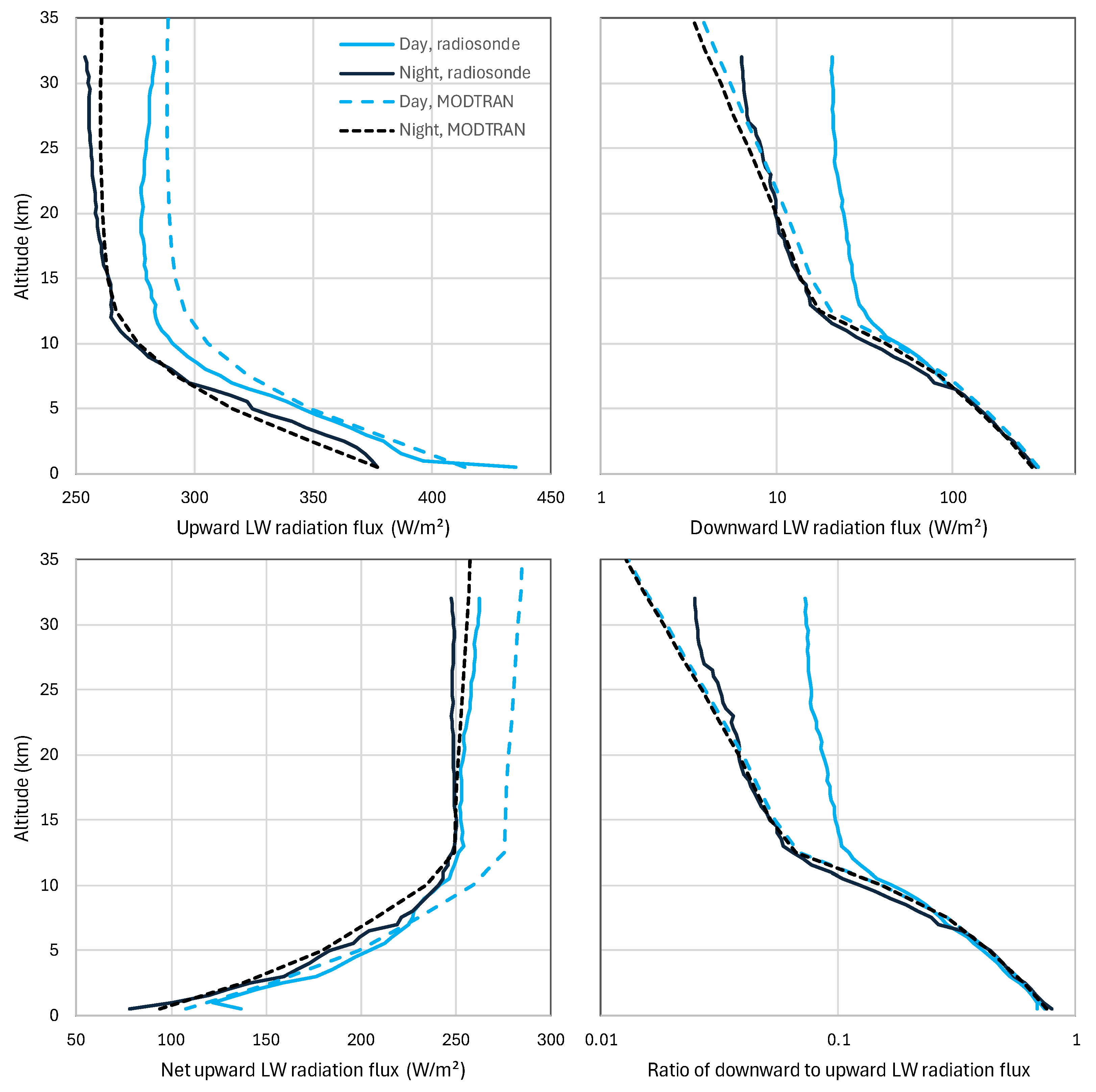
As already mentioned (Section 3), the most appropriate way to test the validity of a model that determines the LW radiation, such as MODTRAN, would be to compare its results to observed radiation profiles. As described in Section 3, here we make a single comparison to get a general idea, using the two radiosondes launched on 23 September 2011 at Payerne, Switzerland, and reported in the study by Philipona et al. [49], whose LW radiation profiles were digitized here. As reported in the study, the surface-emitted LW upward radiation was about 445 W/m² during the day, with a remarkably strong decrease during the first 1 km, and 380 W/m² during the night. A surface temperature of 11 °C (284.2 K) is reported in the study for 23 September 2011, without clarifying whether this corresponds to the day or night radiosonde. Using MODTRAN with the standard midlatitude summer profile, we find that at the altitude of +0.5 km, the values of 445 W/m² and 380 W/m² are achieved for a temperature offset of +5.5 K (297.5 K at +0.5 km) and –6.2 K (285.8 K at +0.5 km, close to the reported 284.2 K), respectively. However, the former temperature offset gives too high temperature at higher altitudes, inconsistent with the observed strong decrease across the first 1 km. Therefore for the comparison of the day profile with MODTRAN we did not use any temperature offset, while for the night case we assumed an offset of –6.8 K (285.1 K, midway of the values 284.2 K and 285.8 K).
Figure 14 depicts the radiosonde profiles, compared with the MODTRAN results obtained with the above assumptions. For the night radiosonde, there is a good agreement, yet the differences between observations and MODTRAN results are ±25% for the downward flux and ±4% for the upward flux. For the day radiosonde, the differences are substantial, particularly above 7 km. Philipona et al. [49] attribute these differences to the thermal longwave radiation from the Sun—a plausible interpretation. Excepting the latter factor, we may deem that MODTRAN represents the relevant processes satisfactorily.

5.2. Downwelling Radiation

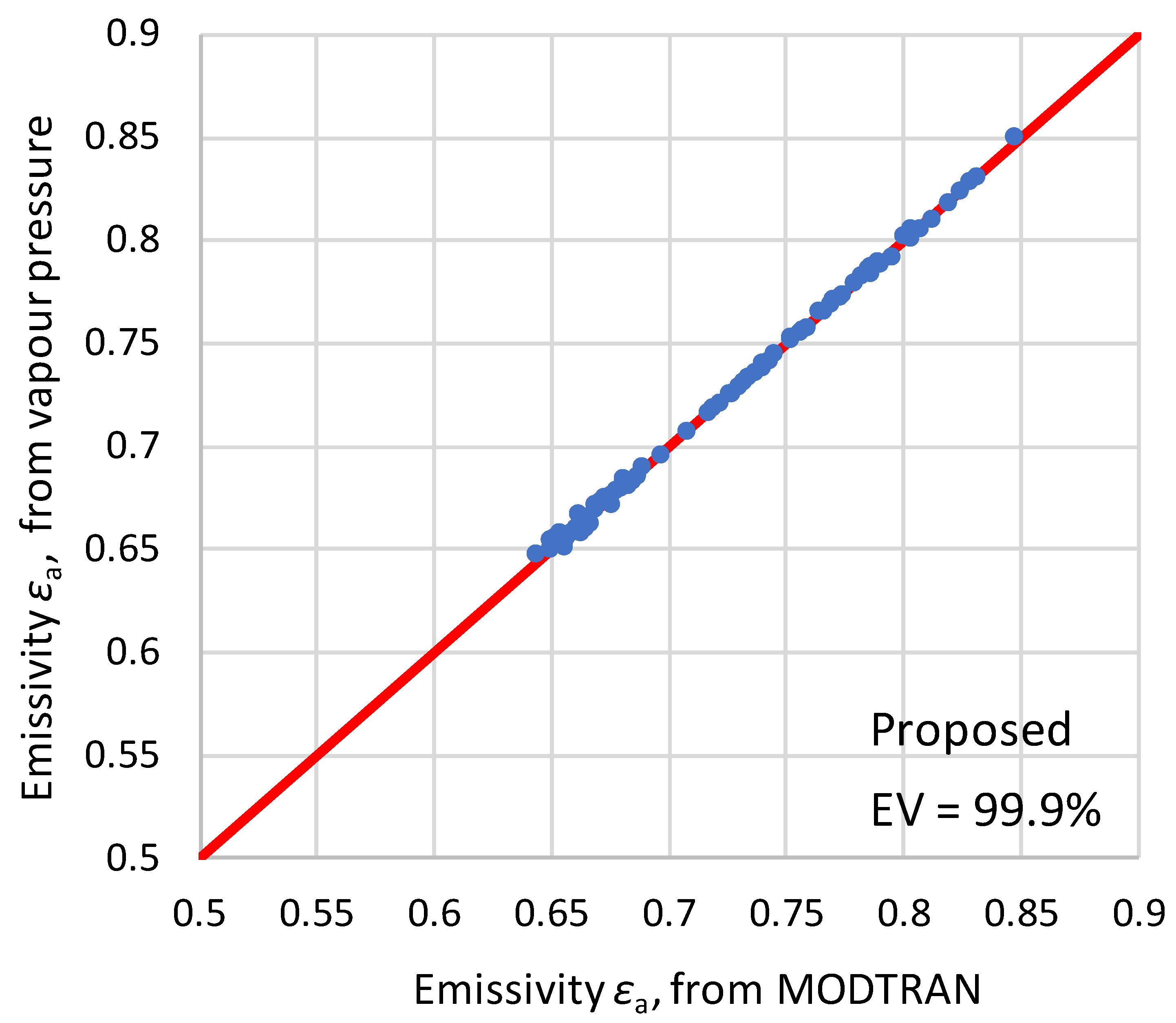
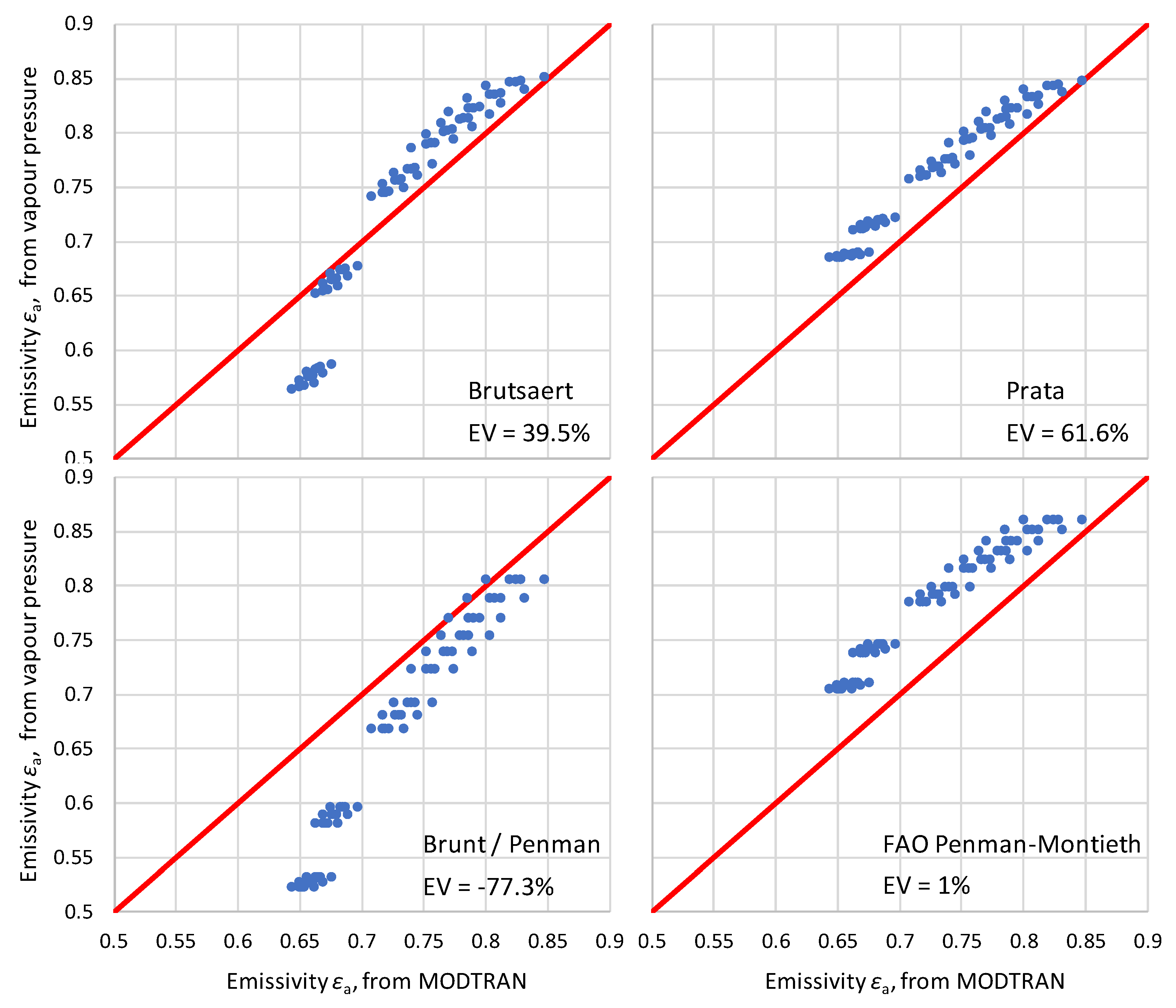
As already mentioned, we use the empirical or semi-empirical formulae of downwelling radiation to test the MODTRAN results. These formulae are expressed in terms of emissivity ε a = L a / σ T a 4 (Section 2.2). Figure 15 shows that the emissivity calculated by the macroscopic relationship of Equation (21) perfectly agrees with that directly calculated by MODTRAN (explained variance, EV = 99.9%). As seen in Figure 16, the agreement is not so good if we compare MODTRAN’s emissivity with those of the formulae in Section 2.2. The best agreement (EV = 61.6%) is seen for Prata’s Equation (15) followed by Brutsaert’s Equation (13) (EV = 39.5%) and the FAO Penman-Montieth’s Equation (20) (EV = 1%). The Brunt / Penman Equation (18) gives an EV < 0, meaning that a single value equal to the mean performs better than the relationship in representing the compared data.
Note that if the group of points corresponding to subarctic winter with temperatures lower than 270 K is excluded, Brutsaert’s equation has the best performance of all, with an explained variance of 75%. Overall, if we assume that the empirical or semi-empirical formulae are closer to reality than MODTRAN because they are based on data and if we exclude the subarctic winter data (and the Brunt / Penman equation) we conclude that MODTRAN underestimates the downwelling radiation flux.
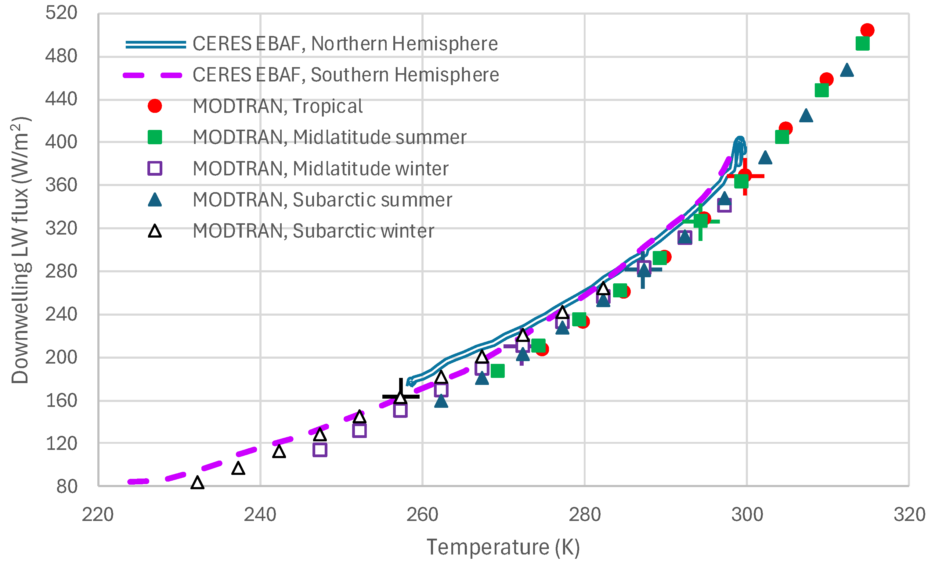
Another comparison is made in Figure 17 for the downwelling LW radiation flux vs. temperature, as calculated by MODTRAN and the CERES EBAF zonal distribution shown in Figure 4. For the former all five locality profiles are used with default settings as well as with temperature offsets from the default values of up to ±25 K. We recall that CERES EBAF data are not actually measurements but computed results. Yet the graph suggests a tendency of MODTRAN to underestimate the downwelling radiation, a finding similar to that in the comparison with the emissivity formulae.

5.3. Outgoing Radiation

For the outgoing radiation, a comparison similar to that in Figure 17 is made. It is presented in Figure 18 and is now stronger and more meaningful, as the CERES outgoing LW flux is observed, rather than computed. The graph shows that at the default temperature values of each of the MODTRAN profiles there is almost perfect agreement between CERES data and MODRTAN results, and this is also extended for negative temperature offsets in MODRTAN. However for positive temperature offsets, MODRTAN overestimates the flux.
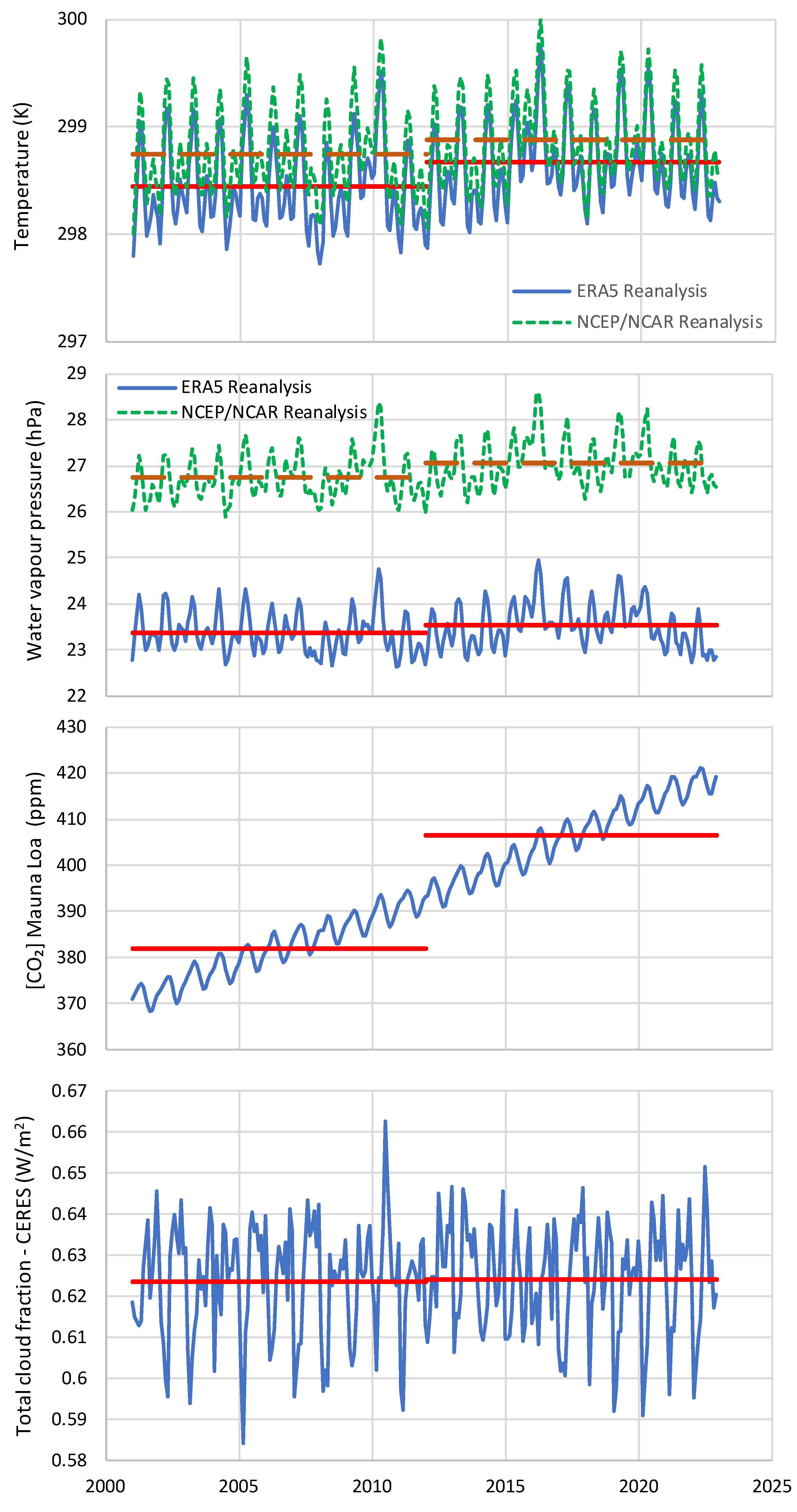
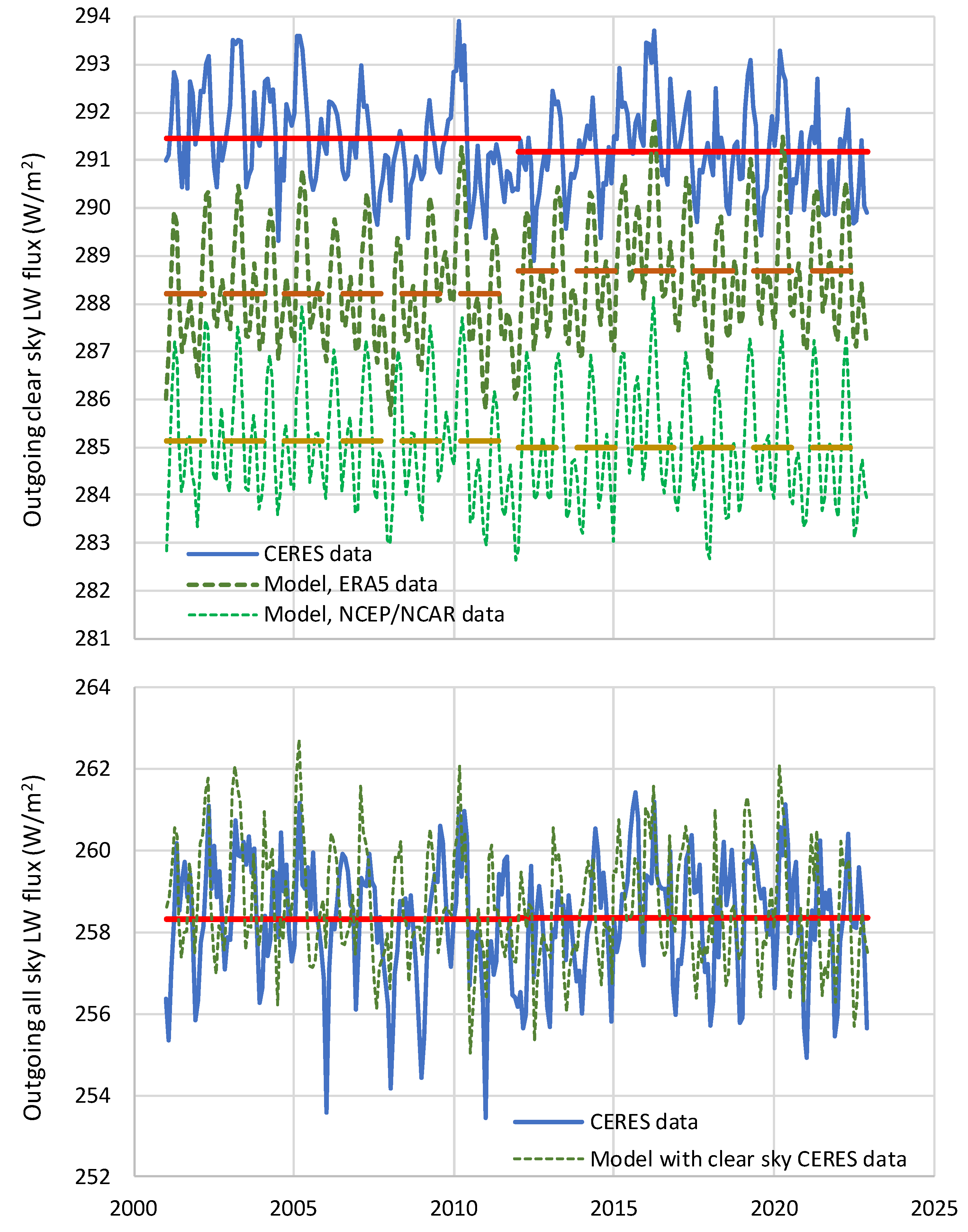
As another test, we use time series of meteorological variables and [CO₂] for the 22 years of CERES data availability averaged over the torrid zone, which are shown in Figure 19. For temperature and water vapour pressure, both ERA5 and NCEP/NCAR reanalyses data are used, which, as shown in the graphs have differences from each other, particularly in the latter variable. Based on these time series and Equation (21), the model results, which correspond to MODTRAN, are calculated and plotted in Figure 20. In the upper panel of the Figure, substantial differences are seen in the mean levels of the clear-sky LW outgoing radiation, both between the time series of the two reanalyses and the latter with the CERES data. These can be attributed mostly to uncertainty in Reanalyses results and their representation of reality, as indicated in the differences between the two. If we exclude the effect of the mean level differences, the cross-correlation coefficients with the CERES data are reasonable, i.e. 0.67 for ERA5 and 0.69 NCEP/NCAR.
In the lower panel of Figure 20, we use the CERES clear-sky time series, as shown in the upper panel, and multiply it by the quantity ( 1 a C C ) of Equation (21), with a C = 0.18 (the value of the torrid zone) and cloudiness C as in the time series of the lowest panel of Figure 19. The attained results compare well with the all-sky CERES time series in terms of mean level, even though the cross-correlation between the two plotted time series (–0.15) does not suggest correspondence of the individual monthly values.
Both in Figure 19 and Figure 20, the average values of the time series are shown for two 11-year subperiods, 2001 – 2011 and 2012 – 2022. It is seen that there were increases in the second period in all variables (very large in CO2 and very slight in all-sky outgoing radiation) except in the clear-sky radiation, where a slight decrease (–0.08 W/m2) is seen. It is interesting to investigate if the latter decrease is explained by MODTRAN. The results of the related calculations are shown in Table 4. Using any of its default profiles, MODTRAN results in increase of outgoing clear-sky LW radiation (from +0.38 to +0.60 W/m2), opposite to what is seen in the CERES data.
The above results from CERES data, which are for the torrid zone only, are similar to those for global averages, presented by Koutsoyiannis and Vournas [18; Appendix B]. The latter study also examined SW radiation data and found a decrease of total outgoing radiation, which is consistent with the increased atmospheric temperature. This decrease of outgoing radiation can hardly be attributed to increased [CO₂] but it can be related to water vapour and cloud profiles. The effect of CO₂ is trumped by the effect of clouds, which is consistent with the major role of water on climate and the minor one of CO₂.

5.4. Final Assessment

The above tests illustrate the high uncertainties not only in the CERES LW radiation data, but also in the other atmospheric variables, and the relationships among them and the LW radiation, as represented in MODTRAN. The uncertainties do not allow accurate representation of quantities calculated as differences between different variables or between the same variables in different periods, such as in attributing changes. On the other hand, the macroscopic behaviour of MODTRAN seems consistent with what is observed for clear sky, and therefore MODTRAN is suitable for the scope of this paper, which is the investigation of the relative importance of carbon dioxide and water in the greenhouse effect, as detailed in the next section. As regards clouds, MODTRAN seems to underestimate their effect, but by using the cumulus or altostratus cloud conditions, we get results close to reality for average all-sky conditions.

6. Comparison of H₂O and CO₂

6.1. Imaginary-World Conditions

Investigating imaginary-world conditions seems pointless, yet we include it for the reasons explained in the Introduction—the fact that several popular narratives are based on imaginary-world conditions. The imaginary-world conditions we examine are the most extreme ones, starting from the case that [CO₂] is totally absent in the atmosphere and ending to the case where the atmosphere is composed of merely CO₂. Extreme ranges are also examined for other greenhouse gases, including water vapour.
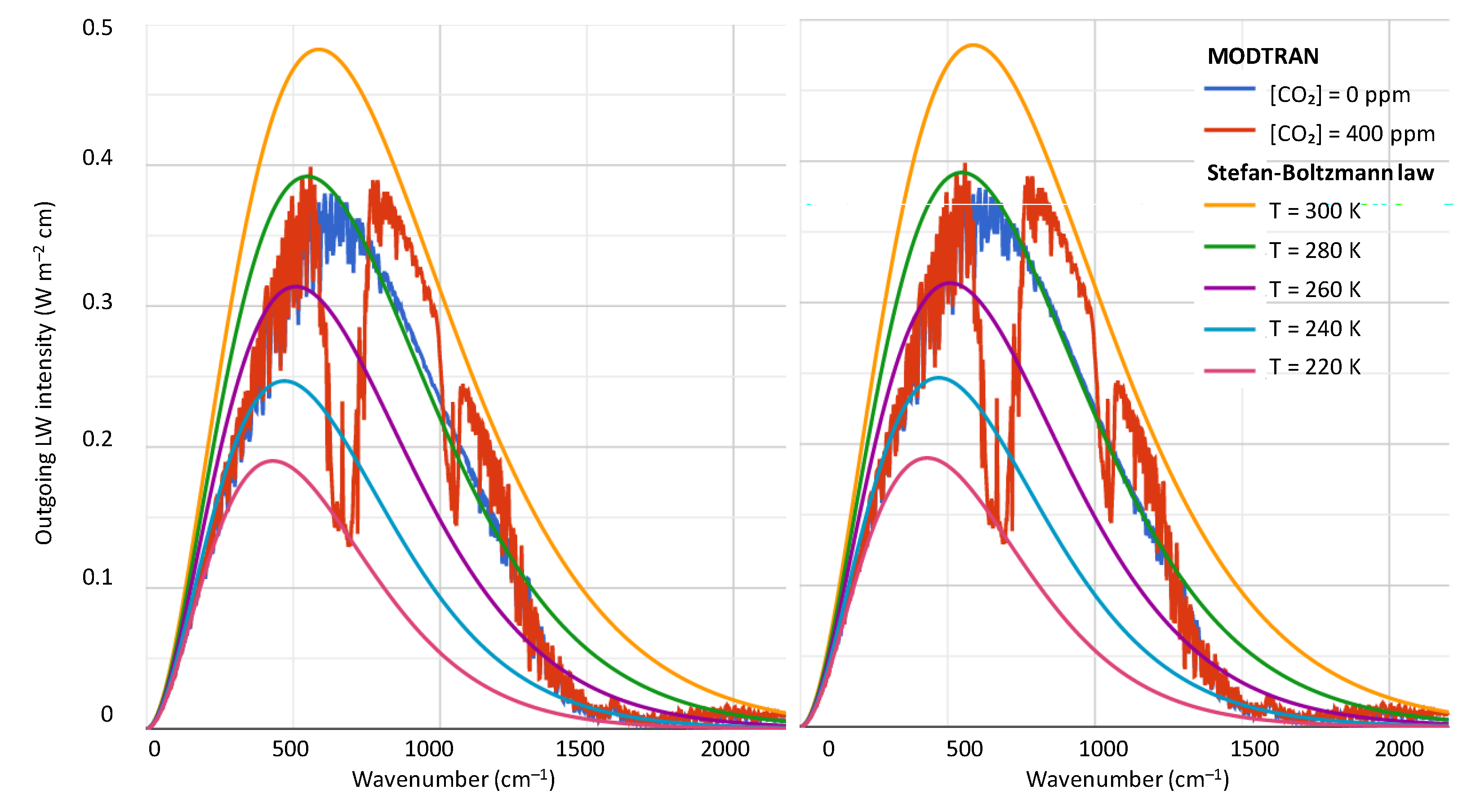
Figure 21 compares detailed MODTRAN outputs for the default case of the tropical profile, with [CO₂] = 400 ppm (and T = 299.7 K, L O = 298.49 W/m², water vapour scale = 1; red curves), compared to two cases in which CO₂ is totally absent (blue curves). In the left panel the water vapour is kept at the same level as in the default case. In order for the outgoing radiation to retain its default value ( L O = 298.49 W/m²), the temperature must be lowered by 15 K (T = 284.7 K). Notably, by also zeroing water vapour, to match the total outgoing LW flux of the red curve ( L O = 298.49 W/m²), the temperature should be lowered by 28.5 K (T = 271.2 K, case not shown in the figure but easily imagined in the middle between the smooth curves of 260 and 280 K). The right panel shows that the temperature can remain at its default value (T = 299.7 K) if water vapour scale is increased to 1.3, accompanied by cumulus clouds. Note that the 30% increase of the water vapour scale does not violate thermodynamic laws, as the vapour pressure remains below the thermodynamic limit. Therefore, assertions that the terrestrial greenhouse effect would collapse without CO₂ (see Introduction) are false.
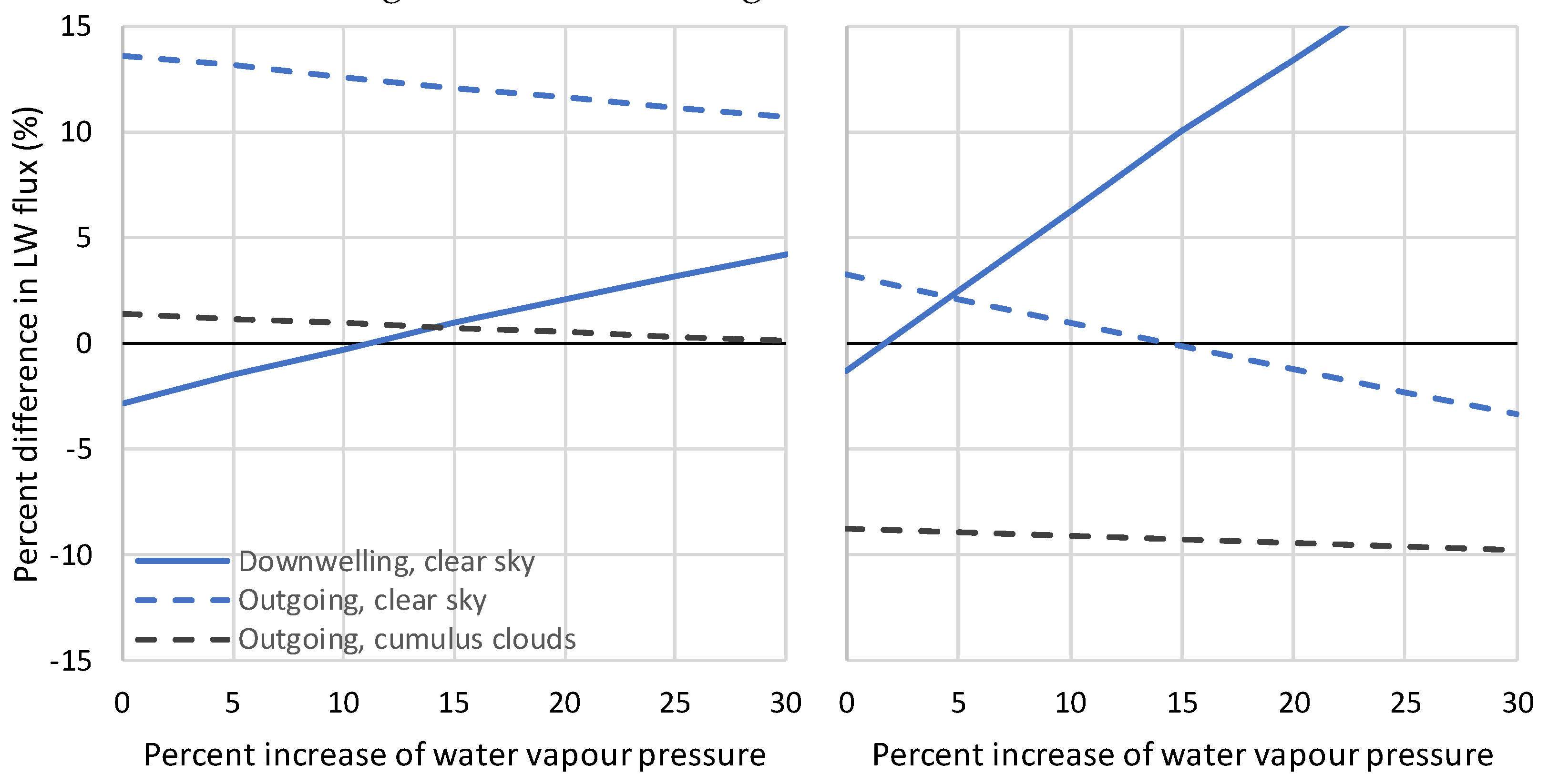
The fact that the greenhouse effect would not collapse without CO₂ is also shown in Figure 22 (left panel), which gives a more macroscopic picture for both downwelling and outgoing LW flux, under constant temperature equal to that of the standard tropical atmospheric profile (T = 299.7 K) and zero concentrations of all greenhouse gases except water vapour. It is seen than even without any change in the water vapour profile, the difference of LW radiation flux from the value at the default settings of [CO₂] = 400 ppm is only –3%. With a 10% increase of the water vapour and zero [CO₂], the downwelling radiation matches that for [CO₂] = 400 ppm.
Additional imaginary-world conditions are shown in Table 5. It can be seen there that by removing the entire quantity of atmospheric CO₂ we can achieve the same level of greenhouse effect, as produced by [CO₂] = 400 ppm and zero water vapour, with merely 0.15% of the current H₂O level in terms of upward and downward LW heat flux at the surface, or 4% in terms of the outgoing LW heat flux at 100 km altitude. On the contrary, it is impossible to approach the values of greenhouse effect achieved by merely H₂O in the atmosphere at the current level, by removing it and replacing it with CO₂. Even in an atmosphere entirely composed by CO₂ (i.e. 1 000 000 ppm or 2500 times the current CO₂ concentration) we cannot approach the greenhouse values achieved by merely the current level of atmospheric H₂O. On the other hand, we can easily achieve the greenhouse effect level of an atmosphere entirely composed by CO₂ with an atmosphere free of CO₂ and with only 20% of the current atmospheric H₂O for the downwelling radiation.
For completeness, we note that MODTRAN does not modify the temperature profile in case that water vapour is removed. It assumes a temperature gradient of 6.5 K/km, as in the standard atmosphere, or lower. However, without water vapour the temperature gradient would be the dry adiabatic one, i.e. 9.8 K/km (see Figure 25 discussed in Section 7), which signifies another effect of water vapour on the atmospheric processes. And of course, without water vapour, clouds would not exist and the surface cooling effect would be larger.

6.2. Realistic Conditions

Putting aside the imaginary-world cases of an atmosphere without CO₂ or one merely composed of CO₂, we may assume a realistic lowest value of [CO₂] of the order of 200 ppm. Redrawing the left panel of Figure 22 under this minimal value, instead of zero, we get what appears in the right panel. It is obvious that, in comparison to the [CO₂] level of 400 ppm the differences are small and can be easily counterbalanced by slight changes in water vapour pressure.
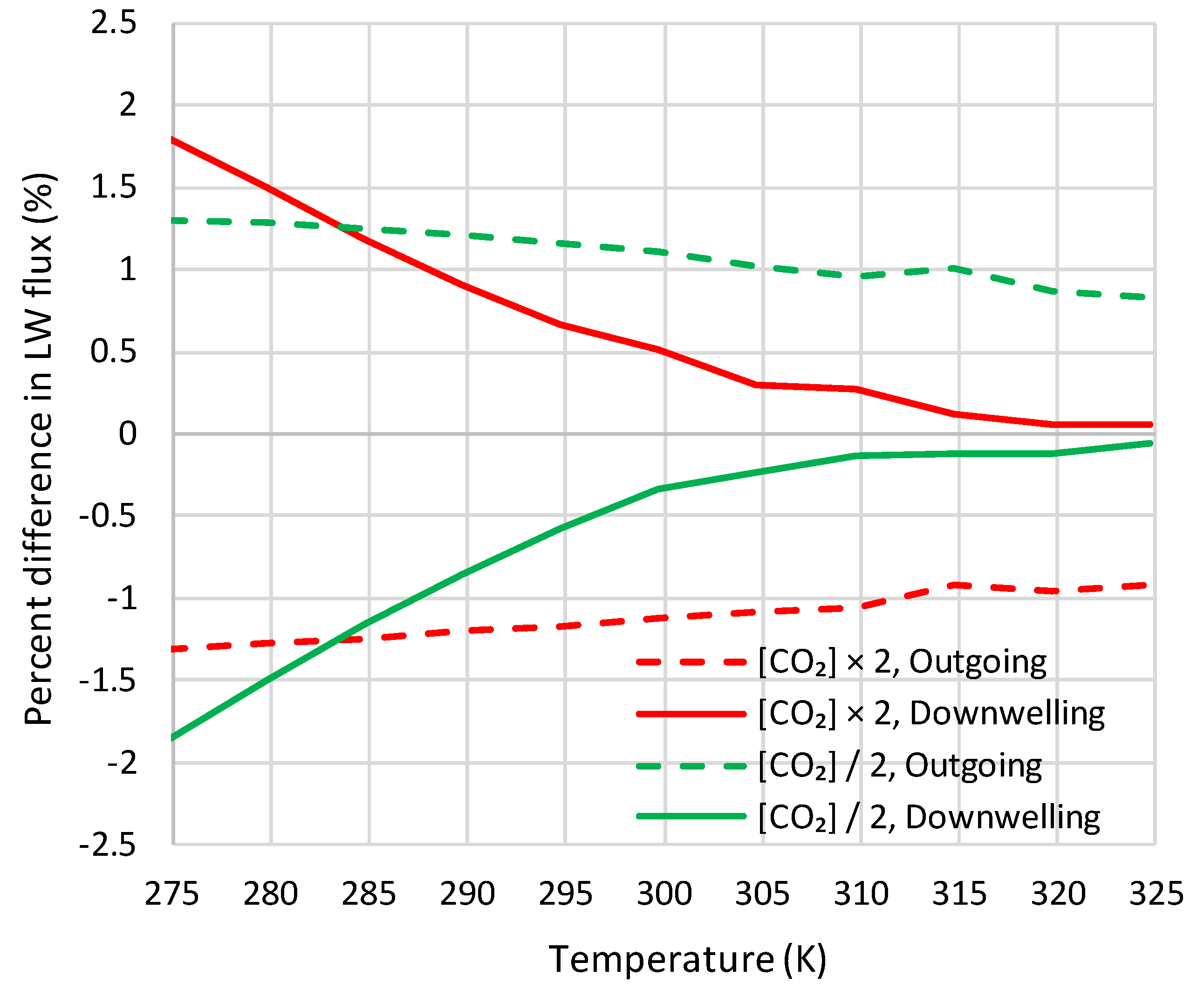
Another view of the same is provided by Figure 23, where the difference from the [CO₂] level of 400 ppm for two cases, doubling or halving this level, are presented. The differences are of the order of 1% and do not reach 2%.
For a more systematic investigation, we may determine the relative importance of each of the factors influencing the LW radiation flux, say factor F, by considering the relative change δ L / L produced by a relative change δ F / F in the factor F and taking the ratio:
δ L L / δ F F = δ L δ F F L L F F L = L F ' F L = : L F #
where L F   = L / F  and L F #   = ln L / ln F is the log-log partial derivative of L with respect to F (defined in [28], p. 97).
Equation (21) allows analytical determination of the log-log derivatives and hence the relative importance of each of the factors F T , e a , C O 2 , C . This is made in Table 6. MODTRAN also includes other greenhouse drivers with minor importance, i.e. CH4, tropospheric ozone, stratospheric ozone, and freon, which were not modelled in the above analyses. To calculate their bulk contribution, we increased each of the default values in MODTRAN by 5% ( δ A O / A O = 0.05 , where AO stands for “all other”), calculated δ L / L by MODTRAN for the tropical and subarctic summer profile (for comparisons) and applied Equation (25) to calculate L A O # , which resulted in values also included in Table 6; the relatively high value in the outgoing flux is primarily due to the influence of the stratospheric ozone.
It can be readily found using the values in Table 6, that the relative importance of water vapour over [CO₂] is 0.207/0.015 = 13.8 times for the downwelling flux, and ( 0.136 ) / ( 0.015 ) = 9.1 times for the outgoing flux. The relative importance of clouds over [CO₂] is 0.186/0.015 = 12.4 times for the downwelling flux, and (–0.112)/(–0.015) = 7.5 times for the outgoing flux. In other words, each of the related factors, water vapour and clouds, is an order of magnitude more important than [CO₂] in terms of the greenhouse effect.
Considering all above factors, the equation of total differential (with standard form d L = L / T d T + L / e a d e a + L / C O 2 d C O 2 + L / C d C + L / A O d A O ) can readily be written as
d L L = L T T L d T T + L e a e a L d e a e a + L C O 2 C O 2 L d C O 2 C O 2 + L C C L d C T + L A O A O L d A O A O
or,
d ln L = L T # d ln T + L e a # d ln e a + L C O 2 # d ln C O 2 + L C # d ln C
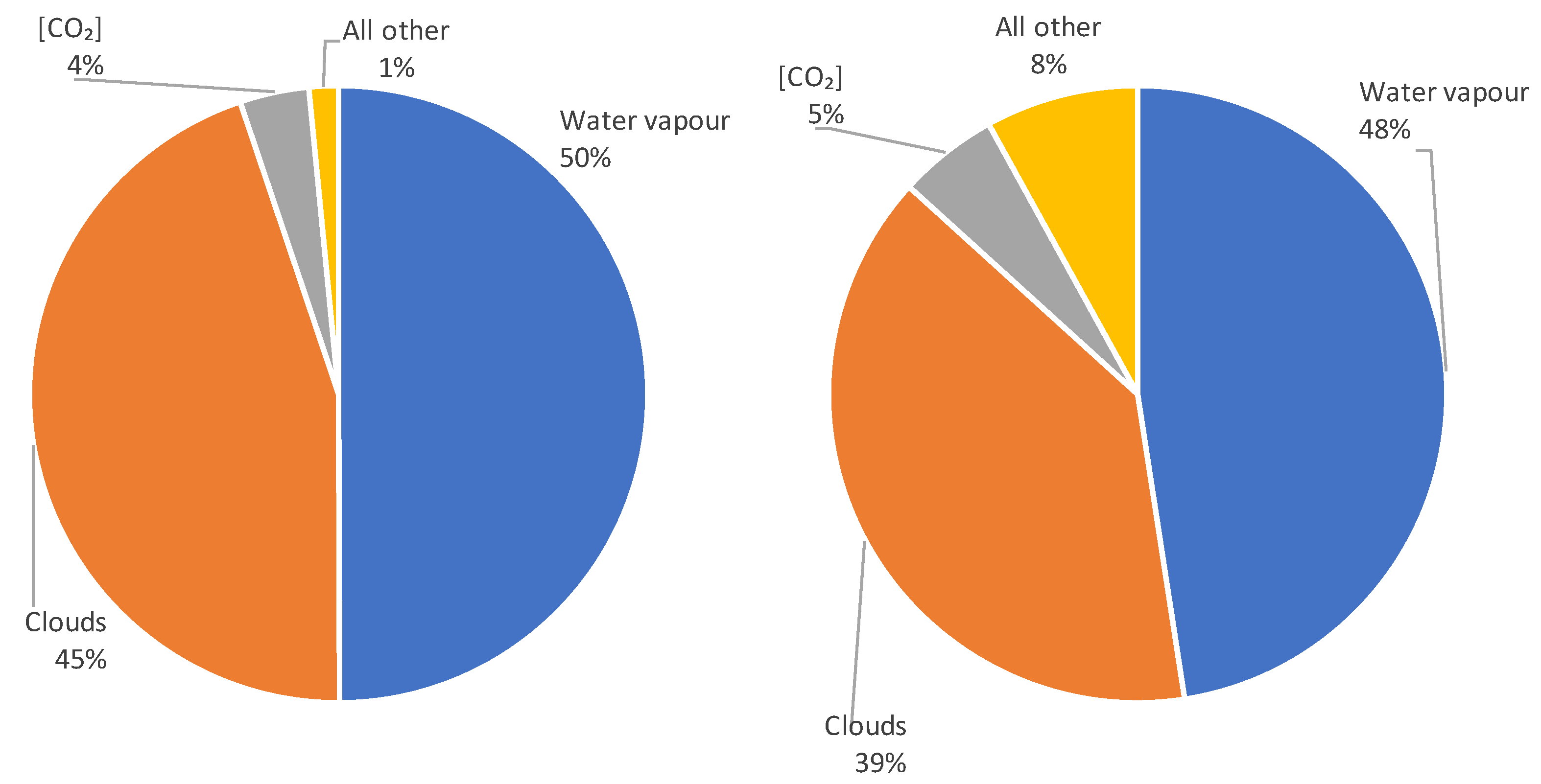
The first term in the righthand side, L T # , is by far the most important factor determining the LW flux. The other terms describe the greenhouse effect. Excluding the first term, i.e., setting d T = d ln T = 0 , Equation (27) allows breakdown of the relative importance of the different factors. This is presented in Figure 24, where the compound importance of water vapour and clouds is 95% and 87% for the downwelling and outgoing radiation, respectively, while that of [CO₂] is 4% and 5%, respectively.
These results differ substantially from those of Schmidt et al. [66], who, using a different methodology, attributed 75% to water vapour and clouds and 19% to CO₂. Our results are closer to an example given by Brooks [67], in which the contribution of the CO2 bands is about 1:8 compared to water vapour, without considering the clouds.
For completeness it must be noted that clouds also affect the planet’s albedo and the incoming solar radiation, reducing it, but such an analysis is outside the scope of this paper, which is focused on the greenhouse effect.
Finally, it is useful to estimate the changes that the increase of [CO₂] in a century, from 300 to 420 ppm, may have caused. The results produced by Equation (21), as well as those by direct run of MODTRAN, for this specific increase are shown in Table 7. The former are deemed more reliable than the latter as they are based on a generalized equation representing all conditions, while the latter is based on a specific locality profile, namely midlatitude summer profile (and altostratus clouds for the cloudy case). The change in the downwelling radiation is estimated at 0.5% or lower, which could not be discerned by observations, thus confirming the finding by Koutsoyiannis and Vournas [18]. The change in the outgoing radiation is estimated also at 0.5% (but with negative sign) or lower (compare also with Salby [68], p. 249), which also could not be discerned by observations. Table 7 also shows the expected results for the case that [CO₂] increases to 800 ppm. Now the change in the LW radiation flux is higher, 1.5%, and again could hardly be detected by measurements in the future, in case that indeed [CO₂] reaches 800 ppm.
Our results in Table 7 are comparable to those of van Wijngaarden and Happer [69] (corroborated in de Lange et al. [70]), who using a detailed representation for high-resolution transmission molecular absorption database (HITRAN, a compilation of spectroscopic parameters that a variety of computer codes use to predict and simulate the transmission and emission of light in the atmosphere) and satellite data, concluded that a doubling of CO2 concentration (from 400 to 800 ppm) would result in a 3 W/m2 decrease of radiation flux in the top of the atmosphere, which translates to –1.3%.

7. Discussion and Further Results

In view of the above results, we may revisit Lacis et al.’s [17] statements quoted in the Introduction, leaving aside the fact they refer to imaginary-world conditions. Specifically, even if we removed the CO₂ from the atmosphere, again there would be new emissions from volcanos and outgassing from the oceans, even if the biosphere was also removed. In the relatively recent glacial periods, covered by Vostok proxy data, the CO₂ concentration did not fall below 180 ppm. This value is perhaps the absolute low for the entire history of Earth. What would disappear from Earth in the imaginary-world case of CO₂ removal is not the greenhouse effect but life as we know it. For plants may not survive at CO₂ levels below 150 ppm [71] while without the photosynthesis performed by plants the entire biosphere would collapse. On the opposite side, the increase in CO₂ is beneficial for plant growth. As recently reported and as a result of the recent increase, global greening is an “indisputable fact”, and even its rate has increased slightly [72].
Furthermore, even the 10% of the current atmospheric value of water vapour for T S = T E , given in the quoted statement by Lacis et al., would produce a greenhouse effect and hence would imply the inequality T S T E , thus leading to absurd. That greenhouse effect would not be 10% or close to it, but closer to its current magnitude. Indeed, according to Brutsaert’s equation (13), for T E / T S   = 255/288 (with 288 K being the current average temperature used by Brutsaert) and vapour pressure ratio e E / e S = 0.1, the resulting emissivity ratio ε E / ε S would be (0.1 / (255/288))1/7 = 0.73. An emissivity e E > 0 means that we would again have the greenhouse effect produced by water vapour. (See also Table 5 and its discussion in Section 6.1.) And even in an “icebound Earth state”, thermodynamics implies the presence of water vapour in the atmosphere, due to sublimation. Remarkably, though, geological evidence presented by Veizer [73,74,75] suggests the presence of running water as far back as we have a record, up to 3.8 or even 4.2 billion years, despite the much smaller solar irradiance (the faint young sun puzzle). All these imply that the argument is mistaken and so is the popular result that is being widely reproduced.
The distinction between feedbacks and forcings, also appearing in the quoted statements by Lacis et al. (and the bot), is problematic. Both H₂O and CO₂ are “native” and abundant on Earth, and both are greenhouse gases, with the difference being that the former is the determinant, as already demonstrated. Calling CO₂ forcing and H₂O feedback is like claiming that the tail wags the dog.
Water has more roles in climate than examined above. The greenhouse effect slows down the rate of Earth’s cooling by LW radiation. However, Earth’s surface cooling and its reaction, i.e., atmosphere’s warming, is not only due to LW radiation. According to Trenberth et al. [76], the contribution of the LW radiation is 396 – 333 = 63 W/m2, a value generally consistent with the results of this paper. This low value is due to the action of greenhouse gases, and, as we have seen, it is dominated by the presence of water vapour in the atmosphere. However, the greatest contribution in Earth’s surface cooling, namely 80 W/m2 [10,76], is due to the latent heat from evaporation (phase change of water from liquid to gaseous phase).
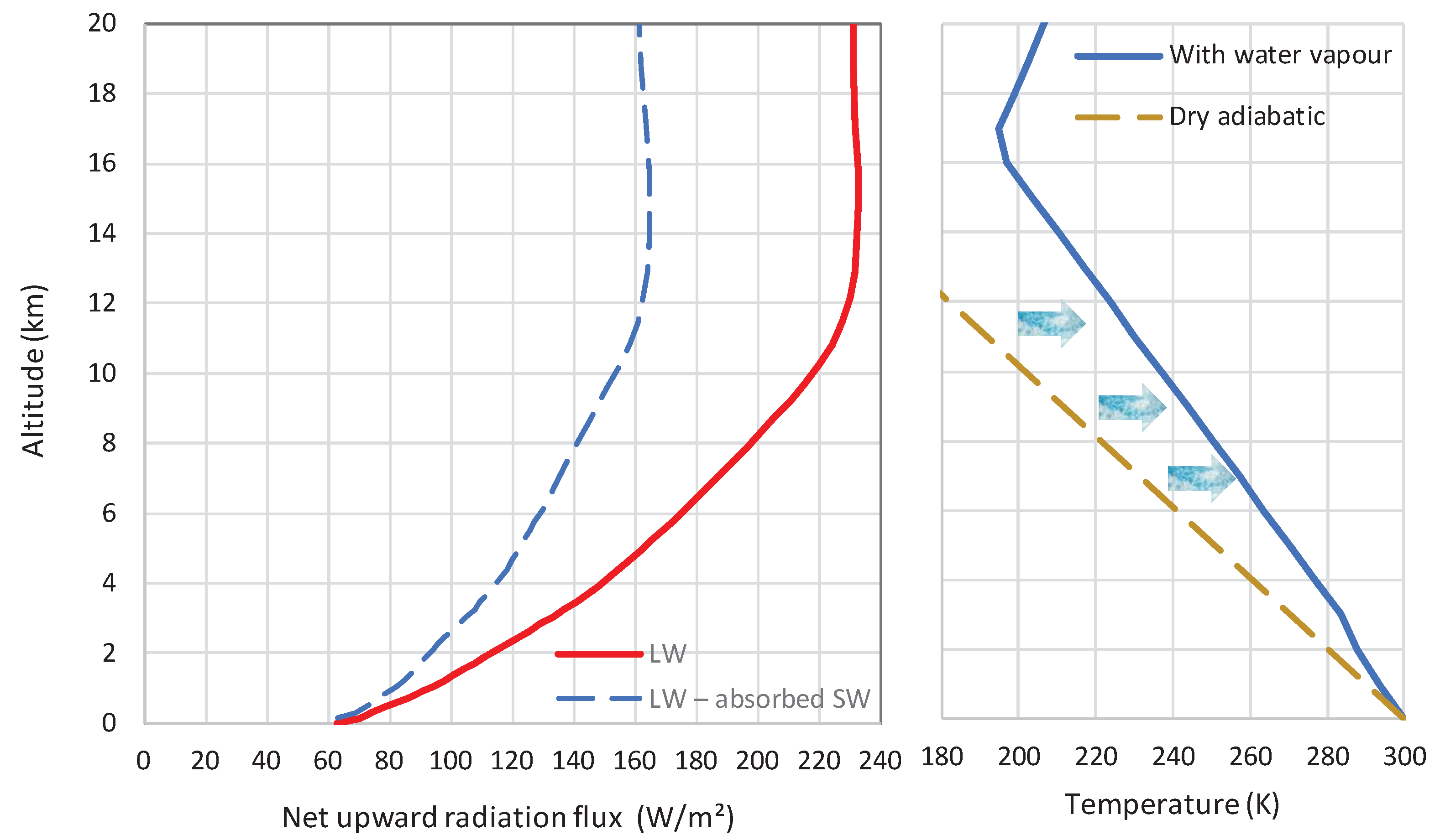
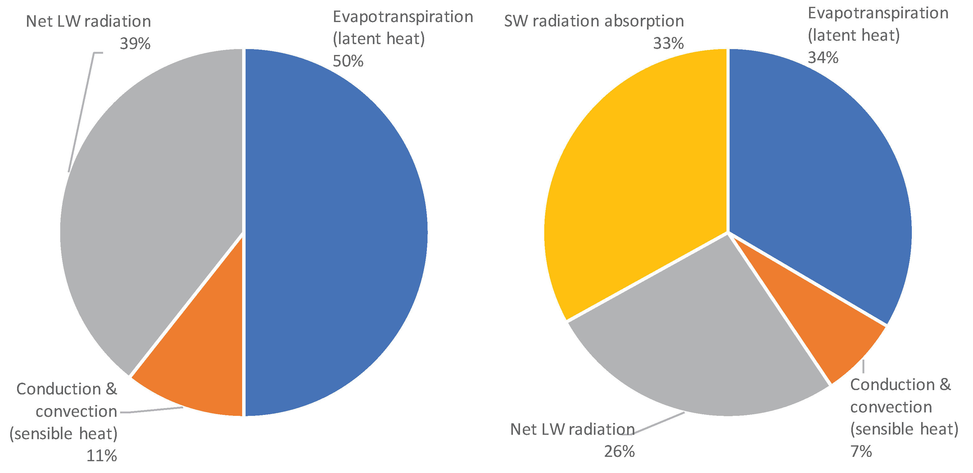
Surface cooling and atmosphere warming are reflected in the vertical profile of the net upgoing radiation flux, seen in Figure 25. Here the SW radiation was also considered, calculated by RRTM. The net radiation minus the absorbed SW radiation in the atmosphere is increasing with altitude. As, on the long term, the energy is not stored in the atmosphere, the total heat transfer should be the same at all altitudes. The deficit of heat transfer in low altitudes is recovered by sensible and latent heat transfer, which warm the atmosphere. Figure 26 shows diagrammatically the contribution of each of these mechanisms to Earth’s cooling and atmosphere’s warming.
Figure 25. (left) Vertical profile of net LW radiation flux for default conditions and standard tropical atmospheric profile (T = 299.7 K; [CO₂] = 400 ppm; L D = 369.26 W/m²; L O = 298.49 W/m²), as calculated by MODTRAN, and its difference from the net SW profile, as calculated by the RRTM Earth's Energy Budget (https://climatemodels.uchicago.edu/rrtm/). (right) MODTRAN’s standard tropical atmospheric profile of temperature, compared with the dry adiabatic profile (with a gradient of 9.8 K/km); the arrows indicated the heating of the atmosphere due to the latent heat released by condensation of water vapour, accumulated over elevation.
Preprints 103034 g025
Interestingly, heat exchange by evaporation (and hence the latent heat transfer from the Earth’s surface to the atmosphere) is the Earth’s natural locomotive, with the total energy involved in the hydrological cycle being 1290 ZJ/year, corresponding to an energy flux density of 80 W/m2. Compared to human energy production, the total energy of the natural locomotive is 2100 times higher than that of the human locomotive [10].
In addition to regulating the LW radiation flux and the latent heat flux, water vapour and clouds also regulate the SW radiation and Earth’s albedo. Other properties of water, as listed in Koutsoyiannis [10], are also determinant for climate. First is its unique property to appear on Earth in all three phases and in different formations, with spectacular differences among them in properties related to climate. Remarkable is its abundance on Earth, as only the part that is in turbulent motion amounts to 1.34 × 10⁹ Gt (not counting quantities that are stored in the soil, ground and glaciers), 260 times larger than the total mass of the atmosphere. The turbulent motion of water, which is intrinsically uncertain, generates climatic phenomena at all scales, from large-scale coupled ocean–atmosphere fluctuations, such as the El Niño–Southern Oscillation (ENSO), Atlantic Multidecadal Oscillation (AMO) and Interdecadal Pacific Oscillation (IPO), to regional droughts and floods. The high specific heat (or heat capacity) of water, particularly in its liquid phase, combined with its abundance, makes water the climatic thermostat of the Earth, i.e., the element that determines the heat storage and through it the climate of the Earth. The high specific latent heat of vaporization (calculated from Equation (6)) combined with the water occurrence on Earth in all three phases, makes water the thermodynamic regulator of climate. Finally, the fact that water is a universal solvent makes it an elixir of life, complementary to the CO₂ which is the other elixir of life, as through the photosynthesis it is responsible for the organic matter on which life on Earth is based.
Thus, the biosphere strongly depends on both CO₂ and H₂O. In particular, the presence of water determines the type and extent of ecosystems. In turn, the ecosystems affect climate at large through the carbon and oxygen cycles (where the vast majority of the CO₂ and O₂ emissions are products of life, through respiration and photosynthesis, respectively), and their contribution in the water cycle (transpiration) and in the energy cycle (photosynthesis). Humans, as part of the biosphere, also interact with water and climate, affecting them and being affected by them. Excluding human influences, the processes of the biosphere determine the vast majority (96%) of CO₂ emissions and partly, in the terrestrial part, the emission of H₂O by the transpiration process. And as Koutsoyiannis et al. [12,13] have shown, it is the relationship between temperature and biosphere that has determined the recent increase in the atmospheric [CO₂].
Considering all these facts, it is stunning that the whole “climate project”, including climate modelling, is based on hypotheses and scenarios about human CO₂ emissions.

8. Conclusions

According to the calculations presented here and the depiction of the results in Figure 24, the contribution of CO₂ to the greenhouse effect is 4% – 5%. Of this, 4% is due to human emissions, which means that the total human contribution on the enhancement of the greenhouse effect is 0.16% – 0.20% —a negligible effect. Irrespective of the origin of the increase of [CO₂] in the last century, its contribution to the greenhouse effect is about 0.5%, below any threshold to make it observable. In contrast, water (including clouds) contributes to the atmospheric greenhouse effect by 87% – 95%. In addition, 50% of Earth’s cooling and atmosphere’s warming is due to water (against 39% due to LW radiation, which again is dominated by water—Figure 26).
Common arguments trying to amplify the importance of human carbon emissions are that these accumulate to the atmosphere and that they cause temperature increase. The former argument is mistaken as the atmosphere does not have any mechanism to separate the incoming CO₂ according to its origin, and to accumulate that part that comes from humans. Also, the second argument has been refuted by showing, using modern instrumental CO₂ and temperature time series, that temperature changes precede CO₂ changes and thus the CO₂ increase cannot be a cause of the temperature increase [11,12,13,77].
Given these facts, the case of the magnified importance of CO₂, and particularly the human emissions thereof, appears to be a historical accident in scientific terms, that was exploited in non-scientific terms. If we return to science, the proper path is to improve hydrology and stochastics in order to better understand climate. For climate is mostly hydrology in terms of its driving physical mechanisms (as articulated here) and mostly stochastics in terms of its proper mathematical representation (as implied by its very definition; cf. Koutsoyiannis 2021, 2023).

Funding

This research received no funding but was conducted for scientific curiosity.

Data Availability Statement

This research uses no new data. The data sets used have been retrieved from the sources described in detail in the text.

Acknowledgments

I thank an anonymous reviewer of a predecessor paper [18], whose critical comments made it necessary to delve into the topic examined in the present paper. The brief reply to those review comments was not included in the predecessor paper in order not to distract its focus. Yet it constituted the springboard to produce this paper.

Conflicts of Interest

The author declares no conflicts of interest.

Appendix A: MODTRAN locality profiles

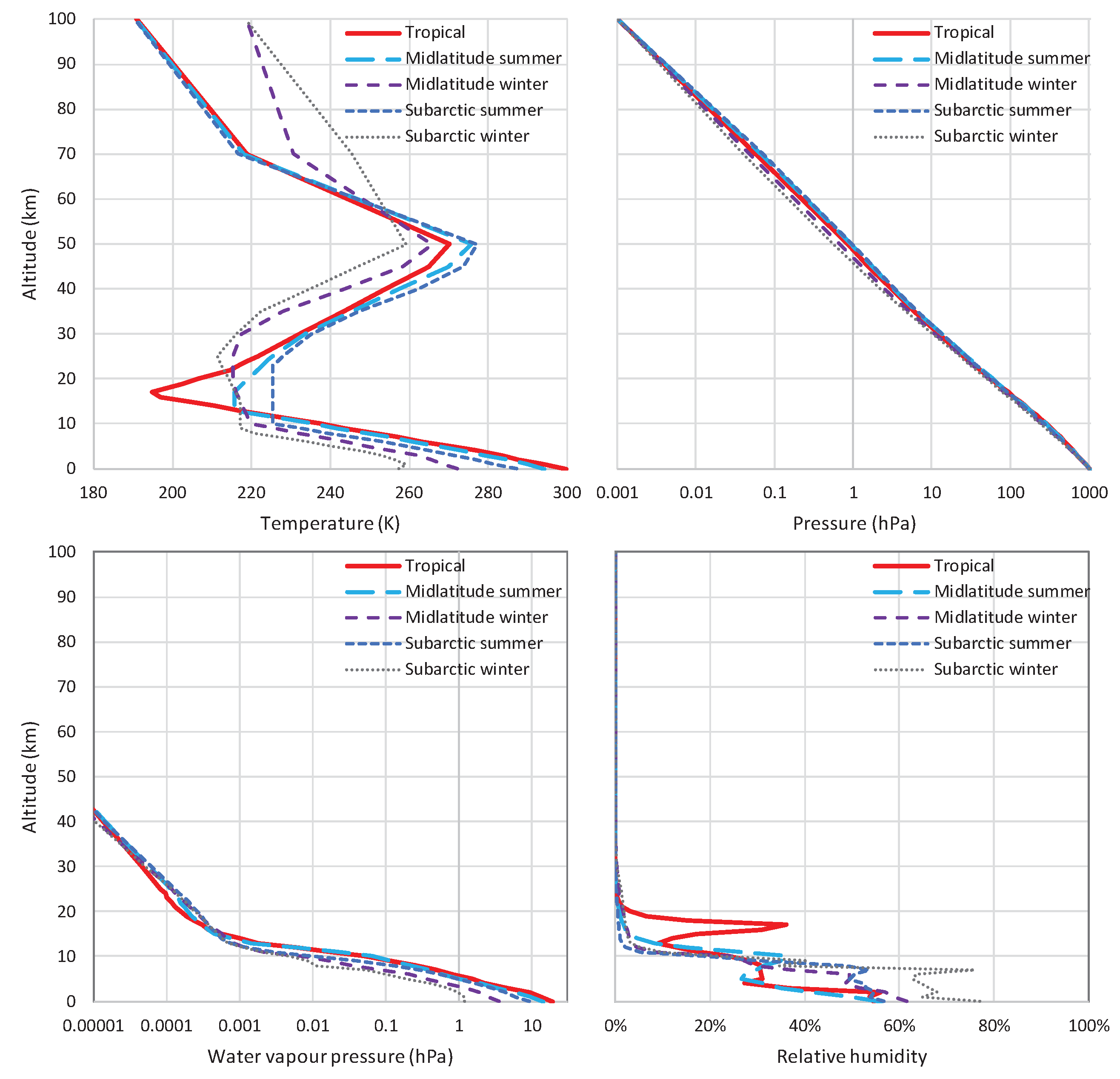
MODTRAN implements five different locality profiles, which differ in their temperature, H₂O and O₃ profiles. The profiles most relevant for this study are depicted Figure A1. (Additional information can be found in [78].) By comparison with zonal temperature distributions analogous to that of in Figure 4, but separately for summer and winter, we infer that the tropical profile corresponds roughly to the equator, but is representative for the entire torrid zone (between 23.4° N or S), the midlatitude profile corresponds to a latitude at about 45° N or S, and the subarctic profile at about the latitude of polar circles (66.6° N or S). In addition, MODTRAN includes the 1976 U.S. Standard Atmosphere temperature profile, which provides an effective median for the set of locality profiles; this was not used in this study.
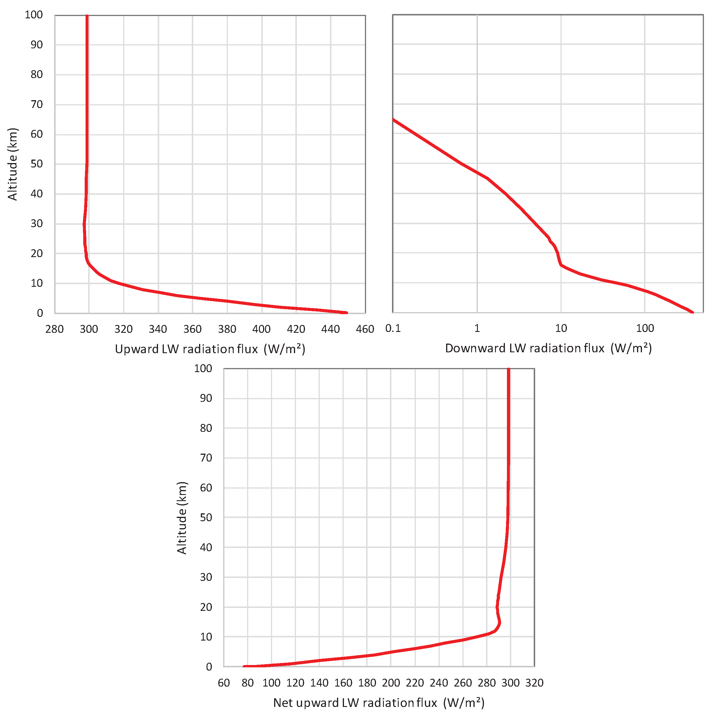
Figure A2 depicts a characteristic example of MODTRAN output profiles upward, downward and net LW radiation flux across the atmosphere for the tropical profile and default settings.
Figure A1. Standard profiles of the indicated variables used in MODTRAN.
Preprints 103034 g0a1
Figure A2. Profiles of the indicated variables resulting from MODTRAN for the tropical profile and default settings.
Preprints 103034 g0a2

References

  1. Searle, J.R. Minds, Brains and Science; Harvard University Press: Cambridge, MA, USA, 1984. [Google Scholar]
  2. Koutsoyiannis, D.; Mamassis, N. From mythology to science: the development of scientific hydrological concepts in the Greek antiquity and its relevance to modern hydrology. Hydrol. Earth Syst. Sci. 2021, 25, 2419–2444. [Google Scholar] [CrossRef]
  3. Koutsoyiannis, D. Rebuttal to review comments on “Revisiting global hydrological cycle: Is it intensifying?”. Hydrol. Earth Syst. Sci. Discuss. 2020. Available online: https://hess.copernicus.org/preprints/hess-2020-120/hess-2020-120-AC1-supplement.pdf (accessed on 13 February 2022). [CrossRef]
  4. Biermann, F.; Abbott, K.; Andresen, S.; Bäckstrand, K.; Bernstein, S.; Betsill, M.M.; Bulkeley, H.; Cashore, B.; Clapp, J.; Folke, C.; et al. Navigating the Anthropocene: Improving Earth System Governance. Science 2012, 335, 1306–1307. [Google Scholar] [CrossRef] [PubMed]
  5. Nature, Editorial Values Statement. https://www.nature.com/nature/editorial-values-statement (accessed on 27 March 2024).
  6. . Howe, N. ‘Stick to the science’: when science gets political. Nature 2020. [Google Scholar] [CrossRef]
  7. Nature Editorial. Should Nature endorse political candidates? Yes — when the occasion demands it. Nature 2023, 615, 561. [Google Scholar] [CrossRef] [PubMed]
  8. Lupia, A. Political endorsements can affect scientific credibility. Nature 2023, 615, 590–591. [Google Scholar] [CrossRef] [PubMed]
  9. Zhang, F.J. Political endorsement by Nature and trust in scientific expertise during COVID-19. Nature Human Behaviour 2023, 7, 696–706. [Google Scholar] [CrossRef]
  10. Koutsoyiannis, D. Rethinking climate, climate change, and their relationship with water. Water 2021, 13, 849. [Google Scholar] [CrossRef]
  11. Koutsoyiannis, D.; Onof, C.; Christofides, A.; Kundzewicz, Z.W. Revisiting causality using stochastics: 1. Theory. Proc. R. Soc. A 2022, 478, 20210836. [Google Scholar] [CrossRef]
  12. Koutsoyiannis, D.; Onof, C.; Christofides, A.; Kundzewicz, Z.W. Revisiting causality using stochastics: 2. Applications. Proc. R. Soc. A 2022, 478, 20210836. [Google Scholar] [CrossRef]
  13. Koutsoyiannis, D.; Onof, C.; Kundzewicz, Z.W.; Christofides, A. On hens, eggs, temperatures and CO2: Causal links in earth’s atmosphere. Sci 2023, 5, 35. [Google Scholar] [CrossRef]
  14. What is the greenhouse effect? – Climate Change: Vital Signs of the Planet. https://climate.nasa.gov/faq/19/what-is-the-greenhouse-effect/ (accessed on 20 October 2023).
  15. Greenhouse gas, Britannica. Available online: https://www.britannica.com/science/greenhouse-gas (accessed on 20 October 2023).
  16. Greenhouse effect, Britannica. Available online: https://www.britannica.com/science/greenhouse-effect (accessed on 20 October 2023).
  17. Lacis, A.A.; Schmidt, G.A.; Rind, D.; Ruedy, R.A. Atmospheric CO2: Principal control knob governing Earth’s temperature. Science 2010, 330, 356–359. [Google Scholar] [CrossRef]
  18. Koutsoyiannis, D.; Vournas, C. Revisiting the greenhouse effect—a hydrological perspective. Hydrol. Sci. J. 2024, 69, 151–164. [Google Scholar] [CrossRef]
  19. Nikolov, N.; Zeller, K. New insights on the physical nature of the atmospheric greenhouse effect deduced from an empirical planetary temperature. Model. Environ. Pollut. Climate Change 2017, 1, 1000112. [Google Scholar] [CrossRef]
  20. Miskolczi, F. Greenhouse gas theories and observed radiative properties of the Earth’s atmosphere. Sci. Clim. Change 2023, 3, 232–289. [Google Scholar] [CrossRef]
  21. Peachey, B. Mitigating human enhanced water emission impacts on climate change. In 2006 IEEE EIC Climate Change Conference; 2006. [Google Scholar] [CrossRef]
  22. Koutsoyiannis, D. Revisiting the global hydrological cycle: is it intensifying? Hydrol. Earth Syst. Sci. 2020, 24, 3899–3932. [Google Scholar] [CrossRef]
  23. Water use – AQUASTAT - FAO's Global Information System on Water and Agriculture. Available online: https://www.fao.org/aquastat/en/overview/methodology/water-use (last access: 19 February 2024).
  24. Masson-Delmotte, V.; Zhai, P.; Pirani, A.; Connors, S.L.; Péan, C.; Berger, S.; Caud, N.; Chen, Y.; Goldfarb, L.; Gomis, M.I.; et al. (Eds.) IPCC, Climate Change 2021: The Physical Science Basis. Contribution of Working Group I to the Sixth Assessment Report of the Intergovernmental Panel on Climate Change; Cambridge University Press: Cambridge, UK; New York, NY, USA, 2021; 2391p. [Google Scholar]
  25. UNESCO (United Nations Educational, Scientific and Cultural Organization). Final Report, International Hydrological Decade, Intergovernmental Meeting of Experts, UNESCO/NS/188; UNESCO House: Paris, 1964; Available online: https://unesdoc.unesco.org/images/0001/000170/017099EB.pdf (accessed on 15 February 2024).
  26. Koutsoyiannis, D. Clausius-Clapeyron equation and saturation vapour pressure: simple theory reconciled with practice. Eur. J. Phys. 2012, 33, 295–305. [Google Scholar] [CrossRef]
  27. Koutsoyiannis, D. Entropy: from thermodynamics to hydrology. Entropy 2014, 16, 1287–1314. [Google Scholar] [CrossRef]
  28. Koutsoyiannis, D. Stochastics of Hydroclimatic Extremes – A Cool Look at Risk, Edition 3; Kallipos Open Academic Editions: Athens, 2023; 391 pp. [Google Scholar] [CrossRef]
  29. Ambaum, M.H.P. Accurate, simple equation for saturated vapour pressure over water and ice. Q. J. R. Meteorol. Soc. 2020, 146, 4252–4258. [Google Scholar] [CrossRef]
  30. Murphy, D.M.; Koop, T. Review of the vapour pressures of ice and supercooled water for atmospheric applications. Q. J. R. Meteorol. Soc. 2005, 131, 1539–1565. [Google Scholar] [CrossRef]
  31. Goody, R.M. Atmospheric Radiation; Oxford University Press: Oxford, UK; New York, NY, USA, 1964; 436 pp. [Google Scholar]
  32. Brutsaert, W. On a derivable formula for long-wave radiation from clear skies. Water Resour. Res. 1975, 11, 742–744. [Google Scholar] [CrossRef]
  33. Prata, A.J. A new long-wave formula for estimating downward clear-sky radiation at the surface. Q. J. R. Meteorol. Soc. 1996, 122, 1127–1151. [Google Scholar]
  34. Brunt, D. Notes on radiation in the atmosphere. I. Q. J. R. Meteorol. Soc. 1932, 58, 389–420. [Google Scholar] [CrossRef]
  35. Brunt, D. Physical and Dynamical Meteorology; Cambridge University Press: Cambridge, UK, 1934; 411 pp, Available online: https://archive.org/details/in.ernet.dli.2015.215092 (accessed on 25 August 2023).
  36. Penman, H.L. Natural evaporation from open water, bare soil and grass. Proc. R. Soc. Lond. A Math. Phys. Eng. Sci. 1948, 193, 120–145. [Google Scholar]
  37. Monteith, J.L. Evaporation and environment. Symposia of the Society for Experimental Biology 1965, 19, 205–234. [Google Scholar] [PubMed]
  38. Doorenbos, J.; Pruitt, W.O. Guidelines for Predicting Crop Water Requirements. FAO Irrigation and Drainage Paper 24, Food and Agriculture Organization of the United Nations, Rome. 1977. Available online: https://dokumen.tips/download/link/fao-irrigation-and-drainage-paper-24.html (accessed on 25 August 2023).
  39. Allen, R.G.; Pereira, L.S.; Raes, D.; Smith, M.; Crop Evapotranspiration – Guidelines for Computing Crop Water Requirements. FAO Irrigation and Drainage Paper 56, Food and Agriculture Organization of the United Nations, Rome. Available online: https://www.fao.org/3/X0490E/x0490e00.htm (accessed on 25 August 2023).
  40. Carmona, F.; Rivas, R.; Caselles, V. Estimation of daytime downward longwave radiation under clear and cloudy skies conditions over a sub-humid region. Theor. Appl. Climatol. 2014, 115, 281–295. [Google Scholar] [CrossRef]
  41. Guo, Y.; Cheng, J.; Liang, S. Comprehensive assessment of parameterization methods for estimating clear-sky surface downward longwave radiation. Theor. Appl. Climatol. 2019, 135, 1045–1058. [Google Scholar] [CrossRef]
  42. Wong, R.Y.; Tso, C.Y.; Jeong, S.Y.; Fu, S.C.; Chao, C.Y. Critical sky temperatures for passive radiative cooling. Renewable Energy 2023, 211, 214–226. [Google Scholar] [CrossRef]
  43. Berk, A.; Bernstein, L.S.; Robertson, D.C. MODTRAN: A Moderate Resolution Model for LOWTRAN, Scientific Report No. 1; Air Force Geophysics Laboratory, Air Force Systems Command, United States Air Force: Hanscom Air Force Base, Massachusetts, USA. Available online: https://apps.dtic.mil/sti/pdfs/ADA185384; Available online: https://apps.dtic.mil/sti/pdfs/ADA185384.pdf (accessed on 19 February 2024).
  44. Berk, A.; Conforti, P.; Kennett, R.; Perkins, T.; Hawes, F.; van den Bosch, J. MODTRAN6: A Major Upgrade of the MODTRAN Radiative Transfer Code Proc. Philipona, R.; Kräuchi, A.; Brocard, E. Solar and thermal radiation profiles and radiative forcing measured through the atmosphere. doi:10.1029/2012GL052087.SPIE 2014, 9088, 90880H. Geophys. Res. Lett. 2012, 39, L13806. [Google Scholar] [CrossRef]
  45. Berk, A.; Acharya, P.K.; Bernstein, L.S.; Anderson, G.P.; Lewis, P.; Chetwynd, J.H.; Hoke, M.L. Band model method for modeling atmospheric propagation at arbitrarily fine spectral resolution. U.S. Patent #7433806.
  46. MODTRAN Infrared Light in the Atmosphere. Available online: https://climatemodels.uchicago.edu/modtran/ (last access: 19 February 2024).
  47. MODTRAN Demo. Available online: http://modtran.spectral.com/modtran_home (last access: 19 February 2024).
  48. RRTM Earth's Energy Budget. Available online: https://climatemodels.uchicago.edu/rrtm/ (last access: 19 February 2024).
  49. Philipona, R.; Kräuchi, A.; Brocard, E. Solar and thermal radiation profiles and radiative forcing measured through the atmosphere. Geophys. Res. Lett. 2012, 39, L13806. [Google Scholar] [CrossRef]
  50. Wielicki, B.A.; Barkstrom, B.R.; Harrison, E.F.; Lee III, R.B.; Smith, G.L.; Cooper, J.E. Clouds and the Earth's Radiant Energy System (CERES): An Earth observing system experiment. Bull. Amer. Meteor. Soc. 1996, 77, 853–868. [Google Scholar] [CrossRef]
  51. Doelling, D.R.; Loeb, N.G.; Keyes, D.F.; Nordeen, M.L.; Morstad, D.; Nguyen, C.; Wielicki, B.A.; Young, D.F.; Sun, M. Geostationary enhanced temporal interpolation for CERES flux products. J. Atmos. Ocean. Technol. 2013, 30, 1072–1090. [Google Scholar] [CrossRef]
  52. Doelling, D.R.; Sun, M.; Nguyen, L.T.; Nordeen, M.L.; Haney, C.O.; Keyes, D.F.; Mlynczak, P.E. Advances in geostationary-derived longwave fluxes for the CERES synoptic (SYN1deg) product. J. Atmos. Ocean. Technol. 2016, 33, 503–521. [Google Scholar] [CrossRef]
  53. CERES_SSF1deg_Ed4.1 Subsetting and Browsing. Available online: https://ceres-tool.larc.nasa.gov/ord-tool/jsp/SSF1degEd41Selection.jsp (last access: 19 February 2024).
  54. Kato, S.; Rose, F.G.; Rutan, D.A.; Thorsen, T.E.; Loeb, N.G.; Doelling, D.R.; Huang, X.; Smith, W.L.; Su, W.; Ham, S.-H. Surface irradiances of Edition 4.0 Clouds and the Earth's Radiant Energy System (CERES) Energy Balanced and Filled (EBAF) data product. J. Clim. 2018, 31, 4501–4527. [Google Scholar] [CrossRef]
  55. Loeb, N.G.; Doelling, D.R.; Wang, H.; Su, W.; Nguyen, C.; Corbett, J.G.; Liang, L.; Mitrescu, C.; Rose, F.G.; Kato, S. Clouds and the Earth's Radiant Energy System (CERES) Energy Balanced and Filled (EBAF) Top-of-Atmosphere (TOA) Edition-4.0 Data Product. J. Clim. 2018, 31, 895–918. [Google Scholar] [CrossRef]
  56. CERES_EBAF_Ed4.2 Subsetting and Browsing. Available online: https://ceres-tool.larc.nasa.gov/ord-tool/jsp/EBAF42Selection.jsp (last access: 19 February 2024).
  57. CERES. CERES_SSF1deg_Hour/Day/Month_Ed4A Data Quality Summary, Version 2 (Updated 8/4/2023). Available online: https://ceres.larc.nasa.gov/documents/DQ_summaries/CERES_SSF1deg_Ed4A_DQS.pdf (accessed on 15 February 2024).
  58. CERES. CERES_EBAF_Ed4.1 Data Quality Summary, Version 3 (Updated 12/9/2021). Available online: https://ceres.larc.nasa.gov/documents/DQ_summaries/CERES_EBAF_Ed4.1_DQS.pdf (accessed on 15 February 2024).
  59. Climate Explorer. Available online: https://climexp.knmi.nl/ (last access: 19 February 2024).
  60. WRIT: Monthly Timeseries: NOAA Physical Sciences Laboratory. Available online: https://psl.noaa.gov/cgi-bin/data/atmoswrit/timeseries.pl (last access: 19 February 2024).
  61. Dooge, J.C. Looking for hydrologic laws. Water Resour. Res. 1986, 22, 46S–58S. [Google Scholar] [CrossRef]
  62. Dingman, S.L. Physical Hydrology; Prentice Hall: Upper Saddle River, New Jersey, USA, 1994. [Google Scholar]
  63. Jacobs, J.D. Radiation climate of Broughton Island. In Energy Budget Studies in Relation to Fast-Ice Breakup Processes in Davis Strait; Barry, R.G., Jacobs, J.D., Eds.; Inst. of Arctic and Alp. Res. Occas. Paper no. 26; University of Colorado: Boulder, USA, 1978; pp. 105–120. Available online: https://www.colorado.edu/instaar/node/963 (accessed on 13 February 2024).
  64. Lhomme, J.P.; Vacher, J.J.; Rocheteau, A. Estimating downward long-wave radiation on the Andean Altiplano. Agric. For. Meteorol. 2007, 145, 139–148. [Google Scholar] [CrossRef]
  65. Brutsaert, W. Evaporation into the Atmosphere: Theory, History and Applications; Springer Science & Business Media: Dordrecht, Netherlands, 1991; 299pp. [Google Scholar]
  66. Schmidt, G.A.; Ruedy, R.A.; Miller, R.L.; Lacis, A.A. Attribution of the present-day total greenhouse effect. J. Geophys. Res. 2010, 115, D20106. [Google Scholar] [CrossRef]
  67. Brooks, F.A. Atmospheric radiation and its reflection from the ground. J. Atmos. Sci. 1952, 9, 41–52. [Google Scholar] [CrossRef]
  68. Salby, M.L. Physics of the Atmosphere and Climate; Cambridge University Press: New York, NY, USA, 2012. [Google Scholar]
  69. van Wijngaarden, W.A.; Happer, W. Dependence of Earth's thermal radiation on five most abundant greenhouse gases. arXiv 2020, arXiv:2006.03098. Available online: https://arxiv.org/abs/2006.03098 (accessed 25 August 2023).
  70. de Lange, C.A.; Ferguson, J.D.; Happer, W.; van Wijngaarden, W.A. Nitrous oxide and climate. arXiv 2022, arXiv:2211.15780. Available online: https://arxiv.org/abs/2211.15780 (accessed on 25 August 2023). [Google Scholar]
  71. Gerhart, L.M.; Ward, J.K. Plant responses to low [CO2] of the past. New Phytol. 2010, 188, 674–695. [Google Scholar] [CrossRef] [PubMed]
  72. Chen, X.; Chen, T.; He, B.; Liu, S.; Zhou, S.; Shi, T. The global greening continues despite increased drought stress since 2000. Glob. Ecol. Conserv. 2024, 49, e02791. [Google Scholar] [CrossRef]
  73. Veizer, J. Celestial climate driver: a perspective from four billion years of the carbon cycle. Geoscience Canada 2005, 32, 13–28. [Google Scholar]
  74. Veizer, J. Celestial climate driver: a perspective from four billion years of carbon cycle. In 34th Int. Seminar on Nuclear War and Planetary Emergencies; World Scientific: Erice, Italy, 2006; pp. 117–144. [Google Scholar]
  75. Veizer, J. Planetary temperatures/climate across geological time scales. In International Seminar on Nuclear War and Planetary Emergencies—44th Session: The Role of Science in the Third Millennium; 2012; pp. 287–288. [Google Scholar]
  76. Trenberth, K.E.; Fasullo, J.T.; Kiehl, J. Earth's global energy budget. Bull. Am. Meteorol. Soc. 2009, 90, 311–324. [Google Scholar] [CrossRef]
  77. Koutsoyiannis, D.; Kundzewicz, Z.W. Atmospheric temperature and CO₂: Hen-or-egg causality? Sci 2020, 2, 72. [Google Scholar] [CrossRef]
  78. The 6 model atmospheres in MODTRAN. 19 February. Available online: http://modtran.spectral.com/static/modtran6/html/help_atmosphere_model.html (last access: 19 February 2024).
Figure 1. Output of the MODTRAN model for the standard tropical atmospheric profile, in comparison to the case that the standard [CO₂] of 400 ppm is replaced by that of 800 ppm. The outgoing radiation corresponds to the level of 100 km above the ground. The ground temperature is 299.7 K (26.55 °C) and the total outgoing LW flux is 298.52 W/m² for [CO₂] = 400 ppm and 295.129 W/m² for [CO₂] = 800 ppm (difference –3.36 W/m²). Graph generated from https://climatemodels.uchicago.edu/modtran/.
Preprints 103034 g001
Figure 2. Geographical distribution of outgoing LW radiation averaged over the period of 2000 – 2022 as given by the CERES data: (upper) all sky; (lower) clear sky. Data retrieved from https://ceres-tool.larc.nasa.gov/ord-tool/jsp/SSF1degEd41Selection.jsp; graph generated by https://climexp.knmi.nl.
Preprints 103034 g002
Figure 3. Geographical distribution of cloud area fraction averaged over the period of 2000 – 2022 as given by the CERES data. Data source and graph generation as in Figure 2.
Preprints 103034 g003
Figure 4. Zonal distribution of LW radiation averaged over the period of 2000 – 2022 as given by the CERES data: (upper) downwelling; (lower) outgoing; , the temperature zonal distribution, as given by ERA5 Reanalysis is also plotted. Radiation data retrieved from https://ceres-tool.larc.nasa.gov/ord-tool/jsp/SSF1degEd41Selection.jsp for outgoing and https://ceres-tool.larc.nasa.gov/ord-tool/jsp/EBAF42Selection.jsp for downwelling; temperature data retrieved from, and graph generated by, https://climexp.knmi.nl.
Preprints 103034 g004
Figure 5. Graphical depictions of the relative intensity of outgoing LW radiation averaged over the period of 2000 – 2022 as given by the CERES data, as a function of the latitude; (left) ratio of intensity at latitude φ (S or N) to that at the equator; (right) cumulative flux between latitudes φ S and φ N to the total outgoing radiation.
Preprints 103034 g005
Figure 6. Depiction of monthly variability of outgoing LW radiation, as given by the CERES data; each point is the monthly value, spatially averaged over a geographical zone of 15° latitude, during the period of 2000 – 2022; the zonal distributions (temporal averages for the entire period as in Figure 4) are also shown for each hemisphere (SH and NH).
Preprints 103034 g006
Figure 7. Changes in the downwelling LW radiation, L D , as calculated by MODTRAN, due to changes in temperature (converted to blackbody radiation, σ T 4 ), and (upper) water vapour pressure ( e a ) and (lower) carbon dioxide concentration ([CO₂]). The calculations were made for the tropical profile, no clouds and default other settings. For the upper graph it was assumed [CO₂] = 400 ppm and for the lower graph e a = 19 hPa. Notice that the scale of the vertical axis is linear in the upper graph (with range ±10% of the central value) and logarithmic in the lower graph (with range from half to twice the central value).
Preprints 103034 g007
Figure 8. As in Figure 7 but for the outgoing LW radiation, L O .
Preprints 103034 g008
Figure 9. Comparison of downwelling LW radiation flux, L D , as computed by MODTRAN and by Equation (21).
Preprints 103034 g009
Figure 10. Comparison of outgoing LW radiation flux, L O , as computed by MODTRAN and by Equation (21).
Preprints 103034 g010
Figure 11. Comparison of outgoing LW radiation flux, L O , as computed by MODTRAN and by Equation (22), based on the downwelling flux, L D .
Preprints 103034 g011
Figure 12. Comparison of outgoing LW radiation flux, L O , as computed from MODTRAN and from Equation (21), fitted only for the tropical profile and for T = 299.7 ± 2 K, e a = 19 ± 1.9 hPa, and [CO₂] range of 200 – 800 ppm. The parameters of Equation (21) were reoptimized for these ranges, and the values T * = 56.2 K and e a * = 0.00683 hPa were found, while all others remained the same as in Table 1. The case of cumulus clouds is also plotted in the graph, with abscissae as derived by MODTRAN and ordinates equal to the values of Equation (21) for clear sky multiplied by 0.904.
Preprints 103034 g012
Figure 13. Effect of clouds to outgoing radiation, expressed as 1 L O A S / L O C S , i.e. the deviation from 1 of the ratio of longwave radiation for all sky ( L O A S ) to that for clear sky ( L O C S ), vs. the cloud fraction, C. The slopes of homogenous linear regressions, a C are also shown. Each plotted point corresponds to one of the 64 800 grid points of the CERES grids of clear-sky and all-sky radiation (Figure 2), and cloud area fraction (Figure 3), where the average over the period 2001-2022 was taken.
Preprints 103034 g013
Figure 14. Comparison of LW radiation components calculated by MODTRAN to radiosonde measurements by Philipona et al. [49].
Preprints 103034 g014
Figure 15. Comparison of emissivity calculated by MODTRAN to that calculated by Equation (21).
Preprints 103034 g015
Figure 16. Comparison of emissivity calculated by MODTRAN to that calculated by each of the indicated formulae; the explained variance (EV) is also shown for each case.
Preprints 103034 g016
Figure 17. Downwelling LW radiation flux vs. temperature, as calculated by MODTRAN for the five indicated locality profiles and default settings (points with crosses) as well as with temperature offsets from the default values of up to ±25 K (all other points), in comparison to the CERES EBAF zonal distribution shown in Figure 4.
Preprints 103034 g017
Figure 18. Outgoing LW radiation flux vs. temperature, as calculated by MODTRAN for the five indicated locality profiles and default settings (points with crosses) as well as with temperature departing from the default values by up to ±25 K (all other points), in comparison to the observed zonal distribution (CERES SSF1) as shown in Figure 4 and Figure 6.
Preprints 103034 g018
Figure 19. Time series of the indicated variables, averaged over the torrid zone. The values plotted are monthly averages, while the 11-year averages are also plotted in thicker lines.
Preprints 103034 g019
Figure 20. (upper) Time series of outgoing clear-sky LW radiation flux, averaged over the torrid zone, as given by CERES data and as predicted by Equation (21) with temperature, water vapour and [CO₂] data from the ERA5 and NCEP/NCAR Reanalyses. (lower) Time series outgoing all-sky LW radiation flux, averaged over the torrid zone, as given by CERES data and as predicted by the CERES clear-sky data and Equation (21) with CERES cloud area fraction. The values plotted are monthly averages, while the 11-year averages are also plotted in thicker lines.
Preprints 103034 g020
Figure 21. Output of the MODTRAN model, with the red curves in both panels produced for default settings (for the standard tropical atmospheric profile; T = 299.7 K; [CO₂] = 400 ppm; L O = 298.49 W/m²), and the blue curves produced for zero concentrations of all greenhouse gases except water vapour, assuming constant relative humidity and conditions such as to much the total outgoing LW flux of the red curves, namely: (left) temperature lower than default by 15 K (T = 284.7 K); (right) temperature equal to the default (T = 299.7 K) but water vapour scale increased to 1.3, accompanied by cumulus clouds.
Preprints 103034 g021
Figure 22. Difference of LW radiation flux from the values at the default settings of the standard tropical atmospheric profile (T = 299.7 K; [CO₂] = 400 ppm; L D = 369.26 W/m²; L O = 298.49 W/m²), as calculated by MODTRAN for the cases of (left) zero concentrations of all greenhouse gases except water vapour, assuming constant relative humidity and (right) as left but with [CO₂] = 200 ppm.
Preprints 103034 g022
Figure 23. Difference of LW radiation flux for the indicated conditions of [CO₂] from the respective values at the default settings of the standard tropical atmospheric profile (T = 299.7 K; [CO₂] = 400 ppm; L D = 369.26 W/m²; L O = 298.49 W/m²), as calculated by MODTRAN.
Preprints 103034 g023
Figure 24. Contribution of the greenhouse drivers to the LW radiation fluxes, (left) downwelling and (right) outgoing.
Preprints 103034 g024
Figure 26. Contribution of (left) the three mechanisms responsible for the cooling of Earth’s surface and (right) the four mechanisms responsible for the warming of Earth’s atmosphere, based on the energy balance by Trenberth et al. [76].
Preprints 103034 g026
Table 1. Fitted parameters of Equation (21) for ranges of temperature 247.2 – 309.7 K (–26.0 – 36.6 °C), water vapour pressure 1.08 – 20.9 hPa and CO₂ concentration 200 – 800 ppm.
Sign L * (W/m²) T * (K) e a * (hPa) C O 2 0 (ppm) η Τ η e a C O a C §
Downwelling ,   L D + 27 181 6.36 400 4.5 1 0.015 0.34
Outgoing ,   L O 1 55 0.00302 400 3.5 0.5 0.015 0.15
Specific sign to replace ± in Equation (21). § These are global values; for values of outgoing radiation per geographical zone see Figure 13. Not necessary to optimize.
Table 2. Performance indices of Equations (21) (with parameters as in Table 1) and (22), fitted for ranges of temperature 247.2 – 309.7 K (–26.0 – 36.6 °C), water vapour pressure 1.08 – 20.9 hPa and CO₂ concentration 200 – 800 ppm, and clear sky.
Equation, variable Range   of   L (W/m2) RMSE   in   L (W/m2) Explained   variance §   of   L (%) RMSE   in   relative   error   ( L e L / L (%) Maximum   absolute   relative   error   | L e L | / L (%)
( 21 ) ,   downwelling ,   L D 140.0 – 419.5 1.3 99.97 0.5 1.9
( 21 ) ,   outgoing ,   L O 170.6 – 351.1 1.3 99.79 0.7 1.9
(22) ,   outgoing ,   L O   from   L D 170.6 – 351.1 3.6 99.24 1.5 4.5
Root mean square error. § Also known as Nash-Sutcliffe performance index.
Table 3. Ratios of outgoing LW radiation under cloudy sky to that for clear sky, for the indicated types of clouds and locality profiles, as determined by MODTRAN for default settings (the lowest value is highlighted in bold).
Locality profile
    →
Cloud type ↓
Tropical Midlatitude summer Subarctic summer Midlatitude winter Subarctic winter
Cumulus 0.904 0.899 0.889 0.910 0.95
Altostratus 0.901 0.896 0.887 0.907 0.948
Stratus 0.966 0.973 0.962 0.973 1.016
Stratus/Stratocumulus 0.939 0.945 0.931 0.950 0.989
Nimbostratus 0.98 0.984 0.977 0.984 1.024
Standard Cirrus 0.93 0.939 0.957 0.95 0.974
NOAA Cirrus 0.937 0.945 0.963 0.956 0.98
Table 4. Comparison of observed data and MODTRAN results for the average conditions of each of the indicated two periods. The observed data are global averages. The MODTRAN results are for the average observed temperature and [CO₂] of each period, and for the same water vapour scales in the two periods, estimated so as to (approximately) match the outgoing clear-sky LW flux of CERES for the first period, while holding fixed relative humidity for the two periods.
Period → 2001-11 2012-22 Difference
Observations (averages over each period)
Temperature from ERA5 (K) 287.21 287.49 +0.28
[CO₂] from Mauna Loa (ppm) 381.83 406.48 +24.65
Outgoing TOA (20 km) clear-sky LW from CERES (W/m2) 268.33 268.27 –0.08
Outgoing clear-sky LW radiation by MODTRAN at 20 km altitude (W/m2)
Tropical profile, water vapour scale 0.82 268.34 268.72 +0.38
Midlatitude summer profile, water vapour scale 1.08 268.34 268.78 +0.44
Midlatitude winter profile, water vapour scale 1.14 268.28 268.78 +0.50
Subarctic summer profile, water vapour scale 2.56 268.31 268.91 +0.60
Table 5. Results of MODTRAN calculations for temperature of 288 K (the value of current global temperature used by Brutsaert [32] and tropical profile and extreme (imaginary-world) cases of greenhouse gas concentrations.
[CO₂] relative to the default value of 400 ppm Water vapour scale relative to the default tropical profile Other greenhouse gases concentration relative to default Downward IR heat flux at surface (W/m²) Upward IR heat flux at surface (W/m²) Outgoing LW radiation flux at 100 km altitude (W/m²)
1 1 1 325.6 381.5 249.5
1 1 0 324.0 381.5 256.7
0 0 0 1.7 380.3 379.0
1 0 0 68.2 380.3 340.7
2500* 0 0 215.7 381.5 257.1
0 0.0015 0 78.8 380.3 366.4
0 0.04 0 157.8 380.6 340.7
0 0.2 0 212.5 380.9 319.3
0 1 0 319.7 381.5 284.7
0 2.2 0 372.1 381.8 257.7
* In this case the atmosphere is composed merely by CO₂ (2500 × 400 = 1 000 000 ppm = 1).
Table 6. Relative changes of LW radiation fluxes at standard conditions, equal to the global averages, T = 288.6 K, e a = 15.2 hPa, C O 2 = 400 ppm, C = 0.671, as calculated analytically and numerically by Equation (21).
Case of relative change Relative change expression Numerical value of relative change
Downwelling flux Outgoing flux
L T # η Τ T T * η Τ 1 + T T * η Τ ± e a e a * η e 3.18 4.44
L e a # ± η e e a e a * η e 1 + T T * η Τ ± e a e a * η e 0.207 –0.136
L C O 2 # ± a C O 1 ± a C O ln C O 2 C O 2 0 0.015 –0.015
L C # ± a C C 1 ± a C C 0.186 –0.112
L A O # (see text) 0.006 –0.023
Table 7. Relative changes of LW radiation fluxes at standard conditions, equal to the global averages, T = 288.6 K, e a = 15.2 hPa, C = 0.671 (or C = 0 for clear sky), and with the indicated values of [CO₂] as calculated analytically and numerically by Equation (21). In parentheses are the values directly calculated by MODTRAN assuming midlatitude summer profile matching the above values of T and e a , and altostratus clouds for the cloudy case.
[CO₂] increase Sky Downwelling ,   L D Outgoing ,   L D
Δ L D L D mean* % change Δ L O L D mean* % change
From 300 to 420 Cloudy 1.93
(0.31)
382.4
(374.1)
0.5%
(0.1%)
–1.18
(–1.00)
235.1
(238.0)
–0.5%
(–0.4%)
From 300 to 420 Clear 1.57
(0.79)
311.3
(309.6)
0.4%
(0.3%)
–1.32
(–1.32)
261.5
(265.7)
–0.5%
(–0.5%)
From 300 to 800 Cloudy 5.63
(0.63)
384.2
(374.3)
1.5%
(0.2%)
–3.45
(–2.89)
234.0
(237.0)
–1.5%
(–1.2%)
From 300 to 800 Clear 4.59
(2.45)
312.8
(310.5)
1.2%
(0.8%)
–3.84
(–3.89)
260.2
(264.4)
–1.5%
(–1.5%)
* Geometric mean.
Disclaimer/Publisher’s Note: The statements, opinions and data contained in all publications are solely those of the individual author(s) and contributor(s) and not of MDPI and/or the editor(s). MDPI and/or the editor(s) disclaim responsibility for any injury to people or property resulting from any ideas, methods, instructions or products referred to in the content.
Copyright: This open access article is published under a Creative Commons CC BY 4.0 license, which permit the free download, distribution, and reuse, provided that the author and preprint are cited in any reuse.
Prerpints.org logo

Preprints.org is a free preprint server supported by MDPI in Basel, Switzerland.

Subscribe

© 2024 MDPI (Basel, Switzerland) unless otherwise stated