Preprint

Article

Redundant Space Manipulator Autonomous Guidance for In-Orbit Servicing via Deep Reinforcement Learning

Altmetrics

Downloads

103

Views

Comments

A peer-reviewed article of this preprint also exists.

This version is not peer-reviewed

Submitted:

02 April 2024

Posted:

04 April 2024

You are already at the latest version

Alerts

Abstract

The application of space robotic manipulators and heightened autonomy for ios represents a paramount pursuit for leading space agencies, given the substantial threat posed by space debris to operational satellites and forthcoming space endeavors. This work presents a guidance algorithm based on drl to solve for the space manipulator path-planning during the motion synchronization phase with the mission target. The goal is the trajectory generation and control of a spacecraft equipped with a 7-dof robotic manipulator, such that its end effector remains stationary with respect to the target point of capture. The ppo drl algorithm is used to optimize the manipulator’s guidance law, and the autonomous agent generates the desired joints rates of the robotic arm, which are then integrated and passed to a model-based feedback linearization controller. The agent is first trained to optimize its guidance policy and then tested extensively to validate the results against a simulated environment representing the motion synchronization scenario of an ios mission.

Keywords:

Subject: Engineering - Aerospace Engineering

1. Introduction

The recent surging interest in advancing technologies and methodologies for IOS of satellites and space systems is motivated by the continuous expansion of space exploration and utilization, demanding for efficient and dependable approaches to repair, refuel, and reposition space assets. Spaceborne robotic systems are a key technology potentially unlocking the capability to perform these tasks, and their accurate handling and control is an essential aspect of IOS missions. The aforementioned activities are carried out either on a cooperative or an uncooperative target, and it is the latter scenario that is driving the current research field. The inherent uncertainties associated with the interaction with uncooperative targets necessitate a high degree of motion control autonomy, reactivity and adaptability to the surrounding environment. The rapid progress in the field of artificial intelligence is promising substantial enhancements in the capabilities of autonomous Guidance, Navigation, and Control (GNC) within these systems. Reinforcement Learning (RL), above all, seems like a promising tool to solve complex decision making problems, formulated as Markov Decision Processes (MDP). The fusion of Neural Networks’ generalization abilities with Reinforcement Learning methods has given rise to DRL, which is extensively employed in solving planning problems for its capacity to handle high dimensional state and action spaces, as well as the possibility to cope with Partially Observable Markov Decision Process (POMDP).

DRL has been recently adopted to generate the trajectory to fly around a target object for its autonomous shape reconstruction in [1] and [2]. Other applications of RL, and more specifically meta-RL, are applied in [3] to enhance the guidance and control of endoatmospheric missiles, in [4] for 6-DoF planetary landing applications, and in [5] for the autonomous generation of asteroid close-proximity guidance.

Regarding the application of RL to aid in space robot guidance and control, such methodology is currently considered one of the most promising research directions [6], but present literature is still quite scarce. Indeed, further research efforts in the short term will be required to unlock its full potential. In [7] a motion planning strategy for a 7-DoF space manipulator is implemented, and some of the concepts detailed in that work are also applied here, specifically in the context of the reward function. Multi-target trajectory planning is presented in [8], while control of a free-floating space robot through RL is tackled in [9].

The aim of this work is to take a step forward the application of DRL for the trajectory planning of a high-DoF space manipulator in a challenging and dynamical environment as the one of IOS missions. The obtained results demonstrate the enhanced autonomy and reactivity provided by the application of DRL in the context of the motion synchronization phase of an hypothetical IOS mission, and prove that the proposed method has the potential to be extended to a wider set of spaceborne scenarios.

2. Problem Statement

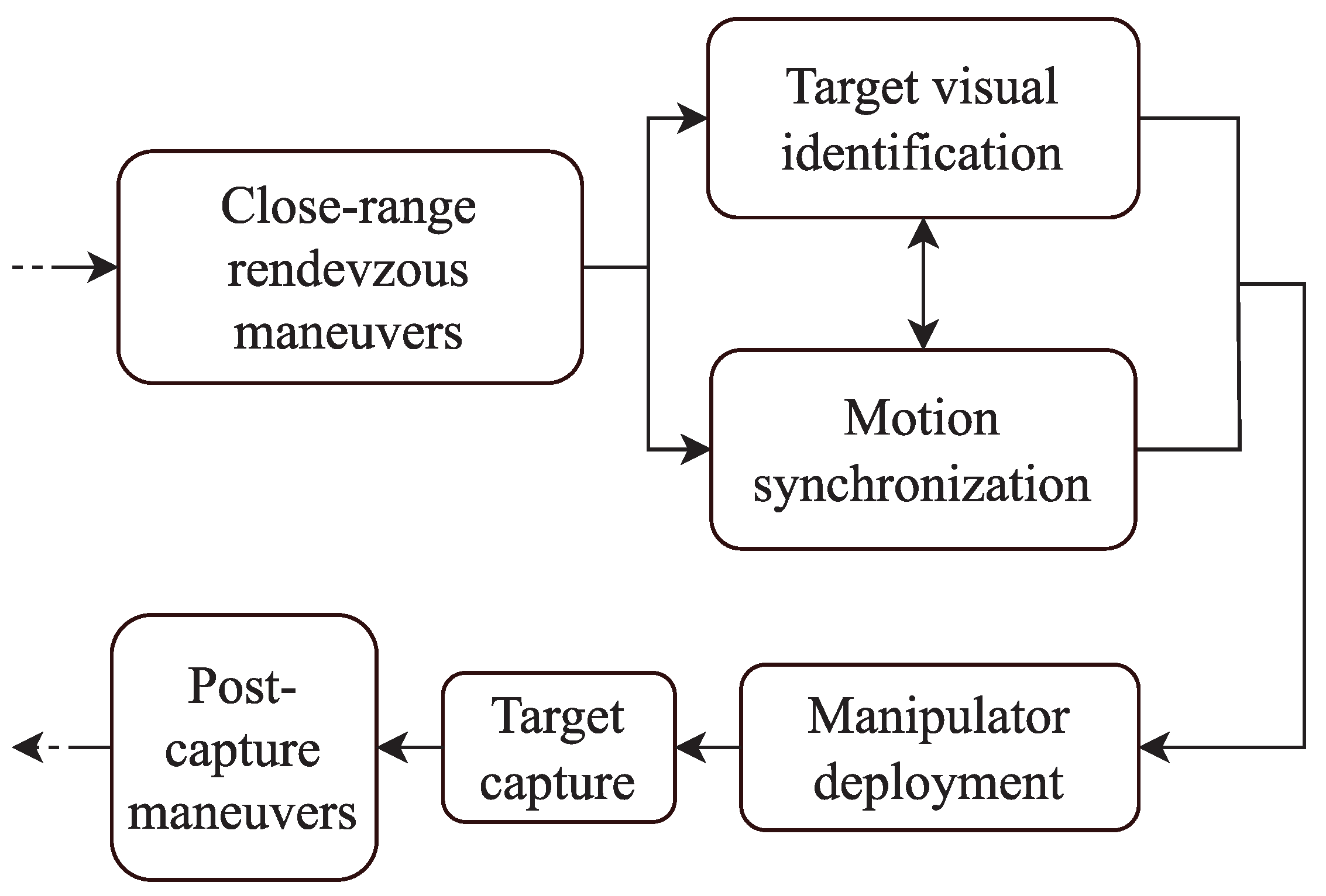
The case study that is being analyzed is now better defined. In robotic IOS missions, a key phase involves motion synchronization. The main operations performed during a robotic IOS mission are reported in a block diagram in Figure 1.

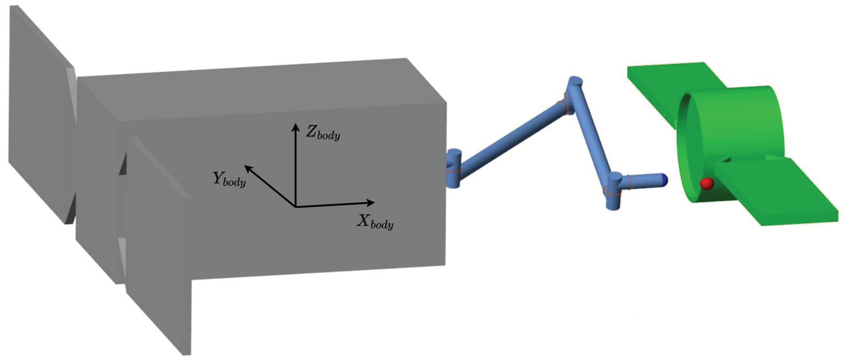
During this phase, the chaser spacecraft fine-tunes its relative position and angular orientation until its end effector remains stationary relative to the target capture point. Achieving the correct relative state at the end of this closing phase is critical for the subsequent tasks of grasping and making contact. Figure 2 illustrates the problem at hand.

The end effector of the space manipulator shall effectively track a specified grasping point on the tumbling target and follow its motion, in preparation to the subsequent activities. A generic shape for the target is selected, without loss of generality, and it is designed as a cylinder with two appendages representing solar panels. The chaser instead, is a 6-DoF spacecraft equipped with a 7-DoF redundant manipulator.

The DRL agent, that is PPO, performs the guidance and control tasks, receiving the input data from the navigation block. The work operates under the assumption of having prior knowledge of the state variables describing the scenario at every time instant, and omits the inclusion of a physical navigation block responsible for estimating these state parameters, since it is outside of the scope of this study.

Consequently, the state variables are presumed to be available and are directly input into the guidance and control blocks. These blocks then generate control actions, which are subsequently applied to the system. The system, in turn, integrates the equations of motion for both the chaser and the target and provides the scenario for the next simulation step, effectively closing the feedback loop.

2.1. Space Manipulator Dynamics

This section provides a concise introduction to the equations of motion for a space manipulator with N degrees-of-freedom. It’s important to note that, in the scope of this study, the multi-body system is described as free-flying, signifying that the spacecraft is actively controlled in both translation and rotation, in contrast to the free-floating scenario [10]. By employing the direct path approach, the spacecraft’s center of mass is utilized as the representative point for translational motion, enabling the derivation of the system’s kinematics and dynamics. This approach results in more streamlined equations. Using a Newton-Euler formulation, the equations of motion of the space manipulator system are computed, and they are reported in Equation (1).

H (q) \ddot{q} + C (q, \dot{q}) \dot{q} = τ

(1)

H \in R^{(6 + N) \times (6 + N)}

is the symmetric, positive -definite Generalized Inertia Matrix (GIM),

C \in R^{(6 + N) \times (6 + N)}

is the Convective Inertia Matrix (CIM), containing the nonlinear contributions, the Coriolis and centrifugal forces, and

τ \in R^{(6 + N)}

is the vector of generalized forces in the joint space. The parameter

q

entails the selected generalized variables, which compose the space manipulator state and are reported in Equation (2):

q = {[r_{0}, R_{0}, q_{m}]}^{⊤} = {[q_{0}, q_{m}]}^{⊤}

(2)

where

r_{0}

is the position vector of the base spacecraft in inertial frame,

R_{0}

is the orientation of the base spacecraft with respect to the inertial frame, employing a quaternion representation, and

q_{m}

contains the joint angles of the robotic arm.

The kinematic and dynamic properties of the system are determined using the MATLAB library SPART (SPAce Robotics Toolkit) [11], a software package designed for modeling and controlling mobile-base robotic multi-body systems with efficient and recursive algorithms, taking advantage of the kinematic tree topology of the system. Additionally, for solving the equations of motion, a model of the space manipulator is constructed using the Simulink Simscape Multi-body library.

2.2. Target Dynamics

As the target is positioned at the origin of the LVLH reference frame, its translational motion can be disregarded, focusing instead on the rotational dynamics, which is modeled using Euler equations in orthogonal principal axes of inertia coordinates, as in Equation (3).

I \dot{ω} + ω \times (I ω) = M

(3)

I

is the target inertia matrix,

ω

the angular velocity vector, and

M

is the vector of applied torques. Once again, the equations of motion of the target are solved through a Simulink Simscape Multi-body model of the target.

3. Reinforcement Learning Guidance

RL is a widely utilized tool for tackling MDPs. When combined with Neural Networks for function approximation, it becomes a potent method for addressing complex problems characterized by high-dimensionality and partial observability [12]. A cutting-edge DRL algorithm designed for problems with continuous state and action spaces, that is PPO [13], is investigated for the robotic manipulator’s guidance optimization.

3.1. Proximal Policy Optimization

PPO is a state-of-the-art on-policy, model-free DRL algorithm belonging to the family of policy-gradient methods. With respect to its predecessor Trust Region Policy Optimization (TRPO) [14], PPO provides a simper implementation with higher sample efficiency, which makes for faster training without compromising reliability. As for its performance on complex, high-dimensional, and partially observable continuous control problems, PPO outperforms many of its competitors in various benchmarks and provides high training stability. PPO is based on the Actor-Critic framework [15], where the actor represents the decision-making logic of the agent (i.e. the policy

π

), and the critic evaluates the actions of the actor in the environment. Both actor and critic are approximated through Deep Neural Networks (DNNs) parametrized through variables

θ

, which are updated throughout the training process. The Actor-Critic approach is briefly described:

An agent is initially situated at a state s, and perceives its environment through observations o.
Based on o, the actor autonomously decides the action a to take, and applies it in the environment to move to a new state $s^{'}$ .
Depending on the definition of the reward $R (a_{k}, s_{k})$ , the critic evaluates the action that has been taken, and guides the parameter updates of the actor through stochastic gradient descent on a loss function.

The optimal policy in an infinite-horizon problem is found through Equation (4), and provides the agent with the maximum reward when applied in the environment.

π^{*} = \underset{π}{argmax} E_{π} [\sum_{k = 0}^{\infty} γ^{k} R (a_{k}, s_{k})]

(4)

where the discount factor

γ \in [0, 1]

introduces a decay of rewards obtained distantly in time, and measures whether the agent seeks short-term or cumulative rewards.

Compared to the loss function in trpo, PPO’s clipped surrogate objective (Equations 5 and 6) has the advantage of limiting the policy’s parameter updates by clipping the loss function, providing increased training stability.

p_{k} (θ) = \frac{π_{θ} (a_{k} | s_{k})}{π_{θ_{o l d}} (a_{k} | s_{k})}

(5)

L^{C L I P} (θ) = E_{k} [m i n (p_{k} (θ), c l i p (p_{k} (θ), 1 - ε, 1 + ε))] A_{k}

(6)

where

A_{k}

(Equation (7)) is the advantage function at timestep k, and

ε

is the hyperparameter defining the clipping range. The entropy loss term

S (π_{θ}) s_{k}

, weighted by a hyperparameter w, is added to Equation (6) to promote agent exploration, and encourages the actor to try a variety of different actions, without becoming too greedy towards the ones it thinks are best. Finally, the advantage function (Equation (7)) measures how advantageous taking an action a at timestep k is, with respect to simply running the current policy

π_{θ}

. The critic’s job is to approximate the value function

V (s_{k})

, which represents the cumulative sum of discounted rewards if only the current policy were to be run until the end of the episode.

A (s_{k}, a_{k}) = [\sum_{j = k}^{T} γ^{j - k} R (a_{k}, s_{k})] - V (s_{k})

(7)

3.2. GNC Implementation and Environment

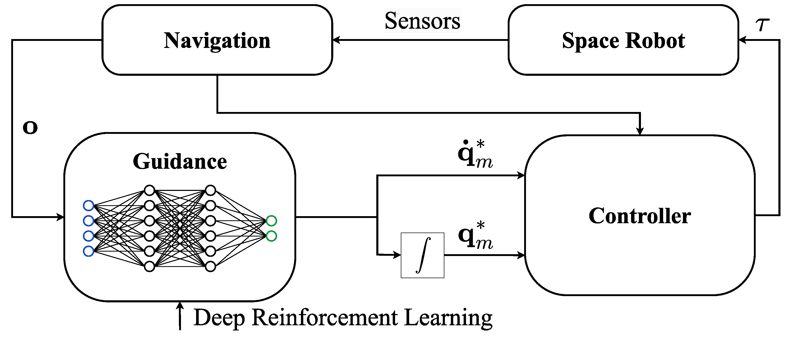
This work presents a novel Artificial Intelligence (AI)-based autonomous guidance law for a 7-DoF redundant manipulator mounted on a Space Robot (SR), used to achieve simultaneous end-effector positioning and attitude alignment with respect to a desired state, as well as its tracking. As defined in [12], the environment in the DRL framework corresponds to everything outside of the agent’s control, hence everything outside of the manipulator’s guidance system is taken as part of the environment, including the remainder of the SR and the target. A simplified scheme of the SR’s GNC system is reported in Figure 3.

The SR’s control system is implemented through a coupled, nonlinear model-based feedback linearization controller, where the resulting system is controlled through two Proportional-Derivative (PD) regulators, respectively for the base and manipulator. The base is kept at the desired synchronized state with respect to the target, while the manipulator is commanded by the DRL agent. The coupled control law is provided in Equation (8), but being part of the DRL environment, it could be substituted with a more performant control approach with little to no retraining.

\begin{matrix} τ = \{\begin{matrix} τ_{0} \\ τ_{m} \end{matrix}\} = H \{\begin{matrix} P D (q_{0}^{*} - q_{0}) \\ P D (q_{m}^{*} - q_{m}) \end{matrix}\} + C \dot{q} \end{matrix}

(8)

where

H

and

C

are respectively the system’s 13×13 GIM and CIM [11], and

q = {[q_{0}, q_{m}]}^{⊤}

collects the 6-DoF of the base and the 7-DoF of the manipulator. The scalar gains of the two PD are set as in Table 1, and have been tuned through trial-and-error.

3.3. Action Space and Observation Space

The agent’s policy, which represents the actor of the PPO implementation and provides autonomous guidance of the manipulator, receives 32 observations

o

(Equation (9)), and outputs 7 actions

a

(Equation (10)).

o = {[q_{m}, {\dot{q}}_{m}, \tilde{r}, \tilde{DCM}, \tilde{v}, \tilde{ω}]}^{⊤}

(9)

The terms in Equation (9) correspond to the current joint angles and joint rates of the manipulator, and the errors between the current and desired end-effector state, retrieved through kinematics, and rotated in the SR’s body frame. This vector is normalized before providing it to the guidance for better convergence of PPO [8]. The main benefit of using the agent only to provide manipulator guidance, is that kinematic information is sufficient in the observations, which decreases the complexity of the policy and eases convergence of the algorithm.

a = {\dot{q}}_{m}^{*} = {[{\dot{ϕ}}_{1}, {\dot{ϕ}}_{2}, {\dot{ϕ}}_{3}, {\dot{ϕ}}_{4}, {\dot{ϕ}}_{5}, {\dot{ϕ}}_{6}, {\dot{ϕ}}_{7}]}^{⊤}

(10)

The 7 actions produced by the agent correspond to the desired joint rates of the manipulator, and are integrated (Figure 3) such that both the desired joint angles and rates can be provided to the manipulator’s PD controller [16].

3.4. Reward

Providing the agent with rewards and penalties is the sole mechanism that incentivizes the manipulator’s guidance system to increase its performance. Adequate reward function design is critical as it directly impacts the convergence of the policy towards the optimal one, as well as the overall attainable performance. Since training on a sparse reward with high-dimensional state and action spaces is extremely difficult, reward shaping has been introduced through the definition of an Artificial Potential Field (APF)(Equation (11)), expanding upon [7].

U_{k} = - \tilde{r} + \frac{10}{1 + {\tilde{r}}_{a x}} + \frac{10}{1 + {\tilde{r}}_{t x}} + \frac{10}{1 + \tilde{θ}}

(11)

where

\tilde{r}

is the magnitude of the error between the desired and current positions of the end-effector,

{\tilde{r}}_{a x}

and

{\tilde{r}}_{t x}

are the projections of

\tilde{r}

parallel and transverse to the X-axis of the SR’s body frame (Figure 2), and

\tilde{θ}

is the scalar error angle between the desired and current attitude of the end-effector, in axis-angle representation. The reward is given as a function of the end-effector’s potential variation (

Δ U

) between timesteps (Equation (12) and 13).

\begin{matrix} Δ U = U_{k} - U_{k - 1} \end{matrix}

(12)

\begin{matrix} R_{k} = \{\begin{matrix} Δ U & if Δ U \geq 0 \\ 1.5 Δ U & if Δ U < 0 \end{matrix} \end{matrix}

(13)

where the

1.5 \times

multiplier discourages the end-effector from moving along equipotential surfaces. A bonus sparse reward of

+ 0.01

is provided while

{\tilde{r}}_{a x}

{\tilde{r}}_{t x}

, and

\tilde{θ}

are simultaneously below a desired threshold.

4. Training and Results

Before proceeding with training, the initial conditions and the DRL hyperparameters are introduced. The scenario is that of a target spacecraft tumbling around its major inertia axis. The SR’s state is kept synchronized with that of the target, such that they spin together and any relative motion between the desired end-effector state and the SR is minimized. The SR is positioned along the angular momentum (

L_{T}

) of the target at a nominal distance of 5 m, and its angular velocity is set as in Equation (14) for synchronization purposes.

ω_{0} = {[ω_{T} \cdot {\hat{L}}_{T}, 0, 0]}^{⊤}

(14)

The nominal initial manipulator state is found in Equation (15).

\begin{matrix} q_{m} = {[0, 285, 0, 210, 0, 75, 0]}^{⊤} \deg & {\dot{q}}_{m} = {[0, 0, 0, 0, 0, 0, 0]}^{⊤} \deg / s \end{matrix}

(15)

To increase the robustness of the agent, and to show that it can adapt to conditions that haven’t strictly been trained on, the nominal initial conditions of the target object and of the SR are randomized at the start of each simulation, according to the following list:

Target’s major-axis spin rate $ω_{T} \in [- 3, 3]$ deg/s.
Each initial manipulator joint angle is perturbed by a random value $δ ϕ_{i} \in [- 15, 15]$ deg.
Desired end-effector state is randomized on the whole SR-facing side of the target, both in terms of position and attitude.
Distance between SR and target is perturbed by a random value $δ d \in [- 25, 25]$ cm.

Simulations are only terminated if the manipulator’s configuration becomes singular, to prevent the DRL algorithm from breaking down due to mathematical issues. With regards to the PPO hyperparameters, the sample time of the agent is set to

0.3

s as a trade-off between computational expense, convergence, and reactivity of the SR. The actor and critic are represented through two Feedforward Neural Networks (FNNs), with hyperparameters in Table 2.

A stochastic policy is used to increase agent exploration [9], hence the actor’s 14 outputs (Table 2) represent respectively the mean and standard deviation of each desired joint velocity. The remainder of the PPO hyperparameters are selected among typical values: the clipping factor

ε = 0.2

, the discount factor

γ = 0.99

, the entropy loss weight

w = 0.01

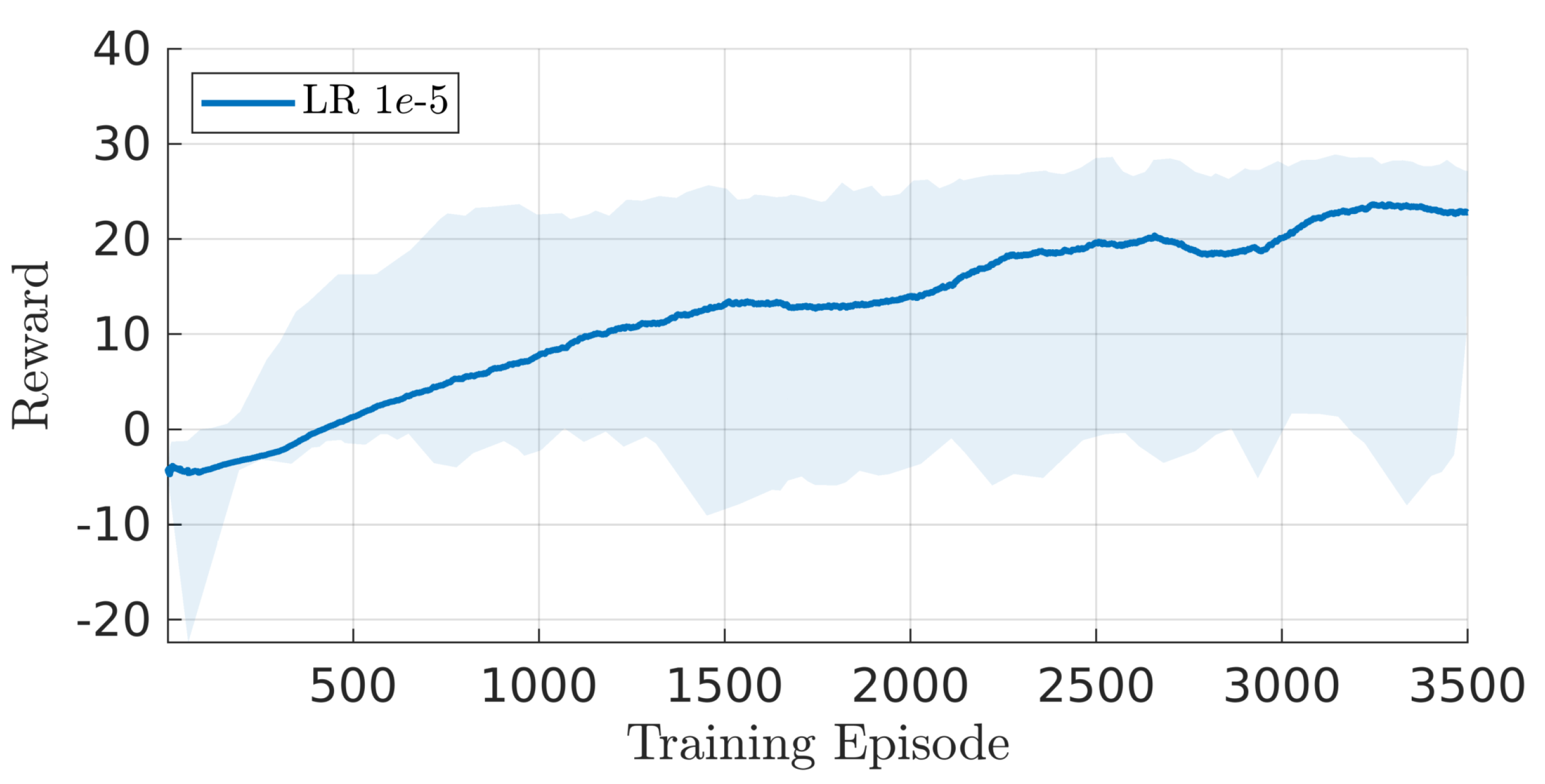
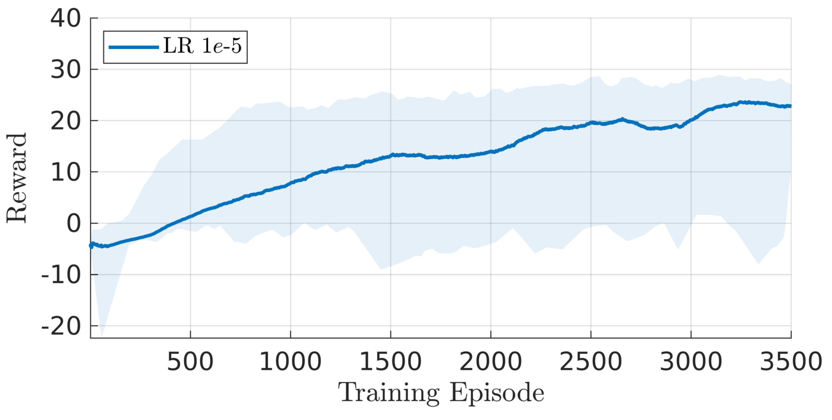
, the mini-batch size is 128, and the training epochs are 4. The agent is trained for 3500 episodes, each of 420 s duration, for a total of 4.9 M timesteps (see Figure 4).

4.1. Agent performance

The agent’s success in a simulation is defined as its ability to keep the end-effector within a selected tolerance from the desired state, in terms of both position and orientation, consecutively for at least

t_{m i n} = 30

s. This differs with respect to what is currently done in the majority of literature, where, once the end-effector enters the selected threshold for the first time, the episode is considered successful and the simulation is terminated. In such a highly dynamic scenario, the latter approach does not prove that the end-effector’s state can remain synchronized with that of the grasping position, and would artificially increase the agent’s performance in the environment.

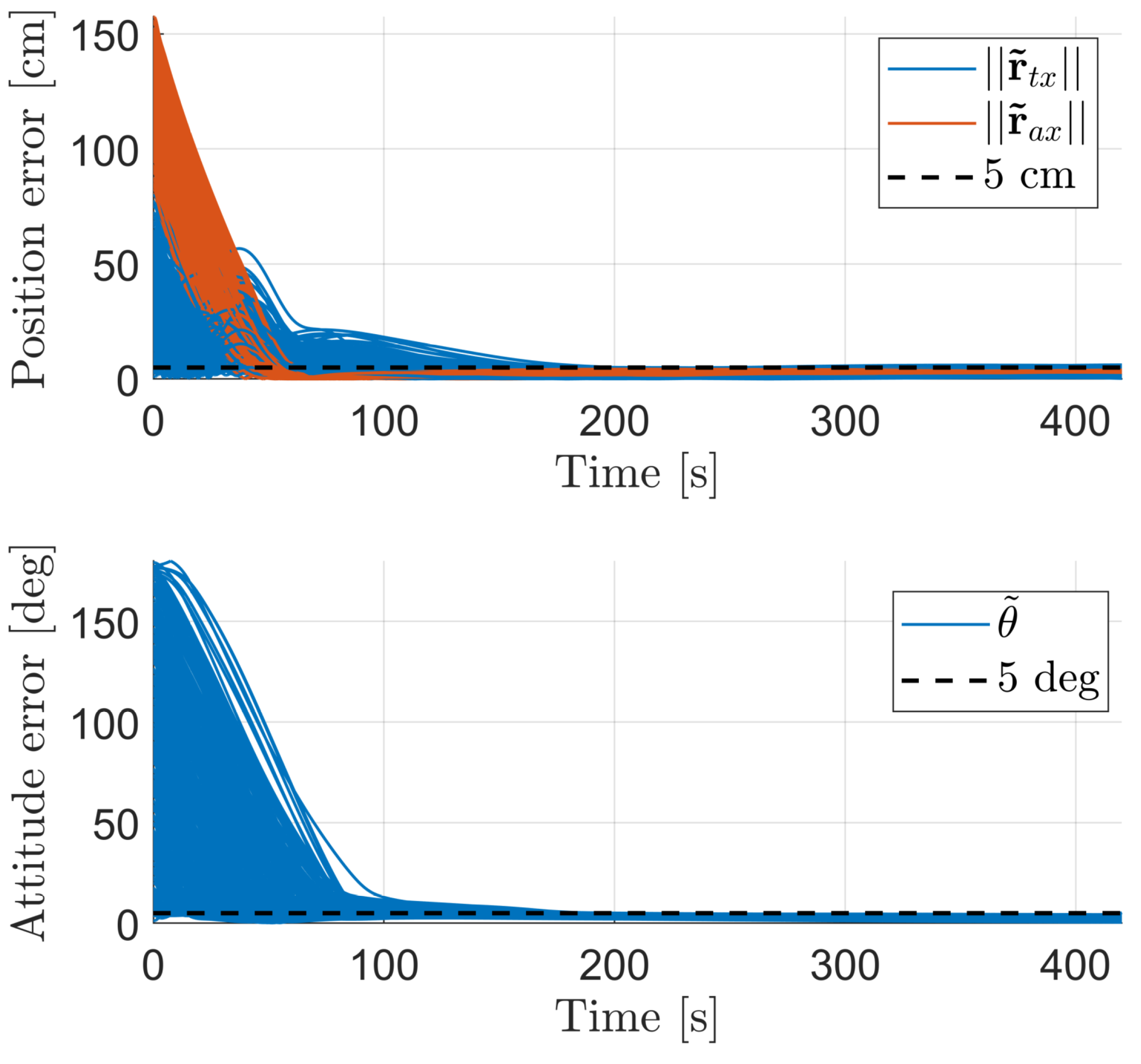
The minimum error thresholds that guarantee a 100% success rate of the agent, and that represent its performance baseline, are

{\tilde{r}}_{a x}, {\tilde{r}}_{t x} < 5

cm and

\tilde{θ} < 5

deg. These results are confirmed through the Montecarlo analysis in Figure 5 and Figure 6, which show that regardless of the grasping point’s location in the target’s body frame, the agent can successfully synchronize the manipulator’s end-effector with the desired state, for consecutive periods that are much higher than

t_{m i n}

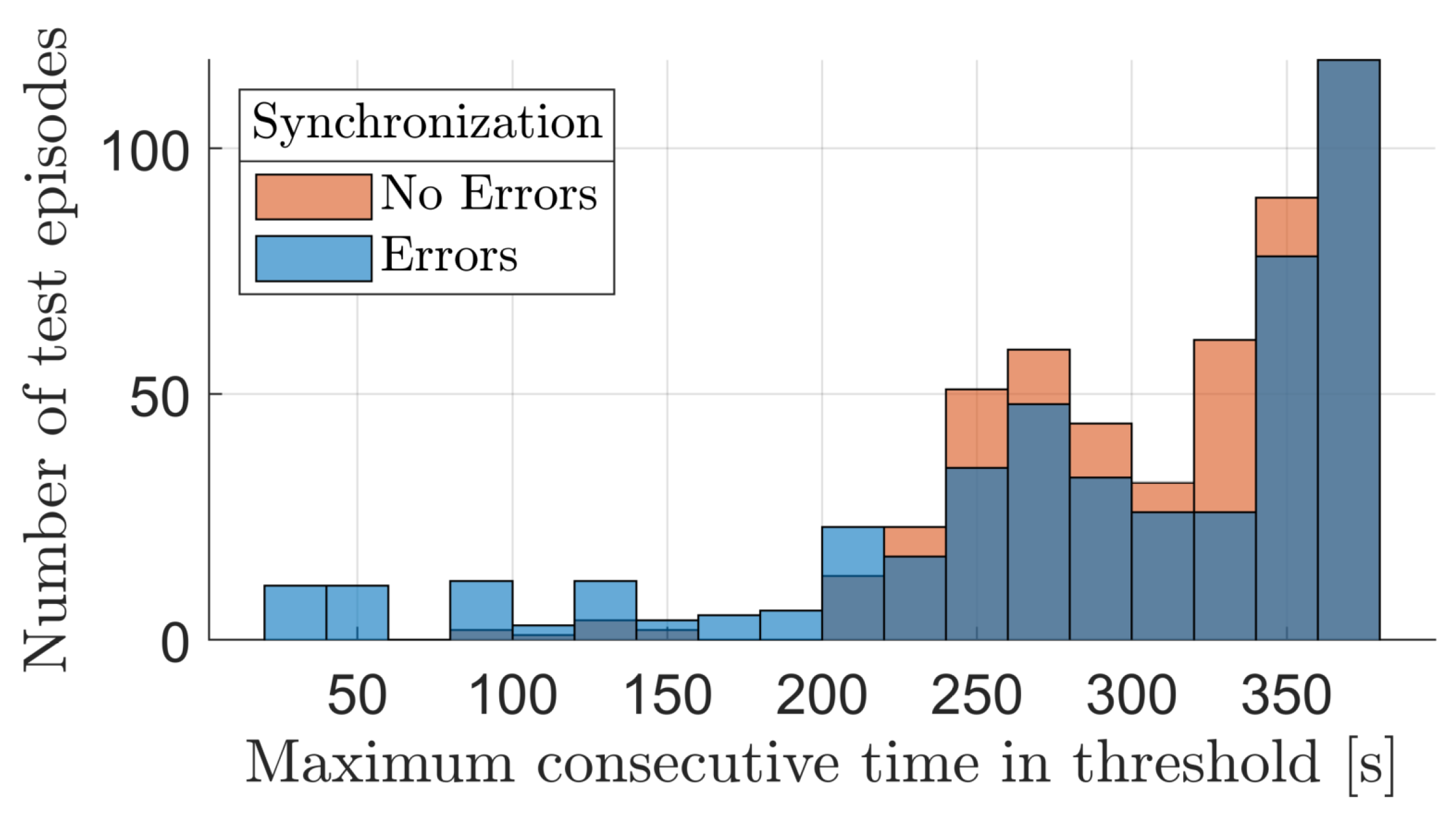
Through a deeper analysis of Figure 6, the average time that the end-effector takes to successfully converge to the desired state is found to be 103 s, and in any case, no episodes take longer than 219 s to accomplish the objective, which is approximately half of the complete episode duration. These values are driven by the randomized initial configuration between manipulator and grasping point, and increase proportionally to the range of motion that needs to be carried out by the robotic arm. Additionally, the average consecutive time that the end-effector stays within the selected error tolerances is 312 s, corresponding to 74% of the total episode duration. This confirms that once the end-effector converges to the desired state, it does not manifest a largely oscillatory behavior.

Building on the few studies found in the literature, this work demonstrates that the proposed AI based robotic arm guidance strategy, when applied to a 7-DoF redundant manipulator which has a randomized positioning and attitude alignment goal for extended periods of time, reliably provides performance in the order of centimeters and degrees. These results show an improvement of what is currently found in literature: in [17] the guidance of a 7-DoF manipulator is trained to achieve an end-effector positioning goal, whereas its attitude is neglected; in [7], a 7-DoF manipulator is trained to accomplish both a positioning and attitude alignment objective, but only the first 6 of 7 joints are controlled, since the end-effector is symmetrical around the last joint’s rotation axis.

4.2. Agent Robustness

The need for highly reactive, adaptive, and autonomous systems anticipated for future close-proximity operations, has been one of the driving factors towards the introduction of AI based methods into spacecraft GNC. Despite being new, the recent applications of DRL in the space field have emerged as promising strategies towards the generation of highly adaptive agents, that can handle unforeseen conditions that have not strictly been trained on, with significant increases towards mission robustness. These capabilities have been shown to be intrinsic to the use of deep neural networks, and if achieved, would provide many benefits supporting the addition of AI into classic GNC systems. To give some preliminary insight into why using such approaches could be advantageous, the agent’s limits and generalization capabilities are stressed in two scenarios that it has not been trained to handle.

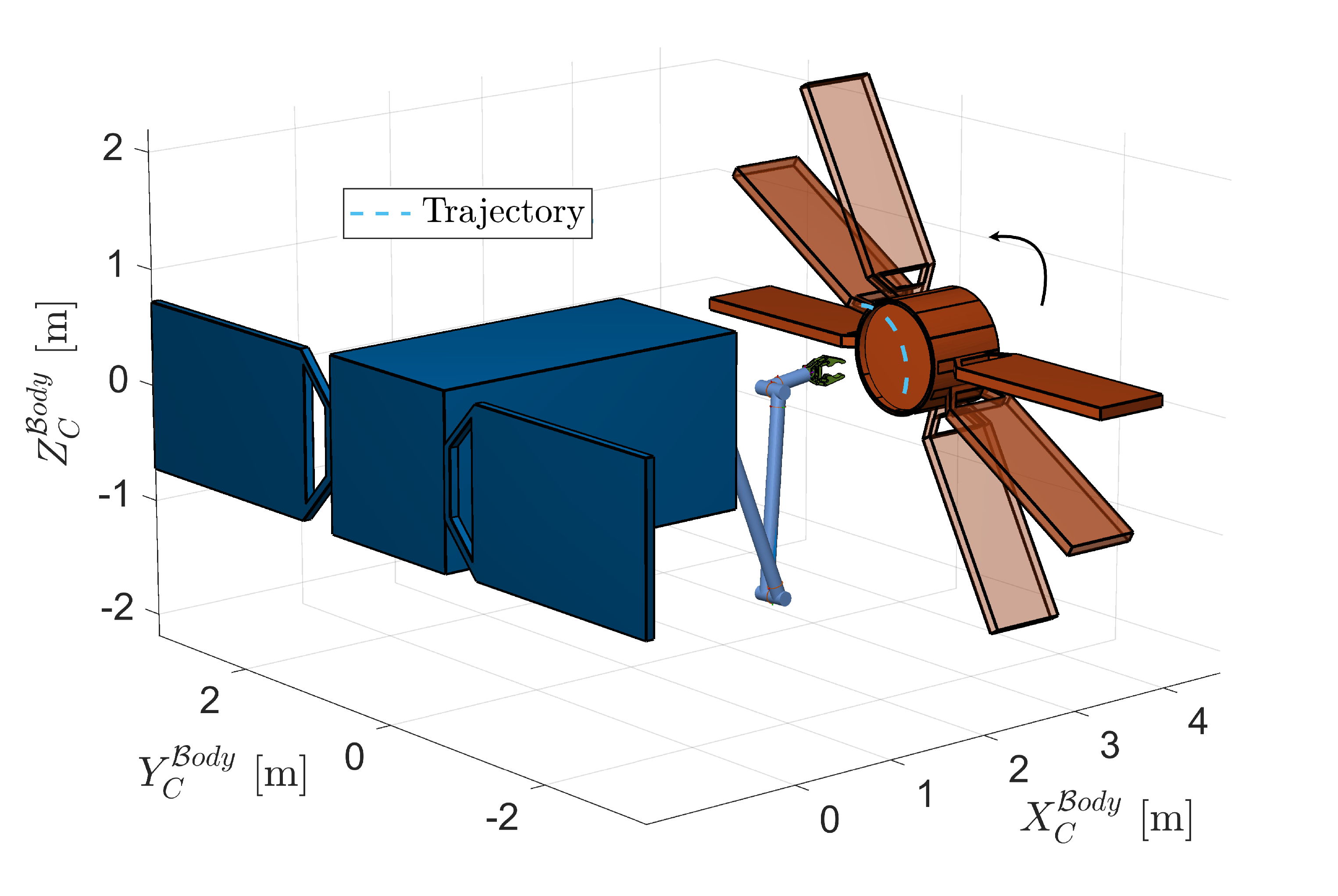
To this extent, errors in the spin rate synchronization around the target’s rotation axis are added, to see whether the agent can adapt to this new scenario without further training. The difference with the previous case, in which the grasping point is static with respect to the SR, is that the end-effector now needs to track a moving point and synchronize its motion with it, maintaining a constant attitude. The maximum spin rate error between the base of the SR and the target is taken from the COMRADE study [18], where the requirement for the angular rate control error is set to

| | ω_{0} - ω_{T} | | < 0.5

deg/s. Hence, the SR’s angular velocity is perturbed each episode by a random value

ω_{e r r} \in [- 0.5, 0.5]

deg/s, as in Equation 16. An overview of this new scenario is provided in Figure 7.

ω_{0} = {[ω_{T} \cdot {\hat{L}}_{T} + ω_{e r r}, 0, 0]}^{⊤}

(16)

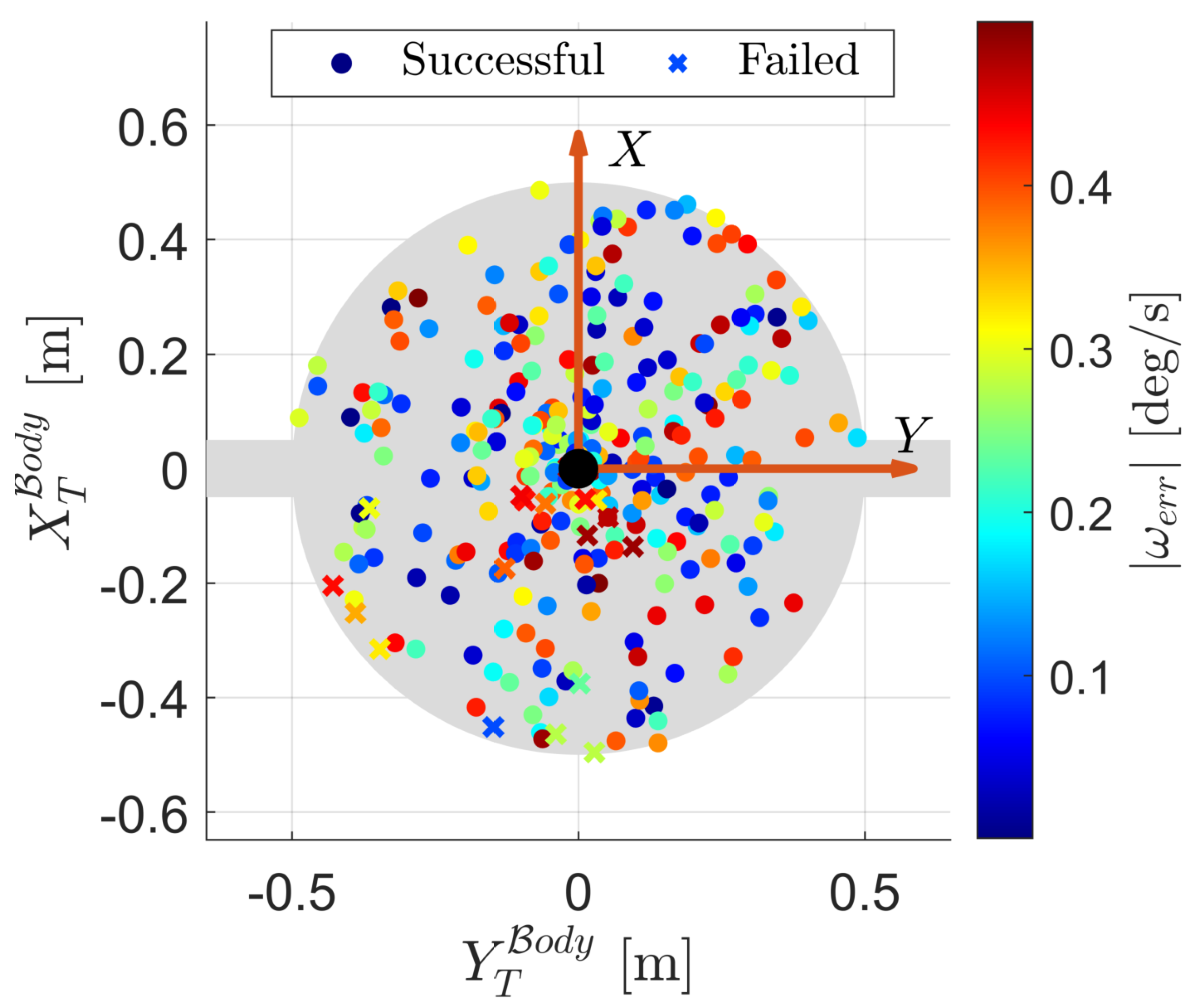
A Monte Carlo analysis is conducted to evaluate the agent’s performance over 500 testing episodes. In these conditions that the agent has never experienced during training, the success rate, defined in the same way as in the previous section, drops to

94 %

. These results show that despite a small decrease in performance, the agent is robust to errors in the attitude synchronization, and is capable of tracking a moving position in time. Referring to Figure 8, it can be seen that the episode failures do not show a correlation to

ω_{e r r}

, since many episodes are successful even when the synchronization error between the SR and target is high in magnitude. Instead, the failures of the agent are more so tied to the initial configuration between the manipulator and grasping point, and are located primarily in the third quadrant.

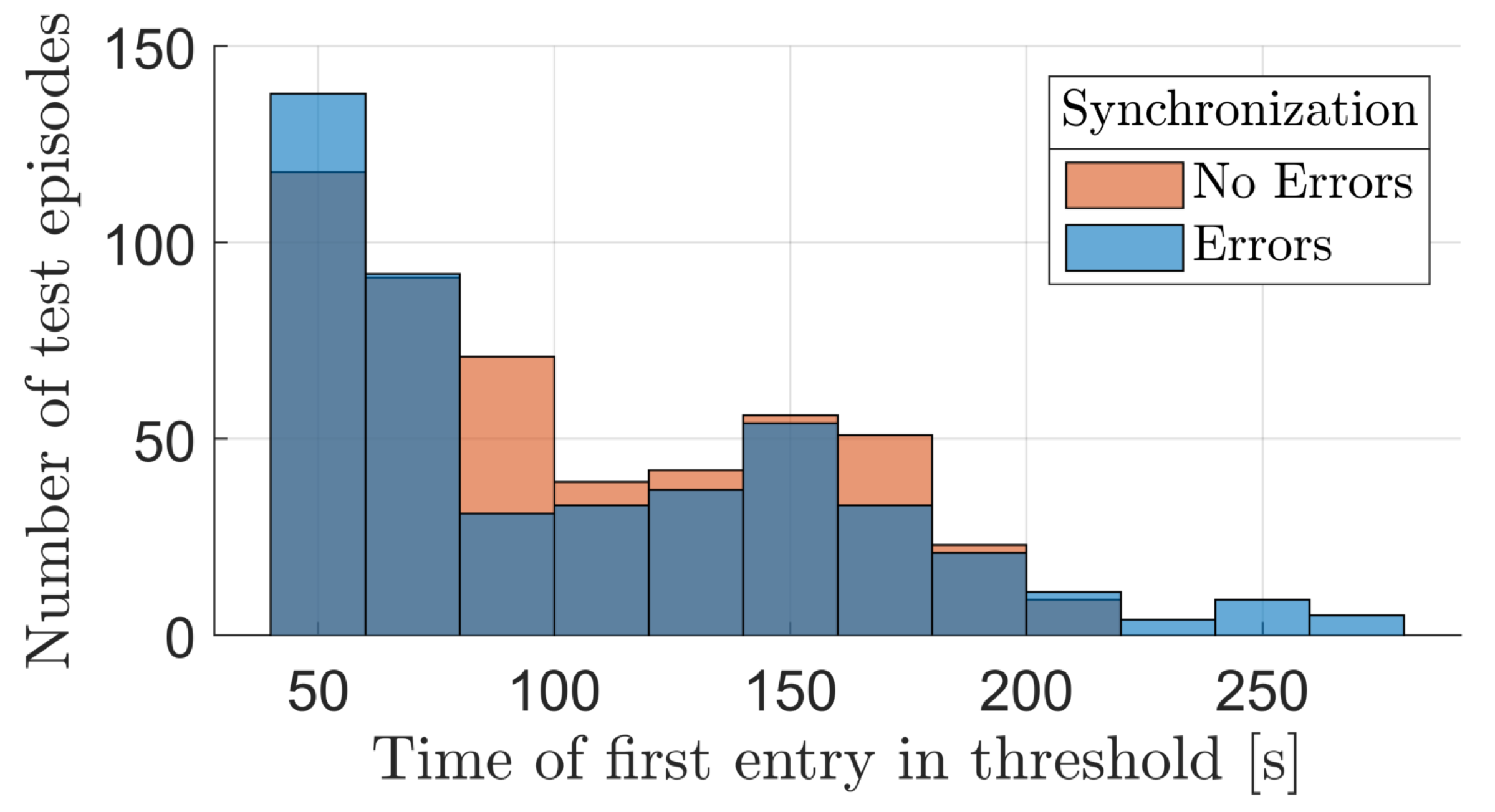
For a more thorough comparison of the agent’s behavior with and without errors in the SR’s base attitude synchronization, the distribution of two performance indicators is reported in Figure 9 and Figure 10: the first figure shows how the time of the end-effector’s first successful entry in the thresholds is distributed among episodes, whereas the second figure shows the distribution of the maximum consecutive time that the end-effector remains inside of the threshold, in each episode. Overall, even when the agent is subjected to a new environment that has not been trained on, its behavior is quite similar to the one it demonstrates in nominal conditions. The main difference is found in terms of outliers in the distributions, which recur more often when synchronization errors are present. Despite this similarity in results, better and more robust performance could be obtained by directly training the agent to handle the more complex environment, where possible.

To better understand how and why the episodes are failing, a sensitivity analysis on the definition of episode success is carried out. The end-effector’s error thresholds

{\tilde{r}}_{a x}, {\tilde{r}}_{t x} < 5

cm and

\tilde{θ} < 5

deg, that need to be guaranteed consecutively for at least

t_{m i n} = 30

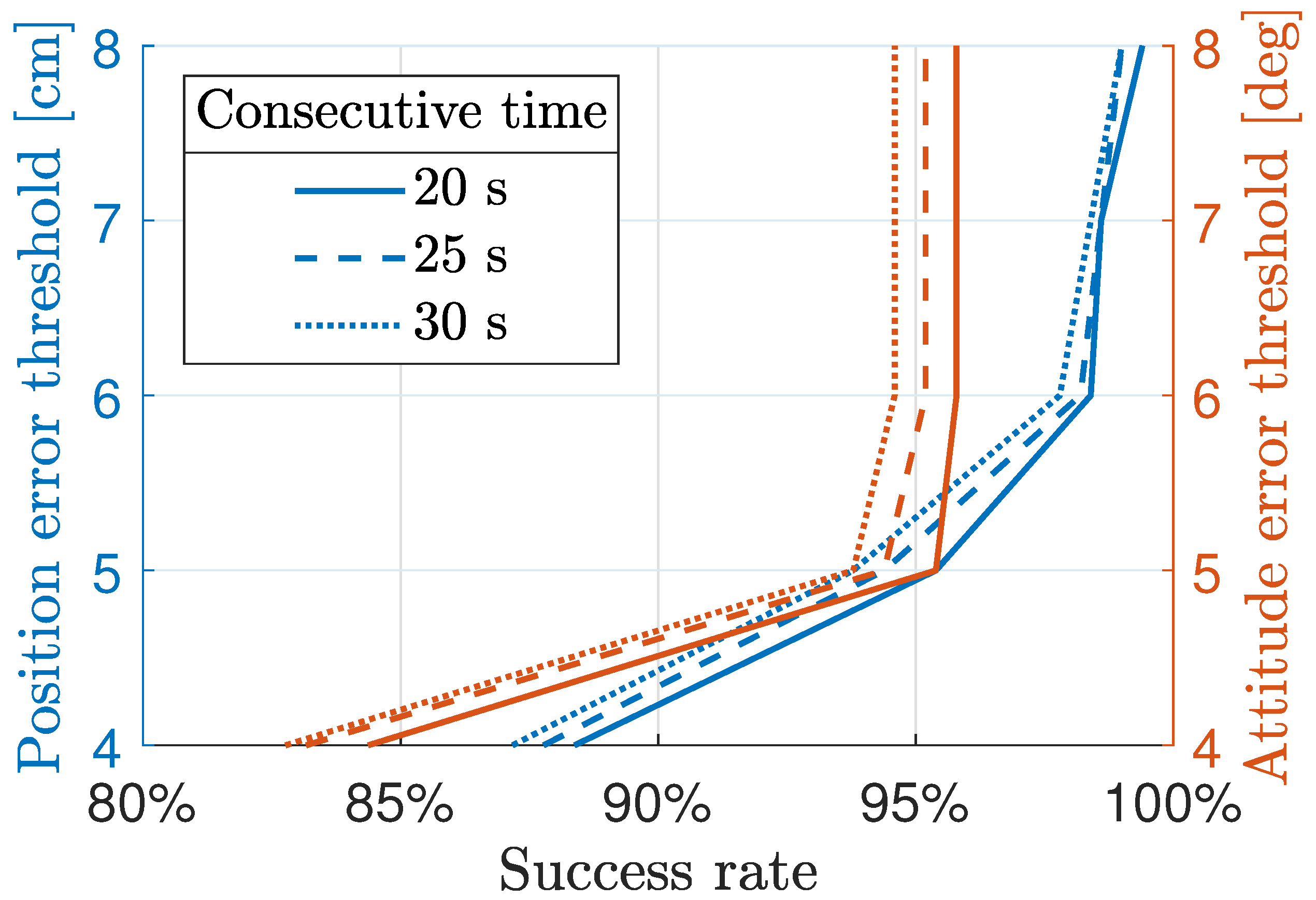
s, have been selected arbitrarily and in real scenarios would be heavily mission-dependent. Figure 11 shows the variation of the success rate over 500 episodes, when these values are changed, in two distinct cases.

The curves associated to the left axis show how the success rate varies in function of the thresholds on ${\tilde{r}}_{a x}$ , ${\tilde{r}}_{t x}$ , and $t_{m i n}$ , while keeping the one on $\tilde{θ}$ fixed.
The curves associated to the right axis show how the success rate varies in function of the thresholds on $\tilde{θ}$ and $t_{m i n}$ , while keeping the ones on ${\tilde{r}}_{a x}$ and ${\tilde{r}}_{t x}$ fixed.

From Figure 11, it can be seen that in both analyses, varying

t_{m i n}

has negligible effects on the success rate, which is explained by the fact that in the majority of cases, the agent can keep the end-effector’s errors low for consecutive periods much longer than

t_{m i n}

. By increasing the threshold on

\tilde{θ}

from its baseline value of 5 deg, the success rate remains unchanged, signifying that the end-effector’s attitude is not the main factor limiting performance. Differently, by increasing the end-effector’s positioning thresholds, the success rate starts to increase, making this value act as the main bottleneck in the obtained performance.

These results are determined by a combination of different effects: firstly, the simple PD controller that is used to control the system after feedback linearization cannot guarantee null steady-state errors, which is a first factor impacting the convergence of the end-effector towards its final desired state; secondly, the agent’s sample time of 0.3 s, coupled with the integration of the actor’s outputs, may also be reducing the agent’s maximum performance, especially once the end-effector errors have been reduced below the baseline threshold values.

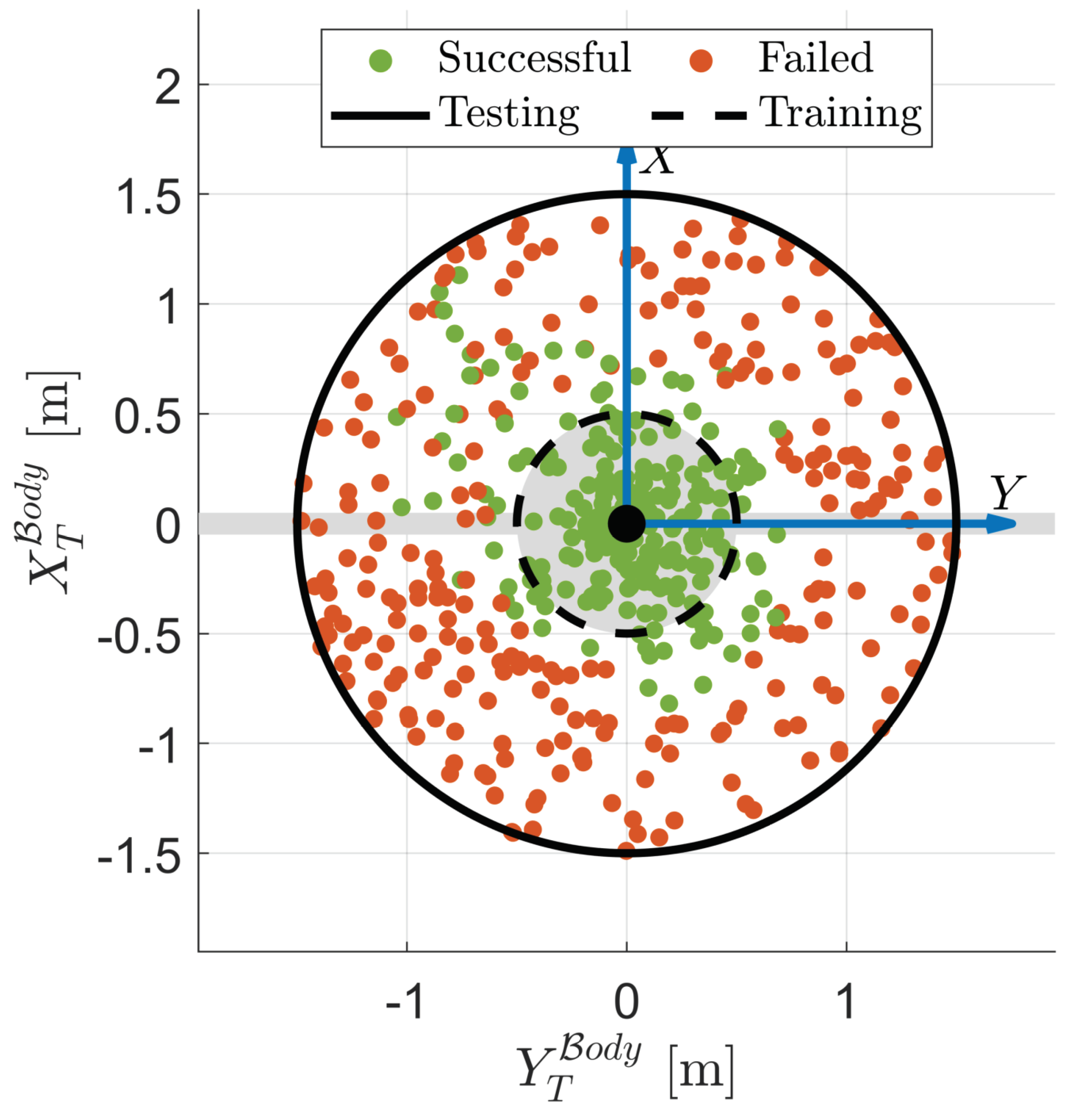
A final test is conducted to further stress the agent’s generalization capabilities, when applied to a Target that is larger than the one used during training. Specifically, the agent has been trained to correctly position and align the end-effector in front of a Target of 50 cm radius, and is instead asked to complete the same randomized objective, but on a Target of 150 cm radius. The agent’s performance is evaluated over 500 testing episodes, and its success rate is shown in Figure 12.

The results show that as the goal position of the end-effector moves outside of the area where it has been trained, the performance drops significantly. Despite this, it has been found that no episodes fail below a radius of 64.5 cm, which shows that the agent can adapt to a condition that it has not experienced during training, and achieve the objective on a Target that is at most 28% larger than the one used in training. To confirm these results in a statistical sense, 200 additional testing episodes are conducted, randomizing the goal position within a radius of 64.5 cm from the center of the Target, and the success rate of the agent remains at 100%.

5. Conclusions

This work proposes a novel autonomous guidance algorithm for the manipulator of a free-flying space robot, allowing to automatically synchronize the end-effector with a desired state fixed to the uncooperative target spacecraft, in a hypothetical IOS mission. The problem is formulated as a POMDP, and solved through the state-of-the-art PPO algorithm. A FNN provides the guidance of the manipulator in real-time based on values retrieved through the navigation system, which is not implemented, and its outputs are provided to a model-based feedback linearization controller, which couples the control laws of the base of the servicer and its manipulator. After the training process, the agent successfully reaches a randomized end-effector state objective, in a highly randomized environment, with a 100% success rate, keeping its errors in terms of position and attitude below thresholds of 5 cm and 5 deg for lengthy consecutive periods. Without any further training, the same agent is found to be robust to errors in the attitude synchronization between SR and target, and can also complete the same objective on a target that is at most 28% larger than the one used during training. Future extensions of similar approaches could obtain better results by using more performant control systems, that guarantee null steady-state errors, or by decreasing the sample time of the agent. The latter would have to be tuned based on the frequency of the values provided by the navigation filters.

Despite the literature on this topic being new and with many shortcomings, the results produced in this work convey that DRL should be investigated further, as a prospective solution to a wider set of robotic IOS scenarios.

Author Contributions

Conceptualization, M.DA., L.C. and M.L.; Methodology, M.DA. and L.C.; writing—original draft preparation, M.DA. and L.C.; writing—review and editing, M.DA., L.C., S.S. and M.L.; Visualization, M.DA.; Data curation, M.DA.; Formal analysis, M.DA.; Supervision, S.S. and M.L.; All authors have read and agreed to the published version of the manuscript.

Funding

This research received no external funding.

Data Availability Statement

Data is contained within the article.

Conflicts of Interest

The authors declare no conflicts of interest.

Abbreviations

The following abbreviations are used in this manuscript:

AI	Artificial Intelligence
APF	Artificial Potential Field
CIM	Convective Inertia Matrix
DNN	Deep Neural Network
DoF	Degree of Freedom
DRL	Deep Reinforcement Learning
FNN	Feedforward Neural Network
GIM	Generalized Inertia Matrix
GNC	Guidance, Navigation, and Control
IOS	In-Orbit Servicing
LR	Learning Rate
MDP	Markov Decision Process
ORM	Orbital Robotics Mission
POMDP	Partially Observable Markov Decision Process
PPO	Proximal Policy Optimization
RL	Reinforcement Learning
SR	Space Robot
TRPO	Trust-Region Policy Optimization

References

Brandonisio, A.; Capra, L.; Lavagna, M. Deep reinforcement learning spacecraft guidance with state uncertainty for autonomous shape reconstruction of uncooperative target. Advances in Space Research 2023. [Google Scholar] [CrossRef]
Capra, L.; Brandonisio, A.; Lavagna, M. Network architecture and action space analysis for deep reinforcement learning towards spacecraft autonomous guidance. Advances in Space Research 2023, 71. [Google Scholar] [CrossRef]
Gaudet, B.; Furfaro, R. Integrated and Adaptive Guidance and Control for Endoatmospheric Missiles via Reinforcement Meta-Learning. arXiv:2109.03880, arXiv:2109.03880 2023. [CrossRef]
Gaudet, B.; Linares, R.; Furfaro, R. Deep reinforcement learning for six degree-of-freedom planetary landing. Advances in Space Research 2020, 65, 1723–1741. [Google Scholar] [CrossRef]
Gaudet, B.; Linares, R.; Furfaro, R. Terminal adaptive guidance via reinforcement meta-learning: Applications to autonomous asteroid close-proximity operations. Acta Astronautica 2020, 171, 1–13. [Google Scholar] [CrossRef]
Moghaddam, B.M.; Chhabra, R. On the guidance, navigation and control of in-orbit space robotic missions: A survey and prospective vision, 2021. [CrossRef]
Li, Y.; Li, D.; Zhu, W.; Sun, J.; Zhang, X.; Li, S. Constrained Motion Planning of 7-DOF Space Manipulator via Deep Reinforcement Learning Combined with Artificial Potential Field. Aerospace 2022, 9. [Google Scholar] [CrossRef]
Wang, S.; Zheng, X.; Cao, Y.; Zhang, T. A Multi-Target Trajectory Planning of a 6-DoF Free-Floating Space Robot via Reinforcement Learning. IEEE International Conference on Intelligent Robots and Systems, 2021; 3724–3730. [Google Scholar] [CrossRef]
Yan, C.; Zhang, Q.; Liu, Z.; Wang, X.; Liang, B. Control of Free-floating Space Robots to Capture Targets using Soft Q-learning. IEEE International Conference on Robotics and Biomimetics 2018. [Google Scholar]
Papadopoulos, E.; Aghili, F.; Ma, O.; Lampariello, R. Robotic Manipulation and Capture in Space: A Survey. Frontiers in Robotics and AI 2021, 8. [Google Scholar] [CrossRef] [PubMed]
Romano, M.; Virgili-Llop, J.; Ii, J.V.D. SPART SPAcecraft Robotics Toolkit: an Open-Source Simulator for Spacecraft Robotic Arm Dynamic Modeling And Control. 6th International Conference on Astrodynamics Tools and Techniques 2016. [Google Scholar]
Sutton, R.S.; Barto, A.G. Reinforcement learning: An Introduction; Westchester Publishing Services, 2018; p. 526.
Schulman, J.; Wolski, F.; Dhariwal, P.; Radford, A.; Klimov, O. Proximal Policy Optimization Algorithms (PPO). arXiv:1707.06347, arXiv:1707.06347 2017.
Schulman, J.; Levine, S.; Moritz, P.; Jordan, M.I.; Abbeel, P. Trust Region Policy Optimization. arXiv:1502.05477, arXiv:1502.05477 2015, pp. 1889–1897.
Mnih, V.; Badia, A.P.; Mirza, M.; Graves, A.; Lillicrap, T.P.; Harley, T.; Silver, D.; Kavukcuoglu, K. Asynchronous Methods for Deep Reinforcement Learning. arXiv:1602.01783, 2016; arXiv:1602.01783. [Google Scholar]
Kumar, V.; Hoeller, D.; Sundaralingam, B.; Tremblay, J.; Birchfield, S. Joint Space Control via Deep Reinforcement Learning. arXiv:2011.06332, arXiv:2011.06332 2020.
Wu, Y.H.; Yu, Z.C.; Li, C.Y.; He, M.J.; Hua, B.; Chen, Z.M. Reinforcement learning in dual-arm trajectory planning for a free-floating space robot. Aerospace Science and Technology 2020, 98. [Google Scholar] [CrossRef]
Colmenarejo, P.; Branco, J.; Santos, N.; Serra, P.; Telaar, J.; Strauch, H.; Fruhnert, M.; Giordano, A.M.; Stefano, M.D.; Ott, C.; Reiner, M.; Henry, D.; Jaworski, J.; Papadopoulos, E.; Visentin, G.; Ankersen, F.; Gil-Fernandez, J. Methods and outcomes of the COMRADE project-Design of robust Combined control for robotic spacecraft and manipulator in servicing missions: comparison between between Hinf and nonlinear Lyapunov-based approaches. 69th International Astronautical Congress (IAC) 2018, pp. 1–5.

Figure 1. Orbital Robotics Mission (ORM) phases.

Figure 2. Motion synchronization scenario.

Figure 3. GNC architecture of SR

Figure 4. Average episode reward throughout training.

Figure 5. Correlation of grasping location to episode success.

Figure 6. End-effector error evolution over 500 testing episodes.

Figure 7. Trajectory of desired end-effector position.

Figure 8. Synchronization error correlation to success.

Figure 9. First end-effector entry in threshold.

Figure 10. End-effector consecutive time in threshold.

Figure 11. Success sensitivity to thresholds.

Figure 12. Generalization to larger target.

Table 1. PD gains for the space robot base and manipulator.

DoFs	Proportional gain ¹	Derivative gain ¹
Base	0.4	0.3
Manipulator	2.5	1.25

¹ PD gains are the same for all base DoFs and all manipulator DoFs, respectively.

Table 2. Actor and Critic Networks hyperparameters.

Layers	Actor neurons	Critic neurons
Input	32	32
1^st hidden	300	300
2^nd hidden	300	300
3^rd hidden	300	300
Output	14	1
Learning Rate	1e-5	1e-5
Activation	$t a n h$	$t a n h$

Disclaimer/Publisher’s Note: The statements, opinions and data contained in all publications are solely those of the individual author(s) and contributor(s) and not of MDPI and/or the editor(s). MDPI and/or the editor(s) disclaim responsibility for any injury to people or property resulting from any ideas, methods, instructions or products referred to in the content.

© 2024 by the authors. Licensee MDPI, Basel, Switzerland. This article is an open access article distributed under the terms and conditions of the Creative Commons Attribution (CC BY) license (http://creativecommons.org/licenses/by/4.0/).

Copyright: This open access article is published under a Creative Commons CC BY 4.0 license, which permit the free download, distribution, and reuse, provided that the author and preprint are cited in any reuse.

MDPI Initiatives

Important Links

Choose an area of interest and we will send you notifications of new preprints at your preferred frequency.

Disclaimer

Redundant Space Manipulator Autonomous Guidance for In-Orbit Servicing via Deep Reinforcement Learning

Abstract

1. Introduction

2. Problem Statement

2.1. Space Manipulator Dynamics

2.2. Target Dynamics

3. Reinforcement Learning Guidance

3.1. Proximal Policy Optimization

3.2. GNC Implementation and Environment

3.3. Action Space and Observation Space

3.4. Reward

4. Training and Results

4.1. Agent performance

4.2. Agent Robustness

5. Conclusions

Author Contributions

Funding

Data Availability Statement

Conflicts of Interest

Abbreviations

References

MDPI Initiatives

Important Links

Subscribe