1. Introduction
Concrete is one of the most crucial and ancient construction materials used in the construction industry (Smarzewski & Stolarski, 2022). The primary raw materials for concrete construction include cement, water, sand, and aggregates. Additionally, certain chemicals or admixtures are incorporated to enhance the initial or final properties of concrete. Globally, around 3 billion tons of raw materials are utilized annually for concrete production (Mehta, 2002; Özturan et al., 2008). However, selecting the appropriate ingredients in the right quantities remains a challenging task for producers aiming to achieve specific concrete strength.
Concrete, being a versatile material adaptable to various requirements and forms, plays a pivotal role in meeting diverse construction needs. Ensuring the desired strength of concrete is critical for safety(Song et al., 2021), as failure to achieve the required strength may result in construction failures, leading to potential loss of life and resources. Traditional strength assessment methods involve complex, time-consuming compression tests under specific laboratory conditions for 28 days (Neville, 2011), and they are susceptible to experimental errors. If concrete fails the test, there is limited scope for adjustments, necessitating a complete restart and prolonged waiting for new results.
Estimating compressive strength before the 28-day mark offers several advantages, including improved efficiency through pre-scheduling of operations. The composition of concrete, its age, water-to-cement ratio, curing conditions, and other factors significantly influence its compressive strength (Ji-Zong et al., 1999). The relationship between concrete strength and its constituents is highly nonlinear, rendering Abrahams’ law insufficient in establishing a dynamic relationship (Özturan et al., 2008).
To address this issue, researchers have explored data-driven models for the evaluation of concrete compressive strength, introducing the concept of machine learning. Machine learning involves training a machine on past data or experiences, enabling it to perform tasks more efficiently than humans. Supervised learning, unsupervised learning, and reinforcement learning are different approaches to machine learning (Jordan & Mitchell, 2015). In supervised learning, the machine learns from labeled data, while unsupervised learning involves unlabeled data. Reinforcement learning occurs when the machine learns from user feedback.
Machine learning models are fed input, which produces output based on applied algorithms(Sarker, 2021). Iterative feedback improves model performance with each repetition. Various algorithms, such as K-Means, Linear Regression, Random Forest, Logistic Regression, Support Vector Machine (SVM), Naive Bayes, K-Nearest Neighbors (KNN), Decision Tree, and Artificial Neural Network (ANN), are commonly used in machine learning. The selection of algorithms depends on data types and result requirements.
This study utilizes ANN, SVM, Regression Tree (RT), and Multiple Linear Regression (MLR) to predict concrete compressive strength using eight attributes: Water, Cement, Coarse Aggregate, Blast Furnace Slag, Age, Superplasticizer, Fly Ash, and Fine Aggregate.
2. Methods
To identify the optimal model for predicting future data, various regression methods were employed in this study. Specifically, four distinct approaches were utilized to establish a model for predicting concrete compressive strength based on several dependent variables such as cement, water, aggregates, and others. The four methods employed in this investigation include Artificial Neural Network, Multiple Regression Analysis, Support Vector Machine, and Regression Analysis.
2.1. Artificial Neural Network(ANN) Model
Artificial Neural Networks (ANNs) are information processing systems based on how biological nervous systems, like the brain, process information (Mr. Dongare Sadanand, Dr. Sachin Bhosale, 2023). An artificial neural network is a network of interconnected nodes, referred to as artificial neurons, designed to emulate the functioning of the human brain (Chou & Tsai, 2012; Kaveh, 2002). These neurons are linked to each other, facilitating the transmission of signals from one to another. Upon receiving a signal, each neuron processes it and generates an output computed by a non-linear function of the sum of its inputs. Neurons possess weights that dynamically adjust during the learning process to enhance performance. The network comprises different layers, with each layer containing varying numbers of neurons, ranging from tens of thousands to less than ten (Zupan, 1994).
The distinctive feature of artificial neural networks, setting them apart from conventional problem-solving methods, lies in their learning capability. The learning process, termed training, allows the network to adapt its problem-solving approach based on the nature of the problem and specific requirements. However, this adaptability also introduces a challenge, as the network’s results can sometimes be unpredictable due to its unique problem-solving approach (Maind & Wankar, 2014).
For processing with an artificial neural network, available data is initially randomly divided into three sets. The first set is the training set (60 to 75%), followed by the validation (or fine-tuning set, 15 to 20%), and the test set (15 to 20%). These sets are utilized in the training, validation, and testing steps, respectively. Each step serves a specific purpose in the artificial neural network workflow. Training aims to minimize errors, such as mean square error (MSE) or root mean square error (RMSE), by adjusting the connections between neurons and weights to produce output results as close as possible to the target values. Validation steps operate independently from the training set, contributing to the refinement of the model. Finally, the testing process assesses the accuracy of the developed model (F & K, 2016).
2.2. Multiple Linear Regression Model
A regression model illustrates the relationship between a dependent variable, denoted as y, and an independent variable, denoted as x. When there is only one independent variable, it is referred to as a simple regression model. However, when there are multiple independent variables, the model is termed a multiple regression model. Regression models serve to identify correlations between predictors and criterion variables, aiming to uncover relationships between them(Yan & Wang, 2022).
In a simple regression model, the objective is to find the best-fit line that accommodates all the data for the dependent and independent variables. Conversely, a multiple regression model seeks a plane that optimally fits all available data. Models with more than two independent variables introduce complexity, yet they can still be analyzed using various methods. In interactions, the relationship between an independent variable and the dependent variable may be linear, curvilinear, or dependent on the value of another independent variable (Aiken et al., 2012). Equation 1 outlines the fundamental structure of a multiple linear regression model.
where y represents the output data, 𝑋
𝑘’s are the input variables serving as independent variables, and 𝑎0, 𝑎1, 𝑎2, …, 𝑎𝑛 are the partial regression coefficients. The method of least squares is employed in multiple regression to determine the best-fitting line and regression coefficients (Brown, 2009). Various software tools, such as Mathematica, Stata, and Matlab, offer a matrix approach for solving multiple linear regression problems, as demonstrated in studies by (Araiza-Aguilar et al., 2020; Kohler & Kreuter, 2005).
2.3. Support-Vector Machines (SVMs)
Support Vector Machines (SVMs) is designed to learn from training data and aim to generalize its knowledge to accurately predict outcomes on new, unseen data(Campbell & Ying, 2022). SVMs have emerged as a significant tool in pattern recognition and regression, known for their excellent generalization performance (Shevade et al., 2000). This method is often considered a formidable competitor to Artificial Neural Network (ANN) models, capturing the attention of researchers in both the neural network and programming communities. SVMs find applications in real-world scenarios and were initially introduced by Vapnik and his colleagues (Boser et al., 1992). Capable of addressing both classification and regression problems in supervised machine learning, SVM separates two classes of points using a hyperplane, akin to logistic regression and linear regression.
What sets SVM apart is its unique approach of creating two marginal lines parallel to the hyperplane. These margin lines ensure a certain distance, allowing easy linear separability for both classification points. The parallel margin lines pass through the nearest points from each class to the hyperplane. Therefore, SVM not only focuses on a single hyperplane but creates two parallel hyperplanes. One hyperplane passes through the nearest positive points, and the other passes through the nearest negative points, maximizing the distance between them. This configuration provides the SVM model with a cushion to better divide the two classes, resulting in a more generalized and effective predictive model.
Support vectors are the points that pass through the margin line or plane, which can be one or more. While linearly separable data simplifies the creation of the hyperplane, SVM employs a technique called SVM kernel for non-linearly separable data. The SVM kernel aims to transform 2-D or low-dimensional data into higher dimensions for improved classification by the hyperplane. Various types of kernels are available, such as polynomial, RBF, sigmoid, etc., chosen based on the data and scenario. Among this RBF is the most famous and mainly used for calculation (Ting et al., 2018).
This study employs the MATLAB application for the SVM model, utilizing the regression learner add-ons app under the Machine Learning and Deep Learning section. The process involves importing data, selecting the SVM model, and running the analysis. MATLAB offers different SVM models, including linear, quadratic, cubic, fine Gaussian, medium Gaussian, and coarse Gaussian SVMs. The output is presented in terms of Root Mean Squared Error (RMSE), where the model with the smallest RMSE value indicates better performance and is chosen for further prediction with test data. The simplicity and speed of this entire process make it highly efficient.
2.4. Regression Tree (RT)
A decision tree is a tree-like structure where each node represents a test on a given feature or attribute, and the branches coming out of the node indicate the outcome of the test. The nodes with no branches, also known as decision nodes, are called leaf nodes or terminal nodes, holding the class label, which can be a classification or regression value. The top node in the tree structure is termed the root node.
Decision trees can be used for decision-making purposes, providing a visual and explicit representation of the decision process. They apply to both classification and regression tasks, with regression trees specifically designed for handling continuous data. The root node initially encompasses all the data in the dataset, and based on the test results, the dataset splits, known as a splitting action. The process continues with additional tests on subsequent decision nodes until a class or value is assigned to the leaf node.
Despite their intuitive tree-like structure, decision trees can become complex and lengthy in practice, making interpretation challenging. They also perform feature selection or screening of variables and accommodate both categorical and numerical data. Two types of decision trees exist in machine learning algorithms: Regression trees, used for continuous outcomes, and classification trees, employed when the outcome falls into a finite number of groups. Together, they are referred to as Classification and Regression Trees (CART). In regression trees, each leaf represents a numeric value, while classification trees yield results like true or false or other distinct categories in their leaves.
Regression trees commonly use impurity measures such as least squares and least absolute deviation (Moisen, 2008). They are adept at handling intricate data structures. This study utilizes MATLAB software for processing regression trees through regression learner add-ons. The software tests three different regression tree models: fine, medium, and coarse tree models. It evaluates each tree’s performance in terms of Root Mean Squared Error (RMSE). The regression tree model with the lowest RMSE is selected for further processing and prediction, making the overall process straightforward and efficient.
2.5. Data Description
In pursuit of the objectives outlined in this study, a dataset consisting of 1030 entries, each containing various parameters related to concrete mix, along with their corresponding compressive strengths, was sourced from the online platform Kaggle. Prior to analysis, the collected data underwent a meticulous accuracy check and subsequently underwent a process of data preprocessing using MATLAB software. This initial phase ensures the quality and readiness of the dataset for further analysis and investigation.
2.5.1. Data Preprocessing
Raw data obtained from any source may not be directly suitable for data analysis without undergoing necessary preprocessing steps. This is because the data may contain missing values, erroneous inputs, or formats that are not conducive to analysis. These issues could introduce abnormalities in the output, necessitating careful preprocessing to make the data suitable for use.
In this study, various data preprocessing steps were employed. These included checking for outliers, handling null values, and feature scaling. These operations not only render the data usable but also contribute to increased accuracy of the results.
Table 1 presents different statistics related to the parameters utilized in this study, offering insights into the characteristics of the dataset after undergoing the specified preprocessing steps.
2.5.2. Association of Data
a) Variance
Variance represents how much data is spread in the dataset. It calculates how far each number is present in the dataset from the mean of the whole data. It is an important way to find out the random variable that can be present in the given range. It is calculated by squaring the difference between mean and each variable and adding them together then dividing the sum with the total number of variables. The calculating formula for finding the variance is: The variance is a statistical measure that quantifies the degree to which data points in a dataset deviate from the mean. It assesses the spread or dispersion of the data. Specifically, variance calculates how far each individual data point is from the mean of the entire dataset. The calculation involves squaring the difference between each data point and the mean, summing these squared differences, and then dividing by the total number of data points.
Mathematically, the formula for calculating the variance (
) is as follows:
‘X’ represents individual data points from the dataset, while ‘μ’ denotes the mean value calculated across all datasets. ‘N’ stands for the total number of data points in the dataset. A higher variance value suggests that the data points in the dataset are more dispersed from the mean, indicating greater variability. Conversely, a lower variance value suggests that the data points are closer to the mean, indicating less variability.
Table 2 presents the variance values for various attributes considered in this study.
b) Correlation
The correlation coefficient for any pair of attributes within a dataset always falls within the range of -1 to +1. This metric is utilized to gauge the degree of relationship between a given attribute and others present in the dataset.
A negative correlation coefficient indicates that as the value of one attribute increases, the value of the other decreases. Conversely, a positive correlation coefficient suggests that an increase in the value of one attribute corresponds to an increase in the value of the other. When the correlation coefficient is close to +1, it indicates a stronger correlation between the two attributes. For identical attributes, the correlation coefficient is exactly 1, signifying identical behavior.
Table 3 displays the correlation coefficients between compressive strength and other attributes or variables. A higher correlation coefficient between cement and compressive strength implies a significant role of cement in achieving higher strength. This pattern holds true for various other variables as well.
2.6. Evaluation of Findings
Four distinct methods were employed to assess the generalization efficiency of the trained model, aiding in the identification of models with superior performance and accuracy. The first method utilized in this study is the Mean Absolute Deviation (MAD). MAD is calculated by dividing the sum of the absolute differences between the actual and predicted values by the total number of observations. This metric provides insights into the variability within a dataset. A lower MAD value indicates better model performance. The equation for MAD calculation is as follows:
In this study the unit of MAD will be MPa. The second method is coefficient of correlation (CC). The formula to calculate the CC is
The value of CC should be approaching 1. Which will represent the best model.
Another method is Root Mean Square Error (RMSE) which is the standard deviation of residuals. In other words, it tells how concentrated the data is around the line of best fit.
The lower value of RMSE is indicative of good performance. In this study the unit of RMSE will be MPa.
And the last method is known by the name of Mean Absolute Percentage Error (MAPE). It is also a statistical measure of how accurate a forecast system is. It measures accuracy in percentage. It is calculated by the formula
Lower MAPE values show more accuracy of the given method. In all the above four equations, A
t is the actual value while F
t is the predicted value of our trained model and n is the size of the dataset.
3. Results and Discussion
3.1. Artificial Neural Network
In this study on artificial neural network models, eight different input variables were utilized to predict concrete compressive strength using the ANN. A total of 1030 specimens were randomly divided into 70% for training and the remaining 30% equally divided for validation and testing. Various training algorithms were employed to optimize results, including different network types such as Feed Forward Back Prop, Cascade-forward backprop, Competitive, Elman backprop, Feed-forward distributed time delay, Feed-forward time delay, NARX, NARX Series-parallel, Layer Recurrent, and others.
Throughout the process, the input data and target data remained constant. There was flexibility in selecting different training functions, such as TRAINLM, TRAINOSS, TRAINR, TRAINRP, and many others. Additionally, two distinct Adaption learning functions, LEARNGD and LEARNGDM, were considered for improved results. Three performance functions, namely MSE, MSEREG, and SSE, were employed for evaluation.
Crucial factors influencing the ANN model’s performance include the number of neurons and the number of hidden layers. The transfer functions of each layer, such as TANSIG, PURELIN, and LOGSIG, were also tested to assess model performance.
Table 4 presents various architectural models used in the process, where, for example, ‘8-10-1’ denotes 8 input variables, 10 neurons, and 1 output. Similar notations apply to other architectures, with the first and last numbers representing input and output, respectively, and the numbers in between indicating neurons in the hidden layers.
Table 5 outlines the optimum parameters for the best-trained model, providing valuable insights into the configuration that yielded the highest performance.”
Here 8-15-1 model is selected as the best ANN model as this model gives the higher accuracy.
Figure 1 illustrates the architecture of the best-trained model, featuring two hidden layers. The first hidden layer consists of 15 neurons, while the second hidden layer employs 10 neurons. TANSIG transfer function is applied to each hidden layer.
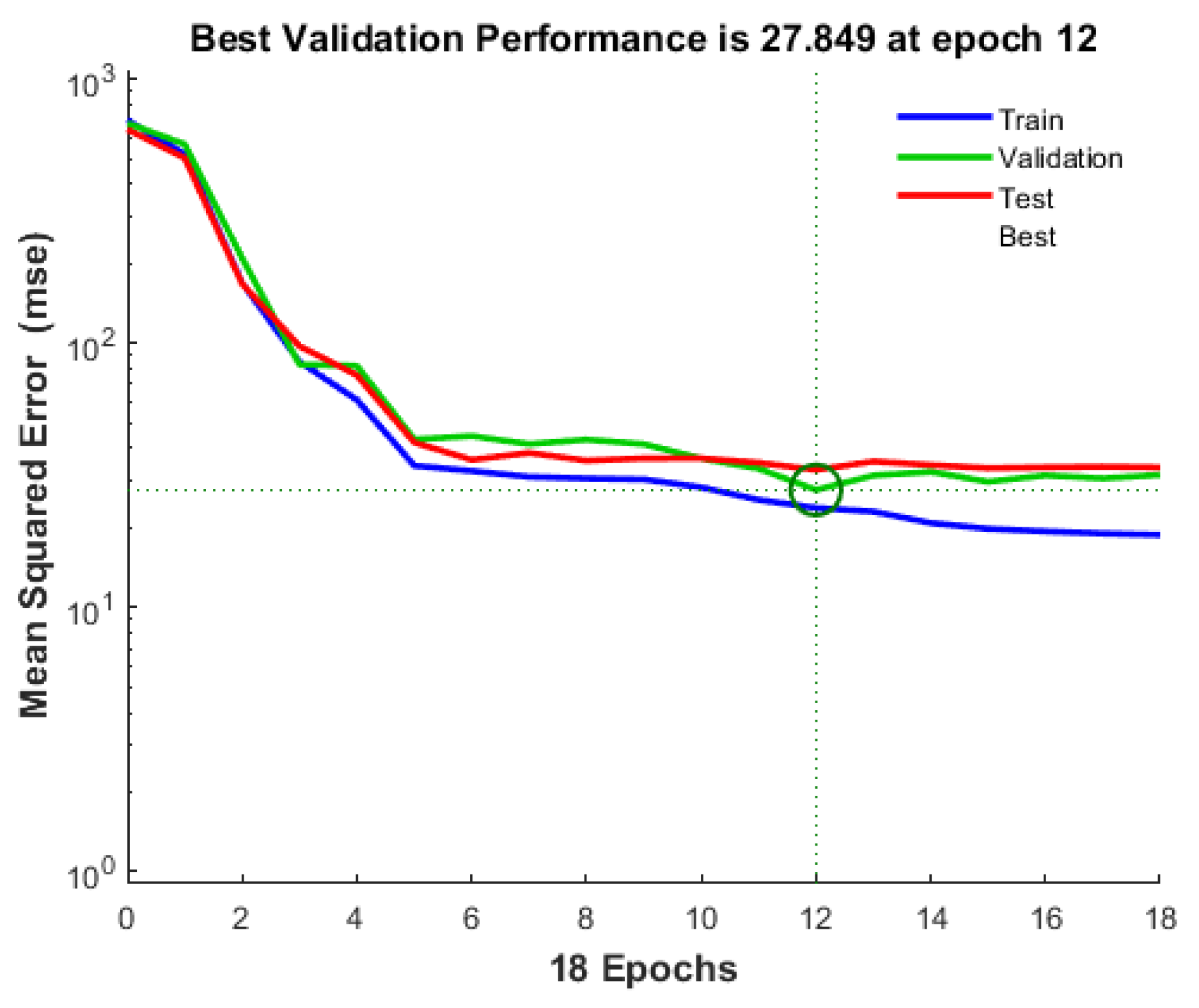
Figure 2 displays the validation performance throughout the training, validation, and testing steps. This visualization presents the Mean Square Error (MSE) for the best-performing architecture, indicating the network’s learning progress. Notably, at epoch 12, the model achieved its optimal validation performance with the lowest mean square error. This observation suggests that the model continued training until the network error on the validation vectors reached its minimum value. The evaluation process concluded after 6 additional iterations, stopping at epoch 18, immediately following the epoch 12 with the best validation performance.
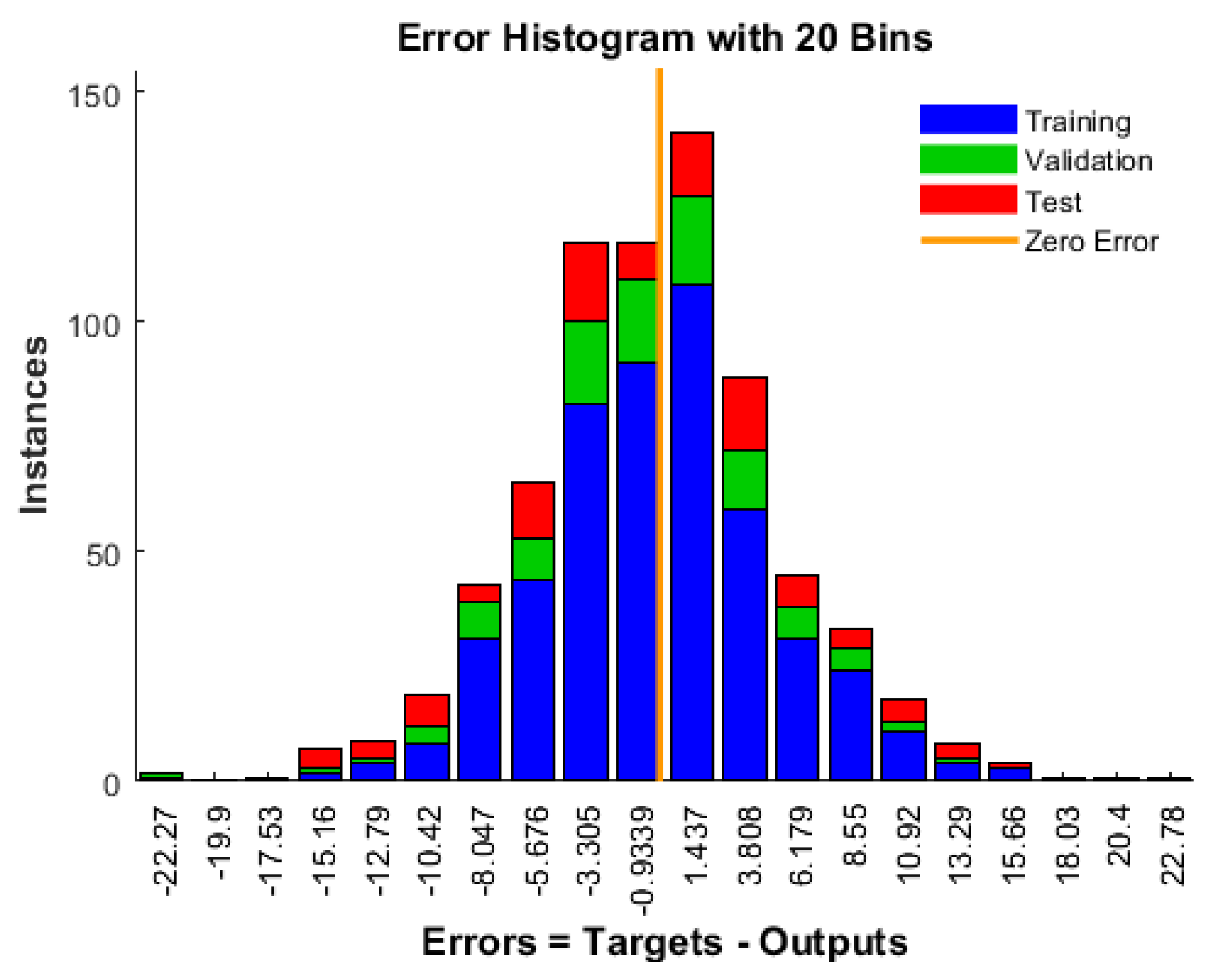
Figure 3 depicts the error histogram of the best-trained model, wherein the error range is segmented into 20 smaller bins. Bins are represented by the number of vertical bars on the graph. The error range on the graph spans from negative 22.27 to positive 22.78. In the graph, the blue bars denote values for training, the green bars represent validation, and the red bars signify test values. The zero error line is also featured on the graph. A higher concentration of bin heights near the zero error line indicates a well-performing model. In this context, error is calculated as the difference between predicted compressive strength and measured compressive strength.
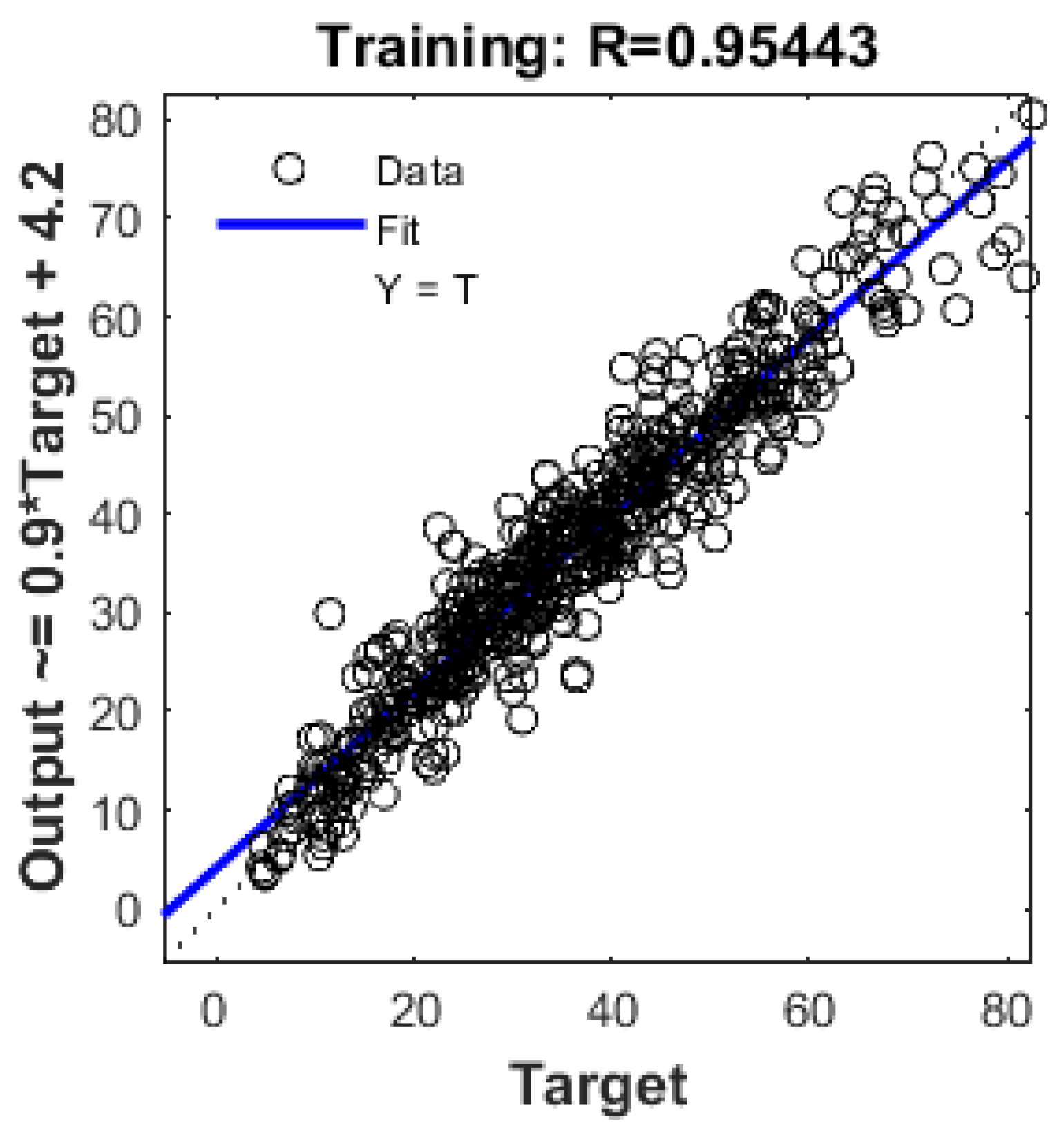
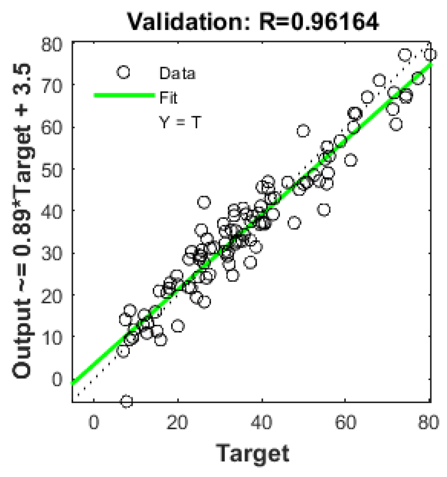
Figure 4 and
Figure 5 illustrate the relationship between predicted compressive strength and measured compressive strength. In
Figure 5, which represents the training steps, the value of R is 0.95443, indicating a favorable result for the model. The same positive representation holds for
Figure 6, which showcases the results for validation steps, with an R value of 0.96164.
3.2. Multiple Linear Regression
This study employed a total of 1030 specimen samples for training and testing the multiple linear regression model. Each specimen sample consists of 8 different input variables representing various attributes of concrete manufacturing. The output variable provides the compressive strength of concrete. For model training, 721 samples (70% of the total) were selected, while the remaining 309 samples (30% of the total) were designated for testing the model’s performance.
During the training step, the weight parameters for different attributes were determined as follows: 0.1194, 0.1074, 0.089, -0.1909, 0.1989, 0.0162, 0.0145, and 0.1229, respectively, for the 8 different attributes. Additionally, the value of α0 was found to be -9.2973.
The multiple linear regression equation is expressed as follows:
Here, A2, B2, C2, etc., represent the values of input variables such as cement content, blast furnace slag, fly ash, water content, superplasticizer, coarse aggregate, fine aggregate, and the number of days (age), respectively.
Table 6 displays the performance measurement of the generated model for the test data.
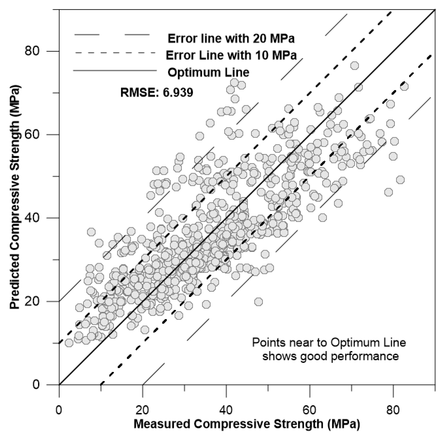
The graph below shows the measured vs. predicted compressive strength with RMSE=6.9395.
The figure above illustrates two different error lines and an optimum line. The optimum line consists of points where the predicted values equal the measured values of concrete strength. The error lines are situated within a range of ±10 MPa and ±20 MPa on both sides of the optimum line. A higher concentration of points near the optimum line indicates a good performance result. When points fall between the optimum line and the first error line (closer to the optimum line), the model is performing well with some error. If some points extend beyond the first error line, the model exhibits a slightly higher error. In this case, a significant number of points are scattered outside the first error line, and even some are outside the second error line. This suggests that the model is not performing well and is lacking in higher accuracy in its predictions.
3.3. Support Vector Machine (SVM)
The Support Vector Machine (SVM) model employed the same sample data to facilitate a proper comparison of different model performances. The entire dataset was randomly divided into 70% for training and 30% for testing. The model training was conducted using the MATLAB Regression Learner application. Various SVM configurations were explored to achieve higher accuracy. The results of the trained model are depicted in
Table 7, where cubic SVM is found to be better among others. This model is exported to the further prediction of future data.
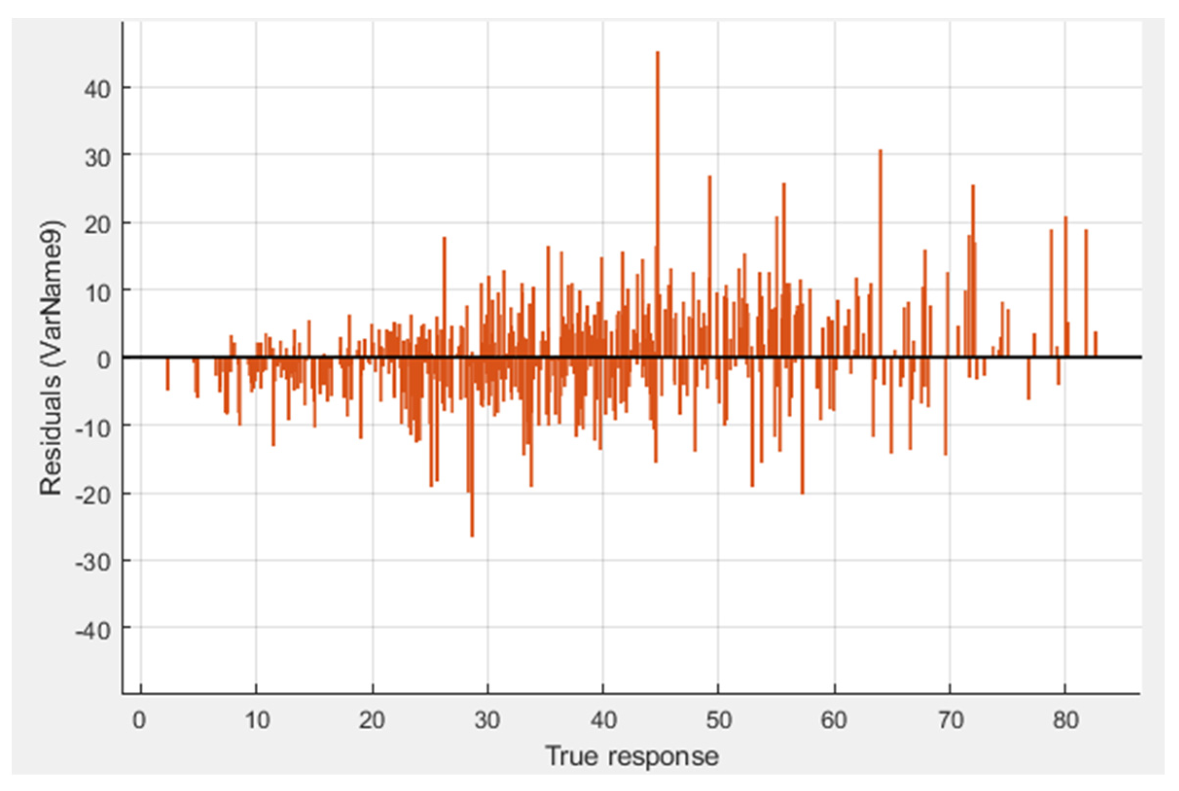
Figure 7 shows the residual graph of the true value and residual value.
3.4. Regression Tree
Similarly to the last two models, the Regression model also utilized the same set of 1030 sample data, with the data division for training and testing purposes. Each sample data point comprises 8 different input variables and 1 output variable. The various input variables represent parameters for concrete manufacturing, including the weight of cement, different types of aggregate, water, and other crucial factors. The model training was carried out using the MATLAB Regression Learner application, with the selection of ALL regression trees to achieve higher accuracy among the available options in MATLAB. The results of the trained model are presented in
Table 8.
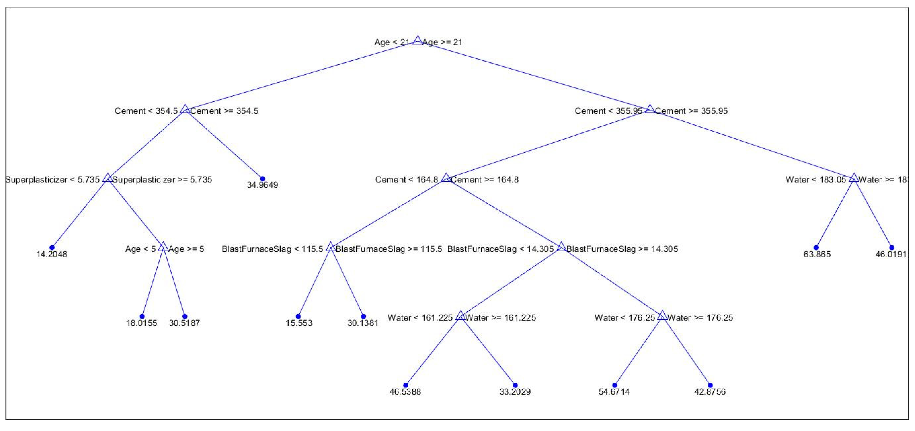
Based on the above results, it is observed that the Fine Tree model outperforms the others. This model has been selected for further predictions on future data, and its decision tree structure is examined for insights.
Figure 8 illustrates the regression tree with a pruning level of 94 out of 106.
3.5. Performance Comparison
Optimum parameters were determined for all the models tested in this study. For the ANN model, various parameters were altered, including the number of hidden layers, the number of neurons, and the training model. Each change in these parameters led to a corresponding change in the model’s results. Multiple attempts were made using trial and error methods to identify the optimum parameters. Similar steps were undertaken for the other models to find the best fit.
Table 9 presents a comparison of the performance measurements for different models.
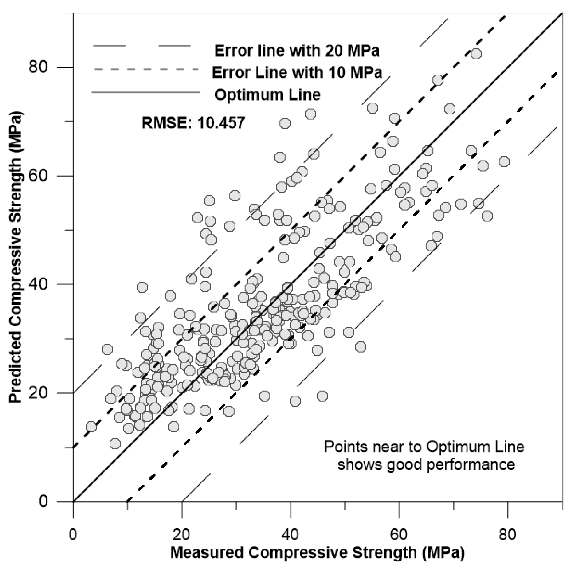
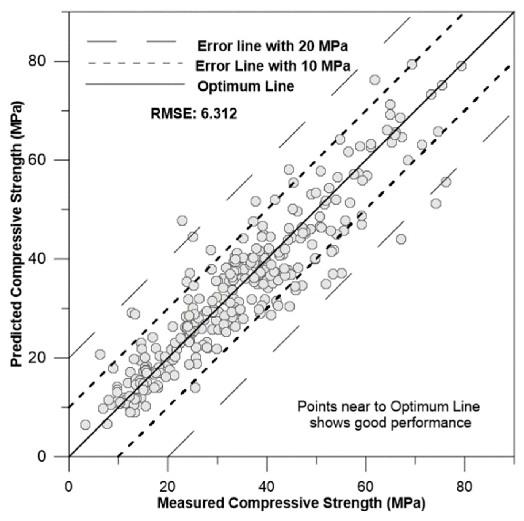
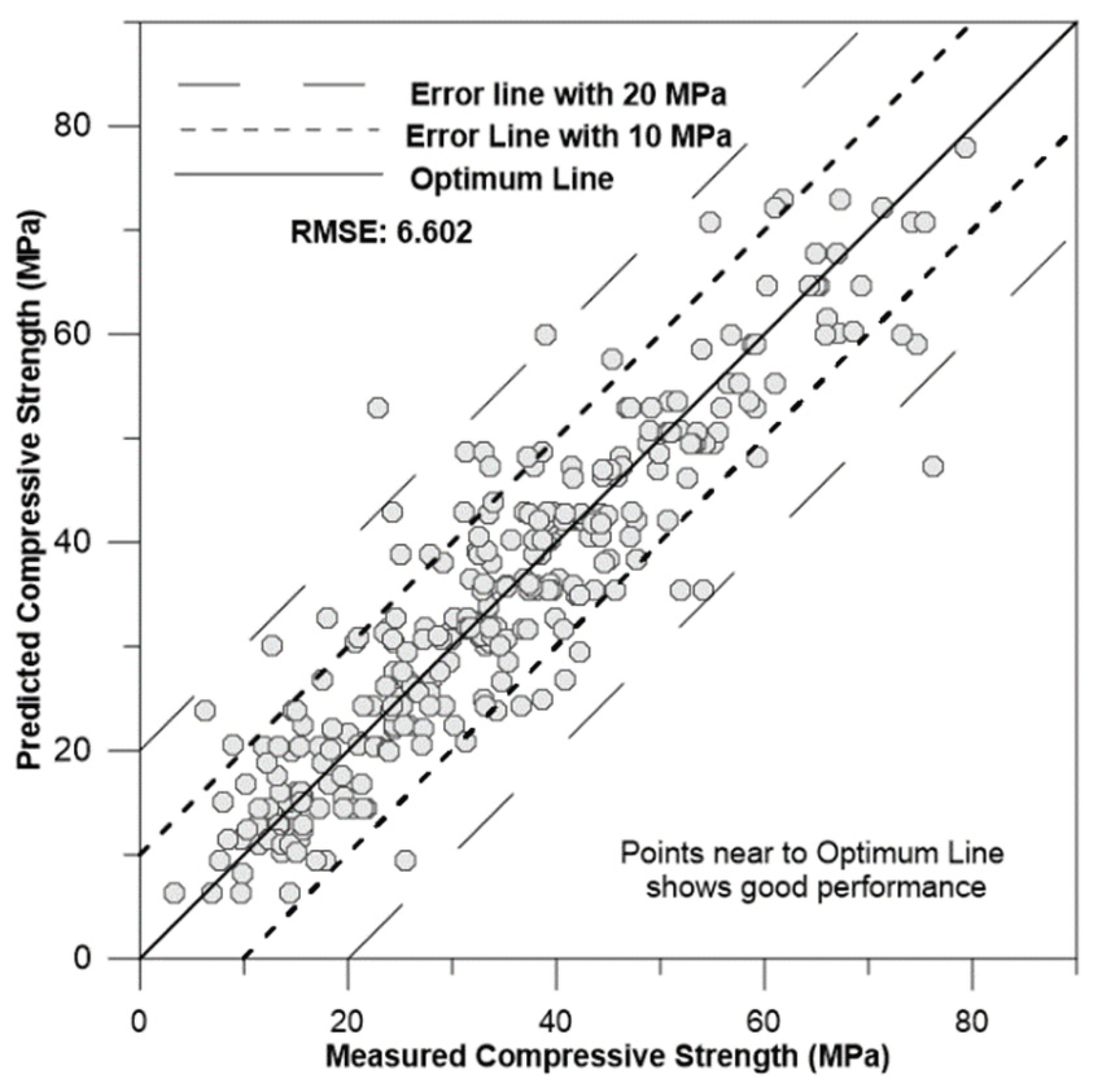
Upon reviewing the performance results of various models, it becomes evident that the ANN model outperforms the other models, as its RMSE and other values are the smallest in the table. The next best-performing model is SVM, which predicts with slightly less accuracy than the ANN model. Conversely, it can be concluded that the Multiple Regression model performs the worst under these conditions.
Figure 9,
Figure 10 and
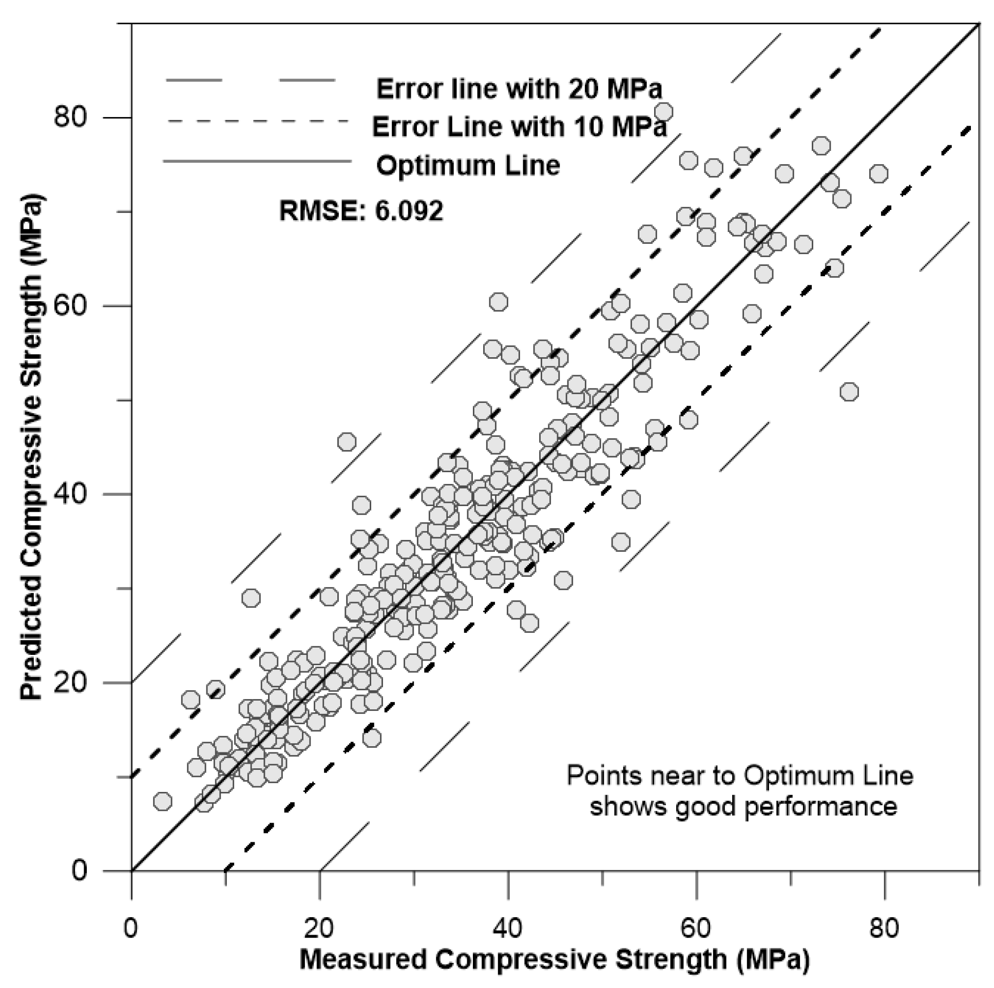
Figure 11 depicts the correlation of predicted concrete strength by different models to the measured concrete strength for simulated data.
4. Conclusion
The objective of this study was to streamline the process of predicting the compressive strength of concrete using various data-driven models such as Artificial Neural Networks (ANN), Support Vector Machines (SVM), Multiple Linear Regression (MLR), and Regression Trees. These methods were compared based on four different efficiency metrics. MATLAB software was employed for all calculations related to data-driven models due to its user-friendly interface, eliminating the need for advanced programming skills. The software’s intuitive design allows users to become familiar with basic tools and execute program steps sequentially.
This study utilized eight different variables to forecast the compressive strength of concrete, all of which are fundamental requirements in concrete manufacturing. In cases where certain items were not used in concrete production, a null value was employed in the prediction model. The results from all models demonstrated that the ANN model outperformed the other three models. This indicates that predicting the compressive strength of concrete can be more accurate and efficient using the ANN method, reducing the waiting period to determine concrete strength. By incorporating material weights during concrete production, the model provides strength results simultaneously with production, eliminating the need for specific equations or problem-solving methods.
The unique feature of retraining data and learning makes the ANN more suitable for prediction compared to other models. This study conducted an extensive comparison of the ANN model with three popular data prediction models, highlighting its importance in achieving high accuracy results. Additionally, this study offers a clear explanation of all parameters used in the ANN model, facilitating easy comprehension for future predictions.
Author Contributions
H.Y.M: Conceptualization, writing - review and editing, supervision, investigation, A.K.S: Data curation, writing - original draft preparation, methodology. All authors have read and agreed to the published version of the manuscript.
Funding
This research received no external funding.
Conflicts of Interest
The authors declare no conflicts of interest.
References
- Aiken, L. S., West, S. G., Pitts, S. C., Baraldi, A. N., & Wurpts, I. C. (2012). Multiple Linear Regression. In Handbook of Psychology, Second Edition. American Cancer Society. [CrossRef]
- Araiza-Aguilar, J. A., Rojas-Valencia, M. N., & Aguilar-Vera, R. A. (2020). Forecast generation model of municipal solid waste using multiple linear regression. Global Journal of Environmental Science and Management, 6(1), 1–14. [CrossRef]
- Boser, B. E., Guyon, I. M., & Vapnik, V. N. (1992). A training algorithm for optimal margin classifiers. Proceedings of the Fifth Annual Workshop on Computational Learning Theory, 144–152. [CrossRef]
- Brown, S. H. (2009). Multiple Linear Regression Analysis: A Matrix Approach with MATLAB. Alabama Journal of Mathematics, 34, 1–3.
- Campbell, C., & Ying, Y. (2022). Learning with Support Vector Machines. Springer Nature.
- Chou, J.-S., & Tsai, C.-F. (2012). Concrete compressive strength analysis using a combined classification and regression technique. Automation in Construction, 24, 52–60. [CrossRef]
- F, K., & K, B. (2016). Evaluation of Concrete Compressive Strength Using Artificial Neural Network And Multiple Linear Regression Models. 6(3), 423–432.
- Ji-Zong, W., Hong-Guang, N., & Jin-Yun, H. (1999). The application of automatic acquisition of knowledge to mix design of concrete. Cement and Concrete Research, 29(12), 1875–1880. [CrossRef]
- Jordan, M. I., & Mitchell, T. M. (2015). Machine learning: Trends, perspectives, and prospects. Science, 349(6245), 255–260. [CrossRef]
- Kaveh, A. (2002). Neural Networks for the Approximate Analysis and Design of Double Layer Grids. 17(1), 13. [CrossRef]
- Kohler, U., & Kreuter, F. (2005). Data Analysis Using Stata. Stata Press.
- Maind, S. B., & Wankar, P. (2014). Research Paper on Basic of Artificial Neural Network. International Journal on Recent and Innovation Trends in Computing and Communication, 2(1), 5.
- Mehta, P. K. (2002). Greening of the Concrete Industry for Sustainable Development. Concrete International, 24(7), 23–28.
- Moisen, G. G. (2008). Classification and regression trees. Encyclopedia of Ecology, 1, 582–588.
- Mr. Dongare Sadanand, Dr. Sachin Bhosale. (2023). Basic of Artificial Neural Network. International Journal of Advanced Research in Science, Communication and Technology, 299–303. [CrossRef]
- Neville, A. M. (2011). Properties of concrete (5th ed). Pearson.
- Özturan, M., Kutlu, B., & Özturan, T. (2008). COMPARISON OF CONCRETE STRENGTH PREDICTION TECHNIQUES WITH ARTIFICIAL NEURAL NETWORK APPROACH. 14.
- Sarker, I. H. (2021). Machine Learning: Algorithms, Real-World Applications and Research Directions. SN Computer Science, 2(3), 160. [CrossRef]
- Shevade, S. K., Keerthi, S. S., Bhattacharyya, C., & Murthy, K. R. K. (2000). Improvements to the SMO algorithm for SVM regression. IEEE Transactions on Neural Networks, 11(5), 1188–1193. [CrossRef]
- Smarzewski, P., & Stolarski, A. (2022). Properties and Performance of Concrete Materials and Structures. Crystals, 12(9), 1193. [CrossRef]
- Song, H., Ahmad, A., Farooq, F., Ostrowski, K. A., Maślak, M., Czarnecki, S., & Aslam, F. (2021). Predicting the compressive strength of concrete with fly ash admixture using machine learning algorithms. Construction and Building Materials, 308, 125021. [CrossRef]
- Ting, M.-K., Liao, P.-J., Wu, I.-W., Chen, S.-W., Yang, N.-I., Lin, T.-Y., & Hsu, K.-H. (2018). Predicting Type 2 Diabetes Mellitus Occurrence Using Three-Dimensional Anthropometric Body Surface Scanning Measurements: A Prospective Cohort Study. Journal of Diabetes Research, 2018, e6742384. [CrossRef]
- Yan, R., & Wang, S. (2022). Linear regression models. In Applications of Machine Learning and Data Analytics Models in Maritime Transportation (pp. 51–62). IET Digital Library. [CrossRef]
- Zupan, J. (1994). Introduction to Artificial Neural Network (ANN) Methods: What They Are and How to Use Them. Acta Chimica Slovenica, 41.
Figure 1.
Outline of 8-15-10-1 Architecture.
Figure 1.
Outline of 8-15-10-1 Architecture.
Figure 2.
ANN Model’s Best validation performance.
Figure 2.
ANN Model’s Best validation performance.
Figure 3.
Error histogram for all the steps of ANN.
Figure 3.
Error histogram for all the steps of ANN.
Figure 4.
Output Vs Target by ANN model for training data.
Figure 4.
Output Vs Target by ANN model for training data.
Figure 5.
Output Vs Target by ANN model for validation data.
Figure 5.
Output Vs Target by ANN model for validation data.
Figure 6.
Measured vs. Predicted compressive strength.
Figure 6.
Measured vs. Predicted compressive strength.
Figure 7.
Residual plot of SVM trained model.
Figure 7.
Residual plot of SVM trained model.
Figure 8.
Regression tree structure of the generated model.
Figure 8.
Regression tree structure of the generated model.
Figure 9.
Correlation of ANN predicted concrete strength to measured concrete strength for simulation data.
Figure 9.
Correlation of ANN predicted concrete strength to measured concrete strength for simulation data.
Figure 10.
Correlation of MLR predicted concrete strength to measured concrete strength for simulation data.
Figure 10.
Correlation of MLR predicted concrete strength to measured concrete strength for simulation data.
Figure 11.
Correlation of SVM predicted concrete strength to measured concrete strength for simulation data.
Figure 11.
Correlation of SVM predicted concrete strength to measured concrete strength for simulation data.
Figure 12.
Correlation of RT predicted concrete strength to measured concrete strength for simulation data.
Figure 12.
Correlation of RT predicted concrete strength to measured concrete strength for simulation data.
Table 1.
Dataset parameters and statistical value.
Table 1.
Dataset parameters and statistical value.
| Parameter |
Unit |
Mean |
Maximum |
Minimum |
Standard Deviation |
| Cement |
Kg/m3
|
281.166 |
540 |
102 |
104.507 |
| Blast Furnace Slag |
Kg/m3
|
73.895 |
359.4 |
0 |
86.279 |
| Fly Ash |
Kg/m3
|
54.187 |
200.1 |
0 |
63.996 |
| Water |
Kg/m3
|
181.566 |
247 |
121.75 |
21.356 |
| Superplasticizer |
Kg/m3
|
6.203 |
32.2 |
0 |
5.973 |
| Coarse Aggregate |
Kg/m3
|
972.919 |
1145 |
801 |
77.754 |
| Fine Aggregate |
Kg/m3
|
773.579 |
992.6 |
594 |
80.175 |
| Age |
Day |
45.662 |
365 |
1 |
63.170 |
| Concrete Compressive strength |
MPa |
35.818 |
82.599 |
2.332 |
16.706 |
Table 2.
Variance of different attributes.
Table 2.
Variance of different attributes.
| Attributes |
Variance |
| Cement |
10921.74 |
| Blast Furnace Slag |
7444.084 |
| Fly Ash |
4095.548 |
| Water |
456.0602 |
| Superplasticizer |
35.6826 |
| Coarse Aggregate |
6045.656 |
| Fine Aggregate |
6428.099 |
| Age |
3990.438 |
Table 3.
Correlation table.
Table 3.
Correlation table.
| Correlational coefficient |
Compressive Strength |
| Cement |
0.498 |
| Blast Furnace Slag |
0.135 |
| Fly Ash |
-0.106 |
| Water |
-0.29 |
| Superplasticizer |
0.366 |
| Coarse Aggregate |
-0.165 |
| Fine Aggregate |
-0.167 |
| Age |
0.329 |
| Compressive Strength |
1 |
Table 4.
Different ANN architecture model and their performance.
Table 4.
Different ANN architecture model and their performance.
| Architecture |
Value of R |
| Train |
Validation |
Test |
All |
| 8-10-1 |
0.96 |
0.91 |
0.93 |
0.95 |
| 8-20-1 |
0.96 |
0.92 |
0.93 |
0.95 |
| 8-15-1 |
0.96 |
0.96 |
0.97 |
0.96 |
| 8-20-10-1 |
0.97 |
0.94 |
0.87 |
0.95 |
Table 5.
Optimum parameter for the best-trained model.
Table 5.
Optimum parameter for the best-trained model.
| Network Properties |
|---|
| Parameter |
Value |
| Network Type |
Feed Forward Back Prop. |
| Training Function |
TRAINLM |
| Adaption Learning function |
LEARNGDM |
| Performance Function |
MSE |
| No. of Layer |
2(1-TANSIG, 2-TANSIG) |
| Number of neurons |
(1st Layer-15, 2nd layer-10) |
| Data division |
Random |
| Training |
Levenberg-Marquardt |
| Performance |
Mean Square Error |
| Calculation |
MEX |
Table 6.
Performance measurement of MLR Train data.
Table 6.
Performance measurement of MLR Train data.
| Model |
Training |
| MAD |
MSE |
RMSE |
MAPE |
| MLR |
3.6159 |
48.157 |
6.9395 |
13.2042 |
Table 7.
Result of different SVM trained model.
Table 7.
Result of different SVM trained model.
| SVM Model |
RMSE |
| Linear SVM |
10.966 |
| Quadratic SVM |
8.1616 |
| Cubic SVM |
6.9287 |
| Fine Gaussian SVM |
10.241 |
| Medium Gaussian SVM |
7.1213 |
| Coarse Gaussian SVM |
9.168 |
Table 8.
Result of different Regression Tree trained model.
Table 8.
Result of different Regression Tree trained model.
| Tree Model |
RMSE |
| Fine Tree |
7.5767 |
| Medium Tree |
8.2006 |
| Coarse Tree |
10.083 |
Table 9.
Performance measurement of Different Model.
Table 9.
Performance measurement of Different Model.
| Model |
Simulation |
| MAD |
CC |
RMSE |
MAPE |
| Artificial Neural Network(ANN) |
4.443 |
0.712 |
6.092 |
15.112 |
| Multiple linear regression(MLR) |
8.1824 |
-0.57 |
10.45 |
32.51 |
| Support vector machine(SVM) |
4.5813 |
0.724 |
6.3121 |
15.9816 |
| Regression tree |
4.6908 |
0.641 |
6.6029 |
17.6101 |
|
Disclaimer/Publisher’s Note: The statements, opinions and data contained in all publications are solely those of the individual author(s) and contributor(s) and not of MDPI and/or the editor(s). MDPI and/or the editor(s) disclaim responsibility for any injury to people or property resulting from any ideas, methods, instructions or products referred to in the content. |
© 2024 by the authors. Licensee MDPI, Basel, Switzerland. This article is an open access article distributed under the terms and conditions of the Creative Commons Attribution (CC BY) license (http://creativecommons.org/licenses/by/4.0/).

