Analyzing Bifurcations and Optimal Control Strategies in SIRS Epidemic Models: Insights from Theory and COVID-19 Data

Our study essentially concerns the dynamic behavior of an SIRS epidemic model in discrete time. Two equilibrium points are obtained; one is disease-free while the other is endemic. We are interested in the endemic fixed point as well as its asymptotic stability. Depending on the parameters which are estimated using the data from US Department of health and SIRS modelling with optimization, two Flip and Transcritical bifurcations appear. We illustrate their diagrams, as well as their bifurcation curves using the method of Carcasses \cite{carcasses1993determination,carcasses1995singularities} for the Flip bifurcation and by an implicit function deduced from such an equation for the Transcritical bifurcation. We use the scanning of the parametric plane to have a global view of the behavior of the model and to highlight the zones of stability of the existing singularities. A superposition of the bifurcation curves with the parametric plane can show the overlap of the curves with the boundaries of the stability domains, which confirms the smooth running of the simulation and its correspondence with the theory, we finish this article with constrained optimal control applied to infection rate and recruitment rate for an SIRS discrete epidemic model. Pontryagin's maximum principle is used to determine these optimal controls. Finally using COVID-19 data in the USA, we obtain results that demonstrate the effectiveness of the proposed control strategy to mitigate the spread of the pandemic.

Keywords:

Subject: Computer Science and Mathematics - Applied Mathematics

1. Introduction

The COVID-19 pandemic, caused by the SARS-CoV-2 virus, originated in Wuhan, China, in December 2019. It quickly spread globally, reaching North America where the first case was reported in Canada on January 23, 2020. Since then, three countries in North America (Canada, USA, and Mexico) have reported cases and deaths.

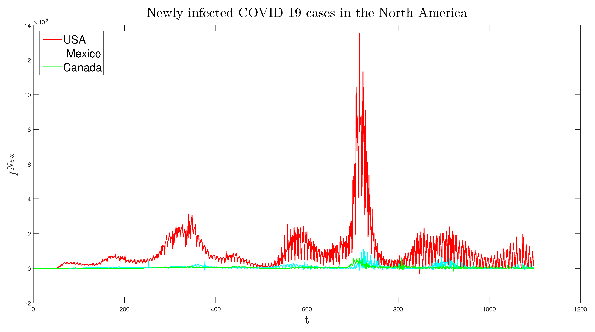
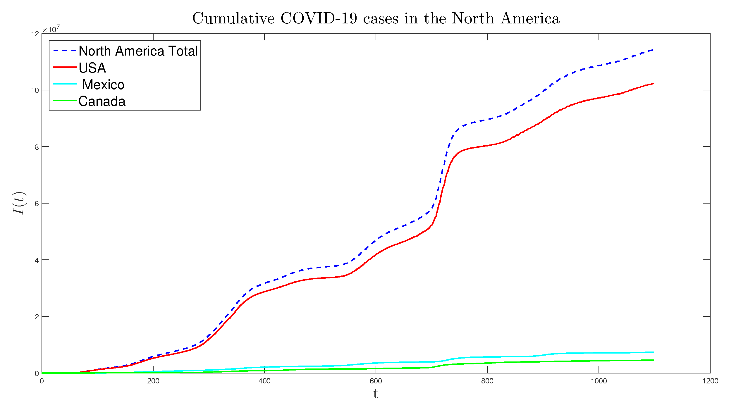
As of January 27, 2023, the total number of cases in North America stands at

114,196,623

, with the USA being the most severely impacted nation. Figure 1 and Figure 2 show the cumulative infected and newly infected Covid-19 cases from January 2020 to January 2023 of these North American countries.

The pandemic took a devastating toll on the United States, with the CDC confirming the first case of person-to-person transmission on January 30, 2020, and the HHS declaring it a Public Health Emergency on January 31, 2020. With

1,138,309

deaths overall, the USA has the highest death toll globally and ranks 20th highest per capita. It is the deadliest disaster in US history, ranking third in causes of death in 2020, after cancer and heart disease. Despite constituting

67 %

of North America’s population, the USA accounted for approximately

90 %

of the total cumulative COVID-19 cases in the region as of January 27, 2023 1.

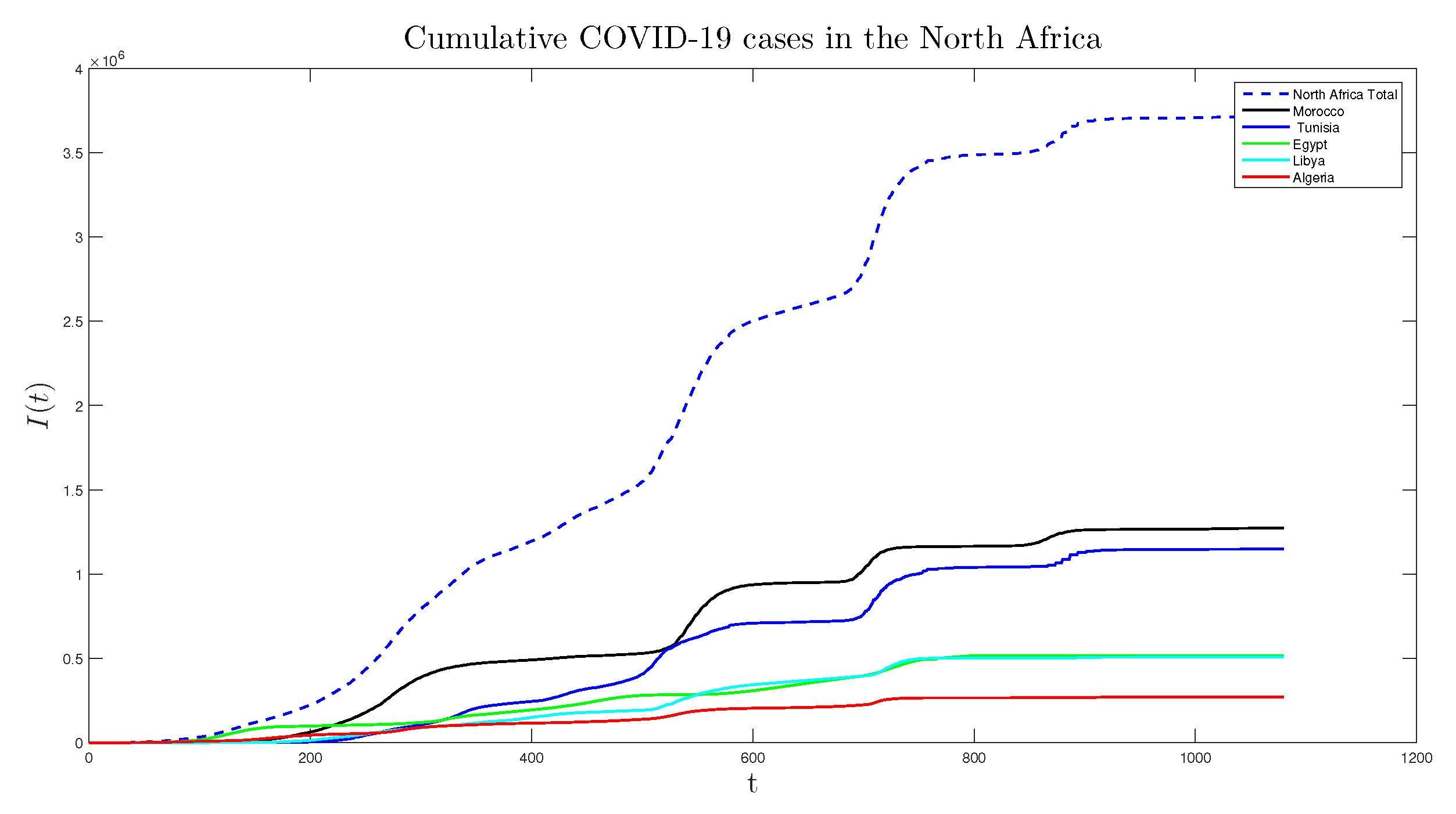
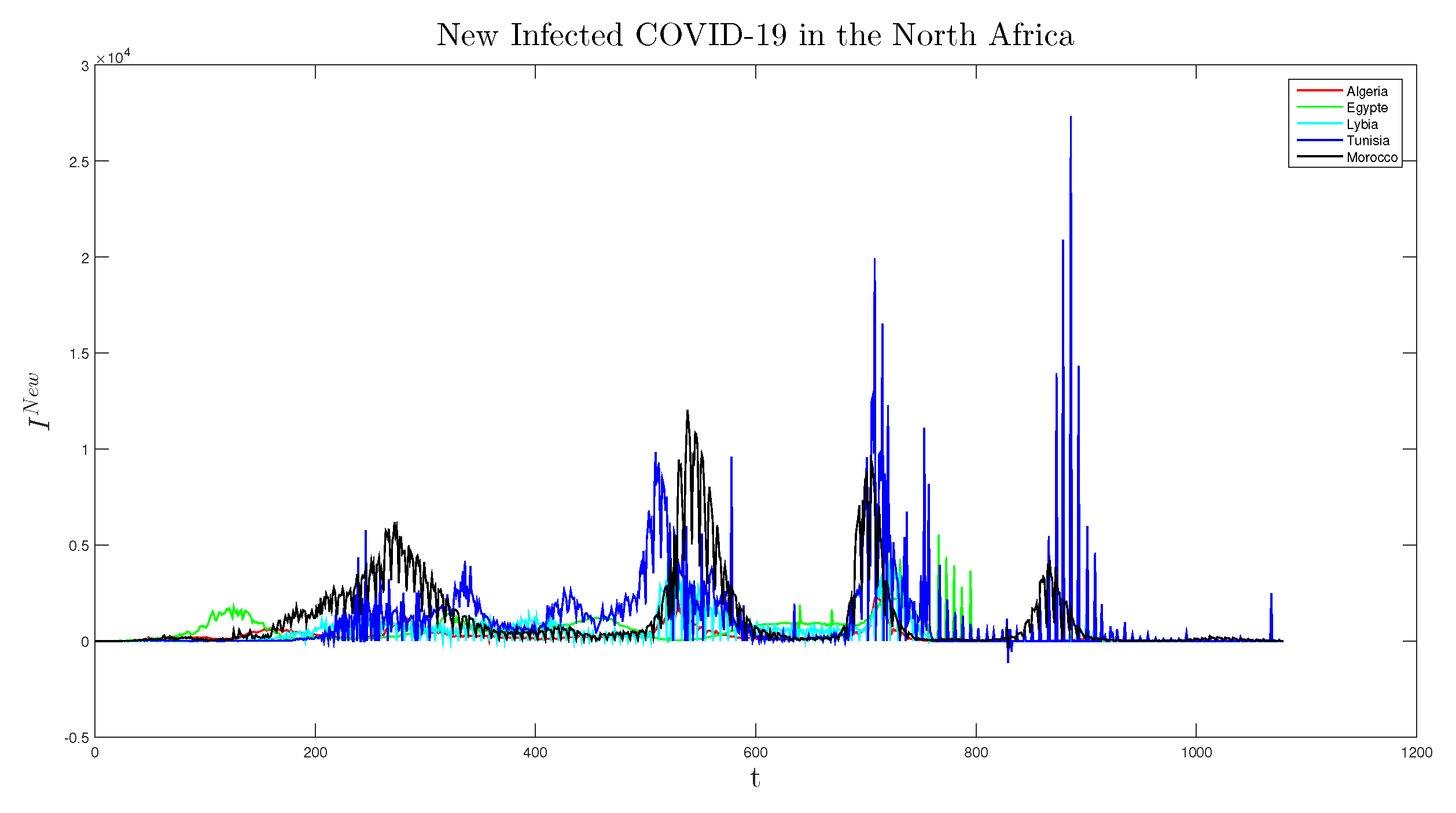
Similarly, in Africa, the first case of COVID-19 was reported in North Africa, specifically in Egypt, on February 14, 2020. Since then, five countries in North Africa (Algeria, Egypt, Libya, Morocco, and Tunisia) have reported cases and deaths. As of January 27, 2023, the total number of cases in North Africa stands at

3,716,668

, with Tunisia and Morocco being the most severely impacted nations. Figure 3 and Figure 4 show the cumulative infected and newly infected Covid-19 cases from January 2020 to January 2023 of these North Africa countries.

The largest country in Africa, Algeria, managed to protect itself from the virus through swift government responses, including the closure of borders and travel restrictions between provinces. Despite constituting

21.40 %

of North Africa’s population, Algeria accounted for approximately

10 %

of the total cumulative COVID-19 cases in the region as of January 27, 2023.

The parameters used in our study are estimated by optimization using Python. In this study, all simulations and graphics were performed using Python, Matlab, and Fortran.

In this paper, we use the COVID-19 pandemic model to illustrate bifurcation in an SIRS model. In the early stages of the pandemic, the disease-free equilibrium was stable, meaning that the virus could not spread widely. However, as the virus mutated and became more transmissible, the basic reproduction number

R_{0}

crossed 1 and the disease-free equilibrium became unstable. This led to a transcritical bifurcation, which resulted in a rapid and widespread outbreak of COVID-19.

Furthermore, this contribution emphasizes the application of optimal control theory to devise strategies that effectively mitigate virus transmission within a SIRS model. This involves selecting appropriate values for control variables to minimize specific objective functions, such as the total number of infected individuals or the peak number of infected individuals.

The paper is structured as follows: Section 2 introduces a biological model described by discrete-time equations. Section 3 estimates the model parameters for Algeria and the USA. Section 4 examines the stability and existence of fixed points and their stability analysis. Section 5 conducts a bifurcation analysis, while Section 6 delves into the study of an optimal control problem. Section 8 presents numerical simulations to validate the obtained results, finally, these results are discussed, and conclusions are made in Section 9.

2. The Model

Numerous scientists are attempting to investigate COVID-19’s behavior from a mathematical perspective, the author applied modified SIR (susceptible, infected, and recovered), and SIRS (susceptible, infected, recovered, and susceptible) models to estimate the current COVID-19 infection rate based on several methods for controlling the virus’s rapid spread. Many mathematicians talk about this Covid-19 in various dynamic models [3]: in continious [4,5] and discret [6,7] time also with stochastic modeling [8,9].

Numerous studies have already looked into the discrete-time epidemic models. Lee and Wong [10] spoke about the bifurcation analysis and other dynamical phenomena of SIR epidemic model, which is essentially a differential equations epidemic model [11], is described as follows:

\{\begin{matrix} \frac{d S}{d t} = A - μ S - λ S I + β R, \\ \frac{d I}{d t} = λ S I - (μ + r) I, \\ \frac{d R}{d t} = r I - (μ + β) R, \\ N (t) = S (t) + I (t) + R (t) . \end{matrix}

(1)

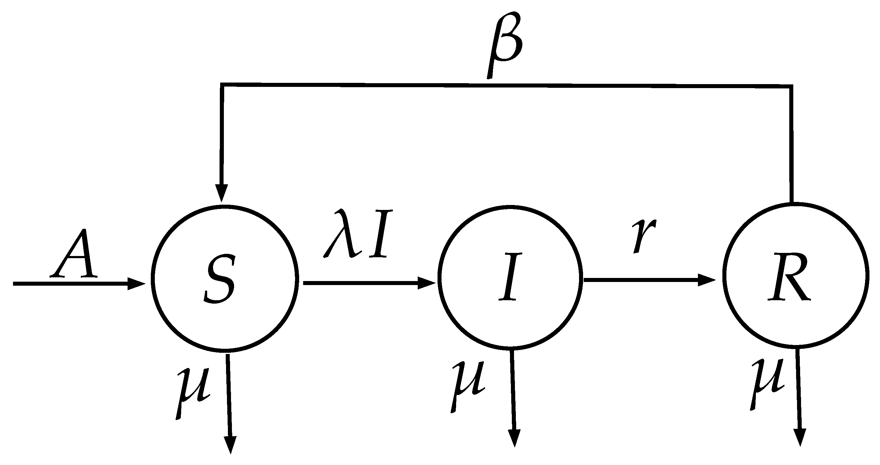
where

S (t), I (t), R (t)

and

N (t)

denote the numbers of susceptible, infective, recovered individuals and total numbers of the individuals at time t , respectively, A is the recruitment rate of the population,

μ

is the natural death rate of the population, r is the recovery rate of the infective individuals,

λ

is the bilinear incidence rate and

β

is the rate of loss of immunity, we draw up a flow transmission diagram between the three different classes (Figure 5).

Applying the forward Euler scheme to model (1), we obtain the following discrete-time SIR epidemic model

\{\begin{matrix} S_{n + 1} = F (S_{n}, I_{n}, R_{n},) : = S_{n} + h (A - μ S_{n} - λ S_{n} I_{n} + β R_{n}), \\ I_{n + 1} = G (S_{n}, I_{n}, R_{n},) : = I_{n} + h (λ S_{n} I_{n} - (μ + r) I_{n}), \\ R_{n + 1} = H (S_{n}, I_{n}, R_{n},) : = R_{n} + h (r I_{n} - (μ + β) R_{n}), \\ N_{n + 1} = (1 - h μ) N_{n} + h A, \end{matrix}

(2)

where h is the step size. It is assumed that

S (0) \geq 0, I (0) \geq 0, R (0) \geq 0

, and all the parameters

A, h, r, β, λ

and

μ

are positive constants. The dynamical behaviors of the model (2) are equivalent to the dynamical behaviors of the map

T : R^{3} ⟶ R^{3}

, written in the recurrence form:

\begin{matrix} (S_{n + 1}, I_{n + 1}, R_{n + 1}) & = T (S_{n}, I_{n}, R_{n}) \\ : = (F (S_{n}, I_{n}, R_{n}), G (S_{n}, I_{n}, R_{n}), H (S_{n}, I_{n}, R_{n})) \end{matrix}

(3)

3. Data and Parameter Identification (Materials and Methods)

The COVID-19 information used in this study was obtained from 2. The data were dated from May 10, 2021, to September 5, 2021 for Algeria and from October 24, 2021, to March 10, 2022 for USA. The data is preprocessed, including calculating new infected cases and new recovered cases from cumulative data, applying a smoothing filter (savgol_filter), and adjusting demographics data.

Model Fitting

To optimize the parameters (

r, λ

and

β

) of the model we developed a code which uses the minimization method to adjust the parameters of the SIRS model to the observed epidemiological data. The objective function used to minimize is defined as the sum of the squared deviations between the observed data and the model predictions. Figures (Figure 6 and Figure 7) show data for new infected and new recovered, as well as comparisons between observed data and model predictions for both countries Algeria and USA.

Numerical simulation were carried out to provide a clearer picture regarding stability region on the

(A, λ)

-parameter plan while fixing the values of parameter

h = 0.1

β

, and r as specified in Table 1 corresponding to USA, and

μ = 0.0082

Next, we explore the existence, stability and types of equilibria for system (3).

4. Analysis of Equilibria

Applying next-generation matrix approach [12], we compute basic reproduction number as:

R_{0} = {\frac{\partial (λ S I)}{\partial I} \times {(\frac{\partial [(μ + r) I]}{\partial I})}^{- 1}|}_{(S, I, R) = (\frac{A}{μ}, 0, 0)} = \frac{A λ}{μ (μ + r)},

which represents the average amount of subsequent infections produced by an initial group of infected individuals over their lifetime. Concerning the existence of non-negative equilibrium points for system (3), we present the following results:

Theorem 1.

System (3) always has a disease-free equilibrium

E_{0} = (\frac{A}{μ}, 0, 0)

. Moreover,

if $R_{0} < 1$ , then the model (3) has only disease-free equilibrium $E_{0}$ .
if $R_{0} > 1$ , then the model (3) has also an endemic equilibrium, given by

$E_{1} = (\frac{μ + r}{λ}, \frac{(A λ - μ (μ + r)) (β + μ)}{μ λ (β + μ + r)}, \frac{r (A λ - μ (μ + r))}{μ λ (β + μ + r)}) .$

Proof.

The equilibrium

E = (S, I, R)

of system (3) satisfies

\{\begin{matrix} A - (μ + λ I) S + β R = 0, \\ [λ S - (μ + r)] I = 0, \\ r I - (μ + β) R = 0 . \end{matrix}

(4)

From the second equation of the system (3), we obtain

I = 0

λ S - (μ + r) = 0

, so

E_{0} = (\frac{A}{μ}, 0, 0)

. On the other hand,

λ S - (μ + r) = 0

and the condition on I and

R (I_{n} \geq 0, R_{n} \geq 0

, for all n), we have

E_{1} = (\frac{μ + r}{λ}, \frac{(A λ - μ (μ + r)) (β + μ)}{μ λ (β + μ + r)}, \frac{r (A λ - μ (μ + r))}{μ λ (β + μ + r)})

\frac{A λ}{μ (μ + r)} > 1

. □

In the context of the discrete system (3), the stability analysis involves linearizing the system around an equilibrium point

(S^{*}, I^{*}, R^{*})

by calculating the Jacobian matrix

J (S^{*}, I^{*}, R^{*}) = [\begin{matrix} 1 - h (I^{*} λ + μ) & - h λ S^{*} & h β \\ h λ I^{*} & 1 + h (λ S^{*} - (μ + r)) & 0 \\ 0 & h r & 1 - h (β + μ) \end{matrix}] .

and evaluating it at the equilibrium point. The eigenvalues of this Jacobian matrix are crucial in determining stability. If all eigenvalues of

J (S^{*}, I^{*}, R^{*})

have absolute values less than 1, the equilibrium point is asymptotically stable. If at least one eigenvalue has an absolute value greater than 1, the equilibrium point is unstable. The specific values of the parameters

(A, μ, λ, β, r)

and the equilibrium values

(S^{*}, I^{*}, R^{*})

will determine the stability of the system. This analysis is typically carried out numerically, as finding analytical solutions might be challenging for nonlinear systems. Nevertheless, we can sometimes establish some analytical results as follows.

Theorem 2.

(1)

If the basic reproduction rate

R_{0} < 1

. Then

(a): $E_{0}$ is a stable node (sink) if

$0 < h < h_{*} = 2 min \{\frac{1}{μ + β}, \frac{1}{(μ + r) (1 - R_{0})}\}$ ,
(b): $E_{0}$ is a unstable node (source) if

$h > h^{*} = 2 max \{\frac{1}{μ}, \frac{1}{(μ + r) (1 - R_{0})}\}$ ,
(c): $E_{0}$ is non-hyperbolic if

$h \in \{\frac{2}{μ}, \frac{2}{μ + β}, \frac{2}{(μ + r) (1 - R_{0})}\}$ ,
(d): $E_{0}$ is a saddle if

$h_{*} < h < h^{*}$ and $h \notin \{\frac{2}{μ}, \frac{2}{μ + β}, \frac{2}{(μ + r) (1 - R_{0})}\}$ .

(2)

If the basic reproduction rate

R_{0} > 1

(a): $E_{0}$ is a unstable node (source) if

$h > \frac{2}{μ}$ ,
(b): $E_{0}$ is non-hyperbolic if

$h \in \{\frac{2}{μ}, \frac{2}{μ + β}\}$ ,
(c): $E_{0}$ is a saddle if

$h < \frac{2}{μ}$ and $h \neq \frac{2}{μ + β}$ .

Proof.

Jacobian matrix of model (3) at

E_{0}

J (E_{0}) = [\begin{matrix} - μ h + 1 & - h λ \frac{A}{μ} & h β \\ 0 & 1 + h (\frac{λ A}{μ} - μ - r) & 0 \\ 0 & h r & 1 - h (β + μ) \end{matrix}] .

The result follows from the calculation of the eigenvalues of the matrix

J (E_{0})

, i.e.,

ω_{1} = 1 - h μ, ω_{2} = 1 + h \frac{A λ - μ (μ + r)}{μ}

and

ω_{3} = 1 - h (β + μ)

(1)

If the basic reproduction rate

R_{0} < 1

. Then

(a): $E_{0}$ is a stable node (sink) if

$|ω_{1}| < 1, |ω_{2}| < 1$ and $|ω_{3}| < 1 ⟹ 0 < h < \frac{2}{μ}, 0 < h < \frac{2 μ}{μ (μ + r) - A λ}$ and $0 < h < \frac{2}{μ + β} ⟹ 0 < h < h_{*} = 2 m i n \{\frac{1}{μ + β}, \frac{1}{(μ + r) [1 - R_{0}]}\}$
(b): $E_{0}$ is a unstable node (source) if

$|ω_{1}| > 1, |ω_{2}| > 1$ and $|ω_{3}| > 1 ⟹ h > \frac{2}{μ}, h > \frac{2 μ}{μ (μ + r) - A λ}$ and $h > \frac{2}{μ + β} ⟹ h > h^{*} = 2 m a x \{\frac{1}{μ}, \frac{1}{(μ + r) [1 - R_{0}]}\}$
(c): $E_{0}$ is non-hyperbolic if

$|ω_{1}| = 1$ or $|ω_{2}| = 1$ or $|ω_{3}| = 1 ⟹ h = \frac{2}{μ}$ or $h = \frac{2 μ}{μ (μ + r) - A λ}$ or $h = \frac{2}{μ + β} ⟹ h \in \{\frac{2}{μ}, \frac{2}{μ + β}, \frac{2}{(μ + r) (1 - R_{0})}\}$ ,
(d): $E_{0}$ is a saddle if

$(|ω_{1}| < 1 \land |ω_{2}| < 1 \land |ω_{3}| > 1)$ or $(|ω_{1}| < 1 \land |ω_{2}| > 1 \land |ω_{3}| > 1)$

or $(|ω_{1}| < 1 \land |ω_{2}| > 1 \land |ω_{3}| < 1)$ or $(|ω_{1}| > 1 \land |ω_{2}| < 1 \land |ω_{3}| < 1)$

or $(|ω_{1}| > 1 \land |ω_{2}| < 1 \land |ω_{3}| > 1)$ or $(|ω_{1}| > 1 \land |ω_{2}| > 1 \land |ω_{3}| < 1) ⟶ h_{*} < h < h^{*}$ and $h \notin H = \{\frac{2}{μ}, \frac{2}{μ + β}, \frac{2}{(μ + r) [1 - R_{0}]}\}$ .

(2)

If the basic reproduction rate

R_{0} > 1

(a): $E_{0}$ is a stable node (sink) if

$h < h_{*} = 2 min \{\frac{1}{μ + β}, \frac{1}{(μ + r) (1 - R_{0})}\} ⟶ h < \frac{1}{(μ + r) (1 - R_{0})} < 0$ impossible
(b): $E_{0}$ is a unstable node (source) if

$|ω_{1}| > 1, |ω_{2}| > 1$ and $|ω_{3}| > 1 ⟹ h > \frac{2}{μ}, h > \frac{2 μ}{μ (μ + r) - A λ}$ and $h > \frac{2}{μ + β} ⟹ h > h^{*} = \frac{1}{μ}$ ,
(c): $E_{0}$ is non-hyperbolic if

$|ω_{1}| = 1$ or $|ω_{2}| = 1$ or $|ω_{3}| = 1 ⟹ h = \frac{2}{μ}$ or $h = \frac{2 μ}{μ (μ + r) - A λ}$ or $h = \frac{2}{μ + β} ⟹ h \in \{\frac{2}{μ}, \frac{2}{μ + β}\}$ ,
(d): $E_{0}$ is a saddle if

$(|ω_{1}| < 1 \land |ω_{2}| < 1 \land |ω_{3}| > 1)$ or $(|ω_{1}| < 1 \land |ω_{2}| > 1 \land |ω_{3}| > 1)$

or $(|ω_{1}| < 1 \land |ω_{2}| > 1 \land |ω_{3}| < 1)$ or $(|ω_{1}| > 1 \land |ω_{2}| < 1 \land |ω_{3}| < 1)$

or $(|ω_{1}| > 1 \land |ω_{2}| < 1 \land |ω_{3}| > 1)$ or $(|ω_{1}| > 1 \land |ω_{2}| > 1 \land |ω_{3}| < 1) ⟶ h < \frac{2}{μ}$ and $h \neq \frac{2}{μ + β}$ .

□

The following result on the local stability of disease-free equilibrium

E_{0} = (\frac{A}{μ}, 0, 0)

can be obtained simply from Theorem 2.

Corollary 1.

(1): When $R_{0} < 1$ , if $0 < h < h_{*}$ then disease-free equilibrium $E_{0} = (\frac{A}{μ}, 0, 0)$ is locally asymptotically stable and if $h > h_{*}$ then disease-free equilibrium $E_{0} = (\frac{A}{μ}, 0, 0)$ is unstable.
(2): When $R_{0} > 1$ , we have that disease-free equilibrium $E_{0} = (\frac{A}{μ}, 0, 0)$ is always unstable.

Jacobian matrix of model (3) at

E_{1}

J (E_{1}) = [\begin{matrix} 1 + h (- \frac{(μ + β) (A λ - μ^{2} - μ r)}{μ (β + μ + r)} - μ) & - h (r + μ) & h β \\ \frac{h (μ + β) (A λ - μ^{2} - μ r)}{μ (β + μ + r)} & 1 & 0 \\ 0 & h r & 1 - h (β + μ) \end{matrix}]

We obtain three eigenvalues of

J (E_{1})

are

ω_{1}, ω_{2}

and

ω_{3}

given by

\{\begin{matrix} ω_{1} = 1 - h μ, \\ ω_{2} = - \frac{1}{2 μ (β + μ + r)} [a + \sqrt{Δ}], \\ ω_{3} = - \frac{1}{2 μ (β + μ + r)} [a - \sqrt{Δ}] . \end{matrix}

(5)

where

\{\begin{matrix} a = A h λ (β + μ) + μ (bh (β + μ) - 2 (β + μ + r)) \\ b_{1} = λ^{2} A^{2} (β + μ) \\ b_{2} = 2 λ A (β (β + (3 μ + 4 r)) + 2 μ (μ + 2 r) + 2 r^{2}) \\ b_{3} = μ^{2} (β (β (β + 5 μ + 4 r) + 8 μ ((μ + 2 r) + r^{2}))) \\ b_{4} = 4 (μ (μ (μ + 3 r) + 3 r^{2}) + r^{3}) \\ Δ = h^{2} (β + μ) (b_{1} - b_{2} + b_{3} + b_{4}) \end{matrix}

Theorem 3.

Let

R_{0} > 1

, the endemic equilibrium

E_{1}

is a sink, if one of the following conditions holds

(a): $Δ \geq 0$ and the eigenvalues $w_{2, 3}$ satisfy $- 1 \leq w_{2, 3} \leq 1$ .
(b): $Δ \geq 0$ and the conjugate complex eigenvalues $w_{2, 3}$ satisfy $|w_{2, 3}| < 1$ .

5. Bifurcation Analysis

Bifurcation is a qualitative or quantitative change in the dynamics that occurs when a parameter of the model crosses a critical threshold. This can lead to major shifts in the course of an epidemic, such as the transition from a controlled outbreak to a major pandemic. By understanding the conditions that lead to bifurcations, and the biological implications of these events, it is possible to develop more effective control strategies for infectious diseases. In this section, we investigate in detail the bifurcation structures of the SIR system (1) in the

(A, λ)

two-dimensional parameters space. We will make use of the classical fold and flip bifurcations. We study the behavior of such curves related to some cycles of order

k \in N

. For more details about bifurcation theory see for example [13,14].

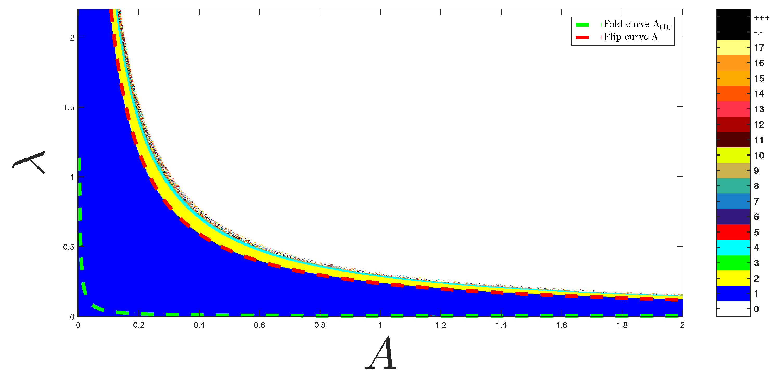
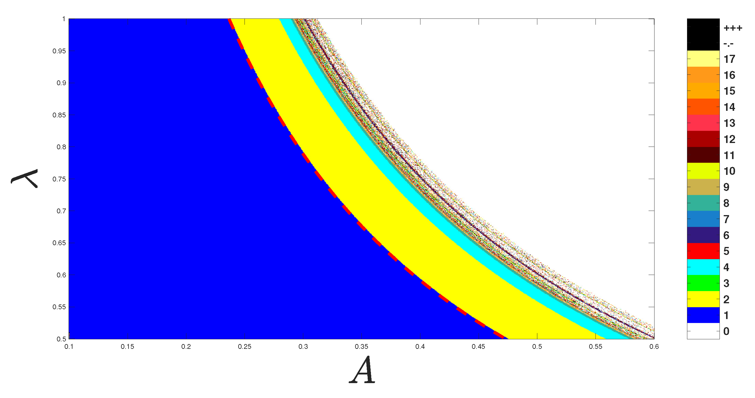
Figure 8 represents the stability domains obtained by numerical simulations for the transformation (1) in the parameter plane

(A, λ)

for

h = 0.1, β = 1.16743084, μ = 0.0082

and

r = 0.07714

, respectively. Each colored region corresponds to the existence of a stable periodic orbit with a period indicated in the bar on the right of the figure. When A is changed, we can remark that some stability regions are periodically repeated (Figure 9, Figure 10 and Figure 11).

Figure 8 represent the stability domains obtained by numerical simulations for the transformation (1) in the parameter plane

(A, λ)

for

h = 0.1, β = 1.16743084, μ = 0.0082

and

r = 0.07714

, respectively.

5.1. Bifurcation Curve

Analytical methods can be used to derive bifurcation curves for fixed points and periodic cycles in dynamical systems based on the concept of reduced multiplier introduced in [1,2]. Let

X^{*} = (S^{*}, I^{*}, R^{*}) \in R^{3}

be a k-cycle, The characteristic equation (written for

T^{k}

) associated with this cycle can be expressed as follows: The reduced multiplier linked to this cycle is the real number

σ

that satisfies the equation

\sum (σ, S^{*}, I^{*}, R^{*}) : = (J_{T^{k}} (X^{*})) + det (J_{T^{k}} (X^{*})) - σ (1 + M_{S} + M_{I} + M_{R}) = 0

, where det and denote the determinant and trace of the matrix, respectively.

J_{T} (X^{*}) = [\begin{matrix} \frac{\partial F^{k} (S, I, R)}{\partial S} & \frac{\partial F^{k} (S, I, R)}{\partial I} & \frac{\partial F^{k} (S, I, R)}{\partial R} \\ \frac{\partial G^{k} (S, I, R)}{\partial S} & \frac{\partial G^{k} (S, I, R)}{\partial I} & \frac{\partial G^{k} (S, I, R)}{\partial R} \\ \frac{\partial H^{k} (S, I, R)}{\partial S} & \frac{\partial H^{k} (S, I, R)}{\partial I} & \frac{\partial H^{k} (S, I, R)}{\partial R} \end{matrix}]

and the three determinants

M_{S}, M_{I}

and

M_{R}

, built up from the minors of the Jacobian matrix

J_{T} (X^{*})

, are

M_{S} = det ([\begin{matrix} \frac{\partial G^{k} (S, I, R)}{\partial I} & \frac{\partial G^{k} (S, I, R)}{\partial R} \\ \frac{\partial H^{k} (S, I, R)}{\partial I} & \frac{\partial H^{k} (S, I, R)}{\partial R} \end{matrix}])

M_{I} = det ([\begin{matrix} \frac{\partial F^{k} (S, I, R)}{\partial S} & \frac{\partial F^{k} (S, I, R)}{\partial R} \\ \frac{\partial H^{k} (S, I, R)}{\partial S} & \frac{\partial H^{k} (S, I, R)}{\partial R} \end{matrix}])

and

M_{R} = det ([\begin{matrix} \frac{\partial F^{k} (S, I, R)}{\partial S} & \frac{\partial F^{k} (S, I, R)}{\partial I} \\ \frac{\partial G^{k} (S, I, R)}{\partial S} & \frac{\partial G^{k} (S, I, R)}{\partial I} \end{matrix}])

. The bifurcations are studied in the

(A, λ)

parameter plane in the case of k-cycles, then the evolution of the bifurcation structure in this plane will be studied by varying the parameters A and

λ

Theorem 4.

For the map (2), a fold bifurcation curve of order k (i.e., related to k-cycle of T) denoted as

Λ_{(k) 0}

in the

(A, λ)

-plane is the solution of the system

\{\begin{matrix} F^{k} (S, I, R; A, λ) = S, \\ G^{k} (S, I, R; A, λ) = I, \\ H^{k} (S, I, R; A, λ) = R, \\ Σ (1, S, I, R, A, λ) = 0 . \end{matrix}

(6)

Theorem 5.

For the map (2), a flip bifurcation curve of order k (i.e., related to k-cycle of T) denoted as

Λ_{k}

in the

(A, λ)

-plane is the solution of the system

\{\begin{matrix} F^{k} (S, I, R; A, λ) = S, \\ G^{k} (S, I, R; A, λ) = I, \\ H^{k} (S, I, R; A, λ) = R, \\ Σ (- 1, S, I, R, A, λ) = 0 . \end{matrix}

(7)

5.1.1. Flip Bifurcation

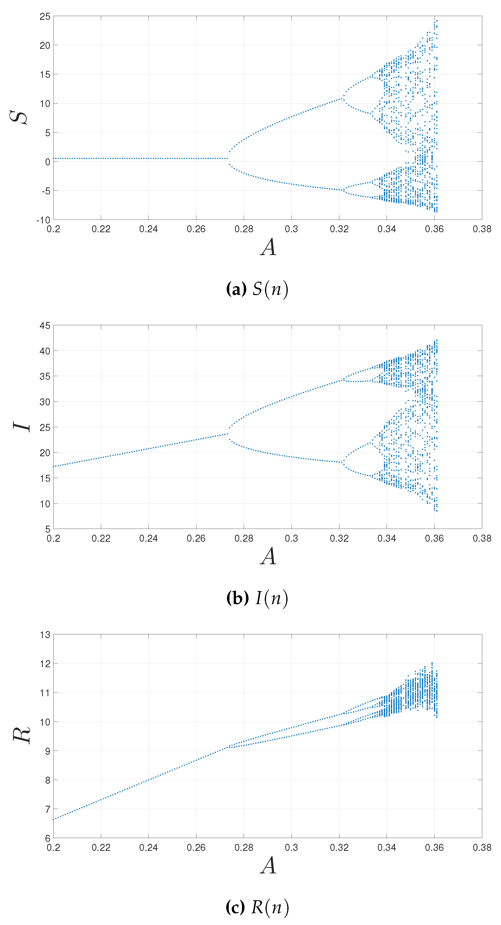
A period doubling bifurcation in discrete dynamical systems is a type of bifurcation in which the period of the model’s oscillations doubles. This can happen when a parameter of the model, such as the transmission rate, is gradually increased. At a certain critical value of the parameter, the model will transition from a state in which it oscillates with a period of

k = 1

to a state in which it oscillates with a period of

k = 2

. This can continue to happen, with the period doubling each time, until the model reaches a chaotic state. Period doubling bifurcations are important in SIR models because they can lead to unpredictable and erratic behavior in the spread of the disease. For example, a period of doubling bifurcation could lead to a sudden and unexpected increase in the number of infected individuals, even if the transmission rate of the disease has not changed significantly. When a stable cycle of order k has an eigenvalue that passes through the value

- 1

, a bifurcation of this type occurs. After that, this cycle destabilizes and gives rise to a stable cycle of order

2 k

. The equation of a Flip bifurcation curve for a fixed point

E_{1}

λ = \frac{μ ((μ + β) (μ + r) (μ + r + β) h^{2} + 2 β (μ + β) h - 4 d - 4 r - 4 β)}{A (μ + β) h (- 2 + (μ + r + β) h)}

5.1.2. Transcritical Bifurcation

This bifurcation is equivalent to the meeting of two fixed points

E_{0}

and

E_{1}

with opposing stability, which merge to form a saddle fixed point before separating once more by exchanging their stability. The equation of a trans-critical bifurcation curve is

R_{0} = 1

, i.e.

A λ - μ (μ + r) = 0

5.2. Numerical Simulation

To illustrate the results presented above, we give numerical simulations in this section.

5.2.1. Flip Bifurcation (or Period Doubling Bifurcation)

A period-doubling bifurcation in discrete dynamical systems is a type of bifurcation in which the period of the model’s oscillations doubles. This can happen when a parameter of the model, such as the transmission rate, is gradually increased. At a certain critical value of the parameter

h \approx 2.9

, the model will transition from a state in which it oscillates with a period of

k = 1

to a state in which it oscillates with a period of

k = 2

. This can continue to happen, with the period doubling each time, until the model reaches a chaotic state. Period doubling bifurcations are important in SIR models because they can lead to unpredictable and erratic behavior in the spread of the disease. For example, a period of doubling-bifurcation could lead to a sudden and unexpected increase in the number of infected individuals, even if the transmission rate of the disease has not changed significantly.

5.2.2. Transcritical Bifurcation

In a transcritical bifurcation, our two fixed points

E_{0}

and

E_{1}

have opposite stabilities and exchange their stabilities in

(A, λ) = (A^{*}, λ^{*})

6. The Optimal Control Problem

To reduce the number of vulnerable and infectious people with the least amount of expenditure on disease control, we apply the best control measures, such as confinement, vaccination, and border control. The primary goal of this section is to propose a way to handle this particular type of optimization issue. Two control variables are used to formulate this problem as an optimal control problem (that represents border control and treatment strategies). We now present two controls u and v which control new immigrants arriving from abroad and infected people receiving treatment, respectively, per unit of time, so that (1) becomes:

\{\begin{matrix} \frac{d S}{d t} = u A - μ S - v λ S I + β R, \\ \frac{d I}{d t} = v λ S I - (μ + r) I, \\ \frac{d R}{d t} = r I - (μ + β) R, \\ N (t) = S (t) + I (t) + R (t) . \end{matrix}

(8)

\{\begin{matrix} d S = (A - d S - λ S I + β R) d t + σ_{1} d B (t), \\ d I = (λ S I - (d + r) I) d t + σ_{2} d B (t), \\ d R = (r I - (d + β) R) d t, \end{matrix}

(9)

Where dB(t) is the independent standard Brownian motions and

σ_{1}

and

σ_{2}

are the intensities of white noises.

7. SDE with Optimal Control

In this section of the investigation, we employ control theory instruments to limit the spread of COVID-19. Using the control variables u and v for models (9), we have the following optimal strategy for the stochastic model. We will take into consideration system (9) together with two control measures, u, and v, to construct a control mechanism for reducing COVID-19. The goal of the plan is to minimize the following functional

J (u, v) = E (\int_{0}^{T} (\frac{1}{2} u_{t}^{2} + \frac{1}{2} v_{t}^{2} + I_{t}) d t)

Model (8) assumes the form by considering the controls.

\{\begin{matrix} d S = (u A - d S - v λ S I + β R) d t + σ_{1} d B (t), \\ d I = (v λ S I - (d + r) I) d t + σ_{2} d B (t), \\ d R = (r I - (μ + β) R) d t, \end{matrix}

(10)

The problem is to minimize the cost functional given by:

J (u, v) = \int_{0}^{T} (\frac{1}{2} u_{s}^{2} + \frac{1}{2} v_{s}^{2} + I_{s}) d s

(11)

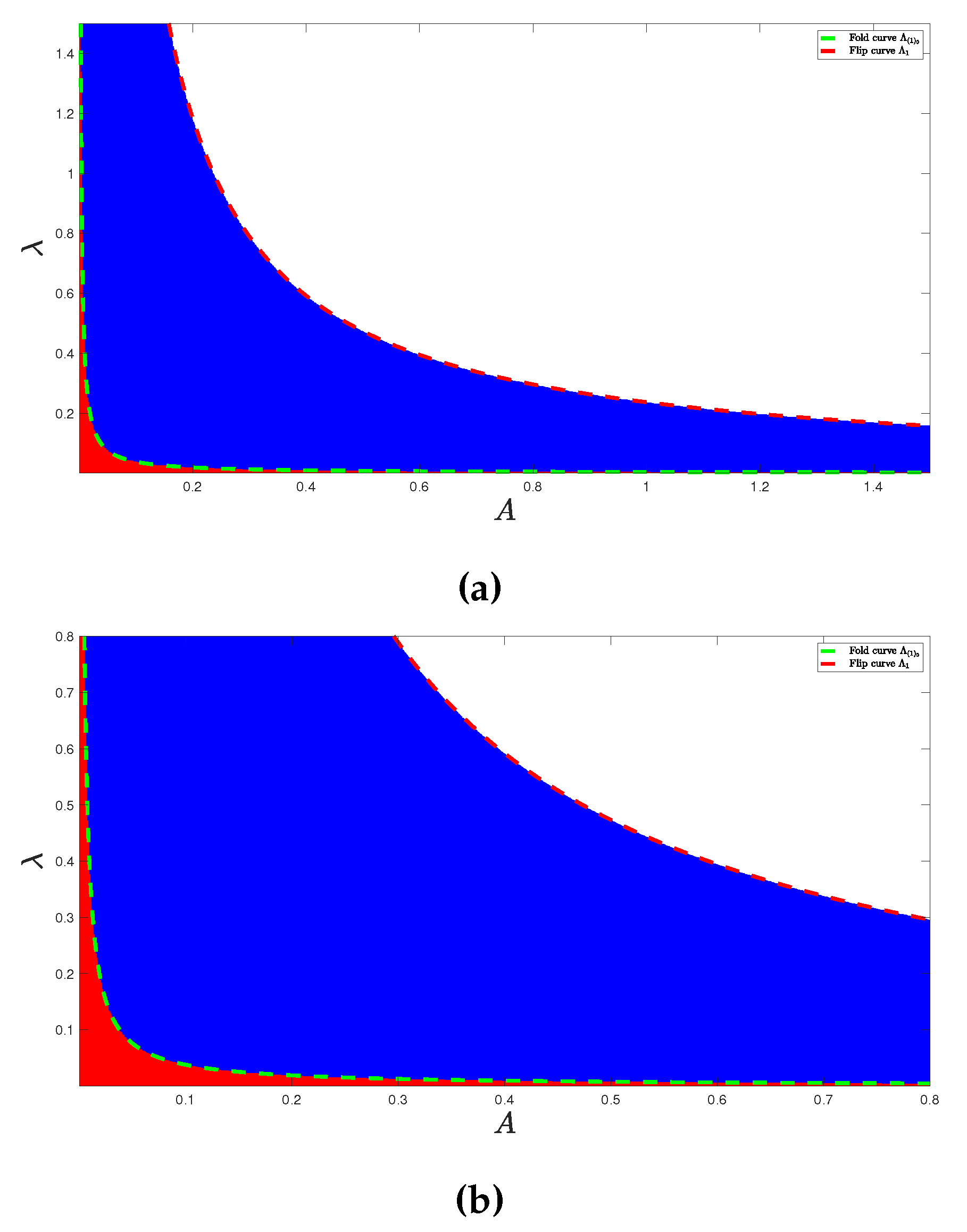
Most real-world control issues focus on both constraint fulfillment and optimality. We want to locate

0.10 \leq u \leq 0.472, 0.5 \leq v \leq min (1, f (u))

with

f (u) = \frac{0.2366}{u}

is the bifurcation curve, for

t \in [0; T]

, as a region included in the stability zone as shown in Figure 11, to minimize

J (u, v)

with

S (0) = S_{0}, I (0) = I_{0}, R (0) = R_{0},

Using minimal control variables

(u, v)

, our goal is to reduce the objective functional specified in (11) by reducing the number of immigrants and sick people. Alternatively, the control variable

(u, v) \in U_{a d}

reflects the proportion of infected and immigrant people that are treated and controlled, respectively, per unit of time, and

U_{a d}

is the control set specified by

U_{a d} = {(u, v) : 0.1 \leq u \leq 0.472, 0.5 \leq v \leq min (1, f (u)), f (u) = \frac{0.2366}{u}} .

7.1. Existence of an Optimal Control

Theorem 6.

There exists control variables

u^{*}

and

v^{*}

so that

J (u^{*}, v^{*}) = min_{(u, v) \in U_{a d}} J (u, v)

Proof.

Drawing upon the seminal works of Fleming and Rishel [15] and Lukes [16], the substantiation of the existence of an optimal control necessitates firstly, the nonemptiness of the controls set and their associated state variables. Secondly, the validation of the convexity and closure properties of the admissible set

U_{a d}

. Lastly, ensuring that the right-hand side of the state system (8) is bounded by a linear function in the state and control variables. □

7.2. Characterization of the Optimal Control

We first describe the Lagrangian for the optimal control issue (8)–(11) before describing the optimal control pair.

L (u, v, I) = \frac{1}{2} u_{t}^{2} + \frac{1}{2} v_{t}^{2} + I_{t}

(12)

and the Hamiltonian H for the control problem by:

H (u, v, I, p_{i}, t) = \frac{1}{2} u_{t}^{2} + \frac{1}{2} v_{t}^{2} + I_{t} + p_{1} (u A - μ S - v λ S I + β R) + p_{2} (v λ S I - (μ + r) I) + p_{3} (r I - (μ + β) R)

(13)

where

p_{i}, i = 1, 2, 3

are the adjoint functions, that the first order necessary conditions for the existence of optimal control are given by the equations

\{\begin{matrix} \frac{\partial H}{\partial u} = 0 \\ \frac{\partial H}{\partial v} = 0 \end{matrix}

(14)

\{\begin{matrix} \frac{d p_{1}}{\partial t} = - \frac{\partial H}{\partial S} \\ \frac{d p_{2}}{\partial t} = - \frac{\partial H}{\partial I} \\ \frac{d p_{3}}{\partial t} = - \frac{\partial H}{\partial R} \end{matrix}

(15)

from (14) we obtain

\{\begin{matrix} \frac{\partial H}{\partial u} = u^{*} + p_{1} A = 0 \\ \frac{\partial H}{\partial v} = v^{*} + (p_{2} - p_{1}) (λ S I) = 0 \end{matrix}

besides, the optimal control pair

(u^{*}, v^{*})

is given by

\{\begin{matrix} u^{*} = min {0.472, max (0.1, - p_{1} A)} \\ v^{*} = min {min (1, f (u^{*})), max (0.5, (p_{1} - p_{2}) (λ S (t) I (t))} \end{matrix}

(16)

after simplified (15) we get

\{\begin{matrix} \frac{d p_{1}}{d t} = p_{1} (μ + v λ I (t)) - p_{2} v λ I (t) \\ \frac{d p_{2}}{d t} = - 1 + p_{1} v λ S (t) - p_{2} v λ S (t) + (μ + r) - p_{3} r \\ \frac{d p_{3}}{d t} = - p_{1} β + p_{3} (μ + β) \end{matrix}

with

p_{1} (T) = p_{2} (T) = p_{3} (T) = 0 .

8. Numerical Simulation

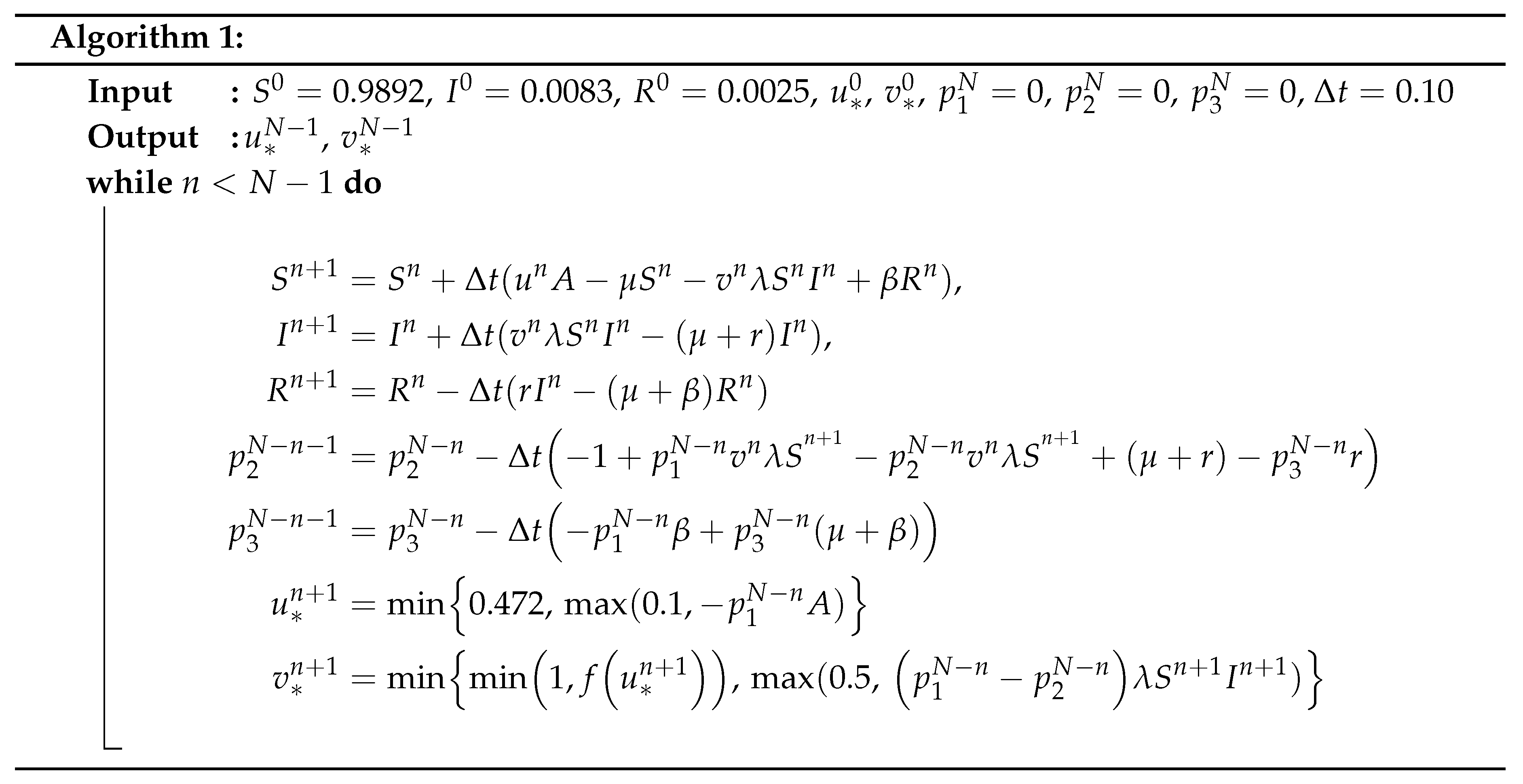
Our primary goal in utilizing the optimal control tool is to minimize the number of infected individuals while maximizing the number of non-infected ones. These objectives are distinctly evident in the numerical outcomes. The following algorithm, which was inspired by Hattaf and Yousfi [17], describes the approximation method for each optimal control. Here, a numerical variant of the forward Euler method with a step size

Δ t

is employed.

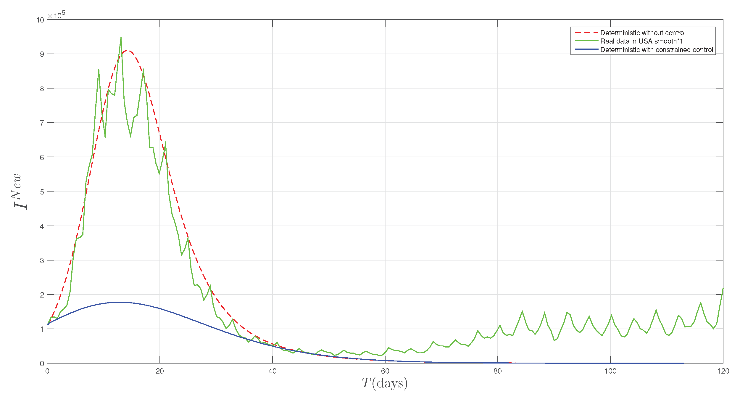
The numerical experimentation performed using Algorithm 1 allow us to affirm the possibility of reducing the density of infected individuals (see Figure 12).

Figure 12 displays the various dynamics of the newly infected population in several aspects. The green color represents the real data in the USA for the wave of COVID-19 between November 06, 2021, and March 10, 2022 3, the red color represents the deterministic dynamic without control and the blue color represents the deterministic dynamic with constrained control. USA could have better controlled the disease by referring to the graph of deterministic with constrained control and this may be due to several factors including the government was not as strict, the people did not respect the gestures of barrier, many people do not respect containment measures and they do not want to get tested to avoid quarantine.

9. Discussion

In this study, we conducted an investigation into the behavior of a discrete SIR epidemic model with loss of immunity. Our analysis revealed the presence of two significant types of bifurcations, flip and transcritical bifurcations, and observe that the parameters

λ

and A have a significant impact on the model’s equilibrium points. As we move forward, it is important to explore additional types of bifurcations, including the Hopf bifurcation. In addition, we introduced a constrained optimal control for a SIRS model that incorporates two control variables, u and v. These variables govern the recruitment rate and infection rate, respectively. The control variable u is used to limit recruitment by controlling border control and regulating the influx of travelers from outside. Meanwhile, the variable v works to minimize infection rates through the implementation of preventive vaccines, adherence to treatment protocols, and adherence to safety and hygiene guidelines, particularly in the context of COVID-19. A novel aspect of our constrained optimal control approach is the introduction of a set of constraints representing the stability zone of cycle 1. We also formulated the objective function for the constrained optimal control problem, enabling us to gain a more comprehensive understanding of epidemic control strategies, To accomplish this work, we constructed the Hamiltonian and applied the Pontryagin’s maximum principle to resolve these problem of constrained optimal control. For the numerical simulation, we use an algorithm, which was inspired by Hattaf and Yousfi [17] founded on the forward and backward difference approximation, Our simulation results indicate that controlling both the recruitment and the infection simultaneously improves the effectiveness of the optimal strategy. It is possible to expand on this work by adding noise and introducing stochastic or partial differential equation.

References

Carcasses, J.P. Determination of different configurations of fold and flip bifurcation curves of a one or two-dimensional map. International Journal of Bifurcation and chaos 1993, 3, 869–902. [Google Scholar] [CrossRef]
Carcasses, J.P. Singularities of the parametric plane of an n-dimensional map. Determination of different configurations of fold and flip bifurcation curves. International Journal of Bifurcation and Chaos 1995, 5, 419–447. [Google Scholar] [CrossRef]
Paeng, S.H.; Lee, J. Continuous and discrete SIR-models with spatial distributions. Journal of Mathematical Biology 2017, 74. [Google Scholar] [CrossRef] [PubMed]
Zhou, L.; Fan, M. Dynamics of an SIR epidemic model with limited medical resources revisited. Nonlinear Analysis: Real World Applications 2012, 13, 312–324. [Google Scholar] [CrossRef]
Muroya, Y.; Enatsu, Y.; Nakata, Y. Monotone iterative techniques to SIRS epidemic models with nonlinear incidence rates and distributed delays. Nonlinear Analysis: Real World Applications 2011, 12, 1897–1910. [Google Scholar] [CrossRef]
Hu, Z.Y.; Teng, Z.; Zhang, L. Stability and bifurcation analysis in a discrete SIR epidemic model. Mathematics and Computers in Simulation 2013. [Google Scholar] [CrossRef]
Eskandari, Z.; Alidousti, J. Stability and codimension 2 bifurcations of a discrete time SIR model. J. Frankl. Inst. 2020, 357, 10937–10959. [Google Scholar] [CrossRef]
Zhang, Z.; Zeb, A.; Hussain, S.; Alzahrani, E. Dynamics of COVID-19 mathematical model with stochastic perturbation. Advances in Difference Equations 2020, 2020. [Google Scholar] [CrossRef] [PubMed]
Pájaro, M.; Fajar, N.M.; Alonso, A.A.; Otero-Muras, I. Stochastic SIR model predicts the evolution of COVID-19 epidemics from public health and wastewater data in small and medium-sized municipalities: A one year study. Chaos, Solitons & Fractals 2022, 164, 112671. [Google Scholar] [CrossRef]
Li, X.; Wang, W. A discrete epidemic model with stage structure. Chaos, Solitons & Fractals 2005, 26, 947–958. [Google Scholar] [CrossRef]
Brauer, F.; Van den Driessche, P.; Wu, J.; Allen, L.J. Mathematical epidemiology; Vol. 1945, Springer, 2008.
Van den Driessche, P. Reproduction numbers of infectious disease models. Infectious disease modelling 2017, 2, 288–303. [Google Scholar] [CrossRef] [PubMed]
Kuznetsov, Y.A.; Kuznetsov, I.A.; Kuznetsov, Y. Elements of applied bifurcation theory; Vol. 112, Springer, 1998.
Mira, C. Chaotic dynamics in two-dimensional noninvertible maps; Vol. 20, World Scientific, 1996.
Fleming, W.H.; Rishel, R.W. Deterministic and stochastic optimal control; Vol. 1, Springer Science & Business Media, 2012.
Lukes, D.L. Differential equations: classical to controlled 1982.
Hattaf, K.; Yousfi, N. Optimal control of a delayed HIV infection model with immune response using an efficient numerical method. International Scholarly Research Notices 2012, 2012. [Google Scholar] [CrossRef]

1	World Bank Open data 2023.
2	World Bank Open data 2023.
3	World Bank Open data 2023.

Figure 1. COVID-19 cases in North America.

Figure 2. Newly infected COVID-19 cases in North America.

Figure 3. COVID-19 cases in North Africa.

Figure 4. Newly infected COVID-19 cases in North Africa.

Figure 5. Transfer diagram for a SIR model with loss of immunity.

Figure 6. Comparison of data values and data model for new infections and new recoveries in Algeria.

Figure 7. Comparison of data values and data model for new infections and new recoveries in USA.

Figure 8. In the

(A, λ)

-parameter plane of model (3) with

μ = 0.0082

r = 0.45314086

h = 0.10

, and

β = 1.16743084

, the two-dimensional bifurcation diagram is depicted. The blue area represents the stability region of the non-zero fixed points (with

k = 1

). The subsequent regions, indicated in yellow (for

k = 2

), cyan (for

k = 4

), and so on, correspond to the period-doubling phenomenon and then it follows the chaotic region.

Figure 8. In the

(A, λ)

-parameter plane of model (3) with

μ = 0.0082

r = 0.45314086

h = 0.10

, and

β = 1.16743084

, the two-dimensional bifurcation diagram is depicted. The blue area represents the stability region of the non-zero fixed points (with

k = 1

). The subsequent regions, indicated in yellow (for

k = 2

), cyan (for

k = 4

), and so on, correspond to the period-doubling phenomenon and then it follows the chaotic region.

Figure 9. Flip bifurcation diagram of model (3) of (a)

S (n)

, (b)

I (n)

and (c)

R (n)

with

λ = 0.86687879, μ = 0.0082, r = 0.45314086, h = 0.10, β = 1.16743084, A \in [0.2, 0.5]

and initial conditions

(S_{0}, I_{0}, R_{0}) = (0.99, 0.01, 0)

Figure 9. Flip bifurcation diagram of model (3) of (a)

S (n)

, (b)

I (n)

and (c)

R (n)

with

λ = 0.86687879, μ = 0.0082, r = 0.45314086, h = 0.10, β = 1.16743084, A \in [0.2, 0.5]

and initial conditions

(S_{0}, I_{0}, R_{0}) = (0.99, 0.01, 0)

Figure 10. Two-dimensional bifurcation diagram of model (3) in

(A, λ)

-parameter plan for

μ = 0.0082, r = 0.45314086, h = 0.10, β = 1.16743084

. The dashed cyan line represents the fold bifurcation curves, outlining the boundaries of stability zones for point

E_{0}

(depicted in blue) and fixed point

E_{1}

(depicted in red).

Figure 10. Two-dimensional bifurcation diagram of model (3) in

(A, λ)

-parameter plan for

μ = 0.0082, r = 0.45314086, h = 0.10, β = 1.16743084

. The dashed cyan line represents the fold bifurcation curves, outlining the boundaries of stability zones for point

E_{0}

(depicted in blue) and fixed point

E_{1}

(depicted in red).

Figure 11. Two-dimensional bifurcation diagram of model (3) in

(A, λ)

-parameter plan for

μ = 0.0082, r = 0.45314086, h = 0.10, β = 1.16743084

. The blue area bounded by the bifurcation curve is the controlling set, in which we study the optimal control included in the stability zone.

Figure 11. Two-dimensional bifurcation diagram of model (3) in

(A, λ)

-parameter plan for

μ = 0.0082, r = 0.45314086, h = 0.10, β = 1.16743084

. The blue area bounded by the bifurcation curve is the controlling set, in which we study the optimal control included in the stability zone.

Figure 12. Dynamic of the newly infected population with constrained control, without control and real data in USA.

Table 1. Values of parameters estimated by optimization.

Parameter	USA	Algeria
$λ$	$0.86687879$	$4.79491051$
$β$	$1.16743084$	$6.27806231$
r	$0.45314086$	$4.36485748$

Disclaimer/Publisher’s Note: The statements, opinions and data contained in all publications are solely those of the individual author(s) and contributor(s) and not of MDPI and/or the editor(s). MDPI and/or the editor(s) disclaim responsibility for any injury to people or property resulting from any ideas, methods, instructions or products referred to in the content.

© 2024 by the authors. Licensee MDPI, Basel, Switzerland. This article is an open access article distributed under the terms and conditions of the Creative Commons Attribution (CC BY) license (http://creativecommons.org/licenses/by/4.0/).

Copyright: This open access article is published under a Creative Commons CC BY 4.0 license, which permit the free download, distribution, and reuse, provided that the author and preprint are cited in any reuse.

MDPI Initiatives

Important Links

Choose an area of interest and we will send you notifications of new preprints at your preferred frequency.

Disclaimer

Analyzing Bifurcations and Optimal Control Strategies in SIRS Epidemic Models: Insights from Theory and COVID-19 Data

Abstract

1. Introduction

2. The Model

3. Data and Parameter Identification (Materials and Methods)

Model Fitting

4. Analysis of Equilibria

5. Bifurcation Analysis

5.1. Bifurcation Curve

5.1.1. Flip Bifurcation

5.1.2. Transcritical Bifurcation

5.2. Numerical Simulation

5.2.1. Flip Bifurcation (or Period Doubling Bifurcation)

5.2.2. Transcritical Bifurcation

6. The Optimal Control Problem

7. SDE with Optimal Control

7.1. Existence of an Optimal Control

7.2. Characterization of the Optimal Control

8. Numerical Simulation

9. Discussion

References

MDPI Initiatives

Important Links

Subscribe