Preprint
Article

Exploitation of Bio Inspired Classifiers for Performance Enhancement in Liver Cirrhosis Detection from Ultrasonic Images

Altmetrics

Downloads

118

Views

53

Comments

0

A peer-reviewed article of this preprint also exists.

This version is not peer-reviewed

Submitted:

10 April 2024

Posted:

10 April 2024

You are already at the latest version

Alerts
Abstract
In the current scenario, liver abnormalities are one of the most serious public health concerns. Cirrhosis of the liver is one of the foremost causes of demise from liver diseases. To accurately predict the status of liver cirrhosis, physicians frequently use automated computer-aided approaches. In this paper the clustering techniques like Fuzzy C Means (FCM), Possibilistic Fuzzy C Means (PFCM), Possibilistic C Means (PCM), Sample Entropy features are extracted from normal and cirrhotic liver ultrasonic Images. The extracted features are classified as normal and Cirrhosis one through Gaussian Mixture Model(GMM), Softmax Dis(SDC), Harmonic Search Algorithm (HSA), SVM(Linear), SVM(RBF), SVM(Polynomial), Artificial Algae Optimization (AAO) and hybrid classifier Artificial Algae Optimization (AAO) with Gaussian Mixture Mode (GMM). The classifiers performances are compared based on Accuracy, F1 Score, MCC, F Measure, Error rate and Jaccard metric (JM).The hybrid classifier AAO GMM with PFCM feature outperforms than other classifiers and attained an accuracy of 99.03 % with MCC of 0.90
Keywords: 
Subject: Engineering  -   Bioengineering

1. Introduction

The improvement of Computer Aided Diagnosis system is essential in the medical field because it can provide an objective and systematic second opinion to the patients [1]. There are various image modalities used for disease diagnosis such as MRI, X ray imaging, Computer Tomography and Ultrasound. Clinicians prefer ultrasound imaging due to its noninvasive, cost-effective, and have no ionizing radiation effects. [2].The sound waves are used to produce internal body structure images such as uterus, liver, blood vessels, kidney instead of radiations. Ultrasound imaging is the effective and safest method to diagnose the abnormalities in abdomen [3]. In humans, the liver is a large and extremely important organ. It is an organ in the body which is involved in metabolism that produces protein, cholesterol, and bile acid among other things. The liver's primary function is to filter blood from the digestive tract before it is distributed to the rest of the body. There are two types of liver diseases: focal(Cyst) and Cirrhosis [4]. Liver cirrhosis is a chronic and progressive liver disease characterized by the irreversible scarring and fibrosis of the liver tissue. It is a consequence of various chronic liver conditions and is often considered the end-stage of liver damage. Liver cirrhosis is a significant global health issue and can lead to severe complications, including liver failure, portal hypertension, and increased risk of liver cancer. Liver cirrhosis often develops gradually, and in the early stages, it may not present noticeable symptoms. However, as the disease progresses, individuals may experience symptoms such as fatigue, weakness, loss of appetite, weight loss, abdominal pain, jaundice (yellowing of the skin and eyes), easy bruising or bleeding, and fluid retention in the abdomen or legs. Among many of the numerous liver disorders that can lead to cirrhosis, some progress quickly while others progress more slowly [5]. Based on data gathered from Cancer Incidence Statistics, Globocan 2020 the estimated prevalence of cirrhosis in the world's population is 4.7% [6]. Hepatic steatosis is the abnormal addition of fat in the liver and hepatic cells [7]. Steatosis can be temporary or permanent that can lead to a variety of problems, including liver cirrhosis. Steatosis is a reversible condition that can be resolved through behavioral changes. Early detection of liver cirrhosis is critical, as there is a chance of saving the liver from serious complications [8]. The abnormality in focal diseases is confined to a small area of liver tissue, whereas in diffused diseases, the abnormality is scattered throughout the liver volume [9]. Liver cancer is a common malignant disease throughout the world, particularly in Southeast Asia and Sub-Saharan Africa. With 500,000 people affected each year, liver cancer is the sixth most common cancer in the world. Globally, the number of people diagnosed with liver cancer is increasing [10]. Every year in India, almost 10 lakh new cases of liver cirrhosis are reported. The World Health Organization ranks liver disease as the tenth leading cause of death in India [11]. It is important to detect the diseases in early stage. In this paper the liver diseases are detected and classified through known clustering methods and Nature inspired classifiers from ultrasonic image database.
Ultrasonic imaging technique is the widely used imaging modality to diagnose the patient disease condition because it is safe and economical. Various techniques are proposed to diagnose the liver disease by the researcher. Nasrul Humaimi Mahmood [12] et al (2012) suggested a method to enhance the liver diseased region using watershed segmentation method. The ultrasound images are preprocessed and the background markers are computed using thresholding operation to clean up the pixels which are not belongs to any object. The segmentation function is modified to get minimum in foreground and background marker location. After this the watershed transform of the segmented function is calculated to highlight the diseased region of liver image.
Nishant Jain [13] et al (2016) presented a method known as Iterative FCM (IFCM) that can be applied to fragment a focal liver lesion from ultrasound images of the liver. The n cluster FCM method results in a distribution of centroids that is not uniform, whereas the IFCM method results in centroids that are evenly distributed. The author compared IFCM accuracy with edge based active contour Chan-Vese (CV) method and Maximum a Posteriori-Markov Random Field (MAP-MRF) method. The proposed model provides the highest accuracy, 99.8%. Bharath [14] et al (2017) et al proposed a method for differentiating the texture feature of fatty liver that is based on the curvelet transform and the SVD. The gradient as well as the curves in the texture can be improved with the help of the curvelet transform. The curvelet decomposed image is used as a source for the extraction of the SVD features. The classification is performed by the cubic SVM classifier. The proposed technique successfully classified liver fat into four classes with an accuracy of 96.9%. Rajendra Acharya [15] et al (2016) proposed curvelet transform and entropy feature to classify the cirrhosis from ultrasonic images. The HOS phase, fuzzy, Reyni, Shannon, Kapoor, vajda and Yager entropy features are extracted from CT coefficients. The probabilistic neural network classifier is used for classification. Probabilistic neural network (PNN) classifier can distinguish between normal, Fatty Liver Disease (FLD), and cirrhosis with 97.33% accuracy using the proposed method. Rajendra Acharya [16] et al (2016) proposed Radon Transform and DCT for extracting the features for normal and fatty liver images. The images are classified using Decision Tree, K-NN, PNN, SVM, Fuzzy Sugeno and Adaboost classifier and attained higher accuracy.
Wang, Q., et al. (2017) [17] proposes a method for liver cirrhosis detection based on texture analysis and ensemble clustering. Texture features are extracted from liver ultrasound images, and K-means clustering and spectral clustering are applied to partition the feature space. The ensemble clustering results are then used for classification. Saranya, K et al (2019) [18] presents a liver cirrhosis diagnosis method using K-means clustering and SVM classification. Features are extracted from liver ultrasound images, and K-means clustering is applied to group the feature vectors. SVM classifier is used for cirrhosis diagnosis based on the clustered features.
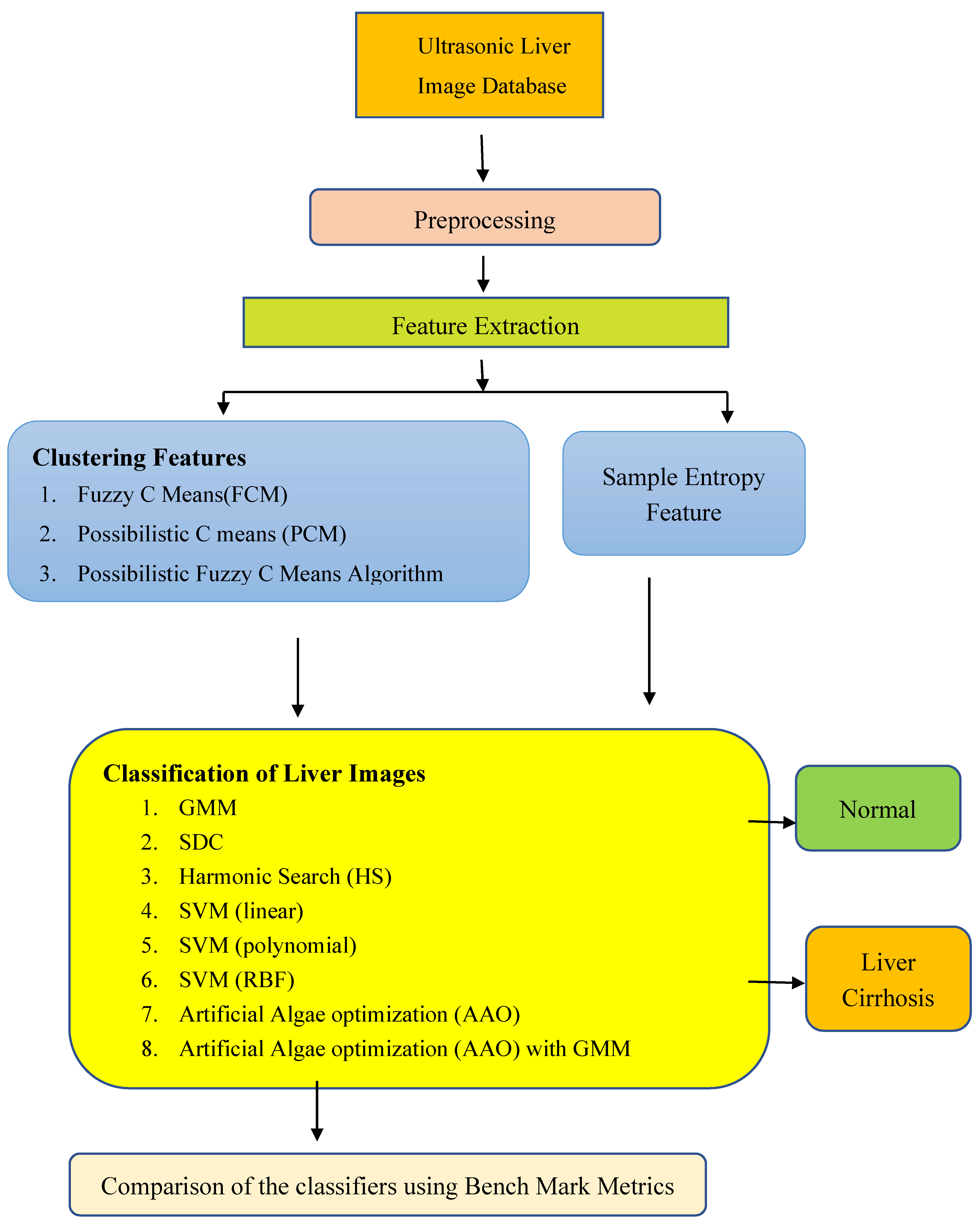
The paper is structured in the following manner. The preprocessing and feature extraction techniques are discussed in section two while the third section deals with the classifiers, namely, GMM, SDC, Harmonic Search, SVM(Linear, Polynomial, RBF), AAO and hybrid classifier AAO with GMM. The results and discussions are explained in the fourth section. The paper is concluded in fifth section.

2. Materials and Methods

In terms of global mortality, cancer is the second-leading cause. When compared to more traditional image processing approaches, ultrasonic imaging seems to be a non-invasive and vital tool for liver cancer identification and categorization. Therefore, ultrasonic imaging technique is used in this study. The primary goal of these studies is to improve liver cancer diagnosis by providing more precise classification systems. Accurately categorizing cancer data helps patients get the care they need at a lower cost, and also reduces their own risk of developing the disease. There is a tendency for the classifier accuracy to decrease due to the presence of unimportant and noisy images in the captured image. The effective filtering method is used for remove the unwanted signal in ultrasonic images
The overall schematic representation for detecting Liver Cirrhosis from ultrasound images is shown in Figure 1 and detailed workflow will be illustrated in Figure 2. This article explores at a group of 1859 ultrasound images from the Cancer Imaging Archive (929 normal, 930 abnormal). Each picture measures around 790 by 960 pixels. Wessner, C., A. Lyshchik, and J. Eisenbrey (2021). URL: https://doi.org/10.7937/TCIA.2021.v4z7-tc39. The images are preprocessed before feature extraction. The clustering based features such as FCM, PCM, FPCM and sample entropy features are extracted and given as input to the classifiers .Totally eight classifiers are employed in this work. The MATLAB 2014a software is used to carry out this investigation [19]. The performance of classifiers is evaluated and discriminated using parameter metrics for clustered based features and sample entropy feature.

2.1. Preprocessing

Speckle noise is the main thing that changes usefulness of the ultrasonic images. The speckle noise affects the contrast and resolution of the images. So effective noise filtering technique will be utilized for elimination of noise, the adaptive wiener filter is used in this work to suppress the noise [20]. In adaptive wiener filtering, the filter’s output is modified based on the image’s local variation. The final objective is to achieve the smallest possible mean square difference among the restored and original images. This method is superior to other filters in terms of filtering effect, and it is especially helpful for conserving the image’s edges and high-frequency regions [21]. The below equation represents the speckle noise model
g ( q , r ) = h ( q , r ) + m ( q , r )
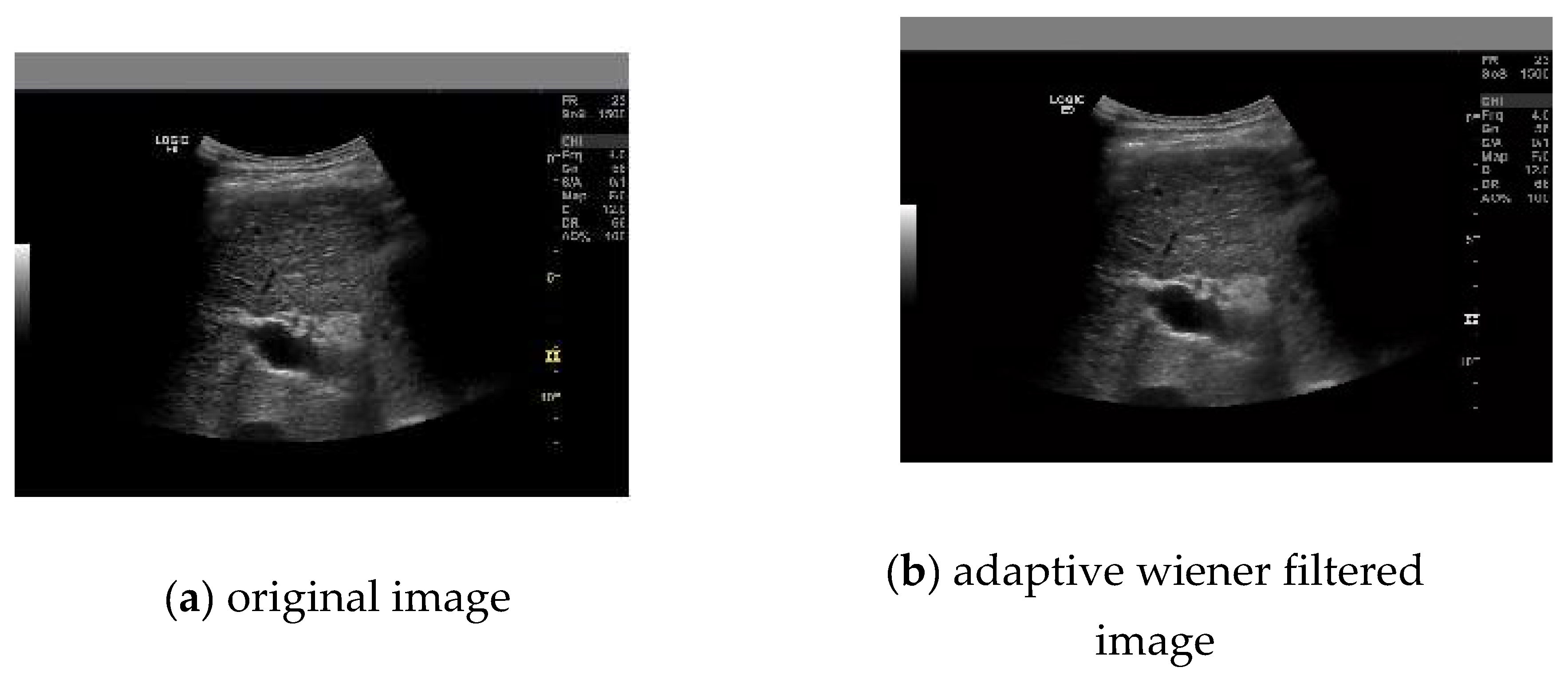
where g(q,r) represents the noisy image , the noise image is denoted as h(q,r) and the noise signal is m(q,r)[18]. In adaptive wiener filtering, the filter’s final result is adjusted according to the image’s local variation. To some extent, the adaptive filter can fine-tune itself. Automatically adjusting to different input signals, it improves image restoration quality by minimizing the mean square error. When compared to other filters, this one has a better filtering effect, and it works great for keeping the image’s edges and high-frequency areas intact. The below Figure 3 shows the original and filtered ultrasonic images.

2.2. Clustering Methods for Feature Extraction

The function of feature extraction is to convert raw data input into numerical features. Typically, images are represented as raw data. Its purpose is to extract characteristics that indicate the meaningful information extraction from Ultrasonic Images. The preprocessed and noise removed ultrasound images are further processed to extract the features by employing three clustering algorithms and one entropy feature and the features are Possibilistic Fuzzy C Means (PFCM), Fuzzy C Means Clustering (FCM) , Possibilistic C means (PCM) techniques and Sample Entropy. In order to expedite the embedded distinct properties of the liver image among the classes are analyzed from the statistical variables like Mean, Variance, Skewness, Kurtosis, and Pearson Correlation Coefficient (PCC) as shown in Table 1.
As observed from the Table 1 that for PCM features exhibits poor values of mean and variance among the classes and Skewness represents one sided in nature along with tailed kurtosis. The intra class PCC is identified with no correlation. The CCA represents higher correlation across the classes for all the feature extraction methods. As in the case of FCM method only PCC indicates slight improvement in the intra class correlation. For PFCM features demonstrates positive Skewness and tailed kurtosis with moderate PCC for intra classes. The sample entropy features depicts negative Skewness and flat kurtosis with improved PCC for intra classes. From the statistical parameters of the extracted features through four different methods as shown in the Table 1 clearly demonstrates the properties of non-Gaussian, less correlation, overlapping and skewed nature of the features.

2.2.1. Fuzzy C Means Clustering (FCM)

One of the most basic methods of fuzzy clustering is Fuzzy C-Means (FCM). This process of adaptation converges to a stationary state, or local minimum. The FCM method is used to examine data sets that are connected through both Euclidean and non-Euclidean distances [22]. In FCM the data point may be a member of multiple clusters simultaneously and it is known as membership function. Based on the similarity the membership value is assigned to a data sample and normally the value lies between 0 to 1. The optimum solution is obtained by continuously updating the cluster center and membership function. The updated values are obtained by solving cost function [23].
Let Y={y1,y2,y3,…,yN}where N represents the data sample. It is divided into ‘c’ clusters by reducing the cost function.
K = l = 1 M m = 1 c w l m   n y l u m 2
For mth cluster wlm represents the membership of yl. The mth cluster is represented by um and . represents norm metric [24].

2.2.2. Possibilistic C means (PCM) Algorithm

PCM is another clustering technique developed by keller in 1997.This approach is suitable for unwinding compact clusters [25].The approach is distinguished from previous clustering algorithms in that the resultant subdivision of the data can be considered as a probabilistic partition and the membership values as degrees of possibility of the points belonging to the classes. A scalar vij can be used to associate each data vector yi with a cluster Cj.[26]
Consider an unnamed dataset Y={y1,y2,y3,…,yn} P r . The objective function is minimized to determine the partitioning of Y into 1<c<m fuzzy subsets.
K m ( E , F ) = a = 1 c b = 1 m v a b   n F a b   2 + a = 1 c b = 1 m ( 1 v a b ) m
Here Fab= y b v a , 0 v a b 1 and the number of clusters are given as “c”, the number of data points is denoted as m, The positive constant η a is given by
η a = β a = 1 n v a b   m F a b   2 b = 1 n v a b   m , β > 0
The value of η a is always 1for all values of a,b. F a , b = y a v b > 0 . M i n ( E , F ) K m ( E , F ) is improved and the following PCM method is derived.[30]
v a b = 1 + F a b   2 η a 1 m 1 1 , a , b

2.2.3. Possibilistic Fuzzy C Means Algorithm (PFCM)

Outliers and noise are two of FCM's greatest issues. To address this issue, the PCM algorithm is offered, however, it is sensitive to initial conditions and suffers from coincident clustering. As a hybrid of FCM and PCM, PFCM is introduced [27].In noisy data, it is suggested that both hard and soft clustering use a norm parameter other than the Euclidean norm in order to improve FCM performance. The FCM algorithm finds the most compact clusters by diminishing the loss function.[28]
J ( X , Y , Z ; A ) = k = 1 M l = 1 c ( C F C M x k l   η + C P C M y k l   η ) a k z l 2 + l = 1 c γ l + k = 1 m ( 1 Z k l ) η
Here C F C M 0 & C P C M 0 are the respective significance of the membership class x k l , Z k l

2.2.4. Sample Entropy as a Feature

Entropy is a term that deals with prediction and uncertainty, with higher entropy levels always indicating a lack of system order and an increase in randomness. Sample Entropy-based feature extraction provides a valuable tool for quantifying the complexity and regularity of signals. It offers a means to extract informative features that capture important characteristics of the underlying dynamics. These features can be used for various analysis tasks, including classification, anomaly detection, and monitoring in different domains. Sample Entropy is fewer susceptible to noise and can be used with short time series data. The negative logarithm of the conditional probability that two sequences identical for m points persist like at the next point is SampEnt(m,r,N). A maximum level usually indicates more irregularity or complexity in the data set.[29]
S a m p E n t ( n , p ) = L i m M ln C m ( p ) D m ( p )
For finite number of data points the sample entropy is given as follows
S a m p E n t p , r , N = ln D m ( r ) C m ( r )
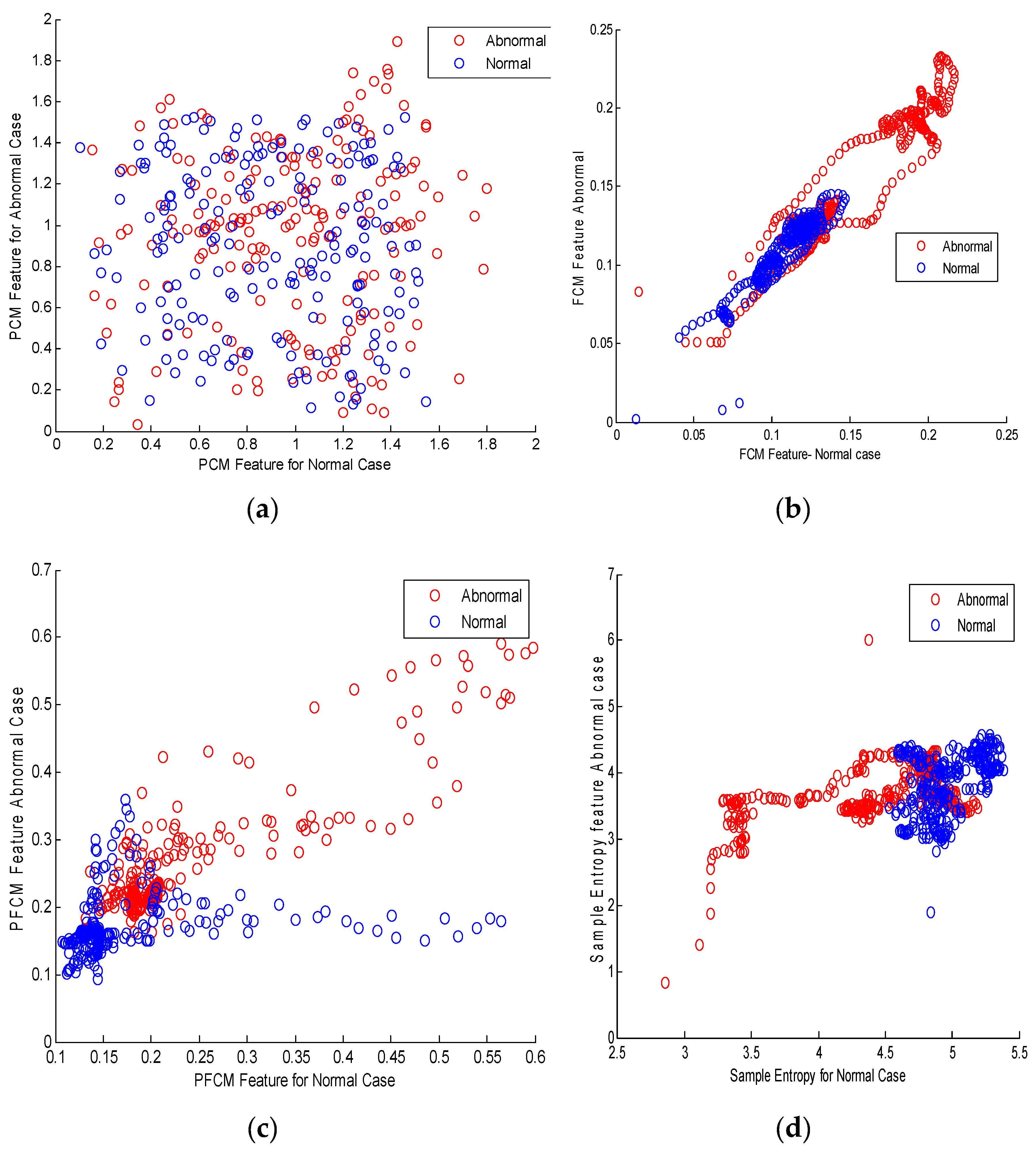
Figure 4a illustrate the scatter plot for normal and cirrhosis cases for PCM feature. It clearly indicates the features are fully scattered with outliers. Figure 4b shows the scatter plot for FCM features which indicates the overlapped and nonlinear properties of the feature. The scattered plot for PFCM feature is depicted in Figure 4c. It indicates the normal and cirrhosis features are overlapped with outlier and partially scattered. From scatter plot of PFCM feature it is observed like a traditional XOR problem. Figure 4d shows scatter plot for sample entropy feature. This indicates that the features are nonlinear, overlapped and non-Gaussian.

3. Bio Inspired Classifiers for Classification of Liver Cirrhosis from Extracted Features

The various bio inspired classifiers are explored in this article for classification of Liver abnormality as explained below.

3.1. Gaussian Mixture Model (GMM) as a Classifier

A Gaussian Mixture Model (GMM) is a type of prediction model in which all data samples are formed from a combination of finite Gaussian densities [30]. Gaussian Mixture Model (GMM) is a probabilistic model that represents a probability distribution as a weighted sum of multiple Gaussian distributions. Each Gaussian component in the mixture model represents a cluster or a mode in the underlying data distribution. GMMs have been widely used for various tasks, including clustering, density estimation, and data modeling. As a result, GMM uses a series of Gaussian densities to model the distribution of a data collection. Consider a n dimensional sample space with random vector y and it obeys the Gaussian distribution, then PDF is given as [31]
P ( y ) = 1 ( 2 π ) m / 2 1 / 2 e ( 1 / 2 ) ( y μ ) T 1 ( y μ )
where μ denotes the mean, covariance matric is . The two parameters μ , define the Gaussian distribution.

3.2. Softmax Discriminant Classifier (SDC)

Softmax discriminant classifier's objective is to accurately identify the class to which a test sample fits. It is accomplished by calculating the distance between both the training sample and the test sample of that particular class. Assume the training set K = K 1 , K 2 , ... , K m a × b derives from ‘m’ different classes, K m = [ K 1 m , K 2 m , ... , K b m m ] a × b m denotes the ‘bm’ samples from mth class where j = 1 m b j = b [32]. We use the m class samples to find the test sample with the least amount of reconstruction error. The concept of SDC can be accomplished by increasing the value of non-linear conversion among the q class sample and the test sample. The SDC is given by
g ( k ) = arg max j Z k j
g ( k ) = arg max j log i = 1 d i exp ( λ k k i j 2 )
The distance between j th class and test sample is denoted by g(k). λ should be greater than zero to need to give penalty cost. Hence if K detects to the j th class then k and k i j would have same characteristic and k k i j 2 is progressing class towards zero and the maximum possible value is achieved by maximizing Z j k in an asymptotic manner. [33]

3.3. Harmonic Search Algorithm (HSA) as a Classifier

HSA is an evolutionary algorithm which is inspired by musicians' improvising. This algorithm (HS) aims to mimic improvisational procedure used by musicians while presenting music. In the traditional way of improvising, to make wonderful music, musicians constantly fine-tune their instruments [34]. The fundamental stages of HS execution are as follows.
1. Parameters for the HS algorithm and problem configuration:
Here the objective function f(k) is subject to k i K , i = 1 , 2 , 3 , ... , M is minimized or maximized using optimization technique. A set of decision variable is represented by M, then for each variable the set of all possible variables are represented by K i.e k i L K k i v . The upper and lower boundries for each decision variable is denoted by kiL & kiv. To initialize the HS algorithm the following parameters are considered.
  • Harmony Memory size (SHM)
  • Harmony memory consideration rate (HMCR)
  • Pitch Adjusting rate(PAR)
  • Bandwidh(BW)
  • Maximum number of Iteration(Maxitr)
2. Initialization of Harmony Memory:
In the form of a matrix, all of the decision variables are saved in the memory of the system. The initial HM for the globally optimal solution is drawn from a uniformly distributed distribution of values within kiL and kiv.
3. New Harmony Development:
The following limitations are used to create a new harmony through the solution development phase.
  • Consideration of memory
  • Pitch change
  • Random selection
4. Harmony memory Updation:
Find the harmony vector fitness function. The New Harmony vector should replace the old one if its fitness function is relatively low. Otherwise, keep the old harmony vector.
5. Evaluate the ending criteria:
Repeat step 3 & 4 followed until maximum number of iteration achieved.
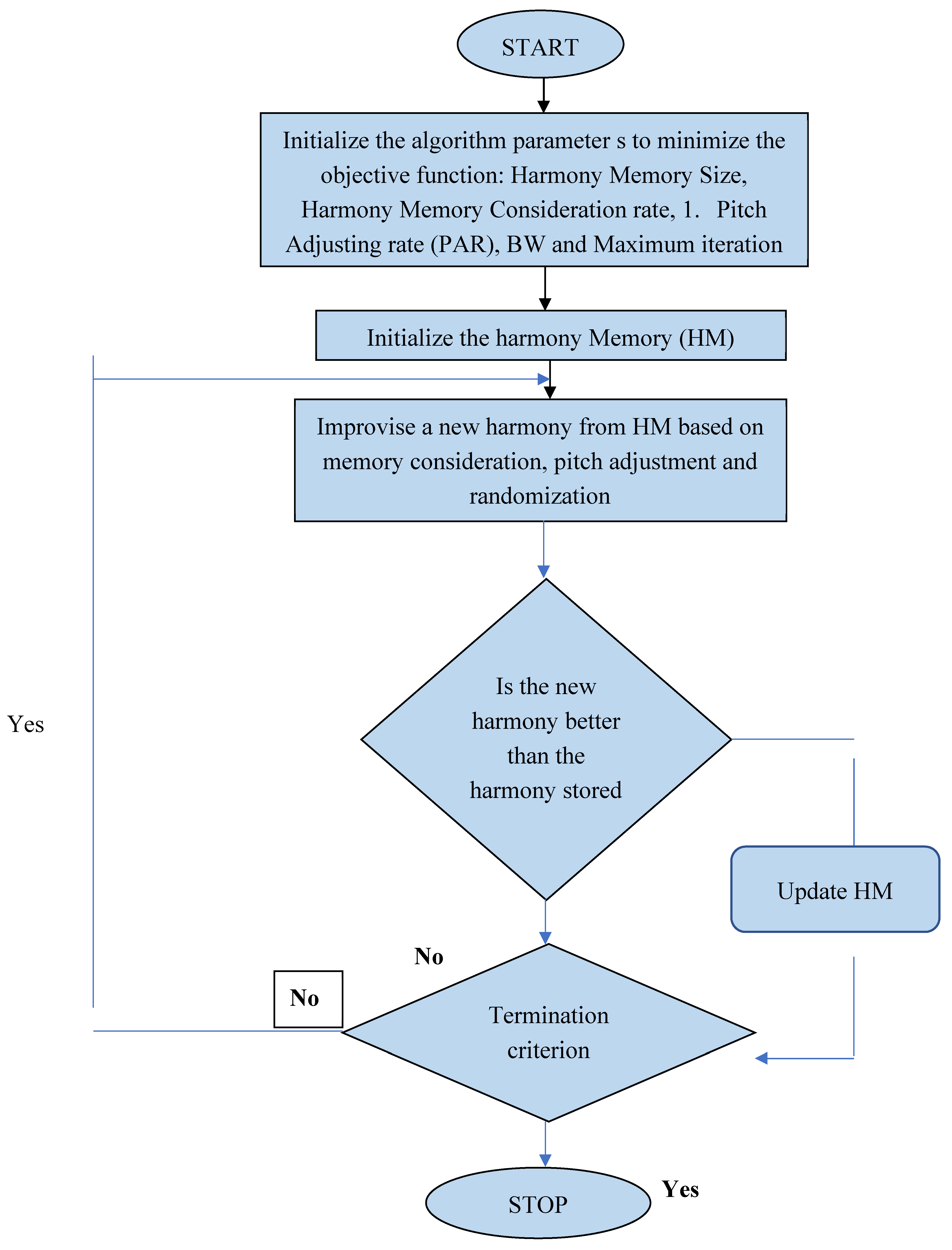
Figure 5 shows the cirrhosis classification. HS-based cirrhosis classification uses ultrasound liver images one by one. The clustered based features are extracted. The normalized n mean feature is set as HM for classification. i.e the harmony memory size is ‘n’, after this initialization harmonic search is started. The class as a whole will reach a state of perfect harmony when maximum number of iterations is done. However, in the case of binary classification exact harmony is not needed, thus the highest number of iteration is picked as the stopping condition [35].
On the basis of learning by doing, the value of SHM was decided to be 16, and the matrix was set to 3. The limits of the decision variables kiL is 1 and kiv is 0.1. The BW and variation in pitch-control amount is selected as 0.1. The final stage of liver cirrhosis classification is depicted in Figure 5. The best harmony vector is taken as the result of the harmony search for each image, and the mean of the best harmony vector is then determined.

3.4. Support Vector Machine as a Classifier

One of the most powerful supervised learning algorithms is SVM. It is a binary classifier and a statistical learning method. For image classification, SVM is incredibly intelligent. It's utilized in hyper plane to set decision boundaries as well as separate relevant and irrelevant vectors and sort data points into different classifications [36].In SVM, input data is transferred into higher dimensional feature space using kernel functions for multiclass problems. The direct acyclic graph, binary tree , one against one and one against all, these are some techniques to solve multi class SVM problem. Consider a feature ‘Z’ with label ‘h’ for a binary classifier, the class labels are represented as h ( 1 , 1 ) . Assume the parameters y,a instead of the classifier with vector θ , the classifier equation is given as
g y , a ( z ) = K ( y T z + a )
Here k(x) =1 if x 0 and k(x)=-1 otherwise. The term ‘a’ is separated from other parameters using y,a. In this work we used SVM with three kernel (Radial Basis function (RBF), linear, Polynomial). [37]
1. SVM with RBF (Radial Basis function) Kernel:
H ( y i , y j ) = exp ( γ y i y j 2 2 σ 2
2. SVM with Linear Kernel:
H ( y i y j   ) = y i T y j
3. SVM with Polynomial Kernel with degree d:
H ( y i y j   ) = ( y i T y j + 1 ) j   d

3.5. Artificial Algae Optimization Algorithm (AAO)

In 2015, AAO was introduced as a population-based optimization technique. Algal Colony Optimization (AAO) is an attempt to model biological behavior in algae colonies in order to find efficient solutions to optimization problems with a repeatedly solution space [38]. A colony of algae is a collection of algal cells that live together. For example, when a single algal cell divides into two, both of the resulting cells continue to reside in close proximity to one another. An algal colony works similar a single cell, changes in a clump, and cells in the colony may die if living conditions are inappropriate. An external force, such as shear, or other unfavorable conditions, may disperse the colony, with each dispersed section becoming a new colony as life progresses.
P o p u l a t i o n A lg a l c o l o n y = y 1 1 y 1 2 . . y 1 C y 2 1 . . y 2 2 . . . . y 2 C . . y N 1 y N 2 . . y N C
where y j i is algal cell in i th element of j th algal colony. The evolutionary process, helical movement, and adaptability are the three phases of AAO.[39]
Evolutionary Process:
The growth characteristics of the algae are defined by evolutionary process. It can be modeled using Monod equation
H j t + 1 = e i ( y ) L + e i ( y ) H i t , ( i = 1 , 2 , 3... , N )
The size of the algal colony is H1and the number of algal colony is represented by ‘N’.[40]
Adaptation Process:
An undeveloped algal colony will go through the process of adaptation in an effort to model itself after the most dominant algal colony in its surrounding atmosphere. This procedure is completed when the algorithm's hunger level is changed. For every artificial algae, the initial starving value is zero. When algae are subjected to insufficient illumination, the starvation value increases as ‘t’ grows.[41]
S t a r v i n g t = M a x B j T , ( j = 1 , 2 , 3 , ... N )
Straving   t + 1 = S t a r v i n g t + ( b i g g e s t t S t a r v i n g t ) r a n d
Helical Movement
To maximize their exposure to light, algal cells and colonies migrate to and reside near the water's surface. Real-life algal cells move helical. Shear force (viscous drag) is proportional to algal cell size and gravity is zero in AAA. Its model volume decides its size. As an effect, the hemisphere's surface area is converted to friction surface.
T y j = 2 π 3 H j π 3 2
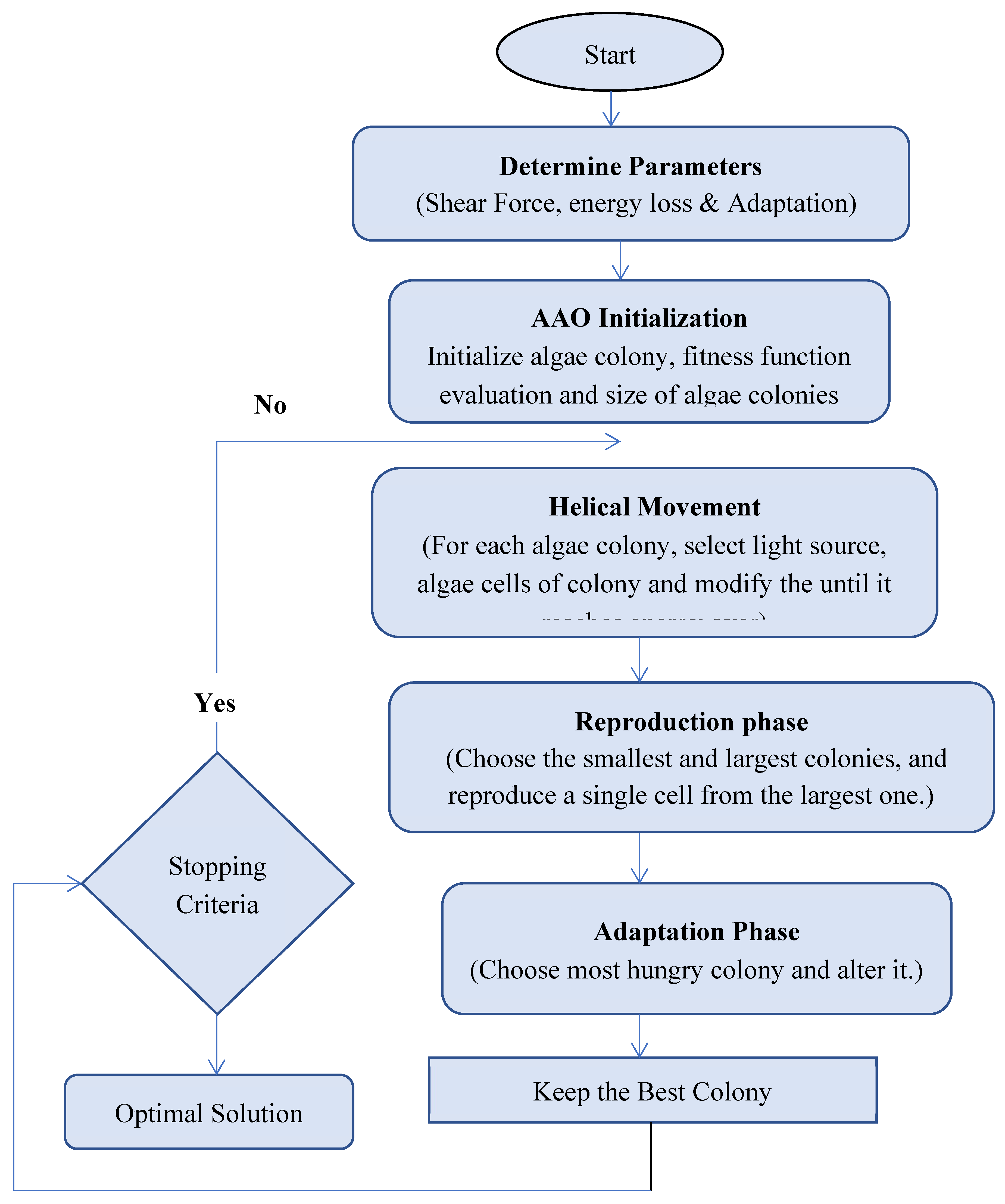
The helical motion of an algal cell is based on a random process that occurs in all three planes. [42] Figure 6 depicts the parameter selection for AAO algorithm for classification of liver cirrhosis.

3.6. AAO with GMM

The combination of AAO and GMM as a classifier leverages the optimization capabilities of AAO to explore and exploit the search space effectively. GMM, as a classifier, provides a probabilistic framework for modeling and classifying the data based on the extracted features. This hybrid approach aims to improve the performance of classification tasks by incorporating the strengths of both AAO and GMM. The proposed method combines AAO with GMM to get the optimum result. It is observed that in Table 2 compared with harmonic search algorithm the AAO attain minimum Mean Square Error (MSE). Hence the AAO is hybridizing with GMM.

4. Results and Discussion

The classifier's efficiency is measured using a ten-fold cross-validation procedure, and the measures employed in this work are as follows: If a positive sample is correctly predicted as positive, it is referred to as (TP) True Positive. If a negative sample is correctly predicted as negative, it is said to be (TN) True Negative. A false positive (FP) occurs when a result is incorrectly assumed to be positive when it is actually negative. A false negative (FN) happens when a result is mistakenly assumed to be negative but is really positive.
The Mean Square Error can be calculated using the below formula
M S E = 1 K j = 1 K ( O j T i ) 2
where Oj is the computed value at a particular time and Ti is the desired value at system i. The training was carried out in such a way that a method through which the classifier's MSE is reduced to a very small value. Tables 2 compare the MSE of eight classifiers with three set of clustering based features and one entropy based feature for classification of normal and cirrhosis liver images.
From Table 2 it is observed that for PCM feature AAO, AAO with GMM, SVM (RBF) classifier provide minimum MSE value of 2.31E-05, 2.22E-05, 2.53E-05 respectively and at the same time SVM (RBF), AAO classifier leads to Type-I (False Positive) error. The classifiers GMM,SDC,HS, SVM(linear),SVM(polynomial) leads to both Type-I, Type-II error(False Negative) and got maximum MSE values of 1.09E-04, 5.19E-05,1.17E-04, 3.33E-04, 7.38E-05 respectively. Similarly for FCM feature the AAO algorithm provide least MSE of 1.22E-06 .The classifiers HS, SVM (Linear) leads to Type-I error and GMM leads to type-II error. As a whole the lower error 1.22E-05, 4.57E-06, 1.39E-06 obtained for SVM(Polynomial), SVM(RBF), AAO with GMM classifiers and Maximum MSE obtained for GMM,SDC,HS, SVM (Linear) and the values are 1.37E-05, 5.78E-05, 2.40E-05, 3.42E-04 .For PFCM feature again AAO with GMM hybrid classifier yields Minimum MSE of 2.6E-07 and HS bring out Type-I error, SDC leads to Type II error. So the classifiers SDC, HS,SVM(linear) results maximum MSE of 3.701E-05, 1.249E-05, 1.306E-05 and GMM,SVM(Polynomial),SVM(RBF), AAO bring about lower MSE values of 2.05E-06, 8.545E-06, 3.145E-06, 5.125E-06 respectively. Likely for Sample entropy feature minimum MSE of 8.1E-07attained for AAO classifier. The GMM, SVM polynomial Classifiers leads to Type I and Type II error. The lower MSE values of 1.265E-05, 1.945E-06, and 2.745E-06 attained for SDC, SVM (RBF), and AAO with GMM classifier. But the classifiers GMM, HS, SVM (linear), SVM (Polynomial) achieved a maximal MSE of 1.331E-05, 4.42E-05, 5.545E-05, 1.702E-05 correspondingly.

4.1. Selection of Classifier Parameters

The ultrasonic liver dataset consisted of two distinct classes, specifically cirrhosis and normal, which were used to determine the target values. The target variable was accurately chosen to contain greater values within the range of 0 to 1. The following criterion is applied in order to select the target for the Normal case T Nor
1 K i = 1 K μ i T N o r m
For K number of normal images the mean for normalized features are represented by μ i and the value is between 0-1. Abnormal case the condition for target selection is
1 K j = 1 K μ j T A b n n o r m a l
Here μ j represents the mean of normalized features for abnormal case. For best Classification T A b n o r m a l T N o r m 0.5 .Considering the above-mentioned statement, the target for this work has been set at 0.1 and 0.85 for normal and Abnormal, correspondingly.
Table 3 shows the trial and error method for selecting the best parameters for the classifier during the training process. For controlling the convergence criteria, the maximum iteration is set to 1000.

4.2. Classifier Performance Analysis

The following parameters are considered to assess the performance of the classifiers. The parameters are Accuracy, F1Score, Mathew Correlation Coefficient (MCC), F Measure (FM), Error Rate(ER), Jaccard metric (JM). Below is a formula that can be used to determine the overall efficiency of the classification method:
A c c u r a c y ( A ) = T P + T N T P + T N + F P + F N 100
F 1 S c o r e = 2 T P 2 T P + F P + F N 100
Mathew   Correlation   Coefficient M C C = T P T N ( F P F N ) ( T P + F P ) ( T P + F N ) ( T N + F P ) ( T N + F N ) 100
F M e a s u r e = T P T P + F P T P T P + F N
E r r o r R a t e ( E R ) = F N + T P T N + T P + F N + F P 100
J a c c a r d M e t r i c ( J M ) = T P T P + F P + F N 100
The performance analysis of the classifiers is exhibited in Table 4 for three clustered based feature and sample entropy feature. As observed from Table 4 the PFCM clustering features with the hybrid classifier AAO-GMM reached a prominent high level in all bench mark parameters such as accuracy of 99.03%, F1 score of 95.24% , MCC with 0.90, FM of 0.95 and achieved a lower error rate of 0.97% with Jaccard metric of 90.91%. Based on the result we can now declare the hybrid classifier AAO with GMM to be outperforming classifier for PFCM feature. Simultaneously from Table 4 it is observed that SVM(Linear) classifier attained lower level performance in terms of accuracy of 52.38%, F1 score of 53.49% and lower MCC value of 0.05, FM is 0.43 and higher error rate of 47.62% with JM of 36.51%. Based on the performance the SVM classifier is least performing classifier in the detection of liver disease detection. By analysing individual feature analysis, for PCM feature the hybrid classifier AAO with GMM perform better than other classifiers based on the parameter FM of 0.79 and Jaccard Metric of 64.29%.The SVM (Linear) is the lower performing classifiers because of higher error rate of 47.62% with reduced MCC of 0.05. Similarly for FCM feature the heuristic classifier AAO attained a best accuracy of 91.67% with good MCC agreement of 0.83 and lower error rate of 8.33%. At the same time for PFCM feature the hybrid classifier AAO with GMM attained a higher accuracy of 99.03 % because of lower error rate of 0.97%. At the same way the AAO classifier for sample entropy feature achieve a good accuracy of 94.05%, F1 score of 94.12%with good MCC value of 0.88 and this is reduced to lower error rate which is 5.95%. It is also perceived from Table 4 while we add AAO with GMM together in cascade form the performance of the classifier is increased in terms of accuracy, F1 score, MCC,FM, JM with lower error rate.
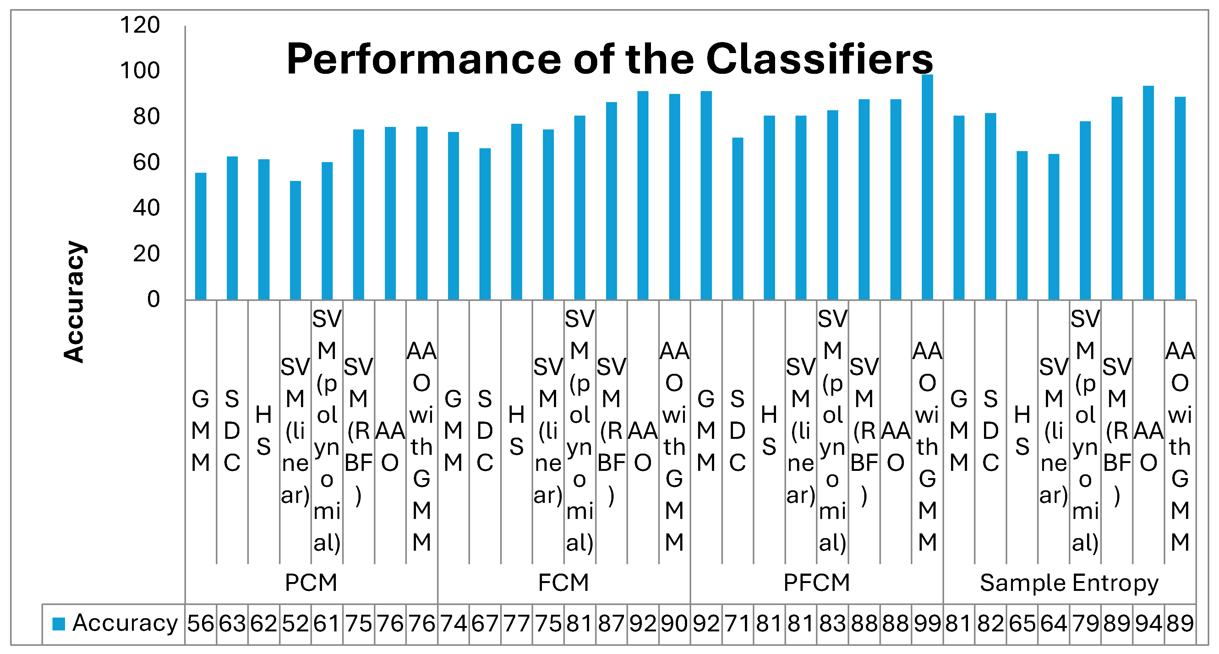
Figure 7 depicts the performance indicators Comparing Accuracy of classifiers for PCM, FCM, PFCM and sample entropy features for different classifiers.
Table 5 shows the consolidated classifier performance for all the classifiers with four different feature extraction techniques. The hybrid classifier AAO –GMM is the best performing classifier for PCM feature with an accuracy of 76.19% and SVM - linear classifier is the least performing classifier for PCM feature with an accuracy of 52.38% with minimum JM of 36.51%. For PCM feature the bio inspired classifier AAO gives good accuracy of 91.67% with 91.76 % of F1 score and the lower accuracy obtained for SDC classifier with a value of 6.67%. Next again the Hybrid classifier AAO-GMM attained a very high accuracy of 99.03% for PFCM feature with a good F1 score of 95.24%. At the same time the SDC classifier attained lowest accuracy of 71.43%. For sample entropy feature the bio inspired classifier AAO attained a good accuracy of 94.05 % and lowest of 64.29% for SVM linear classifier. While comparing all the classifiers with four feature extraction technique the hybrid classifiers are performing better and provide maximum accuracy due to the hybrid nature of GMM and bio inspired classifier. Among the eight classifiers the SVM linear and SDC classifiers are least performing classifier due to the nonlinear nature and the presence of outlier in the extracted features.
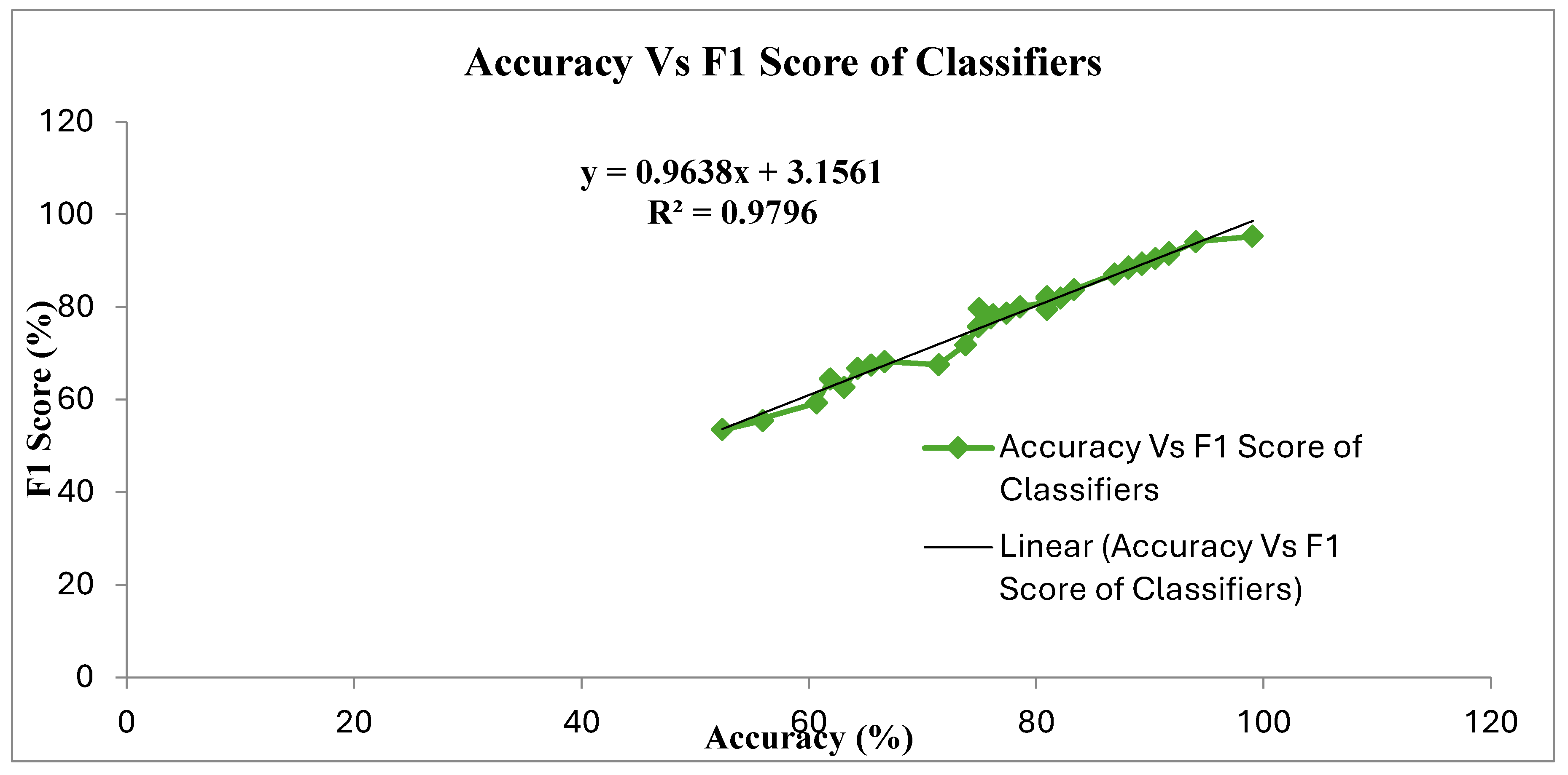
Figure 8 shows the overall accuracy and F1 score analysis of the classifiers with the four feature extraction technique. The linear nature of the classifiers is exhibited below 65% and above 85% accuracy in Figure 8. In the range between 65% to 85%, the classifiers exhibit nonlinearity.

5. Conclusions

The foremost aim of this work is to classify the ultrasonic liver images as normal or cirrhosis in an accurate manner. The features of ultrasonic images are extracted using PCM, FCM, PFCM, sample entropy methods. There are eight classifiers such as GMM, SDC, Harmonic search, AAO, SVM-Linear, SVM-Polynomial, SVM-RBF, AAO and hybrid classifier AAO-GMM are employed for classification purpose .In that the hybrid classifier AAO-GMM for PFCM feature attained a better accuracy of 99.03% followed by sample entropy based feature with AAO classifier with an accuracy of 94.04%. Further research will be the direction of analyzing Deep learning features with CNN, DNN and LSTM architectures for the of liver abnormalities with multiple databases.

References

  1. S. K. Randhawa, R. K. Sunkaria and A. K. Bedi, "Prediction of Liver Cirrhosis Using Weighted Fisher Discriminant Ratio Algorithm," 2018 First International Conference on Secure Cyber Computing and Communication (ICSCCC), 2018, pp. 184-187. [CrossRef]
  2. R.Karthikamani,Harikumar Rajaguru Analysis Of K Means Clustering And Classifiers In Diagnosing Abnormality Of The Ultrasonic Liver Images International Journal of Aquatic Science ISSN: 2008-8019,Vol 12, Issue 03, 2021pp1589-1595.
  3. Web reference, https://www.mana.md/different-uses-for-ultrasound/.
  4. Jagdeep Singh, SachinBagga, RanjodhKaur, Software-based Prediction of Liver Disease with Feature Selection and Classification Techniques, Procedia Computer Science,Volume 167,2020,Pages 1970-1980,ISSN 1877-0509.
  5. M. Tsiplakidou, M. G. Tsipouras, P. Manousou, N. Giannakeas and A. T. Tzallas, "Automated Hepatic Steatosis Assessment through Liver Biopsy Image Processing," 2016 IEEE 18th Conference on Business Informatics (CBI), 2016, pp. 61-67. [CrossRef]
  6. https://gco.iarc.fr/today/data/factsheets/cancers/39-All-cancers-fact-sheet.pdf.
  7. R. Karthikamani; Harikumar Rajaguru, Detection of Liver Cirrhosis in Ultrasonic Images from GLCM Features and Classifiers, S. Vlad and N. M. Roman(Eds.): MEDITECH 2020, IFMBE Proceedings 88, Springer, pp. 161–172, 2022. [Google Scholar] [CrossRef]
  8. 8. Harikumar Rajaguru, R.Karthikamani, Detection Of Abnormal Liver In Ultrasonic Images From FCM Features International Journal of Aquatic Science ISSN: 2008-8019,Vol 12, Issue 03,2021pp1581-1588.
  9. R. Suganya and S. Rajaram, "Feature extraction and classification of ultrasound liver images using haralick texture-primitive features: Application of SVM classifier," 2013 International Conference on Recent Trends in Information Technology (ICRTIT), 2013.
  10. Jemal A, Bray F, Center MM, Ferlay J, Ward E, Forman D. Global cancer statistics. CA Cancer J Clin. 2011 Mar-Apr;61(2):69-90. Epub 2011 Feb 4. Erratum in: CA Cancer J Clin. 2011 Mar-Apr;61(2):134. [CrossRef] [PubMed]
  11. Asrani SK, Devarbhavi H, Eaton J, Kamath PS. Burden of liver diseases in the world. J Hepatol. 2019 Jan;70(1):151-171. Epub 2018 Sep 26. [CrossRef] [PubMed]
  12. Nasrul Humaimi Mahmood and NoraishikinZulkarnain and Nor Saradatul and AkmarZulkifli, Ultrasound Liver Image Enhancement Using Watershed Segmentation Method, International Journal of Engineering Research and Applications (IJERA) 2012.
  13. Jain N, Kumar V. IFCM Based Segmentation Method for Liver Ultrasound Images. J Med Syst. 2016 Nov;40(11):249. Epub 2016 Oct 4. [CrossRef] [PubMed]
  14. Bharath, Ramkrishna& Mishra, Pradeep&Pachamuthu, Rajalakshmi. (2017). Automated quantification of ultrasonic fatty liver texture based on curvelet transform and SVD. Biocybernetics and Biomedical Engineering. 38. 10.1016/j.bbe.2017.12.004.
  15. Acharya UR, Raghavendra U, Fujita H, Hagiwara Y, Koh JE, Jen Hong T, Sudarshan VK, Vijayananthan A, Yeong CH, Gudigar A, Ng KH. Automated characterization of fatty liver disease and cirrhosis using curvelet transform and entropy features extracted from ultrasound images. ComputBiol Med. 2016 Dec 1;79:250-258. Epub 2016 Oct 29. [CrossRef] [PubMed]
  16. U RajendraAcharya, Hamido Fujita, Vidya K Sudarshan, Muthu Rama Krishnan Mookiah, Joel EW Koh, Jen Hong Tan, Yuki Hagiwara, Chua Kuang Chua, Sameer Padmakumar Junnarkar, Anushya Vijayananthan, and Kwan Hoong Ng. 2016. An integrated index for identification of fatty liver disease using radon transform and discrete cosine transform features in ultrasound images. Inf. Fusion 31, C (September 2016), 43–53.
  17. Wang, Q. , et al. (2017). "Liver cirrhosis detection using texture analysis and ensemble clustering. " Computer Methods and Programs in Biomedicine, 151, 15-22.
  18. Saranya, K. , & Kanagalakshmi, K. (2019). "Liver cirrhosis diagnosis using K-means clustering and SVM classification. " Journal of King Saud University-Computer and Information Sciences, 31(1), 32-38.
  19. Binish Khan, Piyush Kumar Shukla, Manish Kumar Ahirwar, “Strategic Analysis in Prediction of Liver Disease Using Different Classification Algorithms,” International Journal of Computer Sciences and Engineering, Vol.7, Issue.7, pp.71-76, 2019.
  20. Fahnun, Budi &Mutiara, Achmad&Prasetyo, Eri& Harlan, Johan & Abdullah, Apriyadi&Latief, Muhammad. (2018). Filtering Techniques for Noise Reduction in Liver Ultrasound Images. 261-266. 10.1109/EIConCIT.2018.8878547.
  21. Wu, F.; Yang, W.; Xiao, L.; Zhu, J. Adaptive Wiener Filter and Natural Noise to Eliminate Adversarial Perturbation. Electronics 2020, 9, 1634. [Google Scholar] [CrossRef]
  22. R. Xu, D. Wunsch II, ―Survey of clustering algorithms‖, IEEE Transactions on Neural Networks, 16, 2005, 645-678.
  23. SoumiGhosh and Sanjay Kumar Dubey, “Comparative Analysis of K-Means and Fuzzy C-Means Algorithms” International Journal of Advanced Computer Science and Applications(IJACSA), 4(4), 2013.
  24. M. A. Balafar, A. R. Ramli, S. Mashohor and A. Farzan, "Compare different spatial based fuzzy-C_mean (FCM) extensions for MRI image segmentation," 2010 The 2nd International Conference on Computer and Automation Engineering (ICCAE), 2010, pp .609-611. [CrossRef]
  25. R. Krishnapuram and J. M. Keller, "The possibilistic C-means algorithm: insights and recommendations," in IEEE Transactions on Fuzzy Systems, vol. 4, no. 3, pp. 385-393, Aug. 1996. [CrossRef]
  26. S. Askari, N. Montazerin, M.H. FazelZarandi, Generalized Possibilistic Fuzzy C-Means with novel cluster validity indices for clustering noisy data, Applied Soft Computing, Volume 53,2017.
  27. X. Wu, "A Possibilistic C-Means Clustering Algorithm Based on Kernel Methods," 2006 International Conference on Communications, Circuits and Systems, 2006, pp. 2062-2066. [CrossRef]
  28. N.R. Pal, K. Pal, J.C. Bezdek A mixed c-means clustering model Proceedings of the Sixth IEEE International Conference on Fuzzy Systems, vol. 1 (1997), pp. 11-21.
  29. N. R. Pal, K. Pal, J. M. Keller and J. C. Bezdek, "A possibilistic fuzzy c-means clustering algorithm," in IEEE Transactions on Fuzzy Systems, vol. 13, no. 4, pp. 517-530, Aug. 2005. [CrossRef]
  30. Lio, Pietro& Song, Yuedong. (2010). A new approach for epileptic seizure detection: sample entropy based feature extraction and extreme learning machine. Journal of Biomedical Science and Engineering. 3. 556-567. 10.4236/jbise.2010.36078.
  31. H. Wan, H. Wang, B. Scotney and J. Liu, "A Novel Gaussian Mixture Model for Classification," 2019 IEEE International Conference on Systems, Man and Cybernetics (SMC), 2019, pp.3298-3303. [CrossRef]
  32. Prabhakar, S.K. , Rajaguru H. (2017) Performance Analysis of GMM Classifier for Classification of Normal and Abnormal Segments in PPG Signals. In: Goh J., Lim C., Leo H. (eds) The 16th International Conference on Biomedical Engineering. IFMBE Proceedings, vol 61. Springer, Singapore. [CrossRef]
  33. F. Zang and J. Zhang, "Softmax Discriminant Classifier," 2011 Third International Conference on Multimedia Information Networking and Security, 2011, pp.16-19. [CrossRef]
  34. H. Rajaguru and S. K. Prabhakar, "Softmax discriminant classifier for detection of risk levels in alcoholic EEG signals," 2017 International Conference on Computing Methodologies and Communication (ICCMC), 2017, pp. 989-991. [CrossRef]
  35. MahimaDubey, A Systematic Review on Harmony Search Algorithm: Theory, Literature, and Applications, Mathematical Problems in Engineering Volume 2021, Article ID 5594267.
  36. JoongHoon Kim, Harmony Search Algorithm: A Unique Music-inspired Algorithm, ProcediaEngineering,Volume 154,2016,Pages 1401-1405,ISSN 1877-7058.
  37. H. Rajaguru and S. K. Prabhakar, "A comprehensive analysis of support vector machine and Gaussian mixture model for classification of epilepsy from EEG signals," 2017 International conference of Electronics, Communication and Aerospace Technology (ICECA), 2017, pp. 585-593.
  38. Rajaguru, Harikumar, Ganesan, Karthick, Bojan, Vinoth Kumar, Earlier detection of cancer regions from MR image features and SVM classifiers, International Journal of Imaging Systems and Technology, 2016.
  39. Korkmaz, S. , Babalik, A. &Kiran, M.S. An artificial algae algorithm for solving binary optimization problems. Int. J. Mach. Learn. & Cyber. 9, 1233–1247 (2018).
  40. Sait Ali Uymaz, Gulay Tezel, EsraYel,Artificial algae algorithm (AAA) for nonlinear global optimization,Applied Soft Computing,Volume 31,2015,Pages 153-171,ISSN 1568-4946.
  41. Sait Ali Uymaz, Gulay Tezel, EsraYel,Artificial algae algorithm with multi-light source for numerical optimization and applications, Biosystems,Volume 138,2015,Pages 25-38,ISSN 0303-2647.
  42. Kumar, M. , Thakur, A.R., & Singh, S. (2018). Optimization of Some Standard Functions using Artificial Algae Algorithm. International journal of engineering research and technology.
Figure 1. Schematic for ultrasonic image-based liver abnormality detection.
Preprints 103591 g001
Figure 2. Detailed Work flow for liver abnormality detection.
Preprints 103591 g002
Figure 3. Illustration of sample ultrasonic liver cirrhosis images.
Preprints 103591 g003
Figure 4. Illustration of scatter plot for different feature extraction techniques. (a) Scatter plot for PCM feature, (b) Scatter plot for FCM feature, (c) Scatter plot for PFCM feature, (d) Scatter plot for Sample Entropy feature.
Preprints 103591 g004
Figure 5. Flowchart of HS Algorithm.
Preprints 103591 g005
Figure 6. Flowchart of AAO Algorithm.
Preprints 103591 g006
Figure 7. Performance evaluation of different classifiers using cluster and sample entropy features.
Preprints 103591 g007
Figure 8. Overall analysis of Accuracy Vs F1 score for different classifiers.
Preprints 103591 g008
Table 1. Statistical Parameters for PCM, FCM, FPCM and Sample Entropy features in Normal and Cirrhosis Liver Images.
Feature
Extraction Method
PCM FCM PFCM Sample Entropy
Statistical Parameters Cirrhosis Normal Cirrhosis Normal Cirrhosis Normal Cirrhosis Normal
Mean 0.5054 0.4968 0.1509 0.1569 0.2828 0.2833 5.339727 5.2504
Variance 0.0468 0.0456 0.0010 0.0014 0.0079 0.0089 0.137262 0.2105
Skewness -0.2156 -0.1960 -0.6516 -0.764 1.6003 1.7111 -1.75338 -1.6610
Kurtosis -0.8087 -0.8578 0.7095 0.9353 3.1021 3.1411 10.75434 7.3273
Pearson Correlation coefficient (PCC) 0.0092 -0.0212 0.5839 0.5453 0.3721 0.4374 0.5030 0.4914
Canonical Correlation Analysis (CCA) 0.4190 0.7655 0.7569 0.6046
Table 2. Average MSE and Confusion matrix for classifiers based on clustering and sample entropy features.
Feature Extraction Classifiers TP TN FP FN MSE
PCM GMM 509 531 398 421 1.09E-04
SDC 576 597 332 354 5.19E-05
Harmonic Search (HS) 642 509 420 288 1.17E-04
SVM (linear) 509 465 464 421 3.33E-04
SVM (polynomial) 531 597 332 399 7.38E-05
SVM (RBF) 700 640 289 160 2.53E-05
Artificial Algae optimization (AAO) 772 641 288 158 2.31E-05
AAO GMM 797 619 310 133 2.22E-05
FCM GMM 619 752 177 311 3E-05
SDC 664 575 354 266 4.09E-05
Harmonic Search (HS) 774 663 266 156 1.62E-05
SVM (linear) 907 486 443 23 2.01E-04
SVM (polynomial) 752 752 177 178 1.22E-05
SVM (RBF) 818 796 133 112 4.57E-06
Artificial Algae optimization (AAO) 870 860 69 60 1.22E-06
Artificial Algae optimization (AAO) with GMM 841 840 89 89 1.39E-06
PFCM GMM 819 885 44 111 2.05E-06
SDC 554 774 155 377 3.701E-05
Harmonic Search (HS) 819 686 243 111 1.249E-05
SVM (linear) 797 708 221 133 1.306E-05
SVM (polynomial) 797 752 177 133 8.545E-06
SVM (RBF) 841 796 133 89 3.145E-06
Artificial Algae optimization(AAO) 863 774 155 67 5.125E-06
AAO GMM 886 885 44 44 2.6E-07
Sample Entropy GMM 686 818 111 244 1.331E-05
SDC 753 774 155 177 1.265E-05
Harmonic Search(HS) 664 553 376 266 4.42E-05
SVM (linear) 664 531 398 266 5.545E-05
SVM (polynomial) 797 664 265 133 1.702E-05
SVM (RBF) 841 818 111 89 1.945E-06
Artificial Algae optimization(AAO) 886 863 66 44 6.5E-07
AAO GMM 819 841 88 111 2.745E-06
Table 3. The selection of optimum parameters for the classifier.
Classifier Optimal Parameter of the Classifier
Gaussian Mixture Model (GMM) The mean and covariance of the input samples, as well as the tuning parameter, are estimated using the Expectation-Maximization (EM) algorithm. Criterion: MSE
Softmax Discriminant Classifier( SDC) The value of λ is 0.5, and the mean of the target values for each class is 0.1 and 0.85, respectively.
Harmonic Search Algorithm Class harmony will always be maintained at the predetermined target values of 0.85 and 0.1. Adjustments are made to the upper and lower bounds using a step size of Δ w = 0.005 for each. The final harmony aggregation is achieved when the MSE is less than 10^-5 or when the maximum iteration count reaches 1000, depending on which comes first. Criterion: MSE
SVM (linear) C (Regularization Parameter): 0.85, Class weight: 0.4, Convergence Criterion: MSE
SVM (polynomial) C=0.8, kernel function Coefficient γ: 10, Class weight: 0.5, Convergence Criterion: MSE
SVM (RBF) C=0.8, kernel function coefficient γ: 100, Class weight: 0.87, Convergence Criterion: MSE
Artificial Algae optimization(AAO) Share force: 3, Energy Loss: 0.4, Adaptation: 0.3, Convergence Criterion: MSE
AAO with GMM Mean , Covariance of the input samples and tuning parameter is EM steps, Share force: 3, Energy Loss: 0.4, Adaptation: 0.3, Convergence Criterion: MSE
Table 4. Performance Analysis of Classifiers for clustering and Sample entropy Features.
Feature Extraction Classifiers Accuracy F1 Score MCC F Measure ER JM
PCM GMM 55.95 55.42 0.12 0.55 44.05 38.33
SDC 63.10 62.65 0.26 0.63 36.90 45.61
Harmonic Search 61.90 64.44 0.24 0.65 38.10 47.54
SVM (linear) 52.38 53.49 0.05 0.54 47.62 36.51
SVM (polynomial) 60.71 59.26 0.21 0.59 39.29 42.11
SVM (RBF) 74.90 75.72 0.51 0.76 25.10 60.92
AAO 76.01 77.59 0.53 0.78 23.99 63.38
AAO with GMM 76.19 78.26 0.53 0.79 23.81 64.29
FCM GMM 73.81 71.79 0.48 0.72 26.19 56.00
SDC 66.67 68.18 0.33 0.68 33.33 51.72
Harmonic Search 77.38 78.65 0.55 0.79 22.62 64.81
SVM (linear) 75.00 79.61 0.56 0.81 25.00 66.13
SVM (polynomial) 80.95 80.95 0.62 0.81 19.05 68.00
SVM (RBF) 86.90 87.06 0.74 0.87 13.10 77.08
AAO 91.67 91.76 0.83 0.92 8.33 84.78
AAO with GMM 90.48 90.48 0.81 0.90 9.52 82.61
PFCM GMM 91.67 91.36 0.84 0.91 8.33 84.09
SDC 71.43 67.57 0.44 0.68 28.57 51.02
Harmonic Search 80.95 82.22 0.63 0.82 19.05 69.81
SVM (linear) 80.95 81.82 0.62 0.82 19.05 69.23
SVM (polynomial) 83.33 83.72 0.67 0.84 16.67 72.00
SVM (RBF) 88.10 88.37 0.76 0.88 11.90 79.17
AAO 88.10 88.64 0.77 0.89 11.90 79.59
AAO with GMM 99.03 95.24 0.90 0.95 0.97 90.91
Sample Entropy GMM 80.95 79.49 0.63 0.80 19.05 65.96
SDC 82.14 81.93 0.64 0.82 17.86 69.39
Harmonic Search 65.48 67.42 0.31 0.68 34.52 50.85
SVM (linear) 64.29 66.67 0.29 0.67 35.71 50.00
SVM (polynomial) 78.57 80.00 0.58 0.80 21.43 66.67
SVM (RBF) 89.29 89.41 0.79 0.89 10.71 80.85
AAO 94.05 94.12 0.88 0.94 5.95 88.89
AAO with GMM 89.29 89.16 0.79 0.89 10.71 80.43
Table 5. Consolidated Performance Analysis of the Individual Classifiers.
Feature Extraction Technique Classifiers Accuracy F1 Score JM
PCM SVM (linear) 52.38 53.49 36.51
AAO with GMM 76.19 78.26 64.29
FCM SDC 66.67 68.18 51.72
AAO 91.67 91.76 84.78
PFCM SDC 71.43 67.57 51.02
AAO with GMM 99.03 95.24 90.91
Sample Entropy SVM (linear) 64.29 66.67 50.00
AAO 94.05 94.12 88.89
Disclaimer/Publisher’s Note: The statements, opinions and data contained in all publications are solely those of the individual author(s) and contributor(s) and not of MDPI and/or the editor(s). MDPI and/or the editor(s) disclaim responsibility for any injury to people or property resulting from any ideas, methods, instructions or products referred to in the content.
Copyright: This open access article is published under a Creative Commons CC BY 4.0 license, which permit the free download, distribution, and reuse, provided that the author and preprint are cited in any reuse.
Prerpints.org logo

Preprints.org is a free preprint server supported by MDPI in Basel, Switzerland.

Subscribe

© 2024 MDPI (Basel, Switzerland) unless otherwise stated