1. Introduction
In the exploration and management of marine resources, accurate detection and localization of underwater resources are essential for their sustainable utilization. This area of application is extensive, encompassing, but not limited to, monitoring marine ecosystems [
1], exploring underwater historical sites [
2], and assessing the health of aquaculture [
2]. To address the challenges posed by the limitations of traditional detection methods and the complexity of marine environments, this study investigates the use of intelligent sensors and automation technologies, such as Autonomous Underwater Vehicles (AUVs), underwater positioning and navigation systems, wireless underwater communication systems, and Remotely Operated Vehicles (ROVs), for efficient underwater exploration. These advanced technological approaches not only enable direct observation of the deep sea but also facilitate the precise mapping of seafloor topography and the accurate identification of various marine organisms through integrated smart sensors, including sonar systems and high-resolution cameras. Faced with the phenomena of light absorption and scattering in underwater environments, as well as the diversity of marine life forms, this research adopts an improved YOLOv8 [
4] deep learning architecture to further enhance the model’s feature extraction and recognition capabilities, especially by incorporating intelligent algorithms to bolster the model’s adaptability and perceptual range in complex underwater settings. Moreover, considering the importance of clear target boundaries for accurate localization, we also focus on improving image boundary clarity through deep learning techniques, thereby increasing the accuracy of detection.
In the field of computer vision, selecting an appropriate receptive field size is crucial for enhancing the performance of neural networks. This is because only the image content falling within the receptive field of a neuron can activate that neuron, thus influencing the final processing outcome. Therefore, when designing networks, it is imperative to ensure that their receptive fields are sufficiently broad to encompass all important regions of the image. Deep Convolutional Neural Networks (CNNs) have demonstrated outstanding capabilities in handling complex visual tasks, where adjusting parameters such as network depth and convolutional kernel size to modulate the network’s receptive field has become a common strategy for improving prediction accuracy. This is particularly crucial in applications requiring dense predictions such as semantic image segmentation [
5][
6], stereo vision analysis [
7], and optical flow estimation [
8], as these tasks rely on a comprehensive understanding of the extensive context surrounding each pixel to ensure no critical information is overlooked. In this study, we adopted the innovative LarK Block from UniRepLKNet [
9], which extends the model’s receptive field by leveraging large kernel blocks without the need to increase network layers, effectively enhancing the network’s ability to capture details. This approach enables the network to gain a broader context without adding computational complexity, thereby improving its recognition and understanding capabilities in complex scenes.
The intricate diversity of marine ecosystems and the morphological variations among organisms pose significant challenges to underwater detection technologies. In the ever-changing marine environment, the visual characteristics of aquatic organisms undergo varying degrees of change, complicating the task of accurate detection. While traditional Transformer models [
10] can partially address these challenges, their complex structures demand substantial computational resources and extensive training data, making model optimization quite challenging. In contrast, the Swin Transformer [
11] introduces a hierarchical attention mechanism to improve upon traditional transformer architectures. By limiting attention computations within individual windows, it effectively reduces processing overhead while enhancing the model’s ability to handle distant information, thereby improving the quality of feature capture. This is particularly beneficial for enhancing the accuracy and robustness of detecting various types and sizes of underwater organisms.
Furthermore, the newly developed Cross-Stage Partial Fast Spatial Pyramid Pooling (SPPFCSPC) module [
12] offers new possibilities for feature extraction and integration in object detection tasks. This technology enables effective feature fusion across multiple scales, thereby optimizing detection performance. In conjunction with this technology, we introduce an innovative non-dimensional multi-scale attention mechanism—Efficient Multi-scale Attention (EMA) [
13]. This mechanism further optimizes feature processing within the SPPFCSPC framework, referred to as SPPFCSPC_EMA, enabling the model to flexibly handle and integrate information from different levels, significantly enhancing the overall performance of the model in handling complex underwater biological detection tasks. Through the application of this approach, we aim to enhance the performance of underwater biological detection technology to better address the diversity and challenges of the marine environment.
To enhance the performance of the network in handling highly complex detection tasks, we introduce an improved Fusion Block based on the DAMO-YOLO model, which incorporates reparameterization and dense connection strategies [
14]. This design optimizes the information flow between layers of the network, endowing it with the capability to identify and localize targets through richer feature representations. The innovation in this architecture addresses the challenges posed by complex detection environments, particularly in maintaining the accuracy and stability of the network amidst the diversity and complexity of features. With the design of the Fusion Block, the YOLOv8 network can more effectively extract and integrate multi-scale features, significantly improving the performance of object detection. The integration of techniques within the Fusion block provides a comprehensive means of reinforcement for the YOLOv8 network, enabling it to handle and parse complex detection scenes more accurately. This improvement not only directly enhances the accuracy of detection but also fosters the development of more efficient and scalable object detection models.
One common challenge encountered during image acquisition in underwater environments is the blurring caused by motion, resulting in loss of clarity in object contours and texture details [
15]. When dealing with such images, traditional loss functions often struggle to achieve the desired accuracy in object localization and boundary recognition, leading to blurred boundaries and positioning errors. To overcome this issue, the MPDIoU loss function based on vertex distance is employed to strengthen the limitations of IoU loss [
16]. This method enhances the adaptability to underwater targets with indistinct boundaries, thereby improving the accuracy of object detection and the overall robustness of the system. Through this improvement, the common challenges of positioning accuracy and boundary clarity in underwater biological detection tasks are effectively addressed.
In this study, we have conducted crucial optimizations on the YOLOv8 object detection framework to enhance the detection accuracy of underwater targets. The innovations of this paper mainly focus on the following aspects:
Firstly, we introduced the LarK Block from UniRepLKNet into the backbone network, replacing some C2f modules, aiming to achieve higher detection performance and a more lightweight network structure. Furthermore, we proposed the C2fSTR module, inspired by the Swin Transformer, to enhance the accuracy and robustness of detecting different types and scales of biological targets. Simultaneously, in the neck network of YOLOv8, we replaced the C2f module with Fusion Block to strengthen the network’s feature representation and perception abilities.
Additionally, We have also introduced the EMA attention mechanism based on the SPPFCSPC module, forming the SPPFCSPC_EMA module. This module can effectively extract and integrate features from different scales, significantly improving the recognition capability of multi-scale targets.
Finally, to enhance the model’s localization accuracy and boundary recognition capability in underwater object detection, we have adopted the MPDIOU loss function. This novel loss function greatly enhances the detection accuracy of the model, enabling our improved version of the YOLOv8 model to demonstrate excellent performance in underwater target detection tasks.
Experimental results on the URPC2019 and URPC2020 datasets demonstrate that the proposed YOLOv8-MU model achieves higher detection accuracy, with mAP@0.5 scores of 78.4% and 80.4%, respectively. These scores represent an improvement of 4.0% and 0.4% over the original YOLOv8.
The remainder of this paper is organized as follows:
Section 2 reviews related work, while the proposed YOLOv8-MU and experimental analysis are presented in
Section 3 and
Section 4, respectively.
Section 5 concludes our contributions to this paper and discusses future work.
3. Methodology
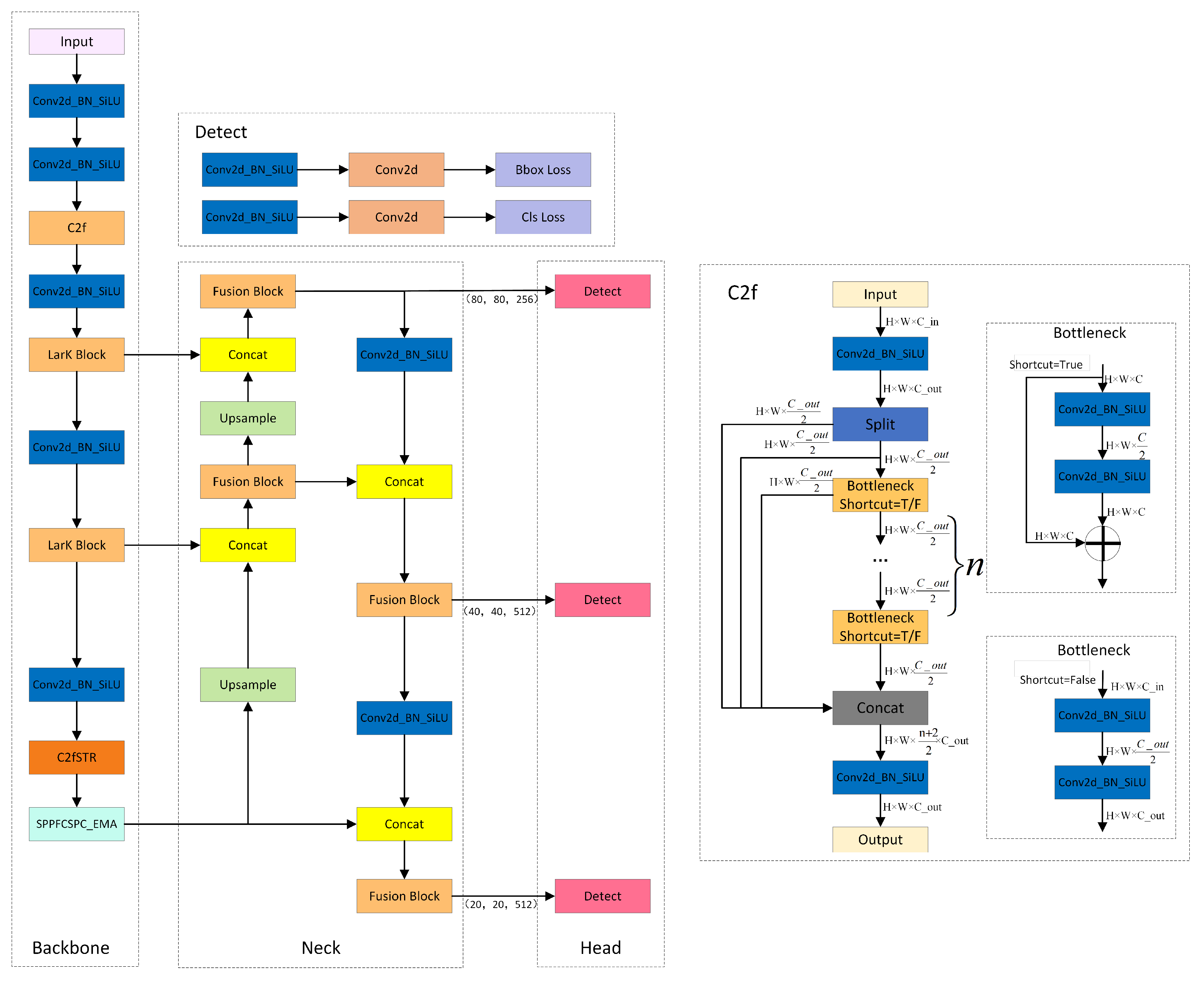
Although the YOLOv8 model has achieved significant results in the field of object detection, there are still some limitations. Firstly, the model’s receptive field during the detection process is relatively limited. At the same time, the feature representation and perception capabilities of the YOLOv8 network need enhancement. Secondly, the diversity of marine life, along with its myriad forms and shapes, poses challenges to the accuracy and robustness of target detection. Lastly, the common absorption and scattering effects of water on light often result in inadequate clarity of target boundary information, hindering precise localization. To address these issues, we designed YOLOv8-MU, as shown in
Figure 1.
3.1. LarK Block
The Convolutional Neural Network (ConvNet) with large kernels has shown remarkable performance in capturing sparse patterns and generating high-quality features, but there is still considerable room for exploration in its architectural design. While the Transformer model has demonstrated powerful versatility across multiple domains, it still faces some challenges and limitations in terms of computational efficiency, memory requirements, interpretability, and optimization. To address these limitations, we introduce the LarK Block from UniRepLKNet into our model [
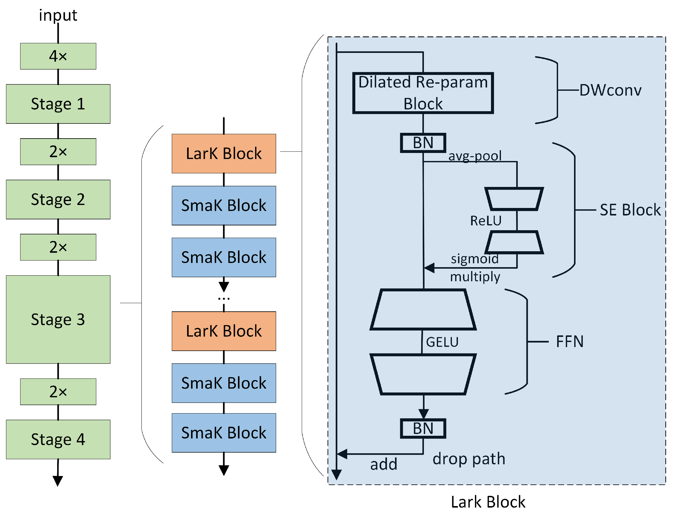
9], as depicted in
Figure 2. It leverages the advantages of large-kernel convolution, allowing us to achieve a larger receptive field without increasing model depth. This implies that by using larger convolutional kernels, the Large Kernel Block can capture more contextual information without the need to add more network layers. This represents a key advantage of large-kernel convolution, enabling the network to capture richer features.
As illustrated in
Figure 2, the block utilizing Dilated Reparam Block is referred to as a Large Kernel Block (LarK Block), while those employing DWconv are termed Small Kernel Block (SmaK Block). The Dilated Reparam Block is proposed based on equivalent transformation, aiming to enhance feature extraction by combining a non-sparse large-kernel convolutional layer with multiple sparse small-kernel convolutional layers. The key hyperparameters of this method include the size of the large kernel K, the size of parallel convolutional layers k, and the sparsity rate r. Assuming there are four parallel layers with K=9, r=(1,2,3,4), and k=(5,3,3,3). To utilize a larger K, more layers can be enhanced by increasing the kernel size or expanding the sparsity rate. For instance, when K=13, five layers are employed with k=(5,7,3,3,3) and r=(1,2,3,4,5), resulting in equivalent kernel sizes of (5,13,7,9,11) respectively. During the inference stage, to transform the Dilated Reparam Block into a large-kernel transformation layer, each batch normalization (BN) layer is first merged into the preceding transformation layer. Then, each layer with dilation rate r > 1 is transformed into Equation(
1), and all generated kernels are added together with appropriate zero-padding. The Dilated Reparam Block utilizes dilated small-kernel convolutional layers to enhance the non-dilated large-kernel layers. From a parameter perspective, these dilated layers are equivalent to non-dilated convolutional layers with larger sparse kernels, enabling the entire block to be effectively transformed into a single large-kernel convolutional layer.
The Large Kernel Block is primarily integrated into the middle and upper layers of the model to enhance the depth and expressive capability of the model when using large kernel convolutional layers. This enhancement is achieved by stacking multiple SE Block (Squeeze-and-Excitation Block) to deepen the model and utilize 3x3 convolutional layers to extract more complex spatial patterns. Conversely, the Small Kernel Block is used when adding more layers to the model, aiming to increase the depth of the model and extract more complex spatial patterns. We note that besides capturing small-scale patterns, enhancing the ability of large kernel blocks to capture sparse patterns may result in higher-quality features. The demand for capturing this pattern aligns perfectly with the mechanism of dilated convolution [
9]. From the perspective of a sliding window, a dilated convolutional layer with a dilation rate of r will scan the input channels to capture spatial patterns, where the distance between each interested pixel and its neighboring pixels is r - 1. Therefore, we adopt dilated convolutional layers parallel to the large kernel and sum their outputs.
3.2. C2fSTR
The proposed C2fSTR in this paper modifies the original YOLOv8 architecture’s C2f module using the Swin Transformer Block[
11]. Compared to the original C2f module, the modified C2fSTR module facilitates better interaction between strong feature maps and fully utilizes target background information, thereby enhancing the accuracy and robustness of object detection under complex background conditions.
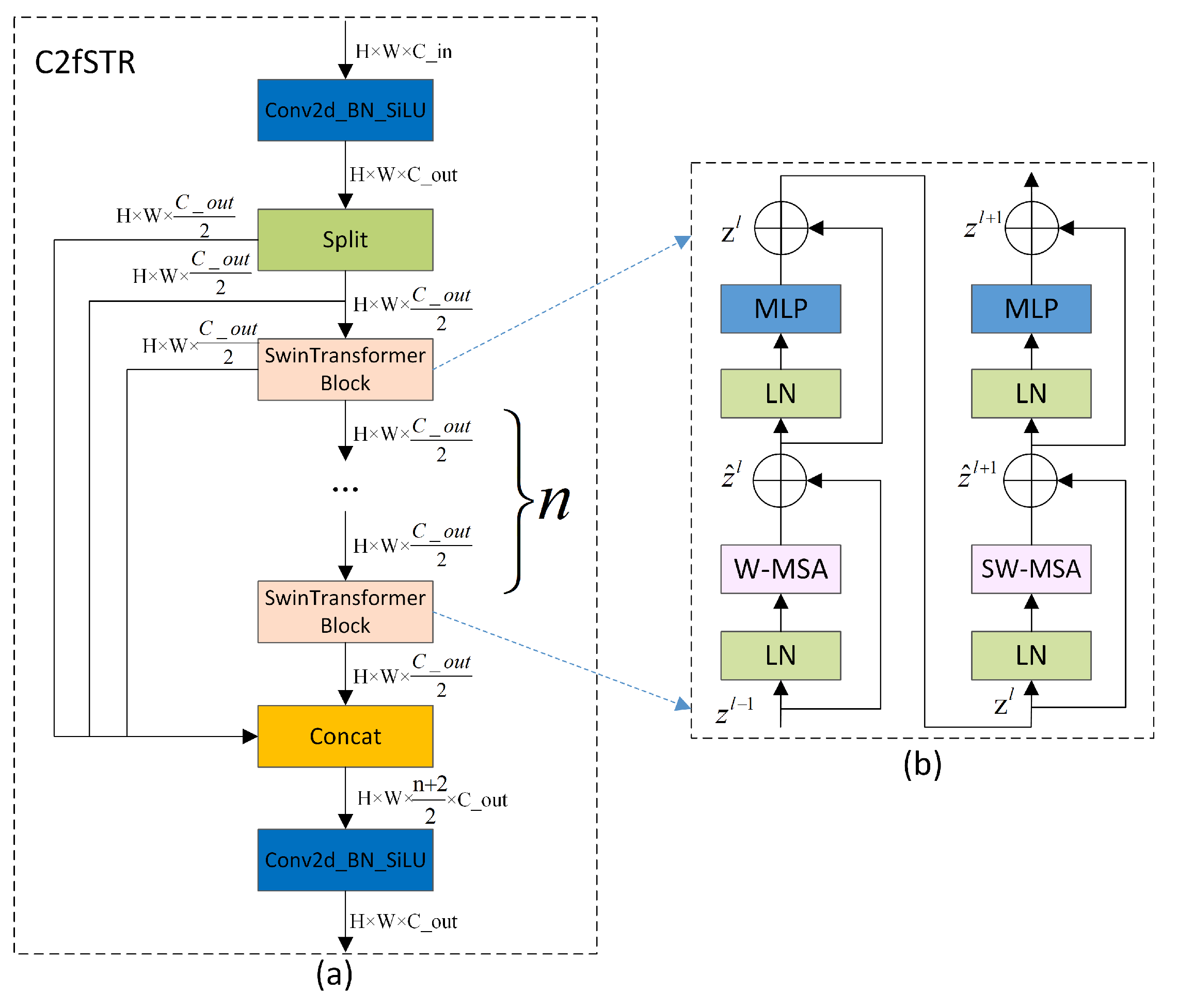
Figure 3.(a) illustrates the structure of the C2fSTR.
The C2fSTR consists of two modules. One is the Conv module, which consists of a Conv2d with a kernel size of 1×1 and a stride of 1, followed by batch normalization and the Silu activation function. The role of the convolution module is to reduce the length and width of the feature map while expanding the dimensionality. The other module is the Swin Transformer Block, which comprises a linear layer (LN), shifted window multi-head self-attention (SW-MSA), and feedforward MLP (MLP). The structure includes n Swin Transformer modules. The function of the Swin Transformer Block is to reduce the computational complexity of the multi-head attention mechanism and expand the range of information interaction. Its structure is illustrated in
Figure 3.(b).
Traditional Transformers typically compute attention globally, leading to high computational complexity. The computational complexity of the multi-head attention mechanism is proportional to the square of the size of the feature map. To reduce the computational complexity of the multi-head attention mechanism and expand the range of information interaction, in the Swin Transformer, the feature map is divided into windows. Each window undergoes window-based multi-head self-attention computation followed by shifted window-based multi-head self-attention computation, enabling mutual communication between windows [
47]. The computation of consecutive Swin Transformer blocks is as Equation(
2):
where
and
represent the output features of the (S)W-MSA and MLP modules of block
l, respectively; W-MSA and SW-MSA represent window-based multi-head self-attention using regular and shifted window partitioning configurations, respectively.
In this way, Swin Transformer effectively reduces the computational burden by confining attention computation within each window. However, object recognition and localization in images depend on the feature information of the global background. The information interaction in Swin Transformer is limited to individual windows and shifted windows, capturing only local details of the target, while global background information is difficult to obtain[
48]. To achieve more extensive information interaction and simultaneously obtain both global background and local detail information, we apply the Swin Transformer Block to C2f, replacing the Darknetbottleneck and forming the C2fSTR feature backbone system. This combined strategy enables comprehensive information interaction, effectively capturing rich spatial details, and significantly improving the model’s accuracy in object detection in complex backgrounds.
3.3. SPPFCSPC_EMA
As shown in
Figure 4, YOLOv8-MU replaces the SPPF module in YOLOv8 with the SPPFCSPC module and introduces multiple convolutions and concatenation techniques to extract and fuse features at different scales, expanding the receptive field of the model and thereby improving model accuracy. Additionally, we have introduced the EMA module, whose parallel processing and self-attention strategy significantly improve the model’s performance and optimize feature representation. By combining the SPPFCSPC and EMA modules to form the SPPFCSPC_EMA module, not only are the model’s accuracy, efficiency, and robustness enhanced, but the model’s performance is further improved while maintaining efficiency.
The SPPFCSPC module integrates two submodules: SPP and fully connected spatial pyramid convolution (FCSPC)[
49]. SPP, as a pooling layer, can handle input feature maps of different scales, effectively detecting both small and large targets. FCSPC is an improved convolutional layer aimed at optimizing the representation of feature maps to enhance detection performance. By performing multi-scale spatial pyramid pooling on the input feature map, the SPP module captures information about targets and scenes at different scales[
37]. Subsequently, the FCSPC module convolves the different scale feature maps output by the SPP module and divides the input feature map into blocks. These blocks are pooled and concatenated, followed by convolution operations, to enhance the model’s receptive field and retain key feature information, thereby improving the model’s accuracy[
49]. The SPPFCSPC module is an optimization of SPPCSPC based on the SPPF concept, reducing the computational requirements for the pooling layer’s output by connecting three independent pooling operations, and improving the speed and detection accuracy of dense targets without changing the receptive field[
50]. The results produced by this pooling method are comparable to those obtained using larger pooling kernels, thus optimizing the training and inference speed of the model. The calculation formula for the pooling part is as Equation (
3):
Where R represents the input feature layer, represents the pooling layer result of the smallest pooling kernel, represents the pooling layer result of the medium-sized pooling kernel, represents the pooling layer result of the largest pooling kernel, represents the final output result, and ⊛ represents tensor concatenation.
The EMA[
13] mechanism employs three parallel pathways, including two 1×1 branches and one 3×3 branch, to enhance the processing capability of spatial information. In the 1×1 branches, global spatial information is extracted through two-dimensional global average pooling, and the Softmax function is utilized to ensure computational efficiency. The output of the 3×3 branch is directly adjusted to align with the corresponding dimensional structure before the joint activation mechanism, which combines channel features as shown in Equation(
4). An initial spatial attention map is generated through matrix dot product operations, integrating spatial information of different scales within the same processing stage. Furthermore, 2D global average pooling embeds global spatial information into the 3×3 branch, producing a second spatial attention map that preserves precise spatial location information. Finally, the output feature maps within each group are further processed through the Sigmoid function [
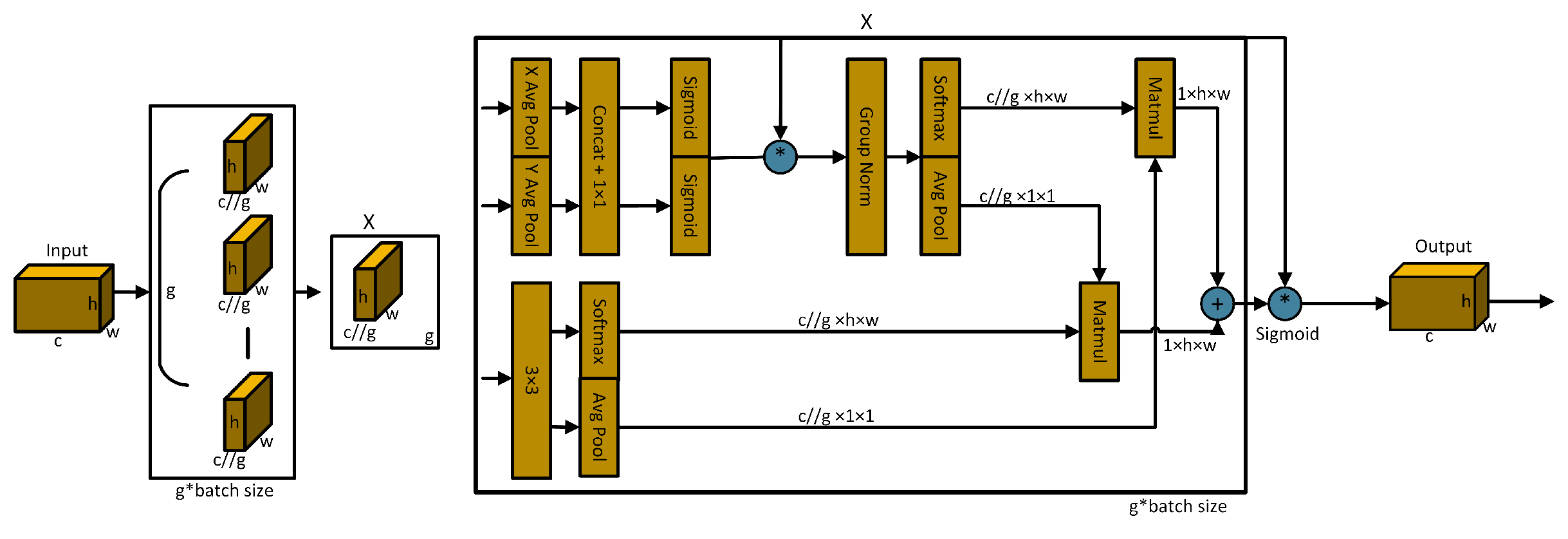
51]. As illustrated in
Figure 5., the design of EMA aims to assist the model in capturing the interactions between features at different scales, thereby enhancing the performance of the model.
Here, represents the output related to the c-th channel. The primary purpose of this output is to encode global information, thereby capturing and modeling long-range dependencies.
Therefore, the overall formula for the SPPFCSPC_EMA module is as shown in Equation(
5):
3.4. Fusion Block
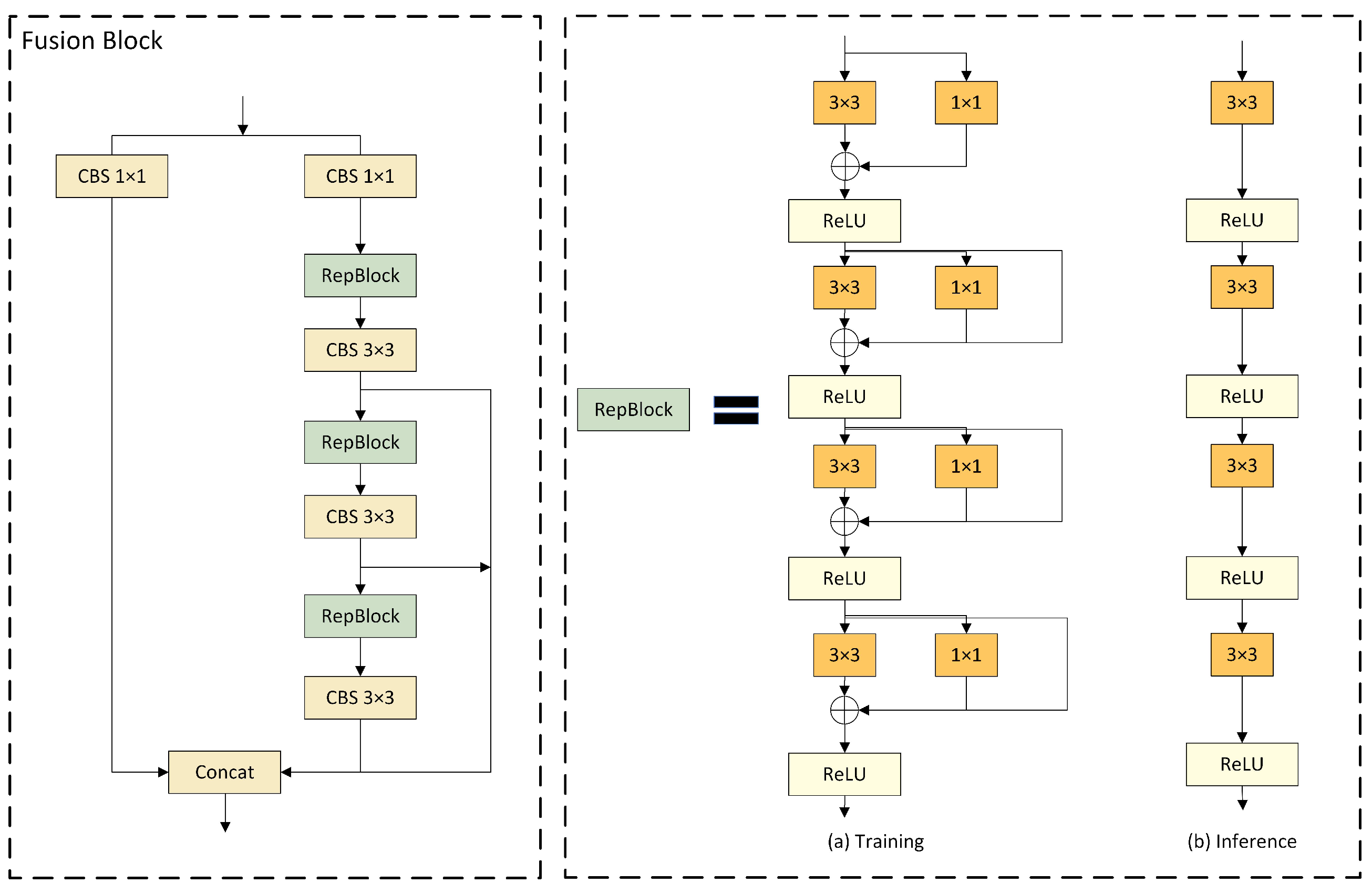
DAMO-YOLO has improved the efficiency of node stacking operations and optimized feature fusion by introducing a specially designed Fusion Block. Inspired by this, we replaced the C2f module in the neck network with the Fusion Block to enhance the fusion capability of multi-scale features. As illustrated in
Figure 6, the architecture of Fusion Block commences with channel number adjustment on two parallel branches through 1 × 1 CBS, followed by the incorporation of the concept of feature aggregation from the Efficient Layer Aggregation Network (ELAN) [
52] into the subsequent branch, comprised of multiple RepBlocks and 3 × 3 CBS. This design leverages strategies such as CSPNet [
53], reparameterization mechanism, and multi-layer aggregation to effectively promote rich gradient flow information at various levels. Furthermore, the introduction of the reparameterized convolutional module has significantly enhanced performance.
In the model, four gradient path fusion blocks are utilized, each splitting the input feature map into two streams. One stream is directly connected to the output, while the other undergoes channel reduction, cross-level edge processing, and convolutional reparameterization before further dividing into three gradient paths from this stream. Ultimately, all paths are merged into the output feature map. This design segments the gradient flow paths, introducing variability in the gradient information as it moves through the network, effectively facilitating a richer flow of gradient information.
As for
Figure 6, RepBlock is designed to employ different network structures during the training and inference phases through the use of reparameterization techniques, thereby achieving efficient model training and rapid inference speed [
54]. Following the recommendations of RepVGG, we optimized the parameter structure, clearly segregating the multi-branch used during the training phase from the single-branch used during the inference phase. During the training process, RepBlock adopts a complex structure containing multiple parallel branches, which extract features through 3x3 convolutions, 1x1 convolutions, and Batch Normalization (BN). This design is intended to enhance the representational capacity of the model. During inference, these multi-branch structures are converted into a single, more streamlined 3x3 convolutional layer through structural reparameterization, eliminating the branch structure to increase inference speed and reduce memory consumption of the model.
The conversion from a multi-branch to a single-branch architecture is primarily motivated by three considerations. Firstly, from the perspective of speed, models reparameterized for inference demonstrate a significant acceleration in inference speed. This not only expedites the model inference process but also enhances the practicality of model deployment. Secondly, regarding memory consumption, the multi-branch model necessitates allocating memory individually for each branch to store its computational results, leading to substantial memory usage. Adopting a single-path model significantly reduces the demand for memory. Lastly, in terms of model flexibility, the multi-branch model is constrained by the requirement that the input and output channels for each branch remain consistent, posing challenges to model modifications and optimizations. In contrast, the single-path model is not subject to such limitations, thereby increasing the flexibility of model adjustments.
3.5. MPDIOU
Existing boundary box regression loss functions, such as CIoU, although considering multiple factors, may still encounter inaccurate localization and blurred boundary issues when dealing with complex scenarios where target boundary information is unclear, affecting the regression accuracy. Given the intricate underwater environment and limited lighting conditions, the boundary information of target objects is often inadequate, posing challenges for traditional loss functions to adapt effectively. Inspired by the geometric properties of a horizontal rectangle, Ma et al. [
16] designed a novel boundary box regression loss function based on the minimum point distance
. We incorporated this function, referred to as MPDIoU, into our model to evaluate the similarity between predicted and ground-truth boundary boxes. Compared to existing loss functions, MPDIoU not only better accommodates blurred boundary scenarios and enhances object detection accuracy but also accelerates model convergence and reduces redundant computational overhead, thereby improving the localization and boundary precision for underwater organism detection.
The calculation process of MPDIoU is as follows: Assume and represent the coordinates of the top-left and bottom-right points of the ground truth box, respectively; and represent the coordinates of the top-left and bottom-right points of the predicted box, respectively. Parameters w and h represent the width and height of the input image, respectively. The formulas for the ground truth box and the predicted box are: and .
Subsequently, the final
can be calculated using Equations (
6) and (
7) based on
and
.
The MPDIoU loss function optimizes the similarity measurement between two bounding boxes, enabling it to adapt to scenarios involving both overlapping and non-overlapping bounding box regression. Moreover, all components of the existing bounding box regression loss functions can be represented using four-point coordinates, as shown in Equations (
8)-(
10).
where
represents the area of the smallest bounding rectangle encompassing both the ground truth and predicted boxes. The center coordinates of the ground truth and predicted boxes are denoted by
and
, respectively, while their widths and heights are represented by and , respectively. Through Equations (
8)-(
10), we can calculate the non-overlapping area, the distance between center points, and the deviation in width and height. This method not only ensures comprehensiveness but also simplifies the computational process. Therefore, in the localization loss part of the YOLOv8-MU model, we choose to use the MPDIoU function to calculate the loss, to enhance the model’s localization accuracy and efficiency.
Author Contributions
Conceptualization, J.Z. ; methodology, X.Z. and J.Z.; software, J.C., X.J. and X.Z. ; validation, X.J., X.Z. and J.C.; formal analysis, X.J.; investigation, J.C.; resources, J.Z.; data curation, X.Z. ; writing—original draft preparation, X.J., X.Z. and J.C., and Y.Z.; writing—review and editing, J.Z.; visualization, X.J. ; supervision, J.Z.; project administration, J.Z.; funding acquisition, J.Z. All authors have read and agreed to the published version of the manuscript.
Figure 1.
The structure of YOLOv8-MU. It consists of Backbone, Neck, and Head, including detailed structures of C2f and Detect.
Figure 1.
The structure of YOLOv8-MU. It consists of Backbone, Neck, and Head, including detailed structures of C2f and Detect.
Figure 2.
The structural design of UniRepLKNet. The LarK Block consists of a Dilated Reparam Block, SE Block [
45], Feed-Forward Network (FFN), and Batch Normalization (BN) [
46] layers. The only difference between the SmaK block and the LarK Block is that the former uses a depth-wise 3×3 convolutional layer to replace the Dilated Reparam layer of the latter. The stages are connected by downsampling blocks, which are implemented by stride-2 dense 3×3 convolutional layers.
Figure 3.
(a) The structure of C2fSTR; (b) Two consecutive Swin Transformer Blocks (represented by Equation (
1)). W-MSA and SW-MSA are multi-head self-attention modules, employing regular and shifted window configurations, respectively.
Figure 3.
(a) The structure of C2fSTR; (b) Two consecutive Swin Transformer Blocks (represented by Equation (
1)). W-MSA and SW-MSA are multi-head self-attention modules, employing regular and shifted window configurations, respectively.
Figure 4.
The structure of SPPFCSPC_EMA. SPPFCSPC performs a series of convolutions on the feature map, followed by max-pooling and fusion over four receptive fields (one 3 × 3 and three 7 × 7). After further convolution, it is fused with the original feature map, and finally combined with EMA to form the SPPFCSPC_EMA module. (Conv: convolution; MaxPool2d: max pooling).
Figure 5.
Schematic diagram of EMA. Here, ’g’ denotes grouping, ’X Avg Pool’ represents 1D horizontal global pooling, and ’Y Avg Pool’ represents 1D vertical global pooling.
Figure 5.
Schematic diagram of EMA. Here, ’g’ denotes grouping, ’X Avg Pool’ represents 1D horizontal global pooling, and ’Y Avg Pool’ represents 1D vertical global pooling.
Figure 6.
Structure diagram of the Fusion Block, which includes a schematic diagram of the RepBlock. (a) represents the model structure used during training, (b) represents the model structure used during inference
Figure 6.
Structure diagram of the Fusion Block, which includes a schematic diagram of the RepBlock. (a) represents the model structure used during training, (b) represents the model structure used during inference
Figure 7.
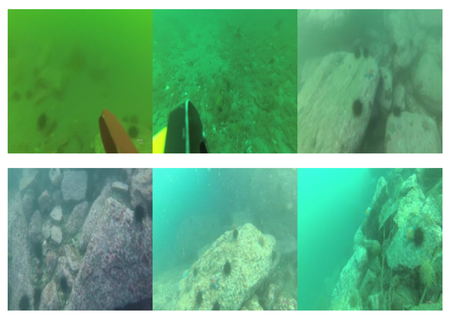
Example images from the URPC2019 and URPC2020 datasets.
Figure 7.
Example images from the URPC2019 and URPC2020 datasets.
Figure 8.
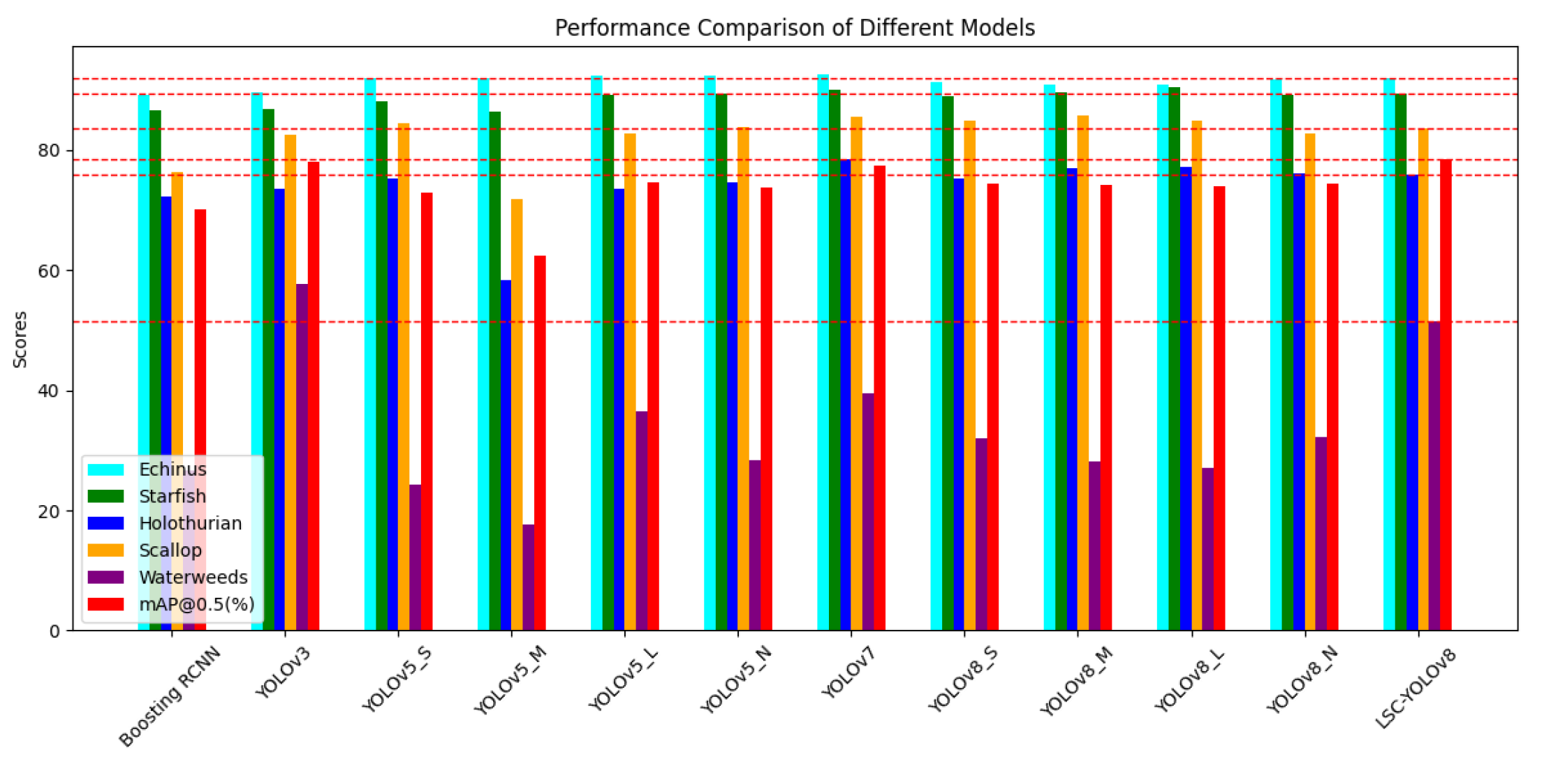
Performance comparison of various models on the URPC2019 dataset.
Figure 8.
Performance comparison of various models on the URPC2019 dataset.
Figure 9.
Performance comparison of various models on the URPC2019 dataset.
Figure 9.
Performance comparison of various models on the URPC2019 dataset.
Figure 10.
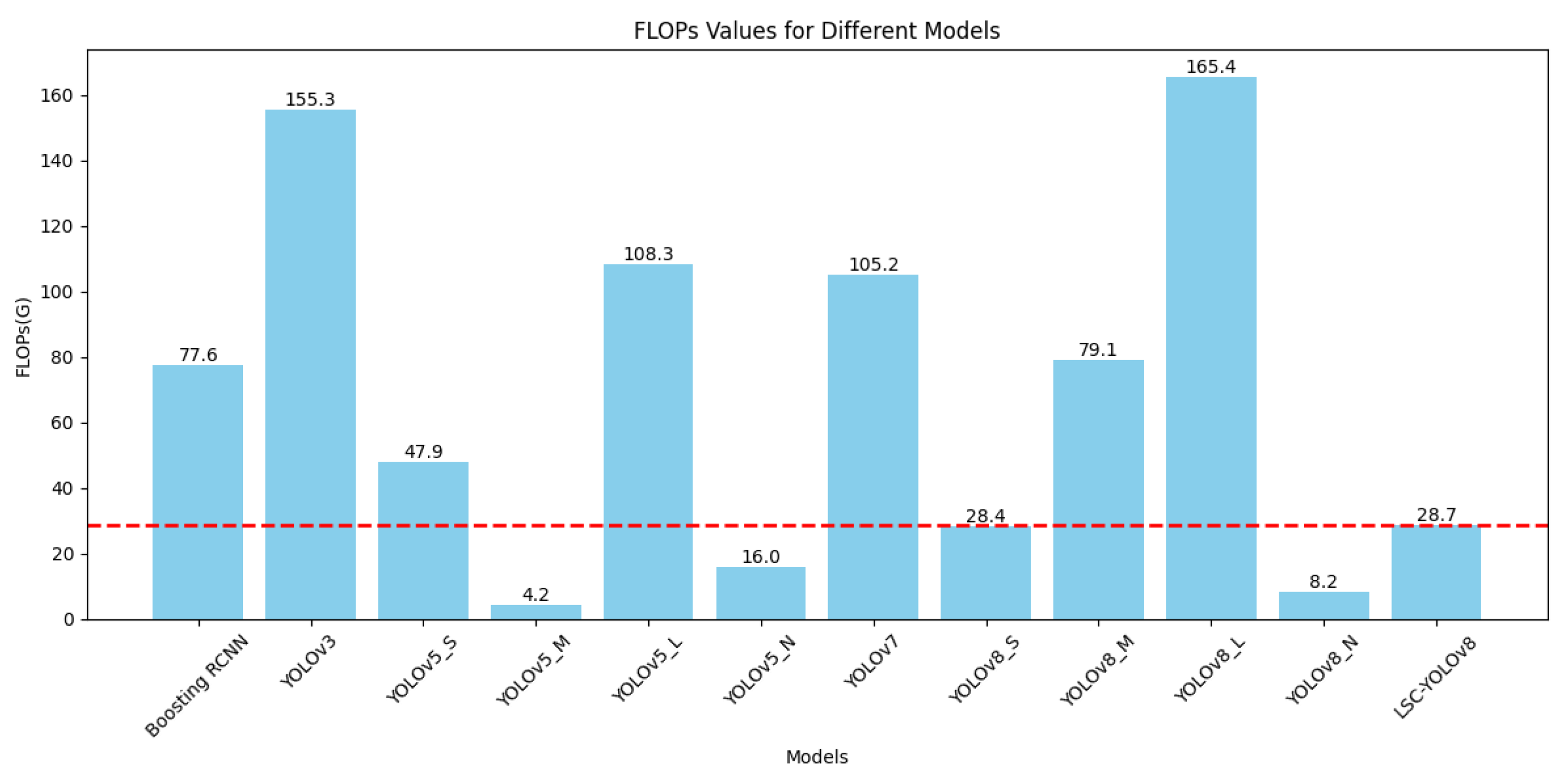
Bar graph comparison of FLOPs for various models on the URPC2019 dataset.
Figure 10.
Bar graph comparison of FLOPs for various models on the URPC2019 dataset.
Figure 11.
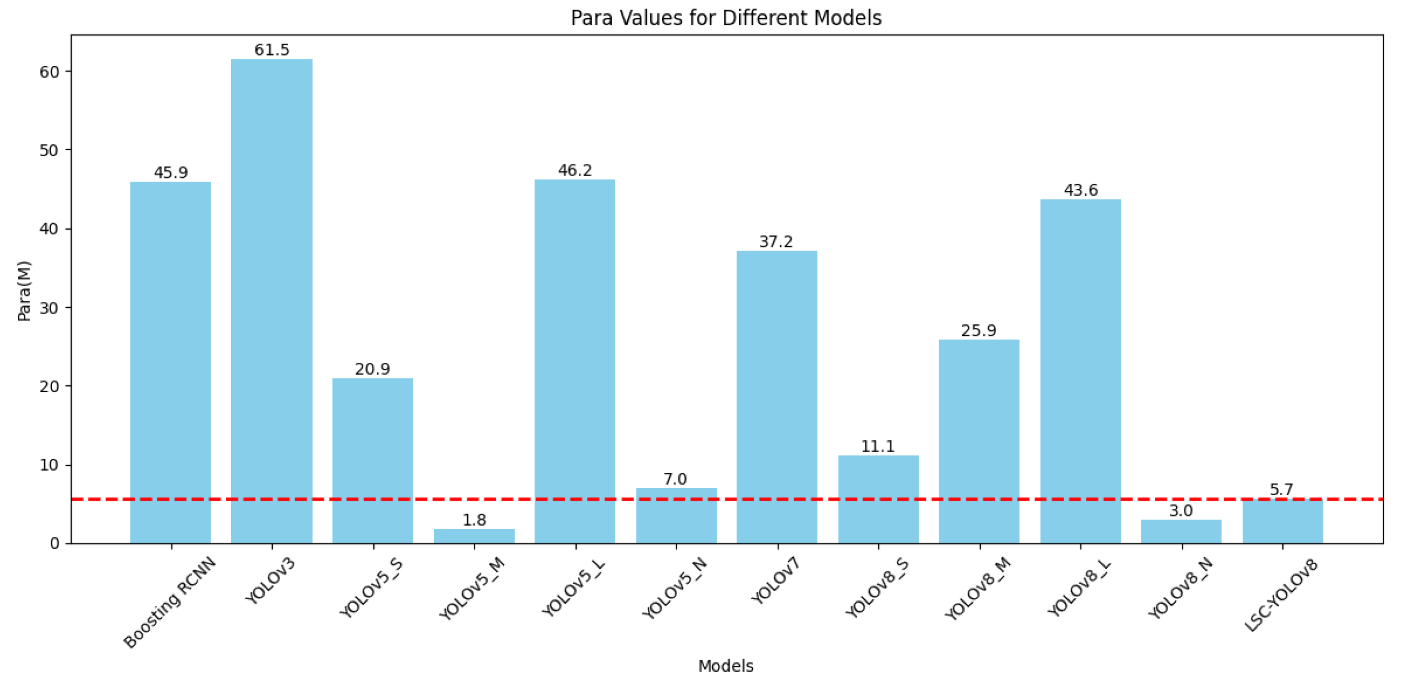
Bar graph comparison of the number of parameters for various models on the URPC2019 dataset.
Figure 11.
Bar graph comparison of the number of parameters for various models on the URPC2019 dataset.
Figure 12.
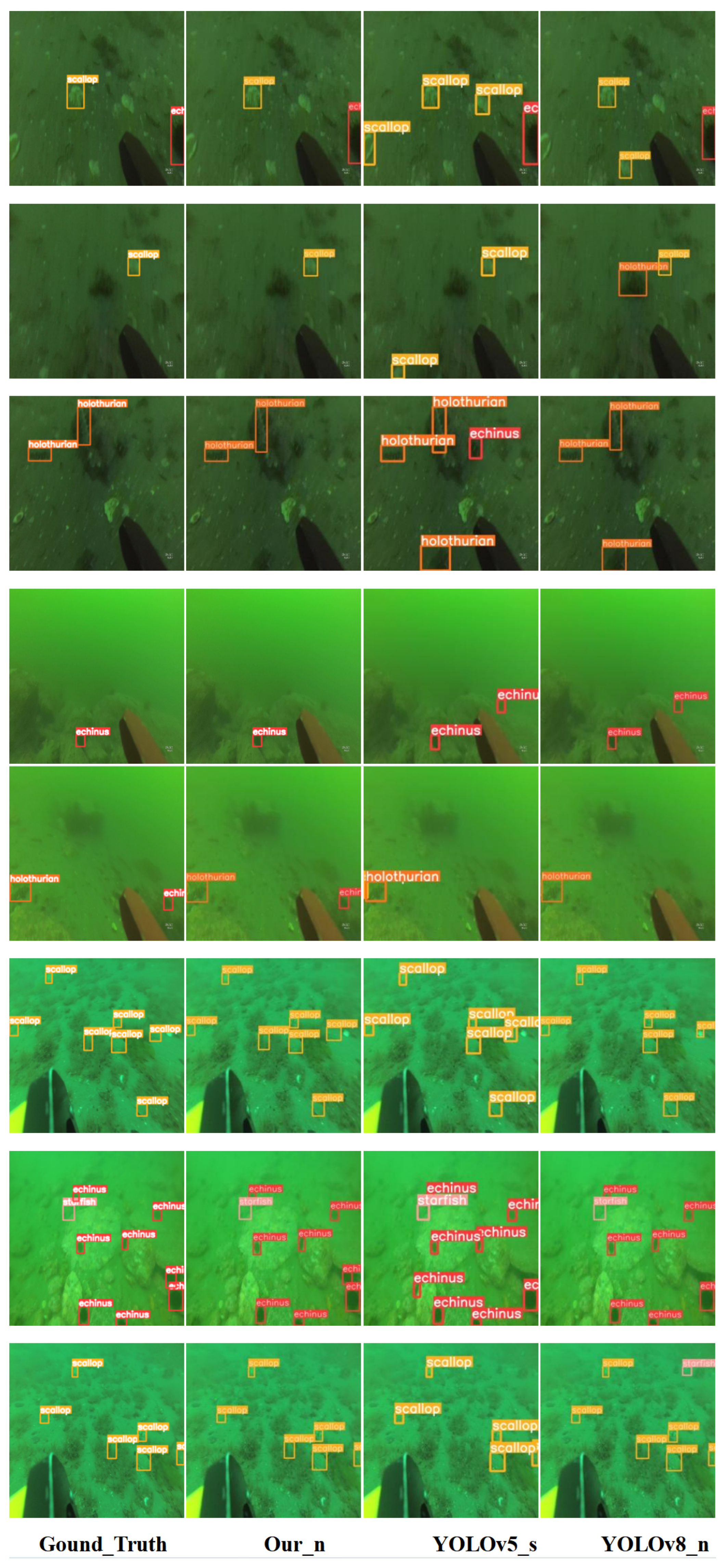
Comparison of target detection results between different models.
Figure 12.
Comparison of target detection results between different models.
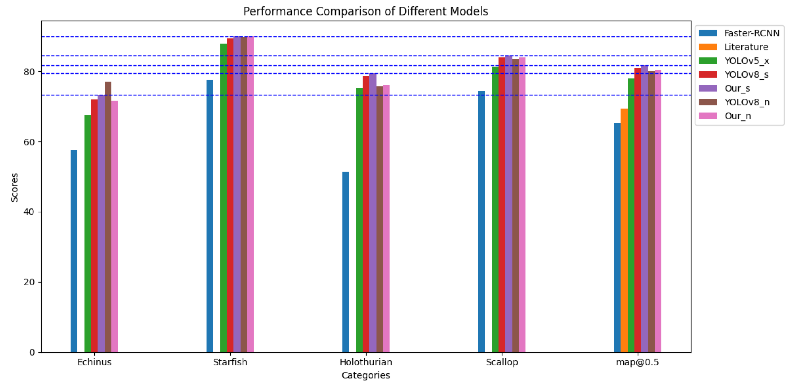
Figure 13.
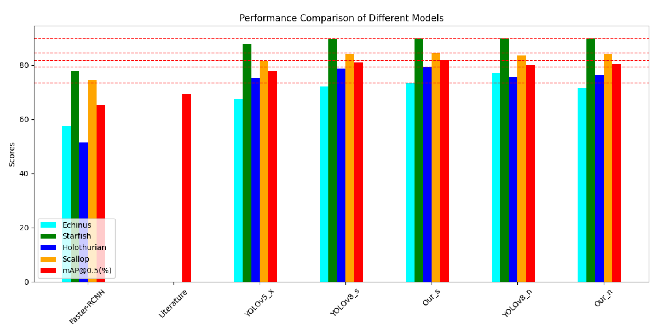
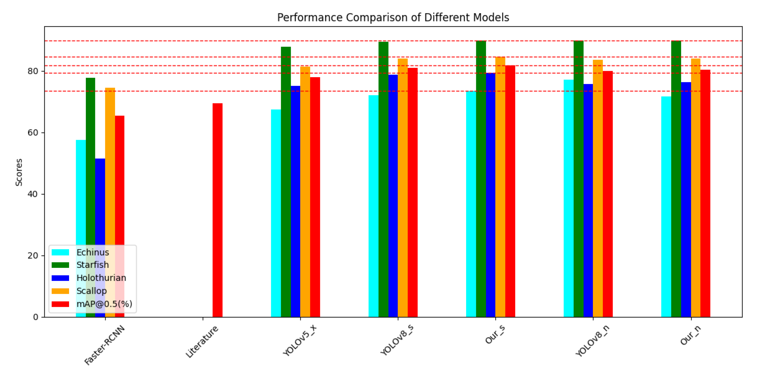
Performance comparison of various models on the URPC2020 dataset.
Figure 13.
Performance comparison of various models on the URPC2020 dataset.
Figure 14.
Performance comparison of various models on the URPC2020 dataset.
Figure 14.
Performance comparison of various models on the URPC2020 dataset.
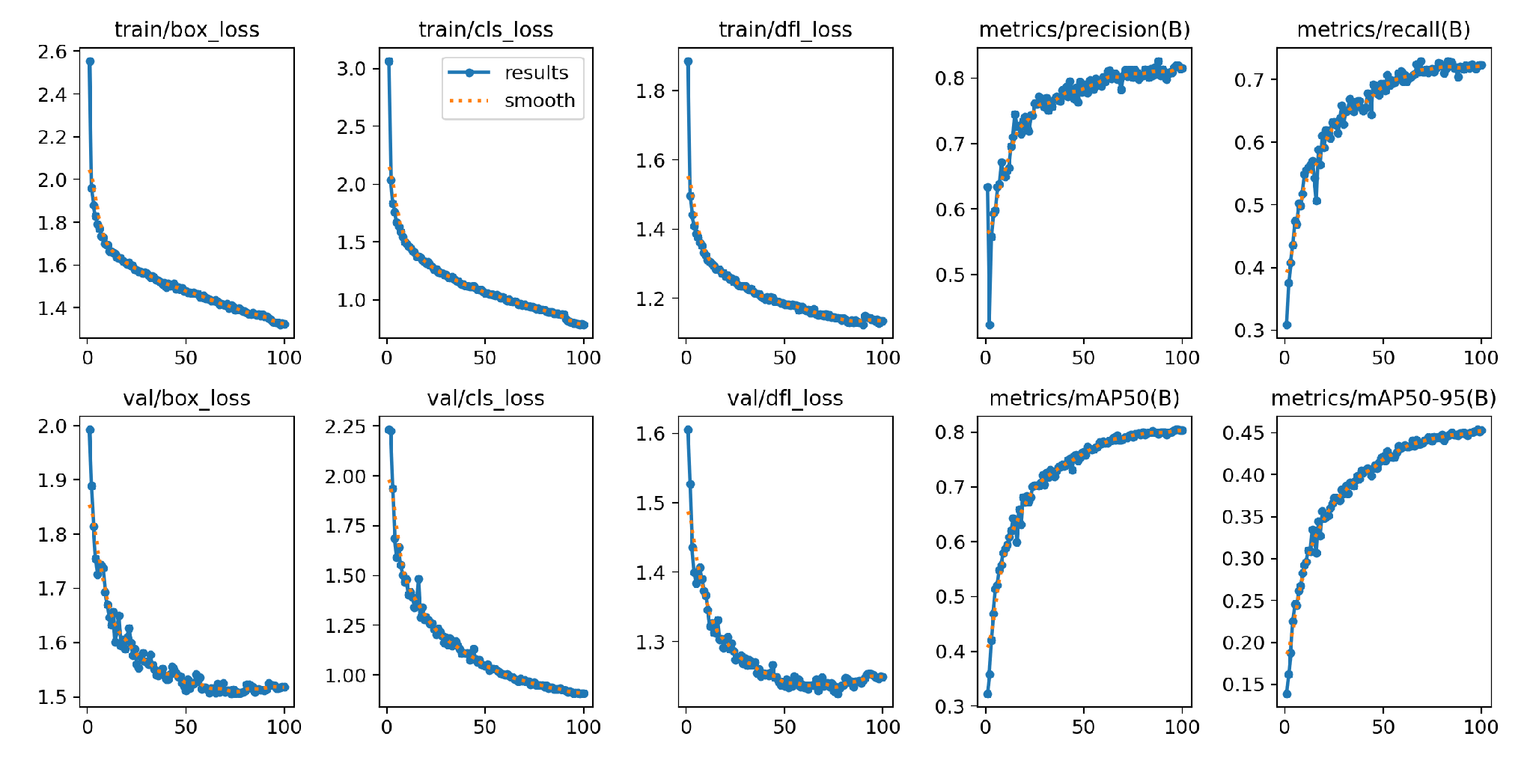
Figure 15.
Results of the YOLOv8-MU model on the URPC2020 dataset.
Figure 15.
Results of the YOLOv8-MU model on the URPC2020 dataset.
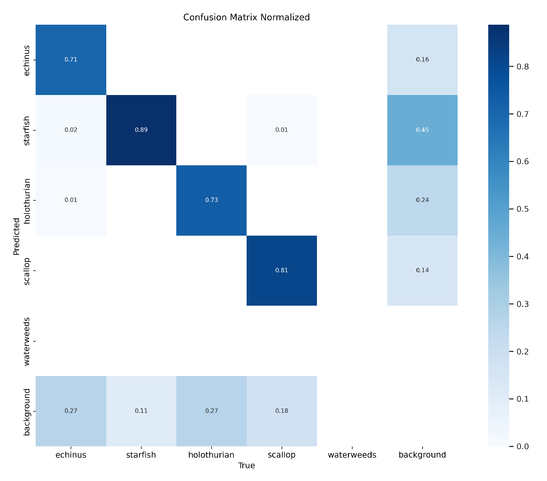
Figure 16.
Confusion matrix of the YOLOv8-MU model on the URPC2020 datasets.
Figure 16.
Confusion matrix of the YOLOv8-MU model on the URPC2020 datasets.
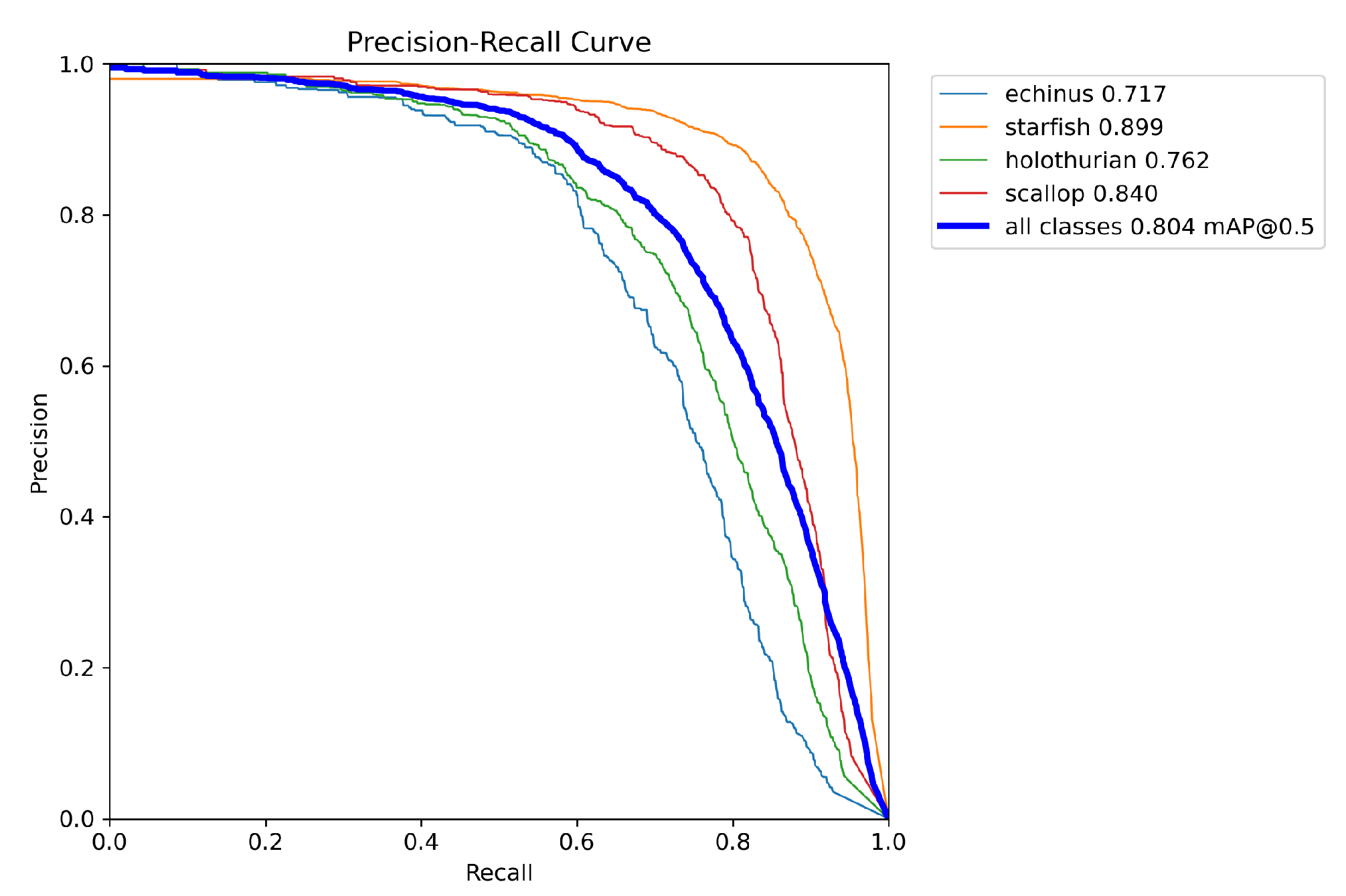
Figure 17.
PR curve of the YOLOv8-MU model on the URPC2020 dataset.
Figure 17.
PR curve of the YOLOv8-MU model on the URPC2020 dataset.
Table 1.
Experimental Environment Configuration.
Table 1.
Experimental Environment Configuration.
| Parameters |
Setup |
| Ubuntu |
20.04 |
| PyTorch |
1.11.0 |
| Python3 |
3.8 |
| CUDA |
11.3 |
| CPU |
12 vCPU Intel(R) Xeon(R) Platinum 8255C CPU @ 2.50GHz |
| GPU |
RTX 3090(24GB) × 1 |
| RAM |
43GB |
Table 2.
Settings of Some Hyperparameters During Training.
Table 2.
Settings of Some Hyperparameters During Training.
| Parameters |
Setup |
| Epoch |
100 |
| Batch size |
16 |
| NMS IoU |
0.7 |
| Image Size |
640×640 |
| Initial Learning Rate |
|
| Final Learning Rate |
|
| Momentum |
0.937 |
| Weight Decay |
0.005 |
Table 3.
Performance comparison of the YOLOv8-MU model with other models on the URPC2019 dataset.
Table 3.
Performance comparison of the YOLOv8-MU model with other models on the URPC2019 dataset.
| Model |
AP(%) |
mAP@0.5 (%) |
Para (M) |
FLOPs(G) |
| |
Echinus |
Starfish |
Holothurian |
Scallop |
Waterweeds |
|
|
|
| Boosting RCNN[20] |
89.2 |
86.7 |
72.2 |
76.4 |
26.6 |
70.2 |
45.9 |
77.6 |
| YOLOv3 |
89.6 |
86.8 |
73.6 |
82.6 |
57.8 |
78.1 |
61.5 |
155.3 |
| YOLOv5s |
92.0 |
88.1 |
75.2 |
84.5 |
24.2 |
72.8 |
20.9 |
47.9 |
| YOLOv5m |
91.9 |
86.3 |
58.4 |
71.8 |
17.6 |
62.5 |
1.8 |
4.2 |
| YOLOv5ł |
92.4 |
89.1 |
73.6 |
82.8 |
36.6 |
74.6 |
46.2 |
108.3 |
| YOLOv5n |
92.4 |
89.3 |
74.7 |
83.8 |
28.4 |
73.7 |
7.0 |
16.0 |
| YOLOv7 |
92.6 |
90.0 |
78.5 |
85.6 |
39.6 |
77.3 |
37.2 |
105.2 |
| YOLOv8s |
91.3 |
89.0 |
75.2 |
84.9 |
32.1 |
74.5 |
11.1 |
28.4 |
| YOLOv8m |
90.9 |
89.5 |
76.9 |
85.7 |
28.1 |
74.2 |
25.9 |
79.1 |
| YOLOv8l |
90.9 |
90.4 |
77.1 |
84.8 |
27.0 |
74.0 |
43.6 |
165.4 |
| YOLOv8n |
91.7 |
89.2 |
76.1 |
82.8 |
32.3 |
74.4 |
3.0 |
8.2 |
| YOLOv8-MU |
91.9 |
89.3 |
75.8 |
83.5 |
51.5 |
78.4 |
5.7 |
28.7 |
Table 4.
Performance comparison of the YOLOv8-MU model with other models on the URPC2020 dataset.
Table 4.
Performance comparison of the YOLOv8-MU model with other models on the URPC2020 dataset.
| Model |
AP(%) |
mAP@0.5 (%) |
| |
Echinus |
Starfish |
Holothurian |
Scallop |
|
| Faster-RCNN[55] |
57.5 |
77.7 |
51.4 |
74.5 |
65.3 |
| Literature[56] |
- |
- |
- |
- |
69.4 |
| YOLOv5x[55] |
67.5 |
87.9 |
75.1 |
81.4 |
78.0 |
| YOLOv8s |
72.0 |
89.4 |
78.7 |
83.9 |
81.0 |
| Ours |
73.4 |
89.9 |
79.4 |
84.5 |
81.7 |
| YOLOv8n |
77.1 |
89.8 |
75.7 |
83.6 |
80.0 |
| Ourn |
71.7 |
89.9 |
76.2 |
84.0 |
80.4 |
Table 5.
Parameter comparison of replacing C2f with LarK Block at different positions in the backbone.
Table 5.
Parameter comparison of replacing C2f with LarK Block at different positions in the backbone.
| Location of LarK Block |
AP(%) |
mAP@0.5 (%) |
Para (M) |
FLOPs(G) |
| |
Echinus |
Starfish |
Holothurian |
Scallop |
Waterweeds |
|
|
|
| All |
91.5 |
88.0 |
73.5 |
82.1 |
35.8 |
74.2 |
3.4 |
9.7 |
| The last three |
91.8 |
88.8 |
73.0 |
82.6 |
30.1 |
73.3 |
3.4 |
9.3 |
| The last two |
90.7 |
88.8 |
75.2 |
82.8 |
29.4 |
73.4 |
3.4 |
8.7 |
| The last one |
91.7 |
89.5 |
75.6 |
83.6 |
28.9 |
73.9 |
3.2 |
8.2 |
| The middle two |
92.2 |
89.4 |
76.4 |
84.6 |
34.7 |
75.5 |
3.2 |
9.2 |
Table 6.
Parameter comparison of replacing C2f with C2fSTR at different positions in the backbone.
Table 6.
Parameter comparison of replacing C2f with C2fSTR at different positions in the backbone.
| Location of LarK Block |
AP(%) |
mAP@0.5 (%) |
Para (M) |
FLOPs(G) |
| |
Echinus |
Starfish |
Holothurian |
Scallop |
Waterweeds |
|
|
|
| All |
90.5 |
89.1 |
73.6 |
82.1 |
33.8 |
73.8 |
3.0 |
30.9 |
| The last three |
90.9 |
88.6 |
75.5 |
82.3 |
36.2 |
74.7 |
3.0 |
29.9 |
| The last two |
90.4 |
88.9 |
75.4 |
82.8 |
35.0 |
74.5 |
3.0 |
27.8 |
| The last one |
91.4 |
88.9 |
75.7 |
82.4 |
37.6 |
75.2 |
2.9 |
18.1 |
| The middle two |
91.6 |
89.0 |
73.2 |
81.9 |
38.4 |
74.8 |
3.1 |
20.0 |
Table 7.
Parameter comparison of replacing C2f with Fusion Block at different positions in the neck.
Table 7.
Parameter comparison of replacing C2f with Fusion Block at different positions in the neck.
| Location of LarK Block |
AP(%) |
mAP@0.5 (%) |
Para (M) |
FLOPs(G) |
| |
Echinus |
Starfish |
Holothurian |
Scallop |
Waterweeds |
|
|
|
| All |
91.5 |
89.7 |
75.7 |
84.0 |
32.6 |
74.7 |
3.95 |
16.5 |
| The last three |
92.2 |
89.6 |
75.6 |
83.8 |
29.1 |
74.1 |
3.8 |
15.8 |
| The last two |
91.8 |
89.1 |
75.7 |
83.1 |
32.9 |
74.5 |
2.9 |
8.4 |
| The last one |
92.0 |
88.8 |
75.3 |
83.3 |
33.5 |
74.6 |
2.7 |
7.8 |
| The middle two |
92.1 |
89.9 |
75.3 |
83.2 |
26.9 |
73.5 |
2.9 |
8.4 |
Table 8.
Demonstration of the effectiveness of each module in YOLOv8-MU;“✓” indicates that we used this module.
Table 8.
Demonstration of the effectiveness of each module in YOLOv8-MU;“✓” indicates that we used this module.
| Module |
mAP@0.5 (%) |
| Lark Block |
C2fSTR |
SPPFCSPC_EMA |
Fusion Block |
MPDIOU |
|
| |
|
|
|
|
74.4 |
| ✓
|
|
|
|
|
75.5 |
| |
✓
|
|
|
|
75.2 |
| |
|
✓
|
|
|
75.3 |
| |
|
|
✓
|
|
74.7 |
| |
|
|
|
✓
|
74.6 |
| ✓
|
|
|
✓
|
|
75.6 |
| ✓
|
|
|
|
✓
|
75.7 |
| |
✓
|
✓
|
|
|
75.6 |
| |
✓
|
|
✓
|
|
75.6 |
| |
✓
|
|
|
✓
|
75.7 |
| |
|
✓
|
✓
|
|
75.4 |
| |
|
✓
|
|
✓
|
75.6 |
| |
|
|
✓
|
✓
|
75.5 |
| |
✓
|
✓
|
✓
|
|
75.8 |
| ✓
|
|
✓
|
|
✓
|
76.3 |
| ✓
|
|
✓
|
✓
|
|
75.8 |
| |
✓
|
✓
|
|
✓
|
75.8 |
| |
|
✓
|
✓
|
✓
|
75.9 |
| |
✓
|
|
✓
|
✓
|
76.0 |
| ✓
|
✓
|
✓
|
✓
|
|
76.0 |
| ✓
|
✓
|
✓
|
|
✓
|
76.5 |
| |
✓
|
✓
|
✓
|
✓
|
77.6 |
| ✓
|
|
✓
|
✓
|
✓
|
76.4 |
| ✓
|
✓
|
✓
|
✓
|
✓
|
78.4 |
