Submitted:
17 April 2024
Posted:
17 April 2024
You are already at the latest version
Abstract
Keywords:
1. Introduction
2. Geological Background
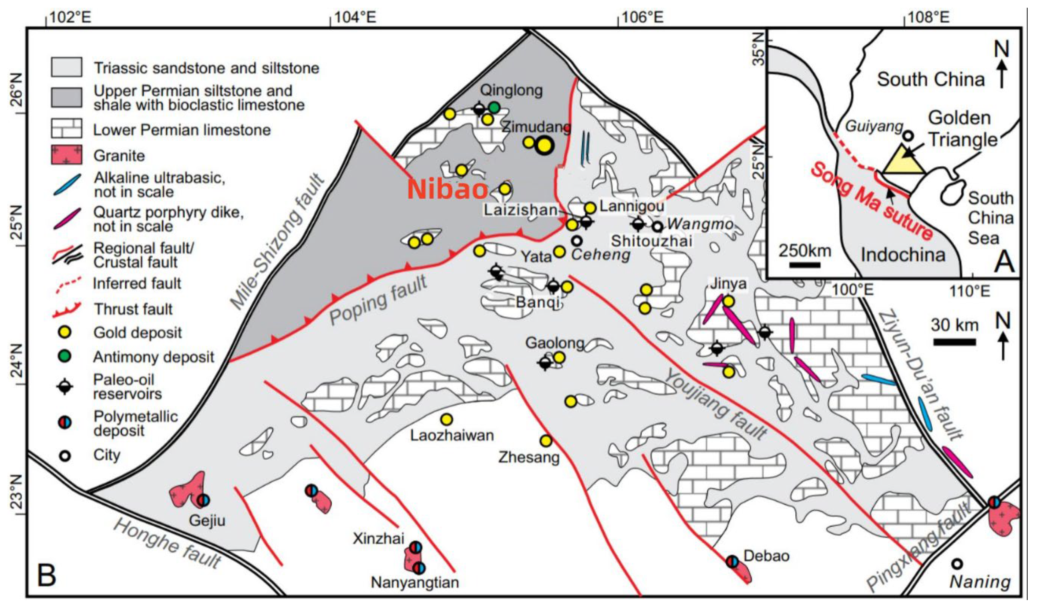
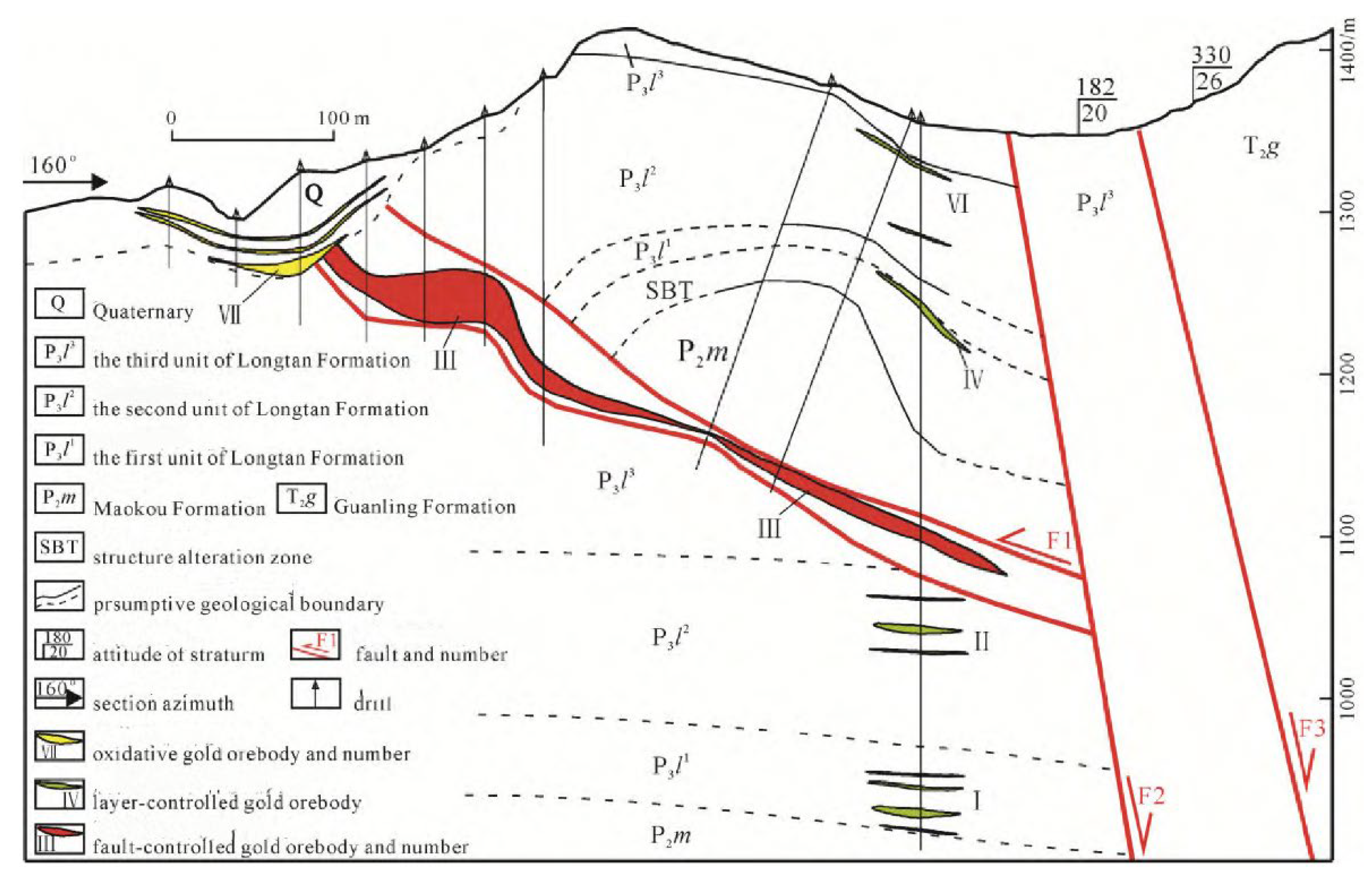
3. Method
3.1. 3D Geological Modeling
| Nugget | Sill | Variation range (m) | Azimuth (°) | Dip Direction (°) | Dip Angle (°) |
| 0.834 | 0.068 | 250.00 | 140.00 | 45.00 | 89.9015 |
3.2. Spatial Analysis
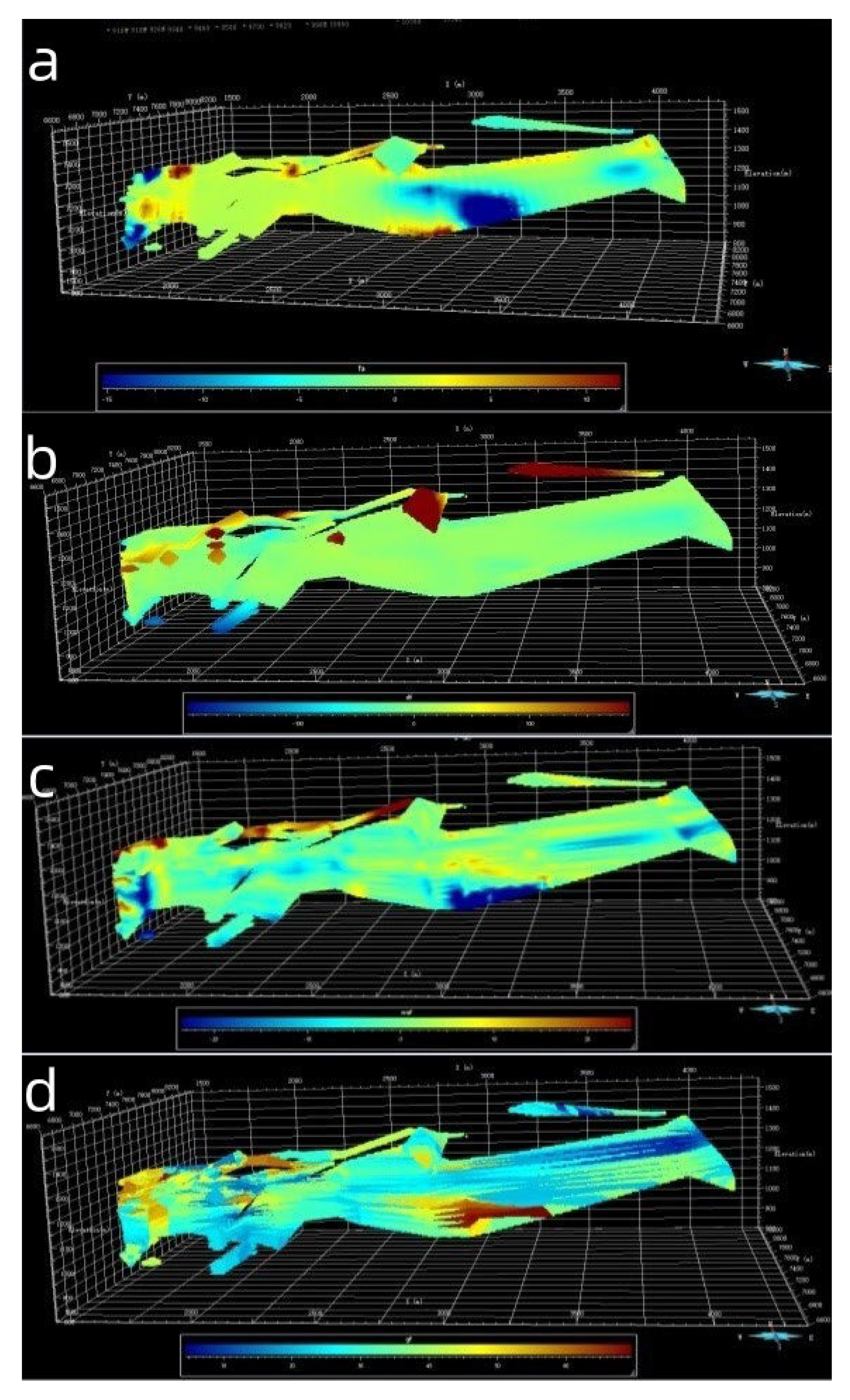
3.3. Mineral Prospectivity Modeling
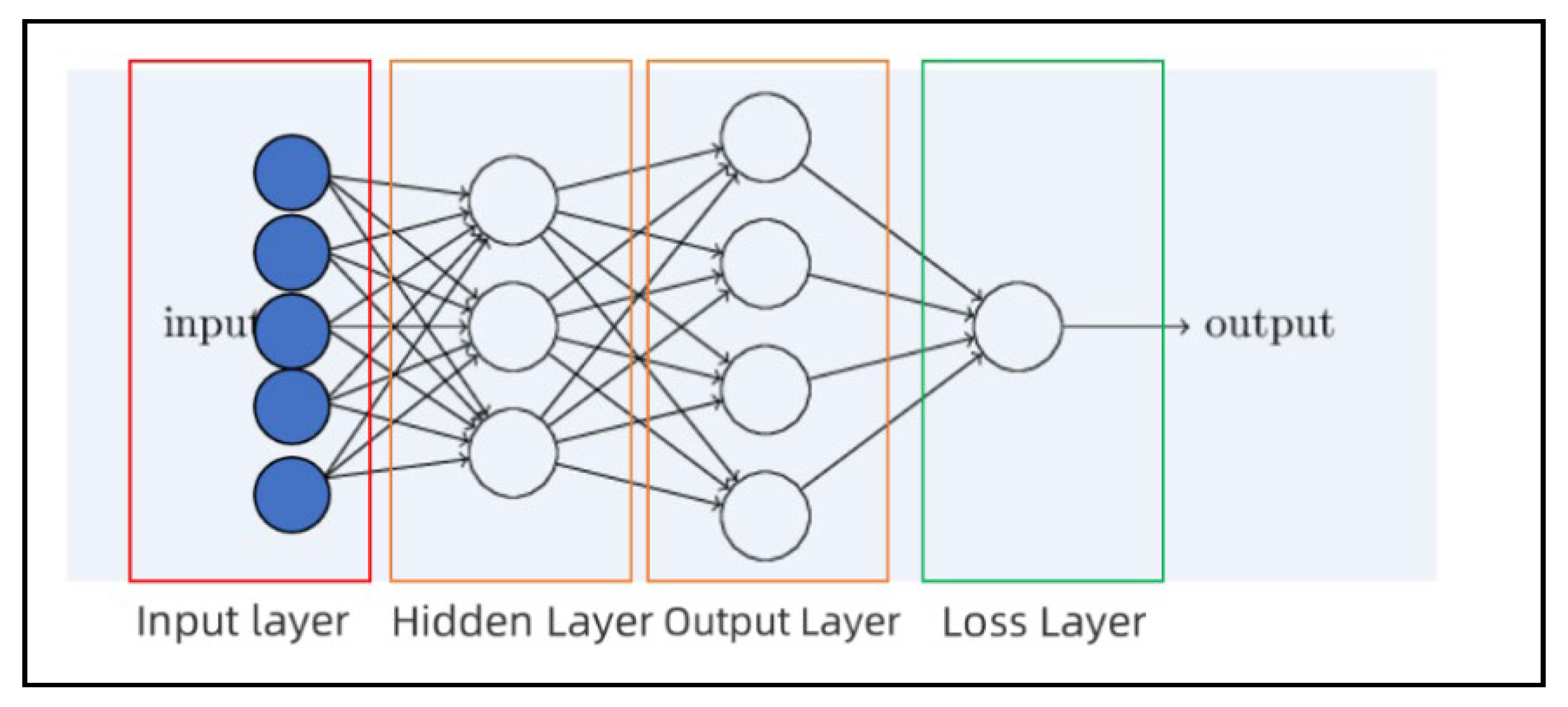
4. Results
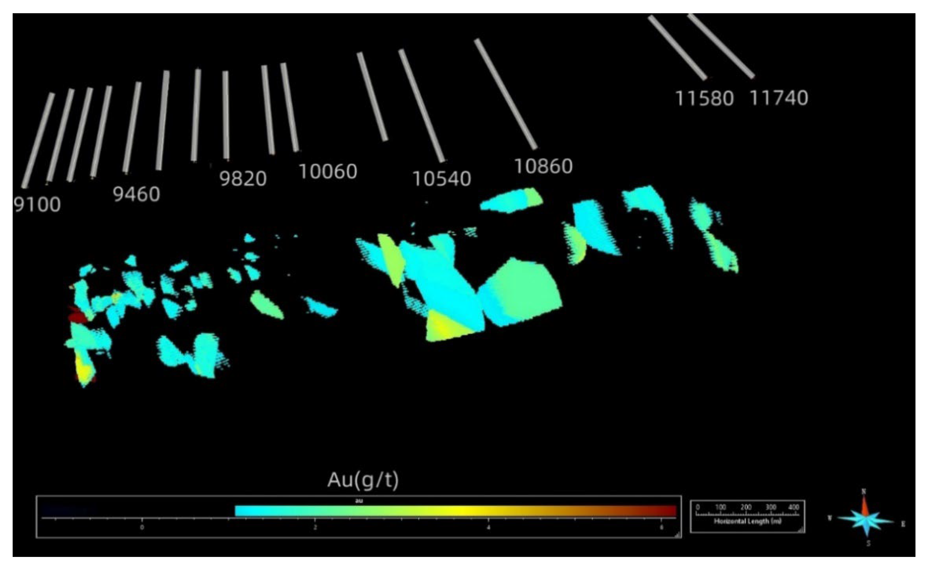
4.1. Spatial Distribution of Gold Mineralization
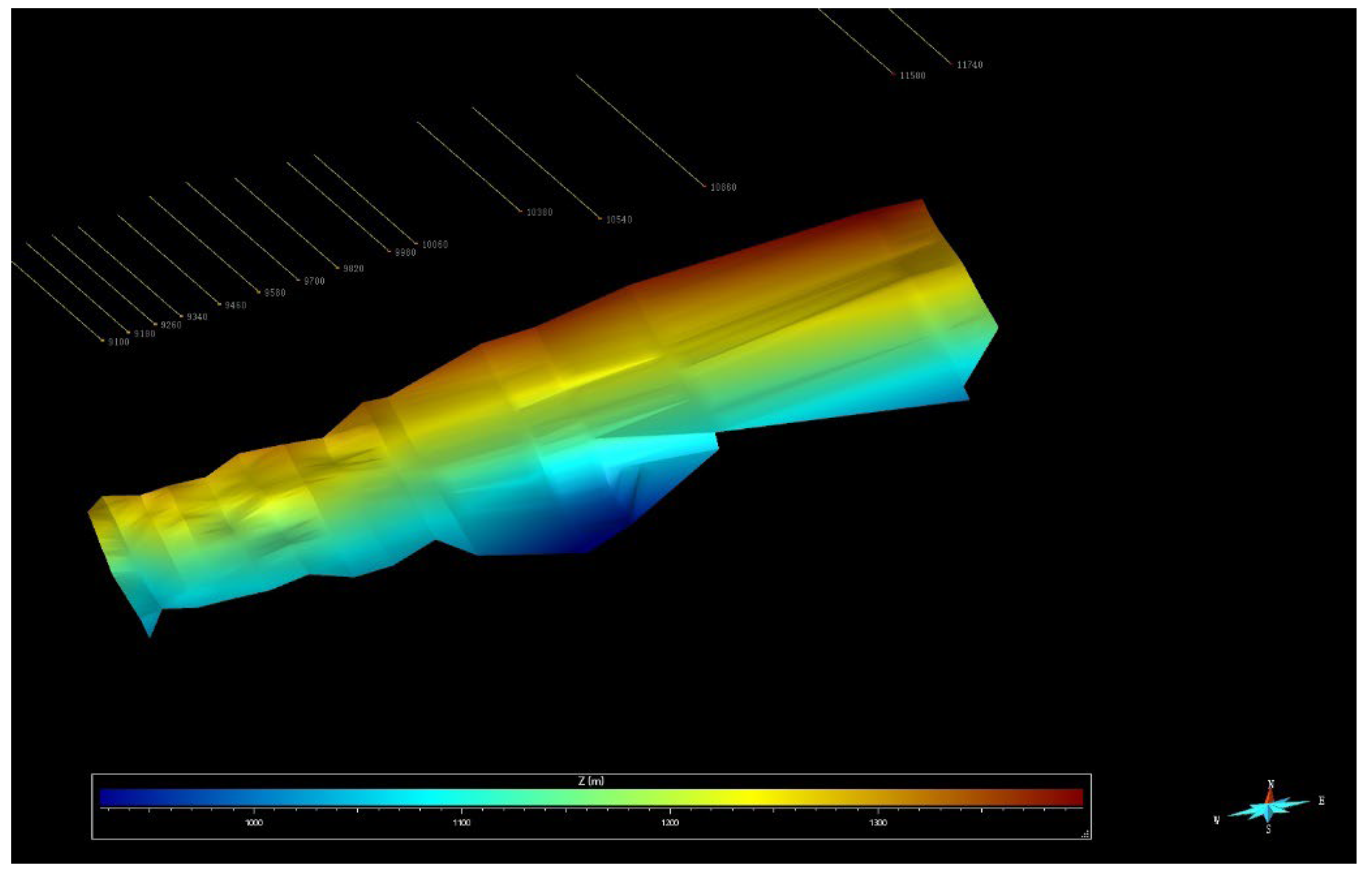
4.2. Structural Deformation in A 3D View
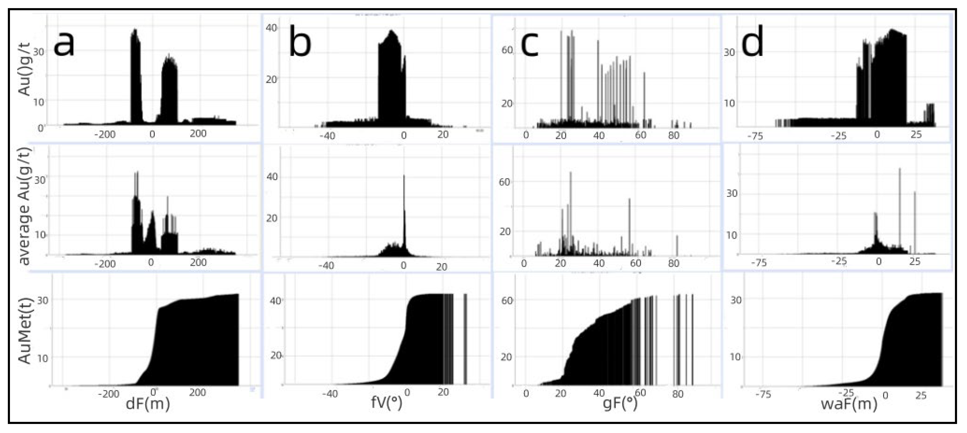
4.3. Correlation between Gold and Structural Features
4.4. Target Appraisal
| Hidden Layer Structure | Optimization Algorithm | Maximum Iterations | Learning Rate | L2 Regularization Parameter / | |
| MLP | [90,90,90,90] | ADAM | 200 | 0.001 | 0.0002 |
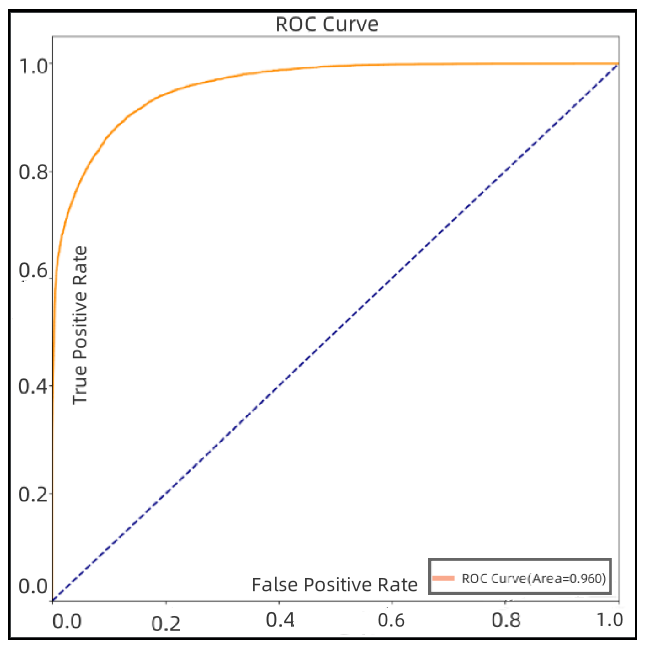
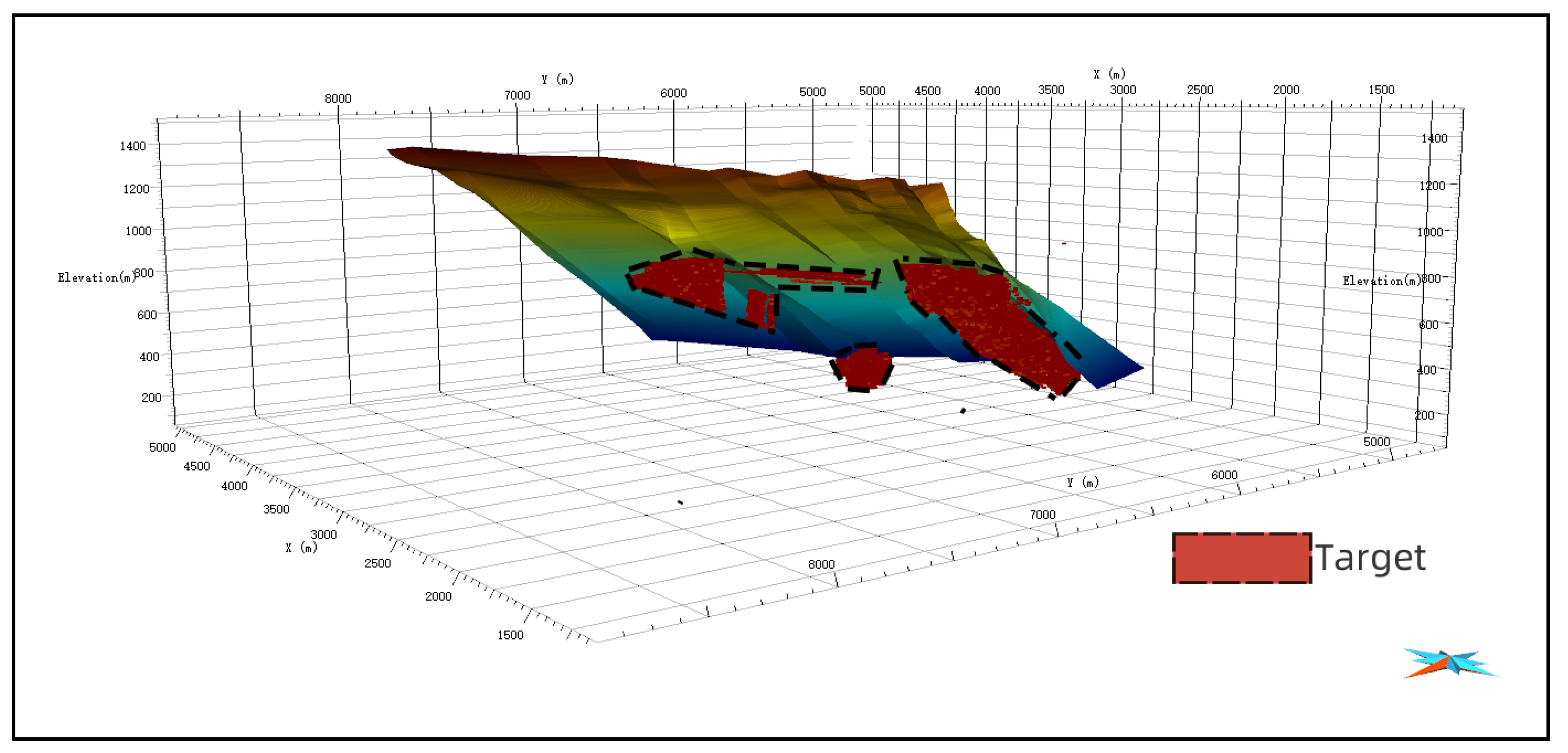
5. Discussion
6. Conclusions
Author Contributions
Funding
Acknowledgments
Conflicts of Interest
References
- Muntean J L, Cassinerio M D, Arehart G B, et al. Fluid pathways at the Turquoise Ridge Carlin-type gold deposit, Getchell district, Nevada[C]//Smart Science for Exploration and Mining, Proceedings of the Tenth Biennial Meeting of the Society of Geology Applied to Mineral Deposits, Townsville, Australia. 2009: 251-252.
- Hofstra A H, Cline J S. Characteristics and models for Carlin-type gold deposits[J]. 2000.
- Cline J S, Hofstra A A. Ore-fluid evolution at the Getchell Carlin-type gold deposit, Nevada, USA[J]. EUROPEAN JOURNAL OF MINERALOGY-STUTTGART-, 2000, 12(1): 195-212.
- Goldfarb, R.J.; Santosh, M. The dilemma of the Jiaodong gold deposits: Are they unique? Geosci. Front. 2014, 5, 139–153. [Google Scholar] [CrossRef]
- Radtke A S, Rye R O, Dickson F W. Geology and stable isotope studies of the Carlin gold deposit, Nevada[J]. Economic Geology, 1980, 75(5): 641-672.
- Kuehn C A, Rose A W. Carlin gold deposits, Nevada; origin in a deep zone of mixing between normally pressured and overpressured fluids[J]. Economic Geology, 1995, 90(1): 17-36.
- Hofstra A H, Cline J S. Characteristics and models for Carlin-type gold deposits[J]. 2000.
- Lamb J B, Cline J. Depths of formation of the Meikle and Betze/Post deposits[J]. 1997.
- Cline J S, Hofstra A H, Muntean J L, et al. Carlin-type gold deposits in Nevada: Critical geologic characteristics and viable models[J]. 2005.
- Hofstra A H, Snee L W, Rye R O, et al. Age constraints on Jerritt Canyon and other Carlin-type gold deposits in the Western United States; relationship to mid-Tertiary extension and magmatism[J]. Economic Geology, 1999, 94(6): 769-802.
- Keith M, Smith D J, Jenkin G R T, et al. A review of Te and Se systematics in hydrothermal pyrite from precious metal deposits: Insights into ore-forming processes[J]. Ore Geology Reviews, 2018, 96: 269-282.
- Groves D I, Goldfarb R J, Gebre-Mariam M, et al. Orogenic gold deposits: a proposed classification in the context of their crustal distribution and relationship to other gold deposit types[J]. Ore geology reviews, 1998, 13(1-5): 7-27.
- Su W, Dong W, Zhang X, et al. Carlin-type gold deposits in the Dian-Qian-Gui “Golden Triangle” of southwest China[J]. 2018.
- Xie Z, Xia Y, Cline J S, et al. Are there Carlin-type gold deposits in China? A comparison of the Guizhou, China, deposits with Nevada, USA, deposits[J]. 2018.
- Mao, X. , Ren, J., Liu, Z., Chen, J., Tang, L., Deng, H., et al. (2019). Three-dimensional prospectivity modeling of the Jiaojia-type gold deposit, Jiaodong Peninsula, Eastern China:A case study of the Dayingezhuang deposit. Journal of Geochemical Exploration, 203, 27–44.
- Payne C E, Cunningham F, Peters K J, et al. From 2D to 3D: Prospectivity modelling in the Taupo volcanic zone, New Zealand[J]. Ore Geology Reviews, 2015, 71: 558-577.
- Mao X, Ren J, Liu Z, et al. Three-dimensional prospectivity modeling of the Jiaojia-type gold deposit, Jiaodong Peninsula, Eastern China: A case study of the Dayingezhuang deposit[J]. Journal of Geochemical Exploration, 2019, 203: 27-44.
- Mao X, Zhang B, Deng H, et al. Three-dimensional morphological analysis method for geologic bodies and its parallel implementation[J]. Computers & Geosciences, 2016, 96: 11-22.
- Xia Y, Su W, Zhang X, et al. Geochemistry and metallogenic model of carlin-type gold deposits in southwest Guizhou province, China[J]. Geochemistry-Earth’s System Processes; Panagiotaras, D., Ed, 2012: 127-156.
- Su W, Dong W, Zhang X, et al. Carlin-type gold deposits in the Dian-Qian-Gui “Golden Triangle” of southwest China[J]. 2018.
- Fu-xin Z, Li X, Ya-lin Q I. Exploration and study of Carlin and Carlin-like type gold deposits: review and prospect[J]. Geology in china, 2004, 31(4): 407-412.
- Xie Z, Xia Y, Cline J S, et al. Are there Carlin-type gold deposits in China? A comparison of the Guizhou, China, deposits with Nevada, USA, deposits[J]. 2018.
- Song W, Zheng L, Liu J, et al. Genesis, metallogenic model, and prospecting prediction of the Nibao gold deposit in the Guizhou Province, China[J]. Acta Geochimica, 2023, 42(1): 136-152.
- Li J, Wu P, Xie Z, et al. Alteration and paragenesis of the basalt-hosted Au deposits, southwestern Guizhou Province, China: Implications for ore genesis and exploration[J]. Ore Geology Reviews, 2021, 131: 104034.
- Xia Y, Su W, Zhang X, et al. Geochemistry and metallogenic model of carlin-type gold deposits in southwest Guizhou province, China[J]. Geochemistry-Earth’s System Processes; Panagiotaras, D., Ed, 2012: 127-156.
- Cline J, S. Timing of gold and arsenic sulfide mineral deposition at the Getchell Carlin-type gold deposit, north-central Nevada[J]. Economic Geology, 2001, 96(1): 75-89.
- Wu Z, Song S, Khosla A, et al. 3d shapenets: A deep representation for volumetric shapes[C]//Proceedings of the IEEE conference on computer vision and pattern recognition. 2015: 1912-1920.
- Pour A B, Hashim M. Structural geology mapping using PALSAR data in the Bau gold mining district, Sarawak, Malaysia[J]. Advances in Space Research, 2014, 54(4): 644-654.
- Malan, DF, Vogler, UW & Drescher K. Time-dependent behaviour of hard rock in deep level gold mines[J]. Journal of the Southern African Institute of Mining and Metallurgy, 1997, 97(3): 135-147.
- Tripp G I, Vearncombe J R. Fault/fracture density and mineralization: a contouring method for targeting in gold exploration[J]. Journal of Structural Geology, 2004, 26(6-7): 1087-1108.
- Carr J C, Beatson R K, Cherrie J B, et al. Reconstruction and representation of 3D objects with radial basis functions[C]//Proceedings of the 28th annual conference on Computer graphics and interactive techniques. 2001: 67-76.
- Houlding, S. 3D geoscience modeling: computer techniques for geological characterization[M]. Springer Science & Business Media, 2012.
- Xiang, J. , Xiao, K., Carranza, E. J. M., Chen, J., & Li, S. (2019). 3D mineral prospectivity mapping with random forests: A case study of Tongling, Anhui China. Natural Resources Research, 29(1), 395–414.
- Xiao, K. Y. , Li, N., Alok, P., Holden, E. J., Leon, B., & Lu, Y. J. (2015). GIS-based 3D prospectivity mapping: A case study of Jiama copper-polymetallic deposit in Tibet, China. Ore Geology Reviews, 71, 611–632.
- Li N, Bagas L, Li X, et al. An improved buffer analysis technique for model-based 3D mineral potential mapping and its application[J]. Ore Geology Reviews, 2016, 76: 94-107.
- Mao, X.; Ren, J.; Liu, Z.; Chen, J.; Tang, L.; Deng, H.; Bayless, R.C.; Yang, B.; Wang, M.; Liu, C. Three-dimensional prospectivity modeling of the Jiaojia-type gold deposit, Jiaodong Peninsula, Eastern China: A case study of the Dayingezhuang deposit. J. Geochem. Explor. 2019, 203, 27–44. [Google Scholar] [CrossRef]
- Allibone A, Teasdale J, Cameron G, et al. Timing and structural controls on gold mineralization at the Bogoso gold mine, Ghana, West Africa[J]. Economic Geology, 2002, 97(5): 949-969.
- Qiu, Y.; Groves, D.I.; McNaughton, N.J.; Wang, L.-g.; Zhou, T. Nature, age, and tectonic setting of granitoid-hosted, orogenic gold deposits of the Jiaodong Peninsula, eastern North China craton, China. Miner. Depos. 2002, 37, 283–305. [Google Scholar] [CrossRef]
- Liu, Z.-K.; Mao, X.-C.; Wang, F.-Y.; Tang, L.; Chen, G.-H.; Chen, J.; Deng, H. Deciphering anomalous Ag enrichment recorded by galena in Dayingezhuang Au(-Ag) deposit, Jiaodong Peninsula, Eastern China. Trans. Nonferrous Met. Soc. China. 2021, 31, 3831–3846. [Google Scholar] [CrossRef]
- Yang, L.Q.; Deng, J.; Guo, R.P.; Guo, L.N.; Wang, Z.L.; Chen, B.H.; Wang, X.D. World-class Xincheng gold deposit: An example from the giant Jiaodong gold province. Geosci. Front. 2016, 7, 419–430. [Google Scholar] [CrossRef]
- Shen, K.; Hu, S.X.; Sun, J.G.; Ling, H.F.; Zhao, Y.Y.; Sun, M.Z. Characteristics of ore-forming fluids of the Dayingezhuang gold deposit in Eastern Shandong, China. Acta Petrol. Sin. 2000, 16, 542–550. [Google Scholar]
- Mao, X.; Zhao, Y.; Deng, H.; Zhang, B.; Liu, Z.; Chen, J.; Zou, Y.; Lai, J. Quantitative analysis of intrusive body morphology and its relationship with skarn mineralization—A case study of Fenghuangshan copper deposit, Tongling, Anhui, China. Trans. Nonferrous Met. Soc. 2018, 28, 151–162. [Google Scholar] [CrossRef]
- Zhang Q, Chen J, Xu H, et al. Three-dimensional mineral prospectivity mapping by XGBoost modeling: A case study of the Lannigou gold deposit, China[J]. Natural Resources Research, 2022, 31(3): 1135-1156.
- Rodriguez-Galiano V, Sanchez-Castillo M, Chica-Olmo M, et al. Machine learning predictive models for mineral prospectivity: An evaluation of neural networks, random forest, regression trees and support vector machines[J]. Ore Geology Reviews, 2015, 71: 804-818.
- Chi G, Xu D, Xue C, et al. Hydrodynamic links between shallow and deep mineralization systems and implications for deep mineral exploration[J]. Acta Geologica Sinica-English Edition, 2022, 96(1): 1-25.
- Yousefi M, Kamkar-Rouhani A, Carranza E J M. Geochemical mineralization probability index (GMPI): a new approach to generate enhanced stream sediment geochemical evidential map for increasing probability of success in mineral potential mapping[J]. Journal of Geochemical Exploration, 2012, 115: 24-35.
- Ruck D W, Rogers S K, Kabrisky M. Feature selection using a multilayer perceptron[J]. Journal of neural network computing, 1990, 2(2): 40-48.
- Popescu M C, Balas V E, Perescu-Popescu L, et al. Multilayer perceptron and neural networks[J]. WSEAS Transactions on Circuits and Systems, 2009, 8(7): 579-588.
- Baum E, B. On the capabilities of multilayer perceptrons[J]. Journal of complexity, 1988, 4(3): 193-215.
- Rasamoelina A D, Adjailia F, Sinčák P. A review of activation function for artificial neural network[C]//2020 IEEE 18th World Symposium on Applied Machine Intelligence and Informatics (SAMI). IEEE, 2020: 281-286.
- Xiong, Y. , & Zuo, R. (2020). Recognizing multivariate geo-chemical anomalies for mineral exploration by combining deep learning and one-class support vector machine. Computers & Geosciences, 140, 104484.
- Xiang, J. , Xiao, K., Carranza, E. J. M., Chen, J., & Li, S. (2019) 3D mineral prospectivity mapping with random forests: A case study of Tongling, Anhui China. Natural Resources Research, 29(1), 395–414.
- Fawcett, T. An introduction to ROC analysis[J]. Pattern recognition letters, 2006, 27(8): 861-874.
- Fawcett, T. ROC graphs with instance-varying costs[J]. Pattern Recognition Letters, 2006, 27(8): 882-891.
- Muschelli III, J. ROC and AUC with a binary predictor: a potentially misleading metric[J]. Journal of classification, 2020, 37(3): 696-708.
- Vuk M, Curk T. ROC curve, lift chart and calibration plot[J]. Metodoloski zvezki, 2006, 3(1): 89.
- Mas J, F. Receiver operating characteristic (ROC) analysis[J]. Geomatic approaches for modeling land change scenarios, 2018: 465-467.
- Ye Z, Kesler S E, Essene E J, et al. Relation of Carlin-type gold mineralization to lithology, structure and alteration: Screamer zone, Betze-Post deposit, Nevada[J]. Mineralium Deposita, 2003, 38: 22-38.
- Yang L, Deng J, Groves D I, et al. Recognition of two contrasting structural-and mineralogical-gold mineral systems in the Youjiang basin, China-Vietnam: Orogenic gold in the south and Carlin-type in the north[J]. Geoscience Frontiers, 2020, 11(5): 1477-1494.
- Nie, A. The study on the genetic mechanism of carlin-type gold deposit which caused by activity of Emei mantle plume in southwestern Guizhou[J]. 2009.
- Song W, Zheng L, Liu J, et al. Genesis, metallogenic model, and prospecting prediction of the Nibao gold deposit in the Guizhou Province, China[J]. Acta Geochimica, 2023, 42(1): 136-152.
- Li J, Wu P, Xie Z, et al. Alteration and paragenesis of the basalt-hosted Au deposits, southwestern Guizhou Province, China: Implications for ore genesis and exploration[J]. Ore Geology Reviews, 2021, 131: 104034.
- Xianyang X, Dingsu F, Maohong C, et al. Fluid inclusion and stable isotope geochemistry study of the Nibao gold deposit, Guizhou and insights into ore genesis[J]. Acta Petrologica Sinica, 2016, 32(11): 3360-3376.
- Zheng L, Yang R, Gao J, et al. Quartz Rb-Sr isochron ages of two type orebodies from the Nibao Carlin-type gold deposit, Guizhou, China[J]. Minerals, 2019, 9(7): 399.
- Jin X, Yang C, Liu J, et al. Source and evolution of the ore-forming fluids of Carlin-type gold deposit in the Youjiang Basin, South China: Evidences from solute data of fluid inclusion extracts[J]. Journal of Earth Science, 2021, 32(1): 185-194.
- Jin X Y, Zhao J X, Feng Y X, et al. Calcite U-Pb dating unravels the age and hydrothermal history of the giant Shuiyindong Carlin-type gold deposit in the golden triangle, South China[J]. Economic Geology, 2021, 116(6): 1253-1265.
Disclaimer/Publisher’s Note: The statements, opinions and data contained in all publications are solely those of the individual author(s) and contributor(s) and not of MDPI and/or the editor(s). MDPI and/or the editor(s) disclaim responsibility for any injury to people or property resulting from any ideas, methods, instructions or products referred to in the content. |
© 2024 by the authors. Licensee MDPI, Basel, Switzerland. This article is an open access article distributed under the terms and conditions of the Creative Commons Attribution (CC BY) license (http://creativecommons.org/licenses/by/4.0/).


