Preprint
Article

Land Management Scale and Carbon Balance Ratio: Spatial Spillover Effects and Threshold Characteristics

Altmetrics

Downloads

59

Views

31

Comments

0

Submitted:

19 April 2024

Posted:

22 April 2024

You are already at the latest version

Alerts
Abstract
The impact of the agriculture net carbon effect is crucial for climate change mitigation, yet research on this topic in China is currently insufficient. In this study, the carbon balance ratio (CBR) is used to characterise the net carbon effect of agriculture, and the spatial Durbin model and threshold regression model were used to empirically analyse the CBR with a sample of 30 provincial-level regions in China from 2004 to 2019. The aim was to investigate the mechanism of the influence of the land management scale (SCALE) of farming on the CBR. The results of the study indicate that national farming generally has a net sink effect, with large changes in interannual fluctuations; the expansion of SCALE has an obvious role in increasing sinks and reducing emissions, and has a positive spatial spillover effect on CBR, with significant spatial heterogeneity. Furthermore, as the SCALE expands, the direction of the influence of rural residents’ income and education level on CBR changes in the opposite direction, showing a significant non-linear relationship characteristic. However, in most areas, the SCALE threshold has not yet been reached, suggesting that the improvement in education levels can still offset the negative impact of economic income growth in the short term. The study recommends paying attention to the role of farmers’ human capital, changing production methods, and implementing carbon peaking and carbon neutrality goals to enhance the net sink effect of the farming industry, which would be achieved by increasing land management scale.
Keywords: 
Subject: Business, Economics and Management  -   Economics

1. Introduction

Human activities, particularly greenhouse gas emissions, have been identified as a clear contributor to global warming [1]. In order to achieve the target of controlling temperature rise to 1.5°C and the global annual greenhouse gas emissions control target, it is recommended that agriculture, forestry, and other land use (AFOLU) CO2 removal should achieve carbon neutrality by around 2030, which is 20 years earlier than the global carbon neutrality goal [2]. Considering China’s pledge at the 75th United Nations General Assembly in September 2020 to reach peak carbon emissions by 2030 and achieve carbon neutrality by 2060, it is important to gain a comprehensive understanding of China’s agricultural carbon sinks. It is worth noting that agriculture can act as both a carbon sink and a source. The agroecosystem is a combination of natural and economic factors, which has been observed to act as a weak carbon sink [3], while the agricultural economic system has been identified as a significant source of greenhouse gas (GHG) emissions [4]. The challenge of achieving carbon peaking and carbon neutrality goals in agriculture, while also absorbing the increasing carbon emissions from other industries, will be a significant test of China’s ability to meet its carbon peaking and carbon neutrality goals as scheduled [5].
Johnson et al. (2007) [6] reviews the literature on GHG emissions and carbon sequestration at the macro level and suggest ways in which agriculture can reduce its GHG footprint and how conservation measures can help to reduce net GHG emissions. Nevertheless, it is worth noting that the integration and analysis of agricultural carbon sinks and emissions has not been widely promoted in the early 21st century. While most studies on carbon emissions by mainland Chinese economists have focused on unilateral carbon emissions, some scholars have begun to expand their research scope as domestic carbon emission accounting methods have become more mature and research conclusions richer.
Over the past decade, there has been an increasing recognition among scholars in the field of agricultural economics that agriculture has dual attributes as both a carbon sink and a carbon emitter. Consequently, more studies have been conducted to examine the net carbon effect in agriculture. At present, research on the net carbon impact of agriculture is primarily concerned with assessing the net carbon sink [7], including its spatial and temporal distribution [8], as well as investigating the factors that affect it [9]. Additionally, certain studies employ various models to examine the correlation between economic development and variables associated with the net carbon sink [10].
A common research approach is to account for both agricultural carbon sinks and emissions, and then subtract the emissions from the sinks to obtain net agricultural carbon sinks for further study [7]. Most studies refer to the “net carbon effect” of Chinese agriculture, as the results tend to be positive in terms of agricultural net carbon sinks. It has been observed that there are varying results in the calculations of the carbon sink effect of Chinese agriculture across different studies. However, it is generally agreed that Chinese agriculture has a net carbon sink effect. According to most studies, it appears that the net carbon sink of Chinese agriculture is increasing [11], as observed through various research methodologies. These differences can be attributed to variations in accounting systems and inconsistent coefficients used in each study. According to existing studies, there is a consensus that Chinese agriculture experiences a significant spatial imbalance in the net carbon sink [12]. Moreover, there are also some studies that are more similar to the idea of accounting for net carbon sinks in agriculture. For instance, one approach is to use the ecological support coefficient (ESC) to express the proportion of carbon sequestration divided by the proportion of carbon emissions [13]. Another method is to calculate the carbon footprint (net carbon emissions) by subtracting carbon sinks from carbon emissions, which can help measure the carbon function of farming in major grain-producing areas [14].
The study of factors influencing net carbon sink and its mechanisms in mainland China has received relatively less attention from scholars due to its late start, and more research is needed, compared with the research on agricultural carbon emissions. Although existing research has provided a good foundation for the study of net carbon sink in agriculture, there is still room for improvement: (1) The research object’s boundary appears to be somewhat ambiguous. While the theses covered a broad range of agricultural topics, such as farming, forestry, animal husbandry, and fisheries, the accounting only seems to have included facility-based animal husbandry and farming. (2) The lack of methodological analysis of impact mechanisms and in-depth study of drivers is a concern. Alterations in land management scale may result in changes in agricultural production methods, which can impact the net carbon sink of agriculture. To draw well-substantiated conclusions, it is essential to have efficient control of natural factors and substantial backing from pertinent economic theories when scrutinizing the impacts. (3) Among the few relevant studies that have examined the factors of influence, there are few analyses that combine spatial and threshold characteristics. Current studies on the net agricultural carbon sink mostly use a single model or method, which limits the accurate estimation of the potential drivers of the net agricultural carbon sink.
This paper explores the carbon balance ratio of the farming industry in 30 regions of China from 2004 to 2019, measuring the net carbon sink and balance ratio. Spatial and threshold models are used to investigate the influence of land management scale on the carbon balance ratio and to analyse the influence mechanism and its causes, which identified deficiencies are taken as an entry point.
The following is an outline of the remaining sections of the paper: Section 2 outlines the theoretical mechanisms by which land management scale, income level, and education level impact the carbon balance ratio, proposing corresponding theoretical hypotheses. In Section 3, variables and data are identified, and econometric models are constructed in baseline, spatial panel, and threshold panel forms. Section 4 briefly presents the explanatory variables and analyses the results of the different econometric models, with a focus on the possible causes of spatial spillovers and the threshold characteristics of rural residents’ income and education levels. Section 5 discusses the results, with a specific focus on exploring the presence and causes of spatial heterogeneity, as well as the threshold values. Lastly, section 6 concludes the paper and offers recommendations based on the findings.

2. Theoretical Mechanisms

2.1. Analysis of the Mechanisms Influencing the Land Management Scale

The carbon sink characteristics of farmland ecosystems are primarily influenced by management measures [15]. Therefore, it would be beneficial to further investigate the mechanism and path of influence of agricultural production methods on the carbon balance of farming. Land and labour are widely recognized as the most fundamental resources in agricultural production. The matching ratio of these resources, commonly referred to as land management scale, is a crucial indicator of agricultural production methods [16].
Achieving carbon balance in farming can be facilitated by optimising land management scale and shifting production methods. The expansion of land management scale in agricultural production often leads to a fundamental shift in production methods, impacting factor inputs, technology applications, and physical outputs. This shift involves a move away from traditional agriculture, which relies on human labour, towards modern agriculture that utilises mechanisation, automation, and intelligence. The transformation has contributed to a reduction in resource waste caused by farmland dispersal and an improvement in production efficiency, which has played a crucial role in controlling the rapid growth of carbon emissions [17]. Large-scale agricultural operations have encouraged farmers to adopt advanced farmland management practices, such as straw return, minimum tillage, and no-tillage, as well as sustainable agricultural practices like crop rotation and cover crops. These measures could potentially increase soil organic matter content and improve the soil’s carbon fixation capacity, which could have a positive impact on the agricultural carbon balance [2]. It is important to note that this impact is based on the assumption that adjusting the land management scale will result in corresponding changes to the agricultural production function. This assumption is relatively easy to meet in the context of China’s current agricultural policies and practices [18]. The government aims to optimize the production function, increase farmers’ profitability, and alleviate the problems of agriculture, rural areas, and farmers (the “Three Rural Issues”) by promoting large-scale agricultural operations. As the land management scale increases, farmers at the micro level tend to adopt innovations in agricultural production methods to improve efficiency.
There may be spatial correlation between agricultural production methods and agricultural management practices across regions. The study by Xiao et al. (2013) [19] supports this conjecture. At the spatial level, it is observed that production factors, such as agricultural materials and technology, tend to flow across regions [20]. The efficiency of this flow is inversely proportional to the distance between regions. Therefore, regions that are in close proximity tend to exhibit similar characteristics in terms of agricultural production activities. This phenomenon is observed worldwide [21]. It is common for neighbouring regions to exchange and implement agricultural production methods and management measures, resulting in a diffusion effect of technology and even a tendency towards homogenisation of agricultural science and technology development [22]. Expanding the land management scale of a region and adopting new technologies and management measures during the transformation of production methods can potentially improve production and land-use efficiency. Furthermore, it may promote the improvement and upgrading of agricultural production methods in neighbouring regions, which can have an impact on the carbon balance of farming in the region as a whole.
Areas with similar conditions may converge and develop due to similar or identical policies. Governments must formulate and implement policies and management measures adapted to the specific conditions of different regions as agricultural production methods change. For instance, in 2004, China designated 13 provinces as major grain-producing provinces, and since then, agricultural industrial policies have been tilted towards these areas. Policies related to main grain-producing areas encompass a range of agricultural policies that provide support and incentives for grain cultivation, as well as the purchase of grain [23]. The establishment of large-scale agricultural operations in grain-producing areas promotes intensive grain production. This is achieved not only by expanding the size of farmers’ plots through land remediation but also by encouraging farmers to shift from multi-species cultivation to specialised cultivation of a single variety of grain [24]. This allows for economies of scale brought about by continuous grain operation in major grain-producing areas and facilitates carbon emission reductions [25].
Therefore, this paper examines the spatial effect of expanding land management scale to increase sinks and reduce emissions, which is significant for coordinating the carbon function of the nation’s farming industry and achieving a nationwide carbon peak. In summary, this paper obtains the first research hypothesis:
Hypothesis 1. The land management scale can directly impact the net carbon effect of farming and has a clear spatial spillover effect.

2.2. Analysis of Threshold Mechanisms

The concept of the environmental Kuznets curve (EKC) suggests an “inverted U-shaped” relationship between environmental pollution and per capita income [26]. Specifically, in the early stages of economic development, environmental pollution tends to increase with per capita income. However, at a certain stage of development, environmental pollution begins to decrease as per capita income continues to rise. The net carbon effect of farming, as a positive representation of the ecological environment, should also have a “U-shaped” relationship between the net carbon effect of farming and rural per capita income if the conditions of the applicable environmental Kuznets curve are met.
The expansion of land management scale is considered a necessary condition for establishing the “U-shaped” curve. However, economic development and income increase alone are not enough to complete the logical derivation. It is worth noting that the emergence of the EKC inflection point is not a natural occurrence of economic development, and economic growth itself does not automatically lead to environmental improvement. The “inverted U-shaped” curve of environmental pollution arises due to economic growth resulting from industrial structure transformation, technological progress, or environmental regulation [27]. It is suggested that changes in land management scale may be more indicative of changes in agricultural production methods than inertial growth in economic output. This implies that the threshold for the inflection point of the “U-shaped” curve, transitioning from negative to positive, may be related to the scale of management. This assumption suggests that at a specific scale of land management (commonly referred to as an “appropriately scaled agricultural operation” in domestic studies) the increase in per capita income no longer has a negative impact on the environment. Instead, it has a positive impact.
One possible explanation for this change is that, as farmers reach a certain scale of land management, they may transition from traditional “survival farmers” to modern “rational farmers” [28]. In the process of maximizing their net returns, they may change their risk-averse mindset of “more fertiliser, more pesticide” and reduce the input intensity of high-carbon emission agricultural materials to effectively control total costs [29]. In the pursuit of maximising their net income, farmers may consider adjusting their approach to the use of agricultural materials. This may involve reducing the intensity of inputs with high carbon emissions, in order to effectively control the total cost of ownership. And here, per capita income is not only a measure of economic development but also the most significant source of reinvestment in agricultural production for farmers [30]. Therefore, the relationship between per capita income and the net carbon effect of farming may be even closer.
The potential influence of education level on the net carbon effect of farming, and how it may vary with the scale of land management, is an aspect of particular interest for this paper. While most studies suggest that higher education levels have a positive impact on improving the ecological environment and reducing carbon emissions [31], Guan et al. (2023) [11] found in their latest study that the education level of rural residents has a non-linear relationship with the net carbon sink in agriculture, even though the accounting method of the explanatory variables in this paper is different from that of theirs. As a result, this paper proposes the second research hypothesis:
Hypothesis 2. The influence of income level and education level on the net carbon effect of agriculture has a significant threshold feature, and only when the land management scale reaches the threshold, the role of income level is transformed into a positive one, while education level instead has a negative effect on it.

3. Materials and Methods

3.1. Variables

3.1.1. Indicator Selection

(1) Carbon balance ratio (CBR): this paper firstly carries out the accounting of net carbon sink (NCS) and carbon balance ratio (CBR), combined with the relevant research results in the field of net carbon sink and carbon ecological carrying capacity coefficient. NCS is obtained by subtracting carbon emission (CE) from carbon sink (CS), and CBR is the result of dividing CS by CE, which characterises the situation of carbon sinks and carbon sources of farming from different perspectives. When CBR is greater than 1, it suggests that the farming industry has a net carbon effect that acts as a sink, providing additional carbon sinks for other industries to offset a portion of their carbon emissions. On the other hand, when CBR is less than 1, it indicates that the farming industry has a net carbon effect that acts as a source, meaning that the farming industry is unable to absorb the carbon emissions generated by the industry, which could be detrimental to the overall net carbon emissions of the economic system.
With regard to carbon sinks, the formula used in previous studies is:
C   =   i = 1 k C i   =   i = 1 k   [   c i   ×   Y i   ×   (   1   -   r i   )   ÷   H i
The formula for calculating total crop carbon uptake ( C ) takes into account several variables, including the carbon uptake of each individual crop ( C i ), the rate at which each crop absorbs carbon per unit of organic matter synthesised through photosynthesis ( c i ), the economic yield of each crop ( Y i ), the water content of the economic product portion of each crop ( r i ), and the economic coefficient of each crop ( H i ).
The carbon sinks in this paper were obtained by matching the global net ecosystem productivity (NEP) dataset with the geographic raster data of Chinese farmland. This approach is based on ecological theory, which suggests that terrestrial ecosystem carbon sinks are equal to NEP when ecosystem disturbance is not taken into account [32]. The study’s data quality is satisfactory, which addresses the limitations of incomplete economic yields of certain crop species and their specific carbon sequestration rates and economic coefficients in the statistics.
The carbon emissions associated with farming can be divided into three main components: direct carbon emissions from energy consumption (EE), direct carbon emissions from farming production and operations (DE), and indirect carbon emissions from the use of agricultural materials (IDE). In order to obtain the first part of the data, the carbon emissions from agriculture in various regions are multiplied by the proportion of the value of production from farming in the total value of agricultural production. It should be noted that this approach assumes uniform carbon intensity across all subsectors of agriculture. The second part of the data is derived by correlating the global dataset of carbon emissions from agricultural soils and agricultural waste combustion emissions to 30 province boundaries. The third section of the data utilises empirical findings from the literature, specifically indirect carbon emissions resulting from the use of agricultural inputs such as nitrogen, phosphate, potash, compound fertilisers, pesticides, and agricultural films. These emissions are calculated by multiplying the actual usage of these inputs by the carbon coefficients for agriculture inputs (refer to Table 1), as compiled by Hu et al. (2023) [33]. Finally, the relative molecular mass and global warming potential (GWP) (refer to Table 2) [34] are used to convert carbon sinks and carbon emissions into CO2 equivalents in a unified manner. The resulting values for NCS and CBR are obtained. As negative values may exist in NCS, there is a potential for bias when processing and logarithmising it. Yet, CBR as a ratio is more centrally distributed and its economic significance in the model is easy to explain, so this paper chooses to use CBR as an explanatory variable.
(2) The land management scale (SCALE): this indicator reflects the average area of cultivated land per agricultural labourer in each region, which is calculated by dividing the area of cultivated land by the number of labourers in the farming industry [31]. It appears that there are some inconsistencies in China’s sampling statistics regarding the area of cultivated land and the number of people in the labour force. These inconsistencies may be due to differences in statistical precision and calibre. As a result, it is difficult for China’s sample statistics of arable land area and labour force in general years and the statistics obtained from the census in special years (which typically occurs once every ten years in mainland China) to be consecutive in time, which can lead to fluctuations in the data. With regards to the treatment ideas put forward by Feng et al. (2005) [38], Bi et al. (2000) [39], and Wang et al. (2008) [40], and in accordance with the revision principles of the National Bureau of Statistics of China on the use of census data to correct historical data, the data has been adjusted to ensure stability while preserving the trend as much as possible.
(3) Income level of rural residents (INCOME): This paper uses per capita net income (disposable income) of rural residents as a measure. To ensure comparability and accuracy, the end of the study period (2019) is taken as the base period, and the CPI of rural residents is used to adjust the INCOME.
(4) Education level of rural residents (EDU): This paper uses the per capita years of education of rural residents as a measure. The statistical data only provides the number and proportion of people with various levels of literacy. Therefore, to calculate China’s per capita years of education, the formula provided by Chen et al. (2004) [41] is used to weight the treatment.
(5) Control variables. Sown area (SA): the intensity of carbon sinks and emissions per unit area may exhibit variations with changes in total sown area, which can have an impact on the results of CBR. Hence, it is necessary to take into account the effects of changes in SA.
Unit yield of cereal crops (UCE) and unit yield of cash crops (UCA): to ensure consistency with previous studies that have considered carbon sinks through the economic yields of crops, this paper incorporates UCE and UCA as control variables in the regression model. The decision to include UCE as an additional control variable, rather than solely unit yield of crops, was made in order to evaluate conventional methods of carbon sink accounting.
Land-use intensity (LI): Replanting is an important aspect of agricultural cultivation in Asia [42]. Replanting indices are used to measure the frequency of replanting and can be divided into potential replanting indices (PI) and actual replanting indices (AI) [43]. The actual replanting index is calculated based on statistical data availability:
AI   =   SA   /   CA
The equation above utilises the variables SA to represent the sown area and CA to represent the cultivated area.
According to Fan et al. (2004) [44], it may be possible to directly quote the PI for each region:
LI   =   AI PI   =   SA   /   CA PI
It has been seen that the higher the LI , the greater the pressure on the land from agricultural production, which can be used as an indicator to control the impact of different levels of afforestation in different regions on the net carbon effect of agriculture.
Mechanized returning stalk into soil area ratio (SR): the study pointed out that conservation tillage systems, such as straw returning to soil and no-till and less-tillage, have a positive effect on promoting soil carbon fixation and reducing organic carbon loss [45]. Dividing the mechanised returning stalk into soil area by SA was obtained, which also provided better control in the model.
Annual precipitation (PRE), annual mean temperature (TEM) and annual sunshine duration (SUN): the net carbon effect of farming, particularly the carbon sequestration potential of farming, is significantly influenced by various natural factors. The three most crucial natural factors in the agricultural production process, namely precipitation, temperature, and sunshine, are selected to effectively regulate the inter-annual fluctuation of the carbon sink.

3.1.2. Data Sources

The study covers a sample period from 2004 to 2019 and includes 30 provincial administrative regions in China. Tibet, Hong Kong, Macao, and Taiwan were excluded from the sample area due to a large amount of missing data. The carbon sink data was obtained from research conducted by [46]. The data on DE, as well as indirect N2O emissions, were provided by EDGAR [47]. The integration of geographic information data was carried out using ArcMap 10.8. The data used for EE was partially sourced from CEADs [48]. PRE, TEM, and SUN were obtained from the China National Meteorological Science Data Sharing Service Platform, while all other data was sourced from the China Rural Statistical Yearbook, China Statistical Yearbook, China Agricultural Statistical Yearbook, and China Population and Employment Statistical Yearbook. Before conducting the regression analysis, the non-proportional variables (SCALE, INCOME, EDU, SA, UCE, UCA, PRE, TEM, SUN) were transformed using natural logarithms. Variables with extreme values were adjusted using 1% quantile shrinkage on one side of the extreme values. All variables underwent a unit root test, and LI and SR were treated differently as they did not pass the test. The subsequent statistical regression process was performed using Stata17. Descriptive statistical analysis of the variables is presented in Table 3.

3.2. Modelling

This paper explores the relationship between SCALE and CBR, and the net carbon effect of farming can also be influenced by a variety of economic, social, and natural factors. As a result, we have established the following baseline econometric model:
CBR it   =   β 0   +   β 1 lnSCALE it   +   β 2 lnX it   +   β 3 lnCONTROL it   +   ε it
CBR it = β 0 + β 1 lnSCALE it + β 2 lnX it + β 3 lnCONTROL it + μ i + λ t + ε it
Equations (4) and (5) introduce the variables used in the analysis. The explained variable is CBR , while the core explanatory variable is lnSCALE . X represents the variables INCOME and EDU, and CONTROL is the control variable representing the variables SA, UCE, UCA, LI, SR, PRE, TEM, and SUN. Additionally, ε is the random perturbation term, and μ and λ are the individual fixed effects and time fixed effects, respectively.
In order to estimate the potential spatial effects of SCALE expansion on emission reductions and sink enhancement, it may be appropriate to use a spatial panel model. The initial step involves constructing the spatial adjacency matrix:
W ij   =   {   0 ,      when   region   i   and   j   are   adjacent .   1 ,   when   region   i   and   j   are   not   adjacent .
Upon successful passing of at least one LM test, the following three classical spatial panel models are estimated separately [49]:
CBR it   =   β 0   +   β 1 lnSCALE it   +   β 2 lnX it   +   β 3 lnCONTROL it   +   ρ j = 1 n W ij CBR jt   +   μ i   +   λ t   +   ε it
CBR it = β 0 + β 1 lnSCALE it + β 2 lnX it + β 3 lnCONTROL it + σ j = 1 n W ij ε jt + μ i + λ t + ε it
CBR it = β 0 + β 1 lnSCALE it + β 2 lnX it + β 3 lnCONTROL it + ρ j = 1 n W ij CBR jt + θ 1 j = 1 n W ij lnSCALE jt + θ 2 j = 1 n W ij lnX jt + θ 3 j = 1 n W ij lnCONTROL jt + μ i + λ t + ε it
Equations (7), (8), and (9) are based on the Spatial Autoregressive Model (SAR), the Spatial Error Model (SEM), and the Spatial Durbin Model (SDM), respectively. In equations (7) to (9), W ij CBR jt represents the spatial lagged variable, while ρ is the spatial autoregressive coefficient. The spatial lagged error term is denoted by W ij ε jt , and σ is the spatial autocorrelation coefficient of the errors. Additionally, W ij lnSCALE jt , W ij lnX jt , and W ij lnCONTROL jt denote spatial lagged variables of explanatory or control variables, and θ is the estimated coefficient of their spatial lagged terms.
In contrast, the SDM model not only measures the spatial correlation effect of the explained variable, but also portrays the spatial effect of the explanatory variables, which can provide greater explanatory power. With the support of the results of such aids as statistical tests, this paper will focus on analysing the estimation results of the SDM model.
Classical spatial econometric models assume the existence of only one stable equilibrium in space, which may not account for other potential modes of action. This paper seeks to construct a threshold panel regression model to explore the potential non-linear relationship between some important economic variables and the net carbon effect of farming, taking into account the condition of SCALE change. The threshold model is constructed as follows [50]:
CBR it   =   { β 0   +   β 1 lnSCALE it   +   β 21 lnX it   +   β 3 lnCONTROL it   +   ε it ,   lnSCALE it     δ 1     β 0   +   β 1 lnSCALE it   +   β 22 lnX it   +   β 3 lnCONTROL it   +   ε it ,   δ 1   <   lnSCALE it     δ 2   β 0   +   β 1 lnSCALE it   +   β 2 ( n - 1 ) lnX it   +   β 3   lnCONTROL it   +   ε it ,   δ n - 1   <   lnSCALE it     δ n   β 0     +   β 1 lnSCALE it   +   β 2 n lnX it   +   β 3 lnCONTROL it   +   ε it ,   lnSCALE it     δ n  
where δ is the threshold value to be estimated. To ensure the reliability of the results, the above econometric models were estimated using clustered robust standard errors at the district level.

4. Empirical Analyses

4.1. CBR Measure

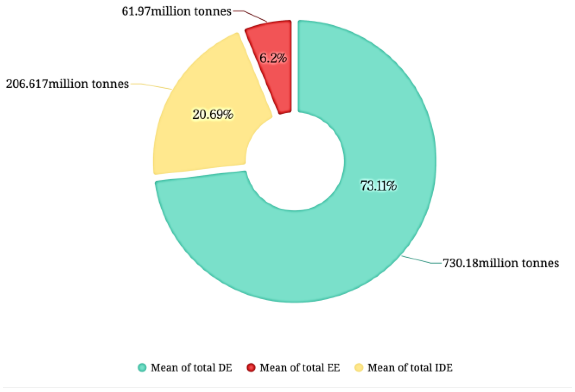
Figure 1 illustrates the trends of CS, CE, NCS and CBR for the 30 provinces as a whole from 2004 to 2019. During the sample period, NCS and CBR have three extremely pronounced peaks in 2008,2012 and 2015, with the maximum value during the sample period (1399.802million tonnes; 2.302) reached in 2015, with a significant net carbon effect. Overall, as the changes in CE are relatively stable, the trends in NCS and CBR are primarily influenced by changes in CS, which exhibit significant interannual variability, leading to a fluctuating upward trend. In 2015, CE reached their maximum value of 1075.088 million tons and then began to decrease slowly, indicating that the farming industry has the potential to absorb more carbon emissions generated by other industries. The composition of the CE is shown in Figure 2, with DE accounting for the largest proportion (73%). The main reason for the decreasing trend of CE is the gradual decrease of DE since 2013. It appears that the reduction in soil carbon emissions has played a significant role in this change, which shows that farming systems and methods have been improved and optimized to a considerable extent.

4.2. Empirical Results

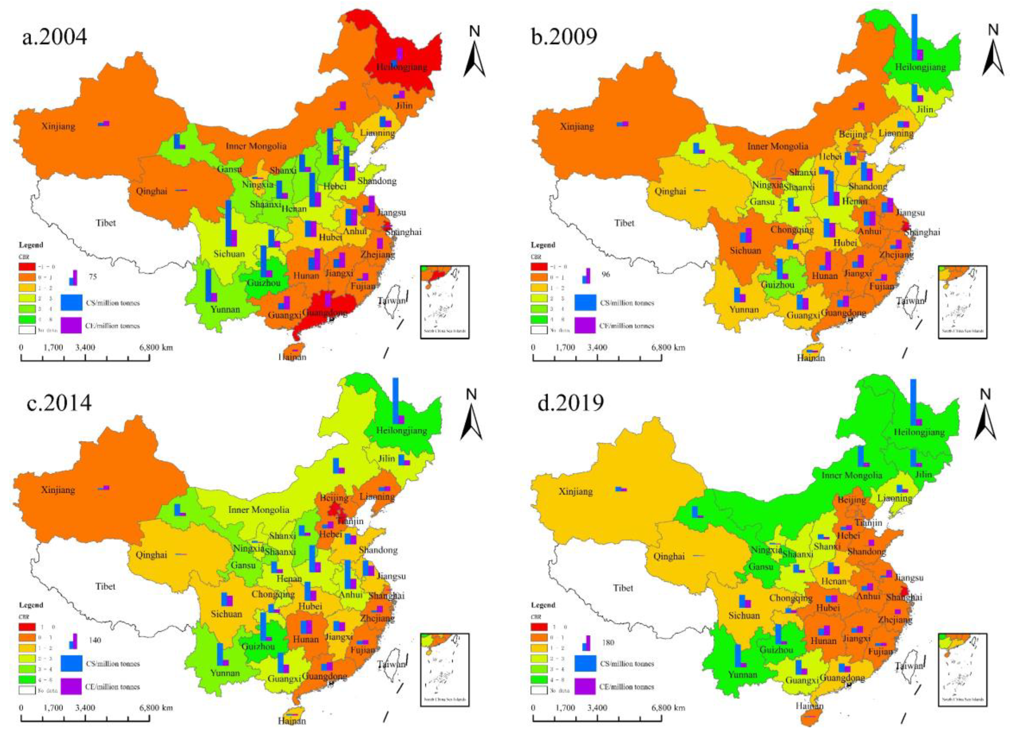
The Moran’s I test was conducted to determine the spatial correlation of CBR and the spatial correlation of lnSCALE from 2004-2019. As shown in Table 4, the results indicate that the explained variable CBR was found to be significant at a 5% level in all years except for 2009 which did not pass the test. Additionally, the core explanatory variable, CBR , passed the significance test of 1% in all years. These findings suggest that both CBR and lnSCALE have significant spatial correlation. Upon observing Figure 3, it becomes apparent that CBR displays a distinct pattern of “high-high” and “low-low” aggregation. As a result, it would be advisable to employ a spatial econometric model to examine the impact of land management scale expansion on emission reduction and sink enhancement.

4.2.1. Spatial Spillover Effects

The results of the OLS estimation in equation (4) and the FE estimation in equation (5) are presented in accordance with the econometric model design and the results of the relevant tests discussed in the previous section. After conducting the Hausman test, which suggests the use of the fixed effects model, the LR test shows that individual fixed effects should be used, and the results of the LM test, the LR test and the Wald test show that the SDM model should be used, and the SDM model has the highest goodness-of-fit, R2, in the estimation results, which is therefore suitable to be chosen as the final estimation results of the spatial models.
Table 5 shows the final estimation results of the corresponding coefficients of the individual models. Upon analysing the estimation results of the SDM model, it was found that the estimated value of the spatial autoregressive coefficient ρ is 0.467 and is significant at the 1% level, which suggest that the use of the spatial model in this paper is appropriate. There is a significant positive spatial correlation effect of CBR , the more neighbouring regions, the stronger the externality from the neighbouring regions, indicating that the carbon balance status of China’s farming industry shows obvious spatial clustering characteristics, and the carbon balance of this region is closely related to that of the neighbouring regions.
The regression coefficients suggest that most explanatory and control variables are significant, with the exception of lnSA , lnUCA , and SR . As for lnSACLE , lnINCOME , and lnEDU , their directions of coefficients are in line with the theoretical expectations presented in the previous section. Among the control variables, the coefficient of lnUCE is significantly positive at the 1% level, while the coefficient of lnUCA is insignificantly negative. This suggests that the yield of cash crops may not have a statistically significant effect on the carbon balance of farming. Even if it does, it may be negative. Additionally, the coefficient of LI is significantly negative. This indicates that while an increase in food production can be beneficial to carbon fixation and accumulation, the negative effects of increasing land use intensity may offset a part of the positive effects of increasing production. It has been observed that the coefficient of SR is positive, which is in line with previous studies that have suggested that returning straw to the field has a positive impact on the net carbon sink of agriculture. Additionally, it is worth noting that all three natural factors’ control variables are significant, which means that CBR is not solely an economic variable.
The spatial lag variable of the explanatory variables is an indicator that can effectively analyse whether there is a spatial relationship between the explained variables and the explanatory variables. According to Table 6, it can be observed that the spatial coefficient of lnSCALE is significantly positive, which implies that expanding the land management scale could have a positive spatial effect on the carbon balance of farming in neighbouring areas. Thus, further analysis based on the effect’s decomposition is necessary. Table 6 illustrates that lnSCALE has a noteworthy spatial spillover effect and total effect on CBR , which confirms hypothesis 1. The coefficients for the spatial spillover effect and the total effect are 4.508 and 5.750 respectively. Notably, the coefficient for the indirect effect (4.508) is larger than the coefficient for the direct effect (1.693), implying that the spatial spillover intensity of lnSCALE on CBR has an increasing trend.
It is widely acknowledged that expanding the scope of land management in farming operations can lead to improved technical efficiency, which can be achieved through the implementation of advanced agricultural technologies and practices, which can result in more effective resource management. As a result, this can contribute to the creation of increased carbon sinks and a reduction in carbon emissions. As these technologies and knowledge are shared between regions, neighbouring farmers may consider adopting these more environmentally friendly methods, which could contribute to improving the environmental performance of the region as a whole.
As an example, it can be noted that Zhejiang Province has achieved significant success in appropriately scaled agricultural operations, with positive effects spreading to neighbouring provinces [51]. Given its large population and limited land, it is necessary to develop multiple forms of appropriately scaled agricultural operations in Zhejiang to achieve agricultural modernisation. The province has implemented various measures and innovative practices to promote appropriately scaled agricultural operations, including land transfer and services for appropriate and compound operations. Additionally, the province places a high priority on environmentally friendly and ecologically sustainable agricultural production. The implementation of efficient and ecological farming systems and the construction of an efficient and ecological agricultural industry chain have been instrumental in promoting the development of agricultural production methods in a more environmentally friendly and sustainable direction. For example, improvements in farming systems, such as the integration of planting and breeding, and the combination of cereals with cash crops, have not only led to better use of land in terms of time and space, but also to more ecological and sustainable agricultural production. The model of appropriately scaled agricultural operation, as implemented in Zhejiang Province, has been gradually adopted by neighbouring provinces, such as Jiangsu and Shanghai, through various forms of exchange activities, policy promotion, and demonstration. While learning from and incorporating the experience of Zhejiang, these regions have also made localized innovations and improvements based on their own unique situations. These efforts have collectively enhanced the benefits of regional agricultural carbon sinks and emission reduction, effectively promoting the greening and modernization of agricultural production [52].
The indirect effect of lnEDU , while not significant, is still worth discussing due to its direction being opposite to the direct effect and its absolute magnitude being comparable to that of the direct effect. One possible explanation for this phenomenon is that human capital in rural areas may have a positive impact on the income of farmers within the same province, but a notably negative impact on the income of farmers in neighbouring provinces, suggesting a clear spatial competition effect [53]. Therefore, in the western region of China, farmers with lower levels of education and training face significant competition from labour forces in other provinces. As a result, they have opted to cultivate more non-grain crops in order to increase their income. This has led to a more pronounced spatial “non grain” (the use of arable land for non-grain purposes) pattern from the northeast to the southwest [54]. Cash crop production may not contribute to improving carbon sequestration and reducing agricultural emissions, and may even be detrimental. Thus, it is possible that alterations to the cropping structure of nearby rural areas with higher levels of education may have an indirect impact on the effectiveness of the region’s farming with regards to carbon sinks and emission reductions.
To ensure the robustness of the spatial measurements, the same regression of equation (9) was performed after replacing the spatial adjacency matrix with a spatial distance matrix (refer to Table 7). Comparison of the results indicates that, with the exception of a slight modification in the size of the impact coefficients, the direction and significance of the impacts remain consistent with the model (5) in Table 5.This highlights the robustness of the empirical findings.

4.2.2. Threshold Characteristics

The existence of the threshold effect was first tested, and the F-values corresponding to the single-threshold model rejected the original hypothesis at the 5% level, but the double-threshold model failed to reject the original hypothesis. According to the results of the significance level test, it can be concluded that there is a single threshold effect on the impact of rural residents’ income level and education level on the carbon balance of farming in the context of changes in land management scale. As a result, hypothesis 2 is confirmed.
The estimation results of model (1) in Table 8 indicate that when lnSCALE is below the threshold value of 0.594, the coefficient estimate of lnINCOME is -1.116, which implies that the income level of rural residents has a negative effect on the carbon balance of agriculture at this stage; when lnSCALE is greater than 0.594, the coefficient estimate of lnINCOME is 1.259, indicating that with the expansion of the scale of land management, the effect of income level on the carbon balance turns from negative to positive. It has been proven that the “U-shaped” curve of income and carbon balance is valid, and that after a certain size of area per labourer, the agricultural production and management mode of farmers begins to change from the traditional factor-driven production mode to the environmentally friendly green production mode.
The findings of Guan et al. (2023) [11] are supported by the threshold model outlined in this paper. Moreover, it is observed that as the land management scale increases, the effect of lnEDU on CBR shifts from positive to negative once the lnSCALE surpasses the threshold, resulting in an “inverted U-shaped” pattern of the association. To further explore the factors contributing to the formation of the “inverted U-shaped” curve, we conducted a thorough analysis of the CBR by replacing the explained variables with CE and CS, and decomposed CS into carbon sinks per unit of sown area (UCS) and SA, applying a regression of the threshold panel model. The findings of this analysis are presented in Table 8, model (2) (3) (4). According to the estimation results, it appears that a considerable proportion of the threshold characteristics of lnEDU on CBR are attributed to lnSA . Moreover, it seems that the impact of lnEDU on lnSA is not significant until lnSCALE reaches the threshold; After the land management scale reaches a certain level, it has been observed that the effect of lnEDU on lnSA becomes significantly negative. This suggests that an increase in the average level of education of rural residents by 1% will lead to a reduction of 1.526% in the total sown area of crops. This finding is consistent with the research conducted by Zhou. (2009) [55].
In summary, a possible inference is that: (i) the increasing/decreasing effect of INCOME/EDU on CE diminishes at the margin as scale increases; (ii) at the same time, the negative effect of INCOME/EDU on SA changes from an insignificant weak negative effect to a significant positive effect/from an insignificant weak positive effect to a significant negative effect after crossing the threshold (0.007); (iii) The decreasing marginal effect in (i) is difficult to gradually offset and neutralise the reverse change of the effect in (ii), which ultimately leads to the reverse change of INCOME/EDU on CBR at the threshold (0.594) in the same direction as in (ii). This explains the formation mechanism of the “U-shaped”/“inverted U-shaped” curve that characterises INCOME/EDU and CBR.

5. Further Discussion

5.1. Analysis of Spatial Heterogeneity

Further sub-regional analysis is discussed in this paper, given the wide variation across China’s geographical sub-regions. The 30 provinces have been categorized into four major economic regions, namely Northeast, East, Central and West, as developed by the National Bureau of Statistics of China. To represent the region and land management scale, three interaction term variables have been generated.
nlnSCALE it = (   lnSCALE it   -   lnSCALE it ¯   )   ×   northeast
elnSCALE it = (   lnSCALE it   -   lnSCALE it   ¯ )   ×   east
wlnSCALE it = (   lnSCALE it   -   lnSCALE it   ¯ )   ×   west
In the above equation, northeast , east and west are dummy variables representing the corresponding regions, taking the value 1 if the province in which the observation is located is in the corresponding region and 0 otherwise. lnSCALE ¯ is the mean of lnSCALE , for which centring avoids multicollinearity between variables.
The results presented in Table 9 were derived by performing a regression analysis on the three interaction variables in equation (9), with the coefficient of nlnSCALE being 10.833. At a 1% significance level, the result indicates that expanding land management scale in the Northeast region is more effective in reducing carbon emissions and increasing carbon sinks from farming industry compared to the non-Northeast region. Moreover, the coefficient of elnSCALE is significantly negative, indicating that expanding land management scale in the East region has a limited effect on the carbon balance of the farming industry. In contrast, the insignificant result of wlnSCALE suggests that the western region may have less spatial heterogeneity compared to other regions.
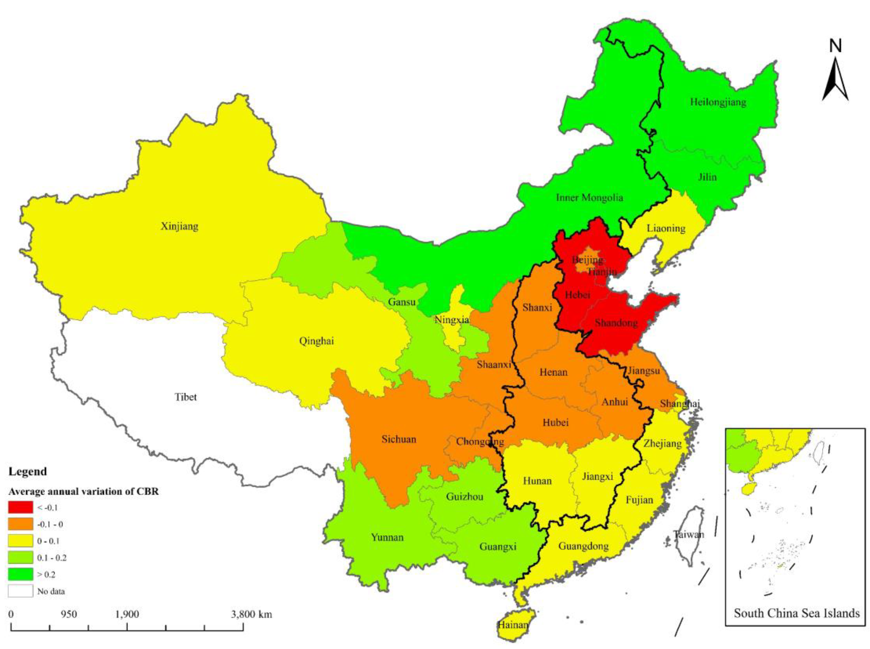
There appears to be a significant spatial heterogeneity between the Northeast and non-Northeast regions, as indicated by the coefficients. As shown in Figure 4, the spatial heterogeneity between Northeast and non-Northeast regions is reflected in the fact that the provinces with an average annual variation of CBR>0.2 are Heilongjiang (0.51), Jilin (0.26) in the Northeast, and Inner Mongolia (0.31). Their mean SCALE in the sample period is great than 1.4 hectare·person-1, which is much larger than the mean of SCALE (0.55 hectare·person-1) in China. This difference can be attributed to the distinct agricultural production practices in the Northeast and non-Northeast regions. The Northeast region has a highly mechanised agricultural production system that emphasises technological advancements, which is in contrast to the smallholder economy style of agricultural production in China’s traditional core regions [56]. Moreover, The Northeast Plain of China boasts a vast black soil belt, which can be compared to the plains of Eastern Europe and the Great Plains of the United States. By expanding the scale of land management and promoting the scientific rationalisation of farming systems, the carbon sequestration capacity of this fertile land can be greatly stimulated [57]. Although the mean of SCALE in Ningxia and Xinjiang, located in the Northwest region, is also above 1 hectare·person-1, the average annual variation of CBR did not increase significantly during the sample period due to agricultural constraints imposed by natural endowments.

5.2. Threshold Value

Section 4.2.2 presents an estimate of 0.594 as the threshold value of the variable l n S C A L E in the threshold panel model. It is worth noting that only 6.25% of the sample exceeds this threshold, and these observations belong to only 1/10th of the total number of regions (which are still limited to the three provinces of Heilongjiang, Jilin, and Inner Mongolia). In practical terms, it could be argued that the threshold value is approximately 1.81 hectare·person-1, which is significantly higher than the average of 0.55 hectare·person-1 observed during the Chinese sample period. If the national average land management scale were to reach this threshold level, it could potentially result in a reduction of the rural labour force by at least two-thirds more to achieve this, which is due to the fact that the area of arable land is roughly stable. This suggests that over a long period of time, most provinces would remain stable on the left side of the threshold. At this stage, INCOME has a negative impact on the CBR, while EDU has a positive impact on the CBR. The data shows that the average annual growth rate of lnINCOME / lnEDU across China’s provinces during the 2004-2019 period was 7.47‰ per year/3.02‰ per year. Based on the estimation in Table 8, it can be inferred that the CBR would experience an average annual impact of -0.83%/1.71%. In other words, the negative effect of INCOME at this stage can be fully offset by the positive effect of EDU, and overall, the development of China’s rural economic and social levels is unlikely to worsen the net carbon effect of farming in the short term.
In the Northeast, the extent of land management in agriculture has exceeded the threshold value. The factors driving this expansion exhibit similarities with other regions, as well as distinct reasons of their own. Since the 1990s, the population of the north-eastern region has been decreasing due to various factors, such as the inflexibility of the economic system and the depletion of resources. It is worth noting that from 2010 to 2020, the population of the North-East decreased by 10%, which is equivalent to the population of Belgium. As a result of the current situation, farmers in the northeast who possess adequate human capital are leaving the region in large numbers. Meanwhile, local farmers who continue to engage in agricultural production may inevitably increase their use of high-carbon agricultural materials, who may also adopt less rational production methods and farming systems to replace the rapidly diminishing agricultural labour force in the short term [58]. The higher the level of education of the rural population, the greater the willingness of farmers to migrate to other sectors or even to other regions, and the more likely it is that the carbon balance of agriculture will be negatively affected in the short term.

6. Conclusion

This study employs a novel accounting method to evaluate the net carbon effect of the farming industry, building on previous academic research. By examining data from 30 provinces in China from 2004 to 2019, using spatial panel regression models and threshold panel regression models, this paper aims to reveal the spatial correlation between land management scale and carbon balance ratio, as well as the non-linear characteristics between carbon balance ratio and income level of rural residents and education level of rural residents. The results indicate the following:
(1) During the study period, it was found that most regions of China demonstrated a net sink effect of the farming industry. The national net carbon sink of the farming industry showed fluctuating growth, indicating that it plays a positive role in providing carbon emission absorption space for other high-carbon emitting industries, which contribution is significant in achieving the national carbon peak and carbon neutrality goals.
(2) The findings of the spatial panel model indicate that the scale of land management has a positive spatial spillover effect on the carbon balance, which is significant and varies spatially. Notably, the expansion of land management in the northeast region has a particularly significant impact on increasing sinks and reducing emissions in the farming industry.
(3) According to the threshold panel model analysis, it can be inferred that the impact of rural residents’ income and education levels on the carbon balance of the farming industry will change in the opposite direction as the scale of land management expands. However, this threshold has not yet been reached in most regions. As a result, it can be generally concluded that an increase in income level will lead to a decrease in the net sink effect of farming, while an increase in education level will enhance the effect.
This study proposes the following policy recommendations based on the research results: Firstly, it is suggested that the development of a unified carbon accounting system be expedited, and a scientific and reasonable accounting scope and methodology be established. Secondly, it is recommended that appropriately scaled agricultural operations be continued to be promoted, and that large-scale agricultural operations be incentivised and supported. It is also suggested that the combination of agricultural production factors be rationally deployed, and that institutional mechanisms that hinder the transfer of land be gradually eliminated. This will help accelerate the process of large-scale and industrialised agriculture. In addition to improving farmers’ income, it is important to also recognize the intangible value of human capital, promote the development of new types of agribusinesses, enhance the cultural quality and vocational ability of farmers, raise awareness and provide guidance on the concept of green agricultural production, and offer practical economic and material support to facilitate the transition from traditional modes of agricultural operation. Finally, it is suggested that carbon functional regions be established on a pilot basis. Regions with high carbon emissions should be provided with material and economic compensation, while ecological resources should be directed towards high carbon sink regions through transfer payments. This will allow for the full utilization of their carbon and ecological carrying advantages, while also ensuring national food security and ecological safety.

Author Contributions

Conceptualization, W.W. and J.G.; methodology, W.W.; software, W.W. and Y.C; validation, W.W.; resources, W.W. and J.G; data curation, W.W., Y.C., Y.G., A.G. and H.W.; writing—original draft preparation, W.W.; writing—review and editing, W.W. and J.G; visualization, Y.C., Y.G. and A.G.; supervision, W.W.; project administration, W.W.; funding acquisition, W.W. and J.G. All authors have read and agreed to the published version of the manuscript.

Funding

This research was supported by the Innovation and Entrepreneurship Training Program at Northeast Forestry University (DC-2024177); the Outstanding Youth Project of Natural Science Foundation of Heilongjiang Province (YQ2019G001); Fundamental Research Funds for the Central Universities of China (2572021BM02); the Research Projects of Humanities and Social Sciences Foundation of Ministry of Education of China (23YJC790036).

Institutional Review Board Statement

Not applicable.

Informed Consent Statement

Not applicable.

Data Availability Statement

The data presented in this study are available upon request from the corresponding author.

Conflicts of Interest

The authors declare no conflict of interest.

References

  1. Lee, H.; Calvin, K.; Dasgupta, D.; Krinner, G.; Mukherji, A.; Thorne, P.; Trisos, C.; Romero, J.; Aldunce, P.; Barrett, K. Climate change 2023: synthesis report. Contribution of working groups I, II and III to the sixth assessment report of the intergovernmental panel on climate change; The Australian National University: Canberra, Australia, 2023. [Google Scholar]
  2. Rogelj, J.; Popp, A.; Calvin, K. V.; Luderer, G.; Emmerling, J.; Gernaat, D.; Fujimori, S.; Strefler, J.; Hasegawa, T.; Marangoni, G. Scenarios towards limiting global mean temperature increase below 1.5 C. Nature climate change 2018, 8, 325–332. [Google Scholar] [CrossRef]
  3. Keenan, T.F.; Williams, C.A. The terrestrial carbon sink. Annual Review of Environment and Resources 2018, 43, 219–243. [Google Scholar] [CrossRef]
  4. Lynch, J.; Cain, M.; Frame, D.; Pierrehumbert, R. Agriculture’s contribution to climate change and role in mitigation is distinct from predominantly fossil CO2-emitting sectors. Frontiers in sustainable food systems 2021, 4, 518039. [Google Scholar] [CrossRef] [PubMed]
  5. Zhao, M.; Shi, R.; Du, R.; Yao, L. The pathway to China’s carbon–neutral agriculture: Measures, potential and future strategies. Chinese Political Science Review 2023, 8, 304–324. [Google Scholar] [CrossRef]
  6. Johnson, J.M.F.; Franzluebbers, A.J.; Weyers, S.L.; Reicosky, D.C. Agricultural opportunities to mitigate greenhouse gas emissions. Environmental pollution 2007, 150, 107–124. [Google Scholar] [CrossRef] [PubMed]
  7. Tian, Y.; Zhang, J. Regional Differentiation Research on Net Carbon Effect of Agricultural Production in China. Journal of Natural Resources 2013, 28, 1298–1309. [Google Scholar]
  8. Chen, L.; Xue, L.; Xue, Y. Spatial Agglomeration and Variation of China’s Agricultural Net Carbon Sink. Ecology and Environmental Sciences 2015, 24, 1777–1784. [Google Scholar]
  9. Shang, J.; Yang, B. Estimation of Carbon Source and Carbon Sequestration in Planting Industry and Dynamic Analysis of Influencing Factors of Net Carbon Sequestration: A Case Study of Shandong Province. Reform 2019, 2019, 123–134. [Google Scholar]
  10. Li, B.; Wang, C.; Zhang, J. Dynamic evolution and spatial spillover of China’s agricultural net carbon sink. China Population, Resources and Environment 2019, 29, 68–76. [Google Scholar]
  11. Guan, J.; Zhang, S.; Ren, Y.; Sheng, C. Random forest model-assisted evaluation of spatiotemporal differentiation of China’s agricultural net carbon sink and evolution of influencing factors. China Environmental Science 2024, 44, 1158–1170. [Google Scholar]
  12. Wu, H.; Meng, Y.; Huang, H.; Chen, W. Spatiotemporal Coupling Between the Net Carbon Sequestration of Cropland Use and Agricultural Production in China. Journal of Soil and Water Conservation 2022, 36, 360-368+376. [Google Scholar]
  13. Lu, J.; Huang, X.; Dai, L.; Chen, Z.; Li, Y. Spatio-temporal Scale Analysis on the Equality of Energy Consumption Carbon Emission Distribution in China. Journal of Natural Resources. 2012, 27, 2006–2017. [Google Scholar]
  14. Du, J.; Luo, J.; Wang, R.; Wang, X. The Estimation and Analysis of Spatio-Temporal Change Patterns of Carbon Functions in Major Grain Producing Area. Journal of Ecology and Rural Environment 2019, 35, 1242–1251. [Google Scholar]
  15. Yang, Y.; Shi, Y.; Sun, W.; Chang, J.; Zhu, J.; Chen, L.; Wang, X.; Guo, Y.; Zhang, H.; Yu, L.; et al. Terrestrial carbon sinks in China and around the world and their contribution to carbon neutrality. Science China Life Sciences 2022, 65, 861–895. [Google Scholar] [CrossRef] [PubMed]
  16. Lund, P.J.; Hill, P.G. Farm size, efficiency and economies of size. Journal of Agricultural Economics 1979, 30, 145–158. [Google Scholar] [CrossRef]
  17. Luo, B.; Zhou, J.; Zang, H.; Sawut, A.; Feng, X.; Yang, Y.; Peixoto, L.; Wang, X.; Olesen, J.E.; Zeng, Z. Optimize farm size and agronomic practices to improve agricultural sustainability: a case of multi-indicator assessment from the North China Plain. Environment, Development and Sustainability 2023, 1–20. [Google Scholar] [CrossRef]
  18. Zhang, X. Study on Farm Size and Smallhoders Productivity in China; Chinese Academy of Agricultural Sciences, 2018. [Google Scholar]
  19. Xiao, X.; Li, Q. Agricultural production: accumulation of science and technology and the spatial spillover-a research based on the spatial panel data between 1986-2010. China Economic Studies 2013, 2013, 43–50. [Google Scholar]
  20. Gu, N.; Zhang, T. Financial Inclusion Development and Rural Poverty Reduction: Threshold, Spatial Spillover and Channel Effect. Journal of Agrotechnical Economics 2019, 74–91. [Google Scholar]
  21. Campi, M.; Duenas, M.; Fagiolo, G. How do countries specialize in agricultural production? A complex network analysis of the global agricultural product space. Environmental Research Letters 2020, 15, 124006. [Google Scholar] [CrossRef]
  22. Yao, H.; Zhao, X.; Gao, Q. Knowledge Flow and Spatial Interaction of Agricultural Science and Technologyamong Provinces in China. Science & Technology Progress and Policy 2021, 38, 34–42. [Google Scholar]
  23. Wang, Y.; Di, F.; Xin, L. The status and Problems of Grain Production in the Main Grain production Areas of China and Policy Suggestions. Research of Agricultural Modernization 2018, 39, 37–47. [Google Scholar] [CrossRef]
  24. Zhang, L.; Luo, B. Agricultural Reduction: the Logic of Scale in Agriculture and Its Evidence. Issues in Agricultural Economy 2020, 81–99. [Google Scholar]
  25. Wei, M.; Yan, T.; Luo, S. Impacts of Scale Operation and Technological Progress on Green and Low-carbon Development of Agriculture: a Quasi-natural Experiment Based on the Establishment of Major Grain-producing Areas. Issues in Agricultural Economy 2023, 41–65. [Google Scholar]
  26. Grossman, G.M.; Krueger, A.B. Environmental impacts of a North American free trade agreement. 1991. [Google Scholar]
  27. Grossman, G.M.; Krueger, A.B. Economic growth and the environment. The quarterly journal of economics 1995, 110, 353–377. [Google Scholar] [CrossRef]
  28. Schultz, T.W. Transforming traditional agriculture: Reply. Journal of farm Economics 1966, 48, 1015–1018. [Google Scholar] [CrossRef]
  29. Gu, B.; Duan, J.; Ren, C.; Wang, S.; Wang, C. Large-scale farming promotes agricultural green development in China. Journal of Agricultural Resources and Environment 2021, 38, 709–715. [Google Scholar]
  30. Drahmoune, F. Agrarian transitions, rural resistance and peasant politics in Southeast Asia. Journal of Current Southeast Asian Affairs 2013, 32, 111–139. [Google Scholar] [CrossRef]
  31. Liu, Q.; Xiao, H. What is the logic of the scale of farm management that affects agricultural carbon emissions? The mediating role of factor inputs and the moderating role of cultural quality. Rural Economy 2020, 10–17. [Google Scholar]
  32. Woodwell, G.M.; Whittaker, R.H.; Reiners, W.A.; Likens, G.E.; Delwiche, C.C.; Botkin, D.B. The Biota and the World Carbon Budget: The terrestrial biomass appears to be a net source of carbon dioxide for the atmosphere. Science 1978, 199, 141–146. [Google Scholar] [CrossRef]
  33. Hu, Y.; Zhang, K.; Hu, N.; Wu, L. Review on measurement of agricultural carbon emission in China. Chinese Journal of Eco-Agriculture 2023, 31, 163–176. [Google Scholar]
  34. IPCC. Climate change 2022: mitigation of climate change; Cambridge University Press: Cambridge, UK; New York, NY, USA, 2022. [Google Scholar]
  35. Fan, Z.; Song, C.; Qi, X.; Wu, F. Accounting of greenhouse gas emissions from China’s agricultural system in recent 40 years. Acta Ecologica Sinica 2022, 42, 9470–9482. [Google Scholar]
  36. Zhang, G.; Lu, F.; Huang, Z.; Chen, S.; Wang, X. Estimations of application dosage and greenhouse gas emission of chemical pesticides in staple crops in China. Chinese Journal of Applied Ecology 2016, 27, 2875–2883. [Google Scholar]
  37. Lal, R. Carbon emission from farm operations. Environment international 2004, 30, 981–990. [Google Scholar] [CrossRef] [PubMed]
  38. Feng, Z.; Liu, B.; Yang, Y. A Study of the Changing Trend of Chinese Cultivated Land Amount and Data Reconstructing: 1949-2003. Journal of Natural Resources 2005, 2005, 35–43. [Google Scholar]
  39. Bi, Y.; Zheng, Z. THE ACTUAL CHANGES OF CULTIVATED AREA SINCE THE FOUNDING OF NEW CHINA. Resources Science 2000, 2000, 8–12. [Google Scholar]
  40. Wang, Y.; Wang, B.; Ma, C.; Zhong, X.; Cai, Y. Study on the Multiple Cropping Index Based on Revised Cultivated Land Area in China. China Land Science 2008, 22, 46–52. [Google Scholar]
  41. Chen, Z.; Lu, M.; Jin, Y. Regional Differences of Human Capitals and Education Development in China: An Estimation of the Panel Data. The Journal of World Economy 2004, 2004, 25-31+77. [Google Scholar]
  42. Devendra, C.; Thomas, D. Smallholder farming systems in Asia. Agricultural systems 2002, 71, 17–25. [Google Scholar] [CrossRef]
  43. Zuo, L.; Zhang, Z.; Dong, T. Progress in the Research on the Multiple Cropping Index. Journal of Natural Resources 2009, 24, 553–560. [Google Scholar]
  44. Fan, J.; Wu, B. A Study on Cropping Index Potential Based on GIS. Journal of Remote Sensing 2004, 637–644. [Google Scholar]
  45. Li, Y.; Xue, C.; Chai, C.; Yao, S.; Li, W. Spatio-temporal variation and driving forces of net carbon sink of conservation tillage in China. China Population, Resources and Environment 2022, 32, 15–23. [Google Scholar]
  46. He, Q.; Ju, W.; Dai, S.; He, W.; Song, L.; Wang, S.; Mao, G. Drought risk of global terrestrial gross primary productivity over the last 40 years detected by a remote sensing-driven process model. Journal of Geophysical Research: Biogeosciences 2021, 126, e2020JG005944. [Google Scholar] [CrossRef]
  47. Muntean, M.; Janssens-Maenhout, G.; Song, S.; Giang, A.; Selin, E.N.; Zhong, H.; Zhao, Y.; Olivier, J.G.J.; Guizzardi, D.; Crippa, M.; et al. Evaluating EDGARv4.tox2 speciated mercury emissions ex-post scenarios and their impacts on modelled global and regional wet deposition patterns. Atmospheric Environment 2018, 184, 56–68. [Google Scholar] [CrossRef]
  48. Shan, Y.; Guan, D.; Zheng, H.; Ou, J.; Li, Y.; Meng, J.; Mi, Z.; Liu, Z.; Zhang, Q. China CO2 emission accounts 1997-2015. Scientific data 2018, 5, 1–14. [Google Scholar] [CrossRef] [PubMed]
  49. Elhorst, J.P. Spatial panel data models. Spatial econometrics: From cross-sectional data to spatial panels 2014, 37–93. [Google Scholar]
  50. Hansen, B.E. Threshold effects in non-dynamic panels: Estimation, testing, and inference. Journal of econometrics 1999, 93, 345–368. [Google Scholar] [CrossRef]
  51. Li, H.; Fu, L.; Huang, Z.; Peng, W. Various forms of moderate-scale management of agriculture and development prospects. Acta Agriculturae Zhejiangensis 2021, 33, 161–169. [Google Scholar]
  52. Ye, B. Status Quo and Countermeasures for Green Development of Zhejiang Agriculture. Journal of Zhejiang Agricultural Sciences 2022, 63, 1434–1436. [Google Scholar]
  53. Luo, L.; Fan, L. Spatial Characteristics of Income-Enhancing Effects of Rural Human Capital in China. Journal of Management World 2014, 2014, 58–76. [Google Scholar]
  54. Meng, F.; Tan, Y.; Chen, H.; Xiong, W. Spatial-temporal Evolution Patterns and Influencing Factors of “Non-grain” Utilization of Cultivated Land in China. China Land Science 2022, 36, 97–106. [Google Scholar]
  55. Zhou, Q. Analysis of Factors Affecting Farmers’ Willingness to Grow Food. Journal of Agrotechnical Economics 2009, 2009, 25–30. [Google Scholar]
  56. He, X. Reflections on the scale of land management in agriculture in China. Issues in Agricultural Economy 2016, 37, 4–15. [Google Scholar]
  57. Yu, Y.; Huang, Y.; Zhang, W. Projected changes in soil organic carbon stocks of China’s croplands under different agricultural managements, 2011–2050. Agriculture, ecosystems & environment 2013, 178, 109–120. [Google Scholar]
  58. Liu, F. A Study of the Conditions of the Scale Operation of Farmland, and of the Effect thereof: Taking the Northeastern Countryside as a Case. Journal of Management World 2006, 2006, 71-79,171-172. [Google Scholar]
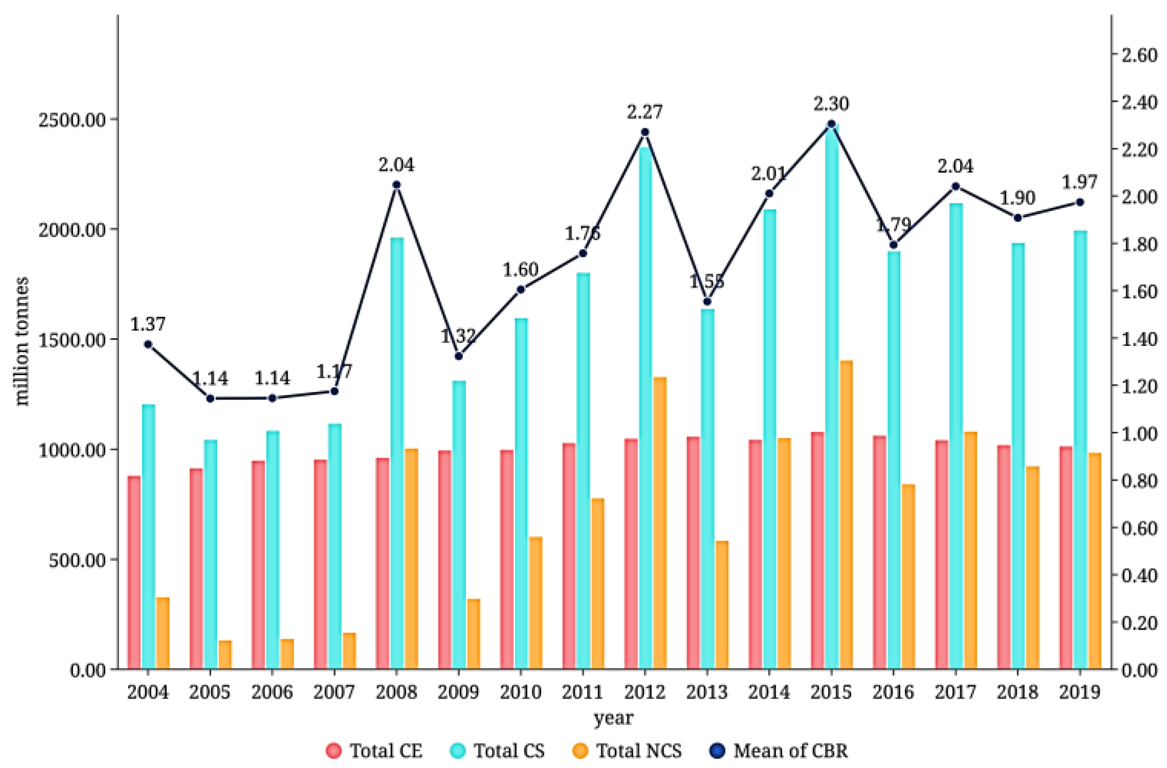
Figure 1. CBR trends in China (2004-2019). Notes: Mean of CBR = Total CS / Total CE.
Preprints 104350 g001
Figure 2. Composition of CE in China on average over the sample period.
Preprints 104350 g002
Figure 3. Spatial distribution of CBR in farming (2004, 2009,2014 and 2019).
Preprints 104350 g003
Figure 4. Spatial distribution of average annual variation in CBR.
Preprints 104350 g004
Table 1. Carbon emission factors of agricultural inputs.
Carbon emissions source Emission factor Data source
Nitrogen fertilizer production, transportation and use 1.53 kg(CO2)·kg−1 [35]
Phosphate fertilizer production, transportation and use 1.63 kg(CO2)·kg−1 [35]
Potassium fertilizer production, transportation and use 0.65 kg(CO2)·kg−1 [35]
Compound fertilizer production, transportation and use 1.77 kg(CO2)·kg−1 [35]
Pesticide production, transportation and use 4.9341 kg(C)·kg−1 [36]
Agricultural plastic film production, transportation and use 5.18 kg(C)·kg−1 [37]
Table 2. GWP100 values.
Gas AR6-GWP100 Lifetime
CO2 1 N/A
CH4 27 11.8
N2O 273 109
Table 3. Decriptive statistics.
Variables Unit Observations Mean Standard deviation Min Max
SCALE hectare·person-1 480 0.701 0.578 0.192 3.524
INCOME yuan 480 9975 5450 2638 33195
EDU year 480 8.421 0.877 5.368 11.50
SA 1000 hectares 480 5371 3643 88.60 14783
UCE kg·hectare-1 480 5130 1016 2870 8169
UCA kg·hectare-1 480 7702 5899 1159 33608
LI 480 0.646 0.144 0.343 0.982
SR 480 0.191 0.164 0 0.680
TEM °C 480 13.93 5.328 2.549 25.43
SUN hour 480 2047 485.9 933.0 2960
PRE mm 480 953.1 447.3 200.8 2232
Table 4. Global Moran index.
year CBR lnSCALE
Moran’s I Z value P value Moran’s I Z value P value
2004 0.4273 3.6710 0.0002 0.6973 5.9634 0.0000
2005 0.4051 3.5236 0.0004 0.7039 6.0274 0.0000
2006 0.2966 2.6500 0.0080 0.7082 6.0796 0.0000
2007 0.3998 3.5533 0.0004 0.7015 6.0500 0.0000
2008 0.3277 2.9128 0.0036 0.7293 6.2985 0.0000
2009 0.1313 1.3591 0.1741 0.7132 6.1818 0.0000
2010 0.3557 3.2597 0.0011 0.7070 6.1350 0.0000
2011 0.3219 2.9218 0.0035 0.7017 6.0893 0.0000
2012 0.3571 3.2271 0.0013 0.7052 6.1379 0.0000
2013 0.4528 3.8892 0.0001 0.6886 5.9876 0.0000
2014 0.2827 2.6566 0.0079 0.6722 5.8556 0.0000
2015 0.2426 2.3379 0.0194 0.6539 5.7066 0.0000
2016 0.2970 2.7253 0.0064 0.6472 5.6286 0.0000
2017 0.3545 3.3022 0.0010 0.6305 5.4774 0.0000
2018 0.4103 3.6126 0.0003 0.6249 5.4032 0.0000
2019 0.4953 4.3207 0.0000 0.6182 5.3276 0.0000
Table 5. Spatial econometric results.
Variables (1) OLS (2) FE (3) SAR (4) SEM (5) SDM
CBR CBR CBR CBR CBR
lnSCALE 0.773** 1.495** 1.447** 1.213* 1.345**
(2.23) (2.22) (2.06) (1.76) (2.05)
lnINCOME 0.436 -2.370* -1.115*** -0.873** -3.108**
(1.18) (-1.76) (-3.71) (-2.46) (-2.39)
lnEDU -2.002 4.581 4.140* 4.820* 4.996**
(-1.08) (1.62) (1.92) (1.94) (2.06)
lnSA 0.399*** 2.462** 1.423* 1.248 1.308
(4.43) (2.62) (1.70) (1.38) (1.57)
lnUCE -3.118*** 5.075*** 4.575*** 4.358*** 4.051***
(-3.03) (3.81) (3.58) (2.85) (3.29)
lnUCA 0.596** -0.734 -0.438 -0.281 -0.249
(2.53) (-1.61) (-1.14) (-0.68) (-0.70)
LI -3.426** -3.924** -3.366*** -3.748*** -2.785*
(-2.32) (-2.29) (-2.83) (-2.72) (-1.69)
SR 1.834 1.456 0.290 0.441 1.129
(1.20) (1.29) (0.35) (0.49) (1.52)
lnPRE -0.232 2.287*** 1.277*** 1.980*** 2.279***
(-0.67) (4.26) (3.90) (4.10) (3.53)
lnTEM -0.599 -2.572*** -1.545** -1.801** -2.333***
(-1.18) (-2.82) (-2.37) (-2.27) (-2.99)
lnSUN -2.628** -1.228 -1.355*** -2.427** -2.036*
(-2.28) (-1.44) (-2.58) (-2.46) (-1.80)
Constant 43.618*** -42.929**
(2.85) (-2.15)
ρ 0.469*** 0.467***
(8.03) (8.56)
σ 0.540***
(9.83)
Observations 480 480 480 480 480
R2 0.433 0.470 0.406 0.389 0.497
ID FE YES YES YES YES
YEAR FE YES
Notes: Robust t-statistics/z-statistics in parentheses; *** p<0.01, ** p<0.05, * p<0.1.
Table 6. The direct and indirect effect decomposition of SDM.
Variables Wx Direct effect Indirect effect Total effect
lnSCALE 1.676* 1.693** 4.058** 5.750***
(1.76) (2.35) (2.44) (2.77)
lnINCOME 2.156 -3.062*** 1.253 -1.810***
(1.50) (-2.65) (0.90) (-2.92)
lnEDU -4.924 4.918** -4.562 0.356
(-1.47) (2.20) (-0.94) (0.07)
lnSA 1.213 1.575* 3.139** 4.714***
(1.18) (1.95) (2.05) (2.58)
lnUCE 0.057 4.317*** 3.332 7.649***
(0.03) (3.85) (1.43) (3.21)
lnUCA -0.791 -0.368 -1.587 -1.955
(-0.90) (-1.15) (-1.24) (-1.54)
LI 0.634 -2.947* -1.185 -4.131
(0.32) (-1.86) (-0.43) (-1.43)
SR 1.911 1.426* 4.171 5.598*
(1.29) (1.85) (1.63) (1.91)
lnPRE -1.811** 2.228*** -1.363* 0.865*
(-2.48) (3.87) (-1.70) (1.79)
lnTEM 0.859 -2.375*** -0.477 -2.852*
(0.77) (-3.18) (-0.31) (-1.96)
lnSUN 2.049 -1.901* 1.917 0.016
(1.42) (-1.92) (1.18) (0.02)
Notes: Robust z-statistics in parentheses; *** p<0.01, ** p<0.05, * p<0.1.
Table 7. Results after replacing the spatial matrix.
Variables Main Wx
lnSCALE 1.964*** 7.584***
(2.89) (4.39)
lnINCOME -3.107** 0.622
(-2.42) (0.45)
lnEDU 3.134 -9.833
(1.25) (-1.17)
lnSA 2.237** 5.422**
(2.56) (2.57)
lnUCE 5.402*** 2.117
(4.56) (0.51)
lnUCA -0.472 -1.268
(-1.17) (-1.16)
LI -2.964* 4.061
(-1.85) (0.85)
SR 1.861* 11.958***
(1.74) (2.68)
lnPRE 2.060*** -1.895**
(3.59) (-2.17)
lnTEM -2.748*** 5.054**
(-2.77) (2.48)
lnSUN -1.436* 1.862
(-1.65) (1.15)
Note: Same as table 6.
Table 8. The estimation results of panel threshold regression model.
Variables (1) (2) (3) (4)
CBR CE UCS lnSA
lnSCALE 1.780*** -1.136 3.536*** 0.101**
(4.38) (-1.20) (5.21) (2.41)
lnINCOME (lnscale≤δ1) -1.116*** 4.733*** -1.171*** -0.017
(-5.03) (6.59) (-3.32) (-0.75)
lnINCOME (δ1<lnscale≤δ2) 1.259** 2.414*** -1.513*** 0.334***
(2.36) (4.84) (-3.19) (8.91)
lnEDU (lnscale≤δ1) 5.665*** -13.309*** 5.953** 0.056
(3.64) (-3.29) (2.42) (0.34)
lnEDU (δ1<lnscale≤δ2) -3.927* -2.853 6.676** -1.526***
(-1.66) (-0.85) (2.51) (-8.09)
lnSA 1.534*** 7.821*** 0.089
(3.56) (8.72) (0.13)
lnUCE 4.632*** 7.658*** 8.562*** -0.360***
(6.75) (5.60) (8.53) (-5.15)
lnUCA -0.647*** 0.007 -0.877*** 0.066***
(-2.95) (0.02) (-2.61) (2.91)
LI -3.775** 0.664 -2.722 1.323***
(-2.54) (0.21) (-1.18) (9.31)
SR 1.210 1.109 3.952** 0.139
(1.15) (0.49) (2.42) (1.28)
lnPRE 1.550*** -0.754 2.580*** 0.024
(4.47) (-1.00) (4.79) (0.67)
lnTEM -3.534*** -2.233 -4.363*** 0.037
(-5.12) (-1.49) (-4.05) (0.52)
lnSUN -1.742*** -4.378*** -3.654*** 0.060
(-2.60) (-3.01) (-3.51) (0.87)
Constant -33.918*** -68.352*** -41.320*** 10.080***
(-3.69) (-3.55) (-2.89) (11.99)
Observations 480 480 480 480
R2 0.469 0.599 0.455 0.369
Threshold evaluation 0.594** -1.033 -0.564*** 0.007**
(37.90) (41.59) (42.64) (121.24)
Notes: t-statistics/ F-statistics in parentheses; *** p<0.01, ** p<0.05, * p<0.1.
Table 9. Regional heterogeneity analysis.
Variables (1) SDM (2) SDM_GA
CBR CBR
lnSCALE 1.345** 1.409
(2.05) (1.52)
nlnSCALE 10.833***
(4.35)
elnSCALE -1.938*
(-1.90)
wlnSCALE 1.822
(1.05)
ρ 0.467*** 0.444***
(8.56) (8.22)
Observations 480 480
R2 0.497 0.560
ID FE YES YES
Notes: z-statistics in parentheses; *** p<0.01, ** p<0.05, * p<0.1.
Disclaimer/Publisher’s Note: The statements, opinions and data contained in all publications are solely those of the individual author(s) and contributor(s) and not of MDPI and/or the editor(s). MDPI and/or the editor(s) disclaim responsibility for any injury to people or property resulting from any ideas, methods, instructions or products referred to in the content.
Copyright: This open access article is published under a Creative Commons CC BY 4.0 license, which permit the free download, distribution, and reuse, provided that the author and preprint are cited in any reuse.
Prerpints.org logo

Preprints.org is a free preprint server supported by MDPI in Basel, Switzerland.

Subscribe

© 2024 MDPI (Basel, Switzerland) unless otherwise stated