Preprint

Article

PhyKIT: A Multitool for Phylogenomics

Altmetrics

Downloads

417

Views

787

Comments

Jacob Steenwyk^*,Gemma Martínez-Redondo,Thomas Buida,Emile Gluck-Thaler,Xing-Xing Shen,

Toni Gabaldón,

Antonis Rokas

,Rosa Fernández

Jacob Steenwyk^*,Gemma Martínez-Redondo,Thomas Buida,Emile Gluck-Thaler,Xing-Xing Shen,

Toni Gabaldón,

Antonis Rokas

,Rosa Fernández

This version is not peer-reviewed

Submitted:

19 April 2024

Posted:

23 April 2024

You are already at the latest version

Alerts

Abstract

Multiple sequence alignments and phylogenetic trees are rich in biological information and are fundamental to research in biology. PhyKIT is a tool for processing and analyzing the information content of multiple sequence alignments and phylogenetic trees. Here, we describe how to use PhyKIT for diverse analyses, including (i) constructing a phylogenomic supermatrix, (ii) detecting errors in orthology inference, (iii) quantifying biases in phylogenomic data sets, (iv) identifying radiation events or lack of resolution using gene support frequencies, and (v) conducting evolution-based screens to facilitate gene function prediction. Several PhyKIT functions that streamline multiple sequence alignment and phylogenetic processing—such as renaming FASTA entries or tree tips—are also discussed. These protocols demonstrate how simple command-line operations in the unified framework of PhyKIT facilitate diverse phylogenomic data analysis and processing, from supermatrix construction and diagnosis to gene function prediction.

Keywords:

Subject: Biology and Life Sciences - Biology and Biotechnology

Introduction

Phylogenomics combines principles and methodologies in phylogenetics, genomics, and bioinformatics to understand the evolutionary relationships and functions of genome-scale nucleotide and amino acid sequences (Delsuc et al., 2005; Eisen, 1998). Phylogenomic analyses can also help uncover the tempo and modes of evolution across lineages, facilitate accurate identification of taxa, and serve as the backbone for downstream comparative studies (Steenwyk et al., 2023b; Thornton and DeSalle, 2000; Jarvis et al., 2014; Green et al., 2014; Steenwyk et al., 2024; Sierra-Patev et al., 2023).

Two data types are fundamental to phylogenomic analysis: multiple sequence alignments, wherein putative site-wise homologies are represented as columns, and phylogenetic trees, which are diagrams representing evolutionary relationships with branch length information frequently represented as time or evolutionary rate. Efficient processing and analysis of these data types is key for phylogenomics.

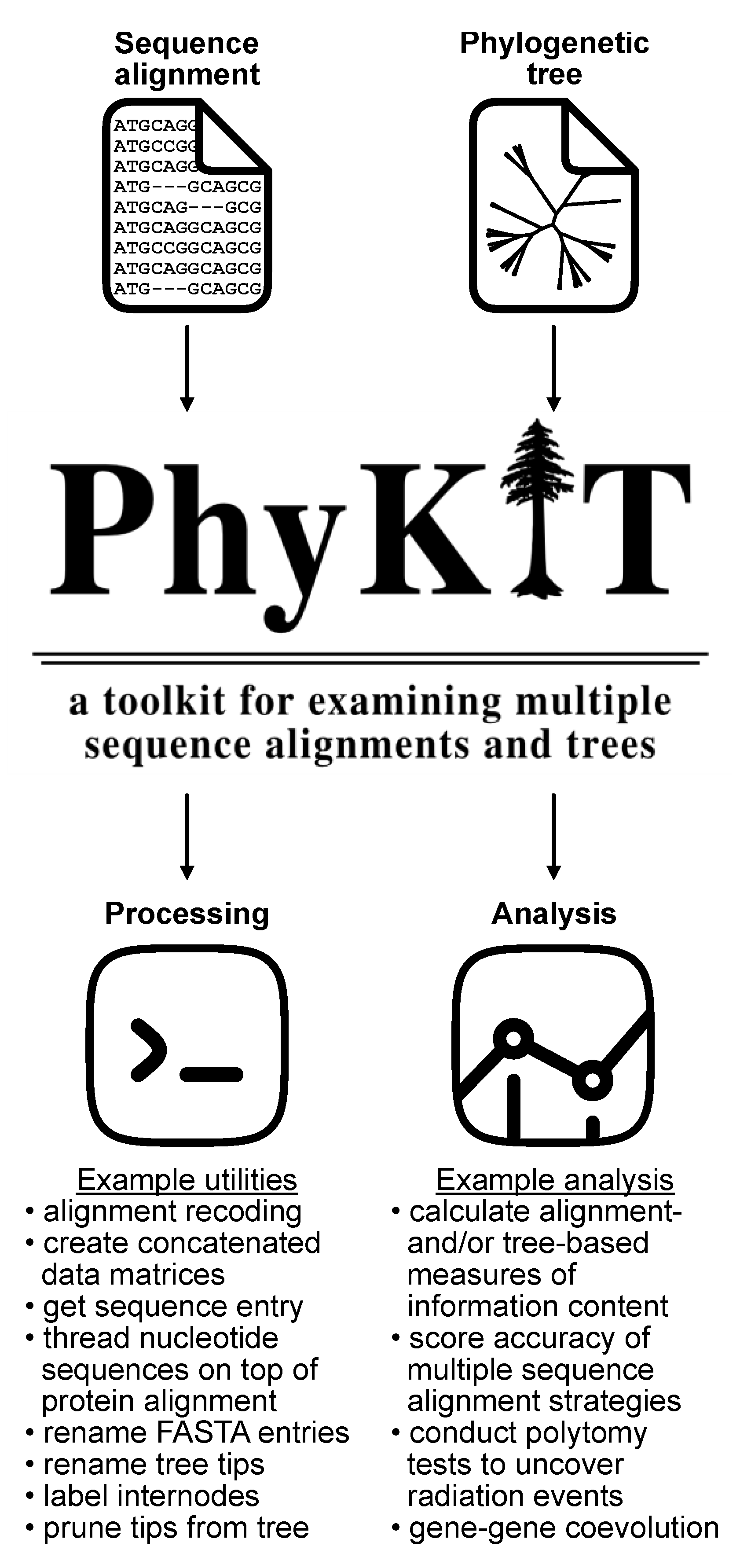
PhyKIT is a software package with multiple functions for high throughput exploration of multiple sequence alignments and phylogenetic trees in phylogenomic datasets (Figure 1 and Table 1) (Steenwyk et al., 2021). This article introduces the basics of processing phylogenomic datasets with PhyKIT, followed by more complex analyses ranging from diagnosing errors and biases in phylogenomic data matrices to identifying radiation events and conducting evolution-based screens to facilitate gene function prediction. Although this article covers frequently used PhyKIT functions, explanations for all 47 utilities are available in the online documentation (https://jlsteenwyk.com/PhyKIT). While these protocols demonstrate how PhyKIT functions democratize the processing and analysis of phylogenomic data matrices, they also underscore how complex phylogenomic analyses can be easily done using a unified toolkit.

Operation System Requirements

Access to a machine with Unix, Linux, Apple OS X, or Windows operating system is required.

Conventions

PhyKIT usage will be depicted as if working in the Unix environment. Unix commands will be in Menlo font, with the $ character indicating the command line. Comments, indicated by the # character, will be used to describe the command being executed and associated output.

Background Knowledge

Previous experience with the Unix command line is assumed. Familiarity with FASTA and Newick file formats—used for multiple sequence alignments and phylogenetic trees, respectively—is also required. FASTA and Newick file formats are the main inputs and outputs of PhyKIT. Files not in these formats can be converted to FASTA or Newick format using software like the sibling toolkit, BioKIT (Steenwyk et al., 2022a), or other utilities like biopython (Cock et al., 2009) and web portals like phylogeny.fr (http://phylogeny.lirmm.fr/phylo_cgi/data_converter.cgi).

Protocol 1: Installing PhyKIT and Syntax for Usage

PhyKIT is freely available under the MIT license via GitHub (https://github.com/JLSteenwyk/PhyKIT) and is distributed through multiple repositories, including Python Package Index (PyPI) (https://pypi.org/project/phykit/) and the Anaconda Cloud (https://anaconda.org/bioconda/phykit). As of writing, the latest PhyKIT release is version 1.19.2. The installed version can easily be updated to the most recent release following the protocol for each distribution platform.

Perhaps the easiest way to install PhyKIT is to use package and environment manager programs like PIP or Conda.

Installing PhyKIT

Install using PIP (Preferred Installer Program)
# install
$ pip install phykit
Install using Conda
# install
$ conda install bioconda::phykit
Install from source
# download
git clone https://github.com/JLSteenwyk/PhyKIT.git
cd PhyKIT/
# install
make install

It may also be useful to install PhyKIT in a separate virtual environment. These isolated environments help separate variable dependencies required by different software, overcoming conflicting dependencies between software (e.g., one software may require an older version of NumPy (Harris et al., 2020)). PhyKIT is engineered to have relatively few dependencies—Biopython, NumPy, SciPy, and Cython (Cock et al., 2009; Harris et al., 2020; Virtanen et al., 2020; Behnel et al., 2011)—to help ensure ease of compatibility with other software and long-term stability. One approach to managing virtual environments is to have one per large project or a substantial portion of a large project. Virtual environments may be stored in the same directory as the project. Ultimately, users must find a system that works best for them. The following are examples of how to install PhyKIT using a virtual environment.

Install in a virtual environment using PIP
# create a virtual environment
$ python -m venv venv_phykit
# activate the virtual environment
$ source venv_phykit/bin/activate
# install
$ pip install PhyKIT

After using software in your virtual environment, you may wish to deactivate (or exit) the virtual environment.

# deactivate virtual environment
deactivate
Install in a virtual environment using Conda
# create a virtual environment
$ conda create -n venv_phykit
# activate the virtual environment
$ conda activate venv_phykit
# install
$ conda install -n venv_phykit bioconda::phykit
# deactivate environment when you are done using PhyKIT
$ conda deactivate

PIP and Conda both have easy ways to automatically check for new software releases and install them if available.

Update installation using PIP
# The “-U” is short for “—upgrade”
$ pip install phykit -U
Update installation using Conda
# This is the same command as to install
$ conda install -n venv_phykit bioconda::phykit
Activate environment before using PhyKIT
If PhyKIT has been installed in an environment, it must be activated when using PhyKIT.
# If installed using PIP activate the environment
$ source venv_phykit/bin/activate
# If installed using Conda, activate the environment
$ conda activate venv_phykit
The PhyKIT help menu
$ phykit -h

If PhyKIT has been successfully installed, this command should return the list of available functions. If installation was unsuccessful, an error message may appear, and users are encouraged to revisit the installation instructions or contact the developers (https://github.com/JLSteenwyk or https://jlsteenwyk.com/contact.html).

PhyKIT functions are organized based on the input file type. Specifically, some functions take multiple sequence alignments as input, others take as input phylogenetic trees, and some functions take both. See Table 1 for a complete list of PhyKIT functions.

PhyKIT functions that take multiple sequence alignment files as input include:

alignment_length: calculates alignment length;
gc_content: calculate GC content of a nucleotide FASTA entries or entries thereof;
pairwise_identity: calculates average pairwise identify among sequences in an alignment file. This is a proxy for evolutionary rate;
relative_composition_variability: calculates relative composition variability in an alignment; and
a complete list of alignment-based functions, including detailed explanations of each, are available here: https://jlsteenwyk.com/PhyKIT/usage/index.html#alignment-based-functions

PhyKIT functions that take phylogenetic trees as input include:

bipartition_support_stats: calculates summary statistics for bipartition support;
degree_of_violation_of_a_molecular_clock: reports the degree of violation of the molecular clock;
evolutionary_rate: reports a tree-based estimation of evolutionary rate for a gene;
prune_tree: prune taxa from a phylogeny; and
a complete list of tree-based functions, including detailed explanations of each, are available here: https://jlsteenwyk.com/PhyKIT/usage/index.html#tree-based-functions

PhyKIT functions that take multiple sequence alignments and phylogenetic trees as input include:

saturation: calculates saturation by examining the slope of patristic distances and uncorrected distances;
treeness_over_rcv: calculates treeness divided by relative composition variability (rcv), treeness, and rcv; and
a complete list of alignment- and tree-based functions, including detailed explanations of each, are available here: https://jlsteenwyk.com/PhyKIT/usage/index.html#alignment-and-tree-based-functions

The help message has abbreviated descriptions of each function. Users are encouraged to read the corresponding section in the documentation (https://jlsteenwyk.com/PhyKIT) for more details about each function. Alternatively, users can print out the help message for specific functions. For example, to see the help message for the alignment_length function, which provides a much more detailed description of the function and its utility, requires executing the following command:

# Call the help message of a specific function
$ phykit alignment_length -h

Throughout the manuscript, we also provide links to relevant documentation of each PhyKIT function, allowing easy access to additional details and explanations of PhyKIT functionality.

PhyKIT Syntax

Although this will be expanded upon in later sections, the syntax of using PhyKIT functions is that users first call PhyKIT, specify the function to be executed, and then specify the arguments required for the function.

# Description of PhyKIT syntax
$ phykit <command> <arguments> [optional arguments]
# Note, optional arguments will always have square brackets around them

For example, the following command demonstrates how to calculate the length of a multiple sequence alignment:

# Calculate alignment length
$ phykit alignment_length input.fa

Function aliases

Every PhyKIT function also has aliases, which are abbreviations of function names. For example, the alignment_length function can also be called using aln_len or al, as exemplified in the following commands:

# Calculate alignment length using the aln_len alias
$ phykit aln_len input.fa
# Calculate alignment length using the al alias
$ phykit al input.fa

Shorthand syntax

To accelerate executing PhyKIT functions, an alternative, shorthand syntax is also available. Specifically, PhyKIT and associated functions can be called by combining the prefix pk_ (shorthand for phykit) with the function name or alias. For example, the shorthand syntax can be used to calculate the length of an alignment using the following command:

# Calculate alignment length using the full function name
$ pk_alignment_length input.fa
# Calculate alignment length using the aln_len alias
$ pk_aln_len input.fa
# Calculate alignment length using the al alias
$ pk_al input.fa

A benefit of the shorthand syntax is the ability to use command-line completion (or tab completion). For example, executing command-line completion after typing pk_ will display all PhyKIT commands and their aliases.

Throughout the remainder of the manuscript, other software that facilitate phylogenomic workflows are mentioned. While aspects of these tools are covered, users are encouraged to read respective installation instructions and documentation.

Summary Statistics and the Verbose Option

Numerous functions report summary statistics. Summary statistics include mean, median, 25th percentile, 75th percentile, minimum, maximum, standard deviation, and variance. For these functions, verbose options (evoked using -v/--verbose) allow every value that generates the underlying values to be reported instead.

Requesting New Functions

Protocols described herein highlight how PhyKIT is a multitool for phylogenomic data processing and analysis. Moreover, PhyKIT is actively undergoing development to serve the research community better, resulting in new functions and additional utilities to existing functions. Thus, users are encouraged to read the PhyKIT documentation for a complete list of functions (https://jlsteenwyk.com/PhyKIT).

If PhyKIT does not have a function that users would want to have, we welcome requests and recommend either contacting the developers via email (https://jlsteenwyk.com/contact.html) or opening a GitHub issue (https://github.com/JLSteenwyk/PhyKIT/issues) with a feature request.

Protocol 2: Constructing a Phylogenomic Supermatrix

Concatenation and the multispecies coalescence are two popular methods for species tree inference (Philippe et al., 2017; Steenwyk et al., 2023a; Gatesy et al., 2017). The concatenation approach requires generating multiple sequence alignments among orthologous loci and combining them into a supermatrix, which is then used to reconstruct evolutionary relationships using a maximum likelihood or Bayesian framework (Philippe et al., 2017; Steenwyk et al., 2023a; Kapli et al., 2020). In contrast, in a popular coalescence-based approach (‘two-step’ coalescence) single-locus phylogenies are first inferred and then the resulting set of trees are used to reconstruct organismal history using, for example, quartet graph construction (Mirarab et al., 2014; Han and Molloy, 2023).

Data Acquisition

Assembled genomes are publicly available from online databases such as GenBank and RefSeq from the National Center for Biotechnology Information (https://www.ncbi.nlm.nih.gov) and the Universal Protein Resource (UniProt) (https://www.uniprot.org). Genomes and transcriptomes can also be de novo assembled using sequencing data available from the Sequence Read Archive (SRA) hosted by the National Center for Biotechnology Information (https://www.ncbi.nlm.nih.gov/sra) or the European Nucleotide Archive (https://www.ebi.ac.uk/ena) hosted by the European Bioinformatics Institute. Data can also be downloaded from dedicated databases such as MolluscDB and MATEdb/2 (Caurcel et al., 2021; Fernández et al., 2022; Martínez-Redondo et al., 2024), among others. Detailed instructions for genome assembly, quality control, and orthology inference are beyond the scope of this manuscript; instead, we cite relevant protocols and briefly describe key steps (Coombe et al., 2023; Manni et al., 2021; Zhao et al., 2023; Raghavan et al., 2022).

Orthology Inference

Next, orthologs are predicted, typically from proteome sequences. De novo orthology can be inferred using, for example, OrthoFinder (Emms and Kelly, 2019). The resulting output can be parsed for single-copy genes. Additional single-copy orthologs nested within larger multi-copy gene families can be identified using OrthoSNAP (Steenwyk et al., 2022b). While methods have been developed to reconstruct evolutionary relationships from gene families with paralogous genes, we focus on phylogenomics using traditional single-copy orthologs and single-copy orthologs identified by OrthoSNAP (Zhang et al., 2020; Steenwyk et al., 2022b). Alternatively, single-copy orthologs can be identified from predetermined single-copy orthologs using tools like BUSCO and orthofisher (Waterhouse et al., 2018; Steenwyk and Rokas, 2021).

Multiple Sequence Alignment and Trimming

Next, single-copy orthologs are aligned and trimmed. During alignment, site-wise homologies are identified across multiple sequences (Steenwyk et al., 2023a; Kapli et al., 2020). Software that infer site-wise homologies include MAFFT, MUSCLE5, or Clustal-Omega (Katoh and Standley, 2013; Edgar, 2022; Sievers and Higgins, 2018) and can be executed using any of the following commands:

# Alignment with MAFFT
$ mafft --auto input.fa > output.fa
# Alignment with MUSCLE5
$ muscle5 -align input.fa -output output.fa
# Alignment with Clustal-Omega
$ clustalo -i input.fa -o output.fa

Subsequently, multiple sequence alignments can be trimmed using ClipKIT or trimAl (Steenwyk et al., 2020; Capella-Gutiérrez et al., 2009). While ClipKIT can be run with default parameters, recent benchmarking studies have demonstrated that all ClipKIT modes perform well (Steenwyk et al., 2020). Here, we demonstrate ClipKIT usage with default parameters. If using trimAl, the same benchmarking studies suggest using the ‘gappyout’ parameter (Tan et al., 2015).

# Trimming with ClipKIT
$ clipkit input.fa -o output.fa
# Trimming with trimAl
$ trimal -in input.fa -out output.fa -gappyout

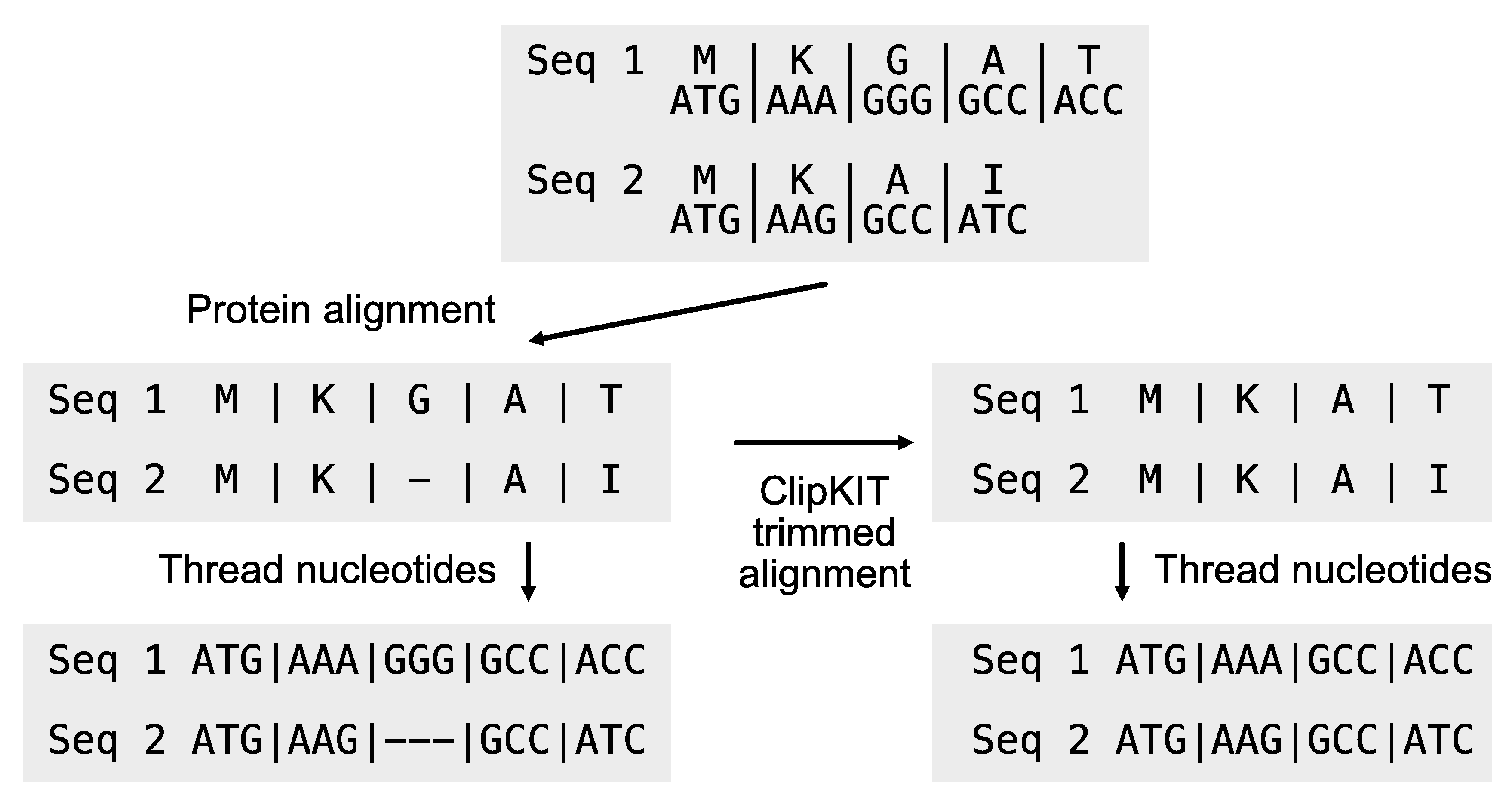
Users may want to create codon-based alignments for phylogenomic inference from DNA sequences. To do so, nucleotide sequences must be threaded on top of protein sequence alignment (Figure 2). The PhyKIT function thread_dna (aliases: pal2nal and p2n; https://jlsteenwyk.com/PhyKIT/usage/index.html#protein-to-nucleotide-alignment) can achieve this. The input files are the multiple sequence alignment protein and the unaligned corresponding nucleotide sequences. To ensure the correct matching between protein and nucleotide sequences, sequences must be identically named in both sequence files. The thread_dna function is executed using the following command:

# Thread nucleotide sequences onto a protein alignment
$ pk_thread_dna -p protein_alignment.faa -n nucleotide_sequences.fna

It is also common to first trim a multiple sequence alignment and then thread the resulting nucleotide sequence onto the trimmed protein alignment. PhyKIT can do so using the log file outputted from ClipKIT. To output the ClipKIT log file, execute the following command, and then use it as an argument to PhyKIT:

# Thread nucleotide sequences onto a trimmed protein alignment
$ clipkit output.fa -o output.fa --log
# Thread nucleotide sequences onto a trimmed protein alignment
$ pk_thread_dna -p protein_alignment.faa -n nucleotide_sequences.fna -l clipkit.log

Alignment recoding—the practice of recoding amino acids and nucleotides to reduced characters sets—can at times combat issues associated with long branch attraction and saturation by multiple substitutions (Giacomelli et al., 2022; Foster et al., 2022; Hernandez and Ryan, 2021). PhyKIT can recode alignments using eight different recoding schemes (Table 2) using the alignment_recoding function (aln_recoding; recode; https://jlsteenwyk.com/PhyKIT/usage/index.html#alignment-recoding). Alternatively, users can recode alignments using custom character schemes.

# Recode alignments
$ pk_aln_recoding input.fa -c <recoding scheme>
# <recoding scheme> can either be one of the eight available
# coding schemes or a file that has the custom coding scheme

Custom recoding schemes should be specified using a two-column file. The first column is the recoded character and the second is the current character in the alignment. For example, the recoding scheme for converting the four nucleotides into a two-character scheme would be as follows:

# Specify custom recoding scheme
$ cat custom_recoding_scheme.txt
A
G
T
C

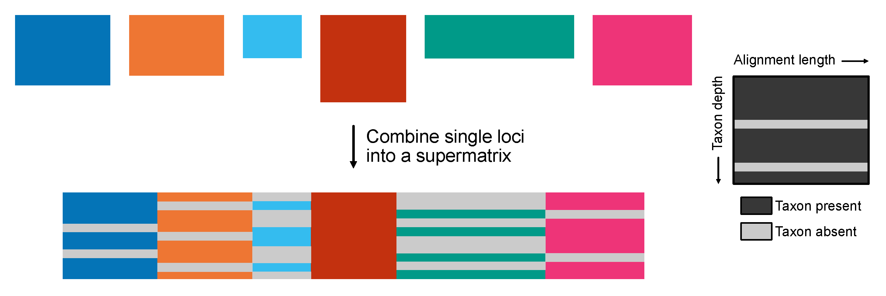
Constructing a Concatenated Supermatrix

The resulting trimmed multiple sequence alignments can be combined into a supermatrix using the PhyKIT function create_concat (Figure 3; https://jlsteenwyk.com/PhyKIT/usage/index.html#create-concatenation-matrix).

# Create concatenation matrix
$ pk_create_concat -a alignment_list.txt -p output_prefix

The create_concat requires two arguments. One argument, -a, is a single-column file with the (absolute or relative) paths to the alignments that will be concatenated. Relative or absolute file paths should be included in the file. An example of how the alignment_list.txt should be formatted is as follows:

# First five lines of the alignment_list.txt file
$ head -n 5 alignment_list.txt
Alignment0.fa
Alignment1.fa
Alignment2.fa
Alignment3.fa
Alignment4.fa

The other argument, -p, will be used as a prefix for the output files. PhyKIT will generate three output files:

output_prefix.fa: the concatenated supermatrix
output_prefix.partition: a description of partition boundaries in RAxML-style format
output_prefix.occupancy: a description of taxon occupancy per partition, including a detailed list of which taxa are present or missing

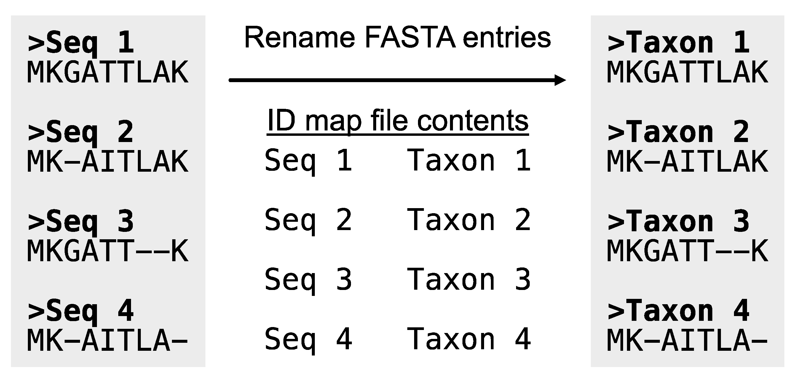
A common error users experience is when one organism is represented by multiple strings across the alignments specified in alignment_list.txt. This may be due to, for example, gene identifiers being included in the FASTA header. PhyKIT requires the same organism to be represented by the same string in the FASTA header. In this way, PhyKIT can determine which sequences belong to the same organism and should, therefore, be concatenated together. If required, the function rename_fasta_entries (alias: rename_fasta) can rename FASTA entry names (Figure 4; https://jlsteenwyk.com/PhyKIT/usage/index.html#rename-fasta-entries). To do so, a two-column file (referred to as an “identifier map” or “ID-map” file must be provided. The ID-map file has two tab-delimited columns: the first column is the current FASTA entry name, and the second column is the new FASTA entry name in the resulting output alignment. For example, the file could be formatted as follows:

# First five lines of the idmap file for renaming FASTA entries
$ head -n 5 idmap.txt
speciesA|gene043 speciesA
speciesB|gene367 speciesB
speciesC|gene589 speciesC
speciesD|gene251 speciesD
speciesE|gene417 speciesE

Subsequently, PhyKIT can be used to rename the FASTA entries using the following command:

# Renaming FASTA entries
$ pk_rename_fasta input.fa -i idmap.txt [-o output.fa]

Once the concatenated gene matrix has been generated, the resulting file can be used as input to software that reconstructs evolutionary histories using maximum likelihood or Bayesian frameworks. The partition file can be used if separate evolutionary models will be used for each locus partition.

Constructing a Dataset for Two-Step Coalescence

Popular coalescence-based software requires a single file populated with single-locus phylogenies as input. To generate this file, the best-fitting substitution model for the multiple sequence alignment as well as the associated single-locus phylogenetic tree must first be inferred. Two popular software for these steps includes ModelTest-NG and ModelFinder within IQ-TREE (Darriba et al., 2020; Minh et al., 2020; Kalyaanamoorthy et al., 2017), which can be executed using either of the following commands:

# ModelTest-NG
$ modeltest-ng -i input.fa -d aa
# IQ-TREE
$ iqtree -s input.fa -m MF

IQ-TREE can also be executed to resemble jModelTest and ProtTest (Darriba et al., 2012, 2011) by changing -m MF to -m TESTONLY.

Subsequently, RAxML-NG or IQ-TREE can infer the single-locus phylogeny using the best-fitting substitution model (Kozlov et al., 2019; Minh et al., 2020) and bipartition support can be examined using 100 bootstrap replicates or 1,000 ultrafast bootstrap approximations, respectively, using the following commands:

# ModelTest-NG
$ raxml-ng --msa prot21.fa --model LG+G4 --prefix output_prefix --bs-trees 100
# IQ-TREE
$ iqtree -s example.phy -m LG+G4 -bb 1000
# Note: LG+G4 should be replaced by the best-fitting substitution model.

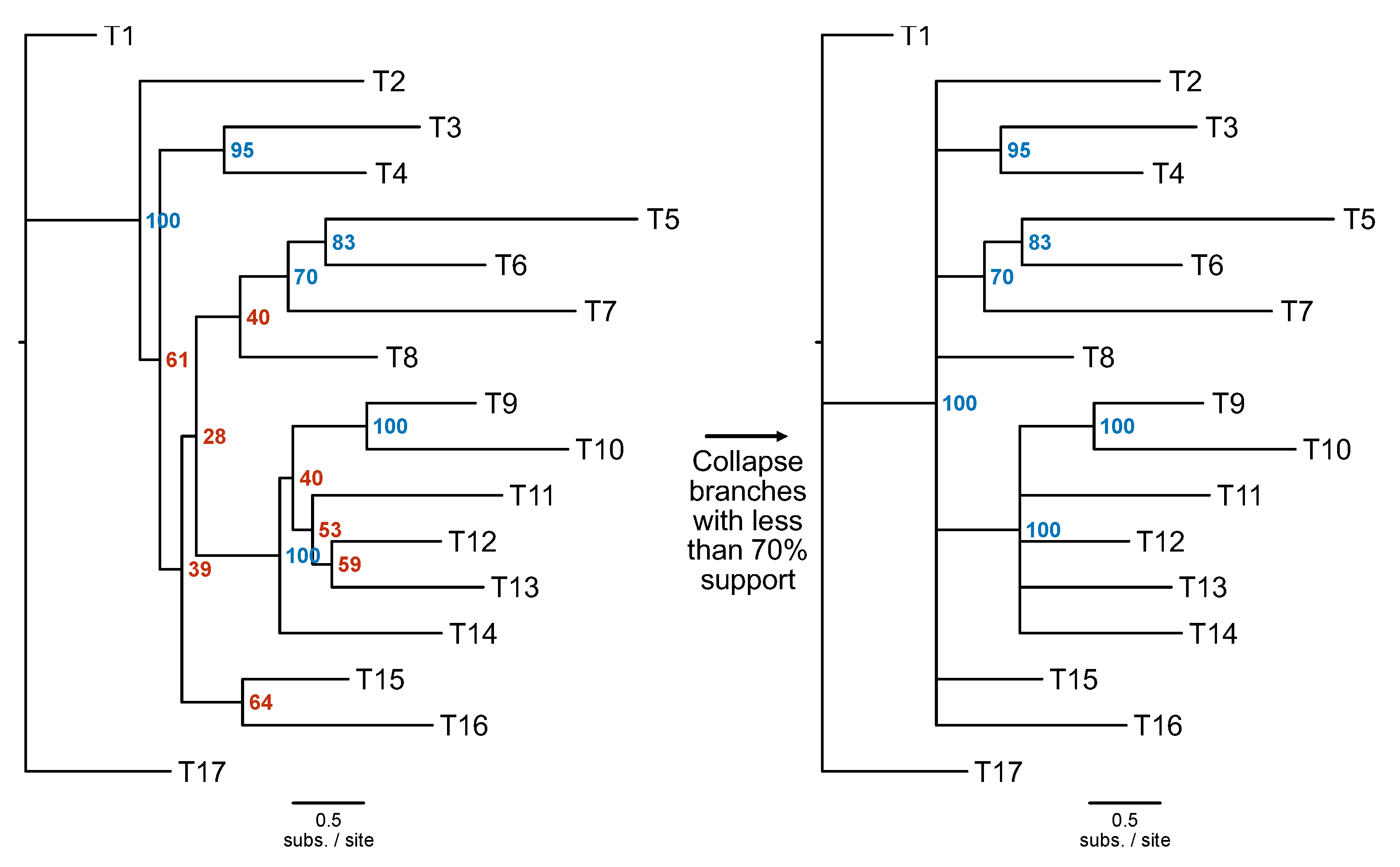
To account for uncertainty in single-locus phylogenies, bipartitions with low support can be collapsed using the PhyKIT function collapse_branches (Figure 5; alias: collapse, cb; https://jlsteenwyk.com/PhyKIT/usage/index.html#collapse-bipartitions). To use this function, users’ must provide the path to the tree file and define a threshold for collapsing bipartitions, which is specified using the -s/--support argument.

# Collapse branches with bipartition support values less than 75
$ pk_collapse input.tre -s 75 [-o output.tre]

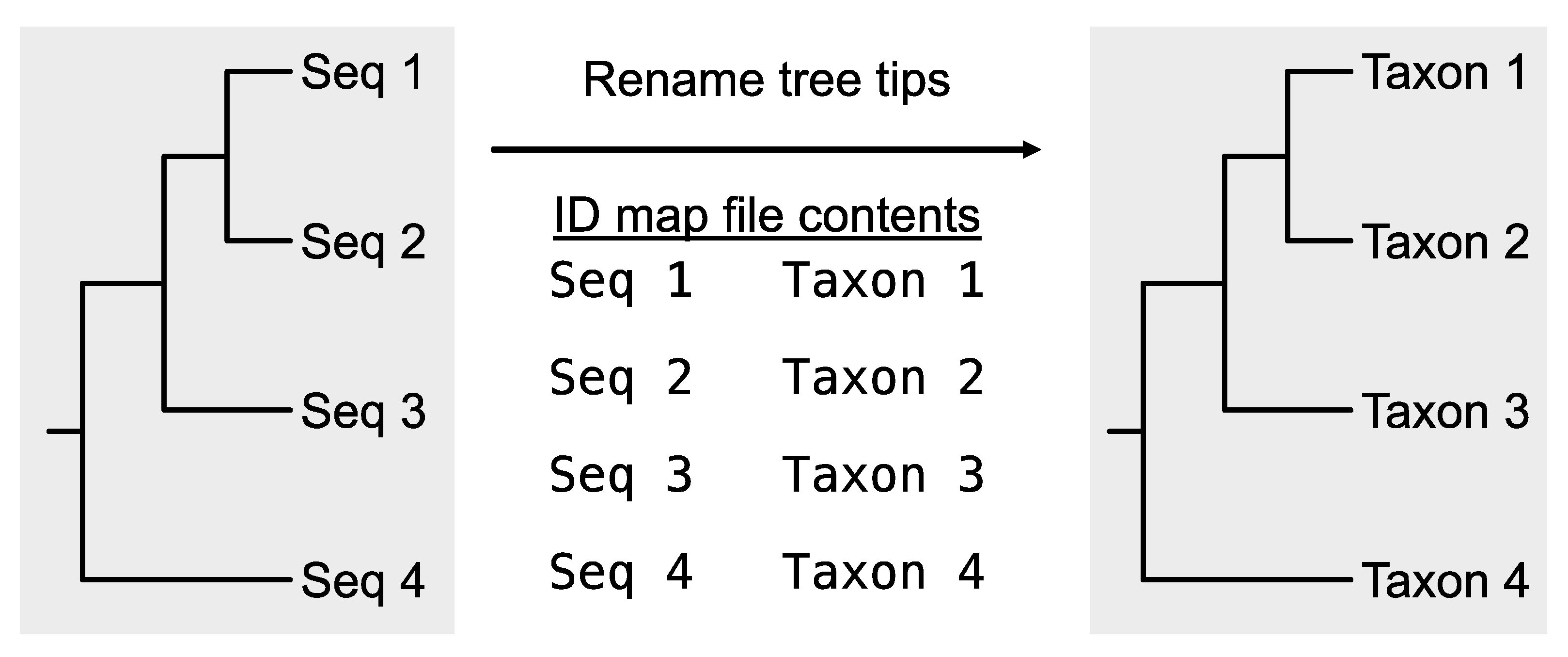
The resulting single-locus phylogenies can be combined into a single file using the cat function. However, software that takes the resulting file as input—such as ASTRAL, Asteroid, or TREE-QMC—typically requires the names of the same organism to be represented by the same string in each tree file. If needed, the PhyKIT function rename_tree_tips (alias: rename_tips) can rename the leaves in a phylogenetic tree using an ID-map file, which is the same two-column file format used in the rename_fasta_entries (Figure 6; https://jlsteenwyk.com/PhyKIT/usage/index.html#rename-tree-tips).

# First five lines of the idmap file for renaming tree tips
$ head -n 5 idmap.txt
speciesA|gene043 speciesA
speciesB|gene367 speciesB
speciesC|gene589 speciesC
speciesD|gene251 speciesD
speciesE|gene417 speciesE

To rename tree tips, use the following command:

# Renaming tips in a phylogenetic tree
$ pk_rename_tree input.tre -i idmap.txt [-o output.tre]

The resulting collection of single-locus phylogenetic trees can be used as input into software that summarizes them using methods that are consistent with the multispecies coalescent model.

Protocol 3: Detecting Anomalies in Orthology Relationships

When constructing phylogenomic data matrices, it is important to consider that errors can be introduced during every step (Steenwyk et al., 2023a). Protocols 3, 4, and 5 help diagnose and sometimes ameliorate diverse sources of error. In this protocol, we will discuss detecting two types of errors in orthology inference – hidden paralogy and spurious ortholog inference.

Hidden Paralogy and Clan Check

Phylogenomics typically relies on single-copy orthologs because they presumably have not undergone a history of duplication and loss (Li et al., 2017; Waterhouse et al., 2018). Hidden paralogs refer to orthologous groups of genes that contain orthologues and paralogues that have undergone asymmetric patterns of duplication and loss (Fernández et al., 2019; Steenwyk et al., 2023a; Martín-Durán et al., 2017). As a result, their evolutionary history can be distinct from the species tree.

Hidden paralogy can be detected by single-loci that do not recover the monophyly of “incontestable” clades, which are defined as lineages broadly accepted to be monophyletic and are often free from phylogenetic controversies (Philippe et al., 2009; Rodríguez-Ezpeleta et al., 2007). For example, it is well accepted that fungi and animals form separate clades (Liu et al., 2023; Ocaña-Pallarès et al., 2022) and single-loci that do not recapitulate the monophyly of each lineage may be subject to complex patterns of duplication and loss. Hidden paralogs also can differ in their phylogenetic information content compared to loci that are not hidden paralogs (Mulhair et al., 2022). Alternatively, hidden paralogy may not be present, but the phylogenetic signal of a single gene may be insufficient to infer such ancient divergences.

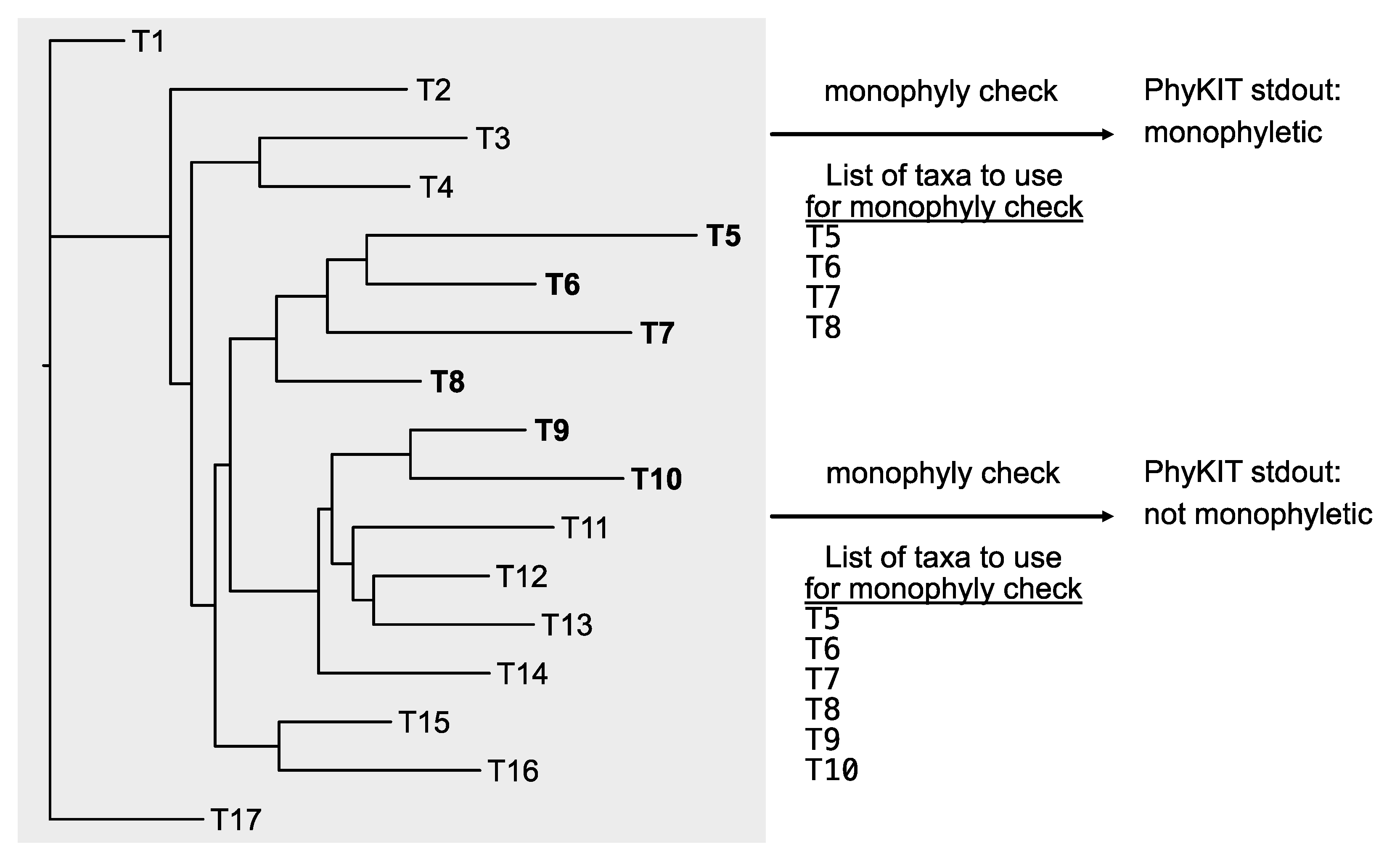
The PhyKIT function monophyly_check (alias: is_monophyletic) can determine if a set of species define a monophyletic group (Figure 7; https://jlsteenwyk.com/PhyKIT/usage/index.html#monophyly-check). The function takes as input two files: a tree file and a single column file with tip names to examine for monophyly. To facilitate high throughput processing, tip names not present in the tree will be excluded when examining monophyly. This function can be executed as follows:

# Monophyly check
$ pk_monophyly_check input.tre list_of_taxa.txt

The output of this function will have six columns: (1) a string reporting if the taxa listed form a monophyletic group; (2) the average, (3) maximum, (4) minimum, and (5) the standard deviation of bipartition support values in the clade of interest; and (6) the names of taxa that are monophyletic with the taxa in list_of_taxa.txt.

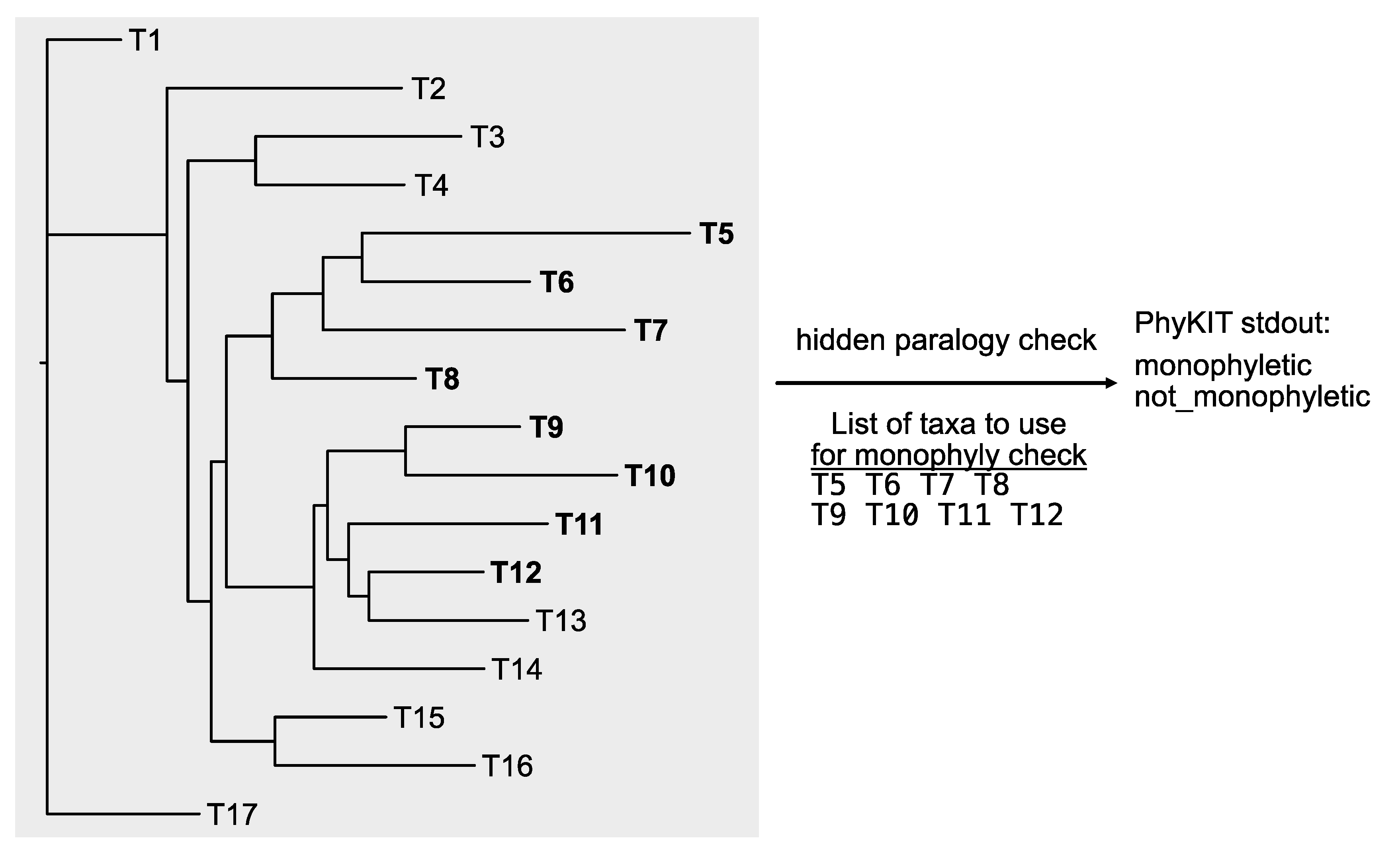
Users may also be interested in examining the exclusive monophyly of multiple sets of taxa, which is an analysis that is often referred to as “clan check” (Mulhair et al., 2022; Siu-Ting et al., 2019). The PhyKIT function hidden_paralogy_check (alias: clan_check) can conduct this analysis (Figure 8; https://jlsteenwyk.com/PhyKIT/usage/index.html#hidden-paralogy-check). To do so, rather than a single column of taxa, each lineage must be provided as a row, and each tip name should be separated by a space (this is termed a “clade file”). For example, suppose it is anticipated that tips T5, T6, T7, and T8 are expected to be monophyletic, and so are T9, T10, T11, and T12. In this case, the clade file should be formatted as follows:

# The format of a clade file
$ cat clades.txt
T6 T7 T8
T10 T11 T12

With an appropriately formatted “clade file,” users can next determine if a single-locus has signatures of hidden paralogy. (However, users should note that other causes, such as lack of signal, may also result in this type of signature.)

# Clan check
$ pk_hidden_paralogy_check input.tre -c clades.txt

The output will report if the specified tips form an exclusively monophyletic group or not. The output will have the same number of rows as specified in the “clade file.” For example, in the exemplary clade file that examines the monophyly of two sets of taxa, there will be two rows of output. The first row corresponds to the result for T5, T6, T7, and T8; the second row corresponds to the result for T9, T10, T11, and T12. In the toy example (Figure 8), PhyKIT will report the first group is exclusively monophyletic and that the second group is not.

Spurious Homolog Detection

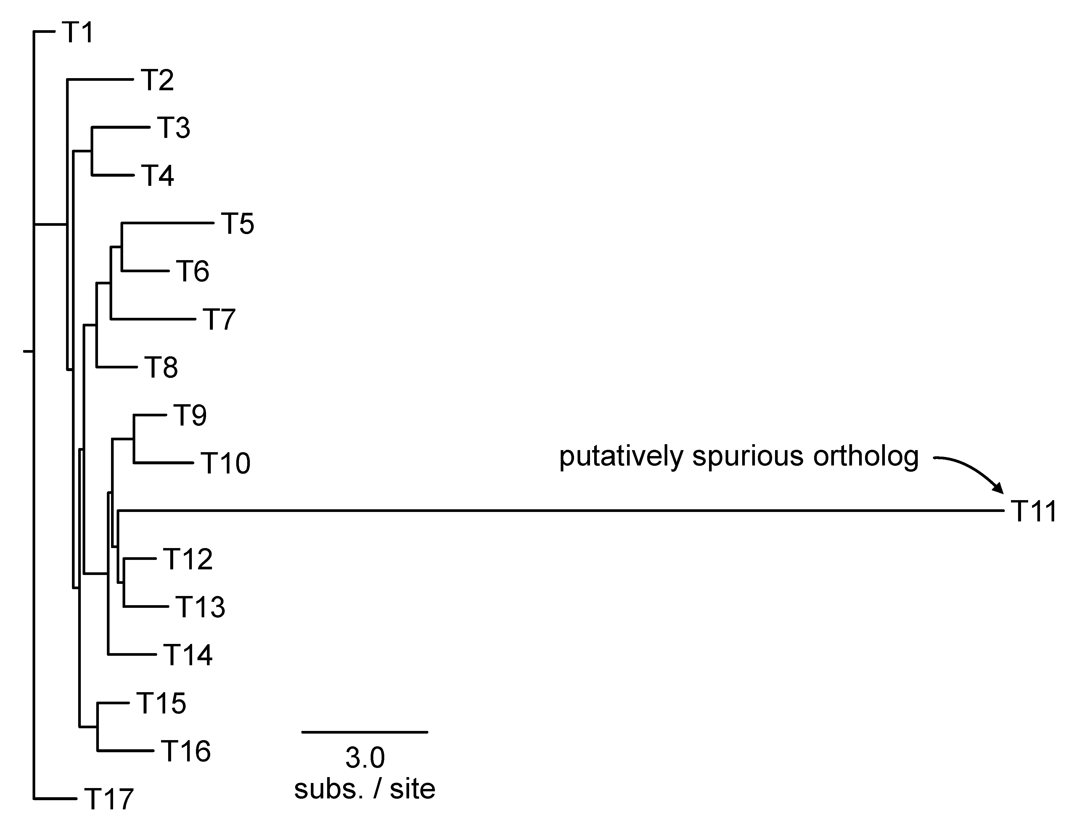
Erroneously inferred sequence homology and orthology can often manifest as long terminal branches (Shen et al., 2018). The PhyKIT function spurious_sequence (aliases: spurious_seq and ss) can be used for detecting long terminal branches (Figure 9; https://jlsteenwyk.com/PhyKIT/usage/index.html#spurious-homolog-identification). Long terminal branches are defined as having X times the median length of all branches in a phylogeny (the default threshold value of X is 20 and can be modified with the -f/--factor argument). This function is executed as follows:

# Identify putatively spurious homologs/orthologs
$ pk_spurious_seq input.tre [-f 20]

The output of this function will have four columns: (1) name of the tip that is a putatively spurious homolog/ortholog; (2) length of branch leading to putatively spurious sequence, (3) threshold used to identify putatively spurious sequences, and (4) median branch length in the phylogeny. The -f argument allows users to modify the threshold value X that defines a “long terminal branch.” Putatively erroneous homologs/orthologs can subsequently be removed from the larger set of sequences before continuing with downstream analyses. To remove sequences from a FASTA file, the BioKIT function remove_fasta_entry can be used (Steenwyk et al., 2022a).

Protocol 4: Quantifying Biases in Phylogenomic Data Matrices and Related Measures

Phylogenomic data matrices may contain biases at the level of the composition of taxa, genes, and sites. PhyKIT employs methods to diagnose potential sources of bias at each of these levels (Table 3). Taxa that may be sources of bias can potentially be removed from phylogenomic data matrices to, for example, examine the stability of a phylogenomic tree inferred using the full dataset (Li et al., 2021; Aberer et al., 2013). At the level of genes, users may want to also select a subset for specific downstream analyses. For example, the stability of a species tree can be examined using phylogenomic subsampling, the practice of subsetting full phylogenomic data matrices for the “best” genes according to a metric and reinferring the species tree (Bjornson et al., 2023; Edwards, 2016; Mongiardino Koch, 2021; Shen et al., 2016; Salichos and Rokas, 2013), or identify genes that evolve in a more clock-like manner for downstream molecular clock analysis (Liu et al., 2017; Smith et al., 2018).

Measuring Bias at the Level of Taxa

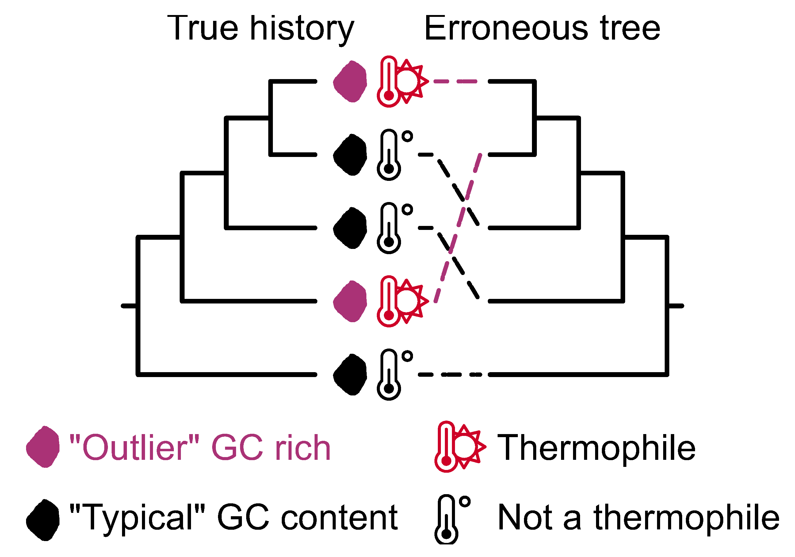
Relative composition variability, taxon (RCVT): Convergent evolution of amino acid or nucleotide usage can challenge phylogenomic inference due to similar sequence changes occurring in independent lineages (Figure 10) (Steenwyk et al., 2023a). For example, high-salt adapted Methanonatronarchaeia and Haloarchaea, two distantly related lineages, have compositional skews of highly acidic amino acids, which can lead to the erroneous inference of phylogenetic affinity (Martijn et al., 2020). Accordingly, users may want to identify taxa with potential compositional biases. The PhyKIT function relative_composition_variability_taxon (alias: rel_comp_var_taxon and rcvt) can quantify biases in individual taxa by calculating RCVT (https://jlsteenwyk.com/PhyKIT/usage/index.html#relative-composition-variability-taxon).

RCVT is derived from a similar metric, relative composition variability (RCV), which was designed to quantify compositional biases in multiple sequence alignments (Phillips and Penny, 2003). RCVT has been adapted to quantify compositional biases in individual taxa rather than across a whole alignment. Specifically, a bias score is calculated for each taxon in an alignment and higher scores indicate higher biases. For example, consider the following toy alignment wherein the first two sequences are skewed toward all Guanines or only Guanines and Cytosines.

# Sequence T1 and T2 are compositionally biased

$ cat toy_alignment.fa

>T1

gggggggggggggggggggg----------------gggggggg

>T2

---------------gggggccccccccccccccccggggggg-

>T3

-----atgcatgcatgcatgcatgcatgcatgc-----------

>T4

-----atgcatgcatgcatgcatgcatgcatgc-----------

>T5

-----atgcatgcatgcatgcatgcatgcatgc-----------

Use the rcvt function to quantify biases in each taxon.

# Quantify relative compositional biases

$ pk_rcvt toy_alignment.fa

T1 0.1436

T2 0.0782

T3 0.0509

T4 0.0509

T5 0.0509

Since T1 and T2 have the highest values, they have the greatest compositional bias in their associated sequences (Table 3). In contrast, T3, T4, and T5 have less bias and lower values. Note that these values should be interpreted relative to one another. Thus, T1 is more compositionally biased than T2 and T3, T4, and T5 have equally low relative compositional bias. To identify taxa that may introduce phylogenomic error, researchers can use outlier detection analysis—such as identifying values outside of the interquartile ranges—across RCVT values to identify taxa with atypical sequences. This analysis can be done via scripting in R or Python.

Long branch score: Long terminal branches can lead to an artifact called long branch attraction wherein distantly related taxa can be inferred as more closely related (Bergsten, 2005; Susko and Roger, 2021). As a result, users may be interested in identifying taxa that can be a source of long branch attraction bias.en The long branch score offers a way to calculate long branch scores for individual taxa and is the mean distance between an individual taxon compared to all other taxa divided by the average distance across every pairwise combination of taxa (Struck, 2014); thus, higher values indicate higher risk for long branch attraction compared to lower values (Table 3). Long branch scores may be calculated in an entire phylogenomic data matrix and the resulting distribution of long branch scores per taxon can be used to identify taxa that may contribute to long branch attraction artifacts.

To provide intuition for the long branch score, consider the following toy phylogeny wherein taxon C has a long terminal branch relative to all other branches (((A:1,B:1):0.5,C:3):0.25,D:1);. To quickly visualize the long branch, print the phylogeny in American Standard Code for Information Interchange (ASCII) format, use the PhyKIT function print_tree (alias: print and pt; https://jlsteenwyk.com/PhyKIT/usage/index.html#print-tree).

# Visualize the toy tree

$ pk_print_tree toy.tre

____________ A

______|

___| |____________ B

| |

_| |____________________________________ C

|____________ D

To calculate long branch scores with PhyKIT, use the long_branch_score function (alias: lb_score and lbs; https://jlsteenwyk.com/PhyKIT/usage/index.html#long-branch-score).

# Quantify long branch scores per taxon

$ pk_lb_score toy.tre -v

A -10.8434

B -10.8434

C 27.7108

D -6.0241

Here, we use an additional argument -v/--verbose, which also reveals that taxon C has the highest long branch score indicating it is on the longest branch; thus, lower values are more desirable. Similarly to RCVT analysis, outlier detection analysis may be useful to identify taxa that may introduce long branch attraction artifacts. Without using the -v/--verbose argument, the summary statistics among the long branch scores per taxon will be reported.

# Quantify summary statistics of long branch score

$ pk_lb_score toy.tre

mean: -0.0

median: -8.4337

25th percentile: -10.8434

75th percentile: 2.4096

minimum: -10.8434

maximum: 27.7108

standard deviation: 18.6131

variance: 346.446

Together, the RCVT and long branch score can help researchers identify taxa that may be sources of phylogenomic error.

Phylogenomic Subsampling Using the Information Content of Alignments

Phylogenomic subsampling can help identify branches in a phylogenomic tree that are unstable (Steenwyk et al., 2023a; Bjornson et al., 2023; Edwards, 2016). Rather than randomly subsampling full data matrices, most studies featuring this approach use metrics associated with phylogenetic signal. Here, we demonstrate how to calculate diverse metrics that collectively summarize the phylogenetic information content in multiple sequence alignments. For sake of brevity, we only briefly introduce each metric, and point users to the relevant documentation for more information. Functions are alphabetically organized to help users quickly find each function. A description of whether high or low values are reflective or greater or lower phylogenetic signal are summarized in Table 3.

Alignment length: Longer alignments are more informative and have been associated with stronger phylogenetic signal (Shen et al., 2016). To calculate the length of an alignment, use the alignment_length (alias: aln_len and al) function in PhyKIT (Figure 11; https://jlsteenwyk.com/PhyKIT/usage/index.html#alignment-length).

# Calculate alignment length

$ pk_aln_len input.fa

Alignment length, no gaps: Gappy sites in alignments may offer little phylogenetic signal and even contribute to noise. The length of an alignment excluding sites with gaps can be calculated with the PhyKIT function alignment_length_no_gaps (Figure 12; alias: aln_len_no_gaps and alng; https://jlsteenwyk.com/PhyKIT/usage/index.html#alignment-length-no-gaps).

# Calculate alignment length excluding sites with gaps

$ pk_alng input.fa

# PhyKIT reports three-tab delimited values.

# col1: number of sites without gaps

# col2: total number of sites

# col3: percentage of sites without gaps

Pairwise identity: Pairwise identity is the average fraction of identical columns for each pairwise combination of sequences in an alignment. As a result, pairwise identity provides an estimate of evolutionary rate (Chen et al., 2017); faster evolving sequences will have lower pairwise identity values, whereas slower evolving sequences will have high pairwise identities. The PhyKIT function pairwise_identity (alias: pairwise_id and pi) can calculate pairwise identities (Figure 13; https://jlsteenwyk.com/PhyKIT/usage/index.html#pairwise-identity).

# Calculate pairwise identity

$ pk_pairwise_id input.fa [-e/--exclude_gaps -v/--verbose]

# Exclude sites with gaps while calculating pairwise identities.

# Obtain identity values for each pair with the verbose option.

Parsimony informative sites: More parsimony informative sites in an alignment is associated with increasing phylogenetic signal (Shen et al., 2016; Steenwyk et al., 2020). The PhyKIT function parsimony_informative_sites (alias: pis) can calculate the number and percentage of parsimony informative sites in an alignment (Figure 14; https://jlsteenwyk.com/PhyKIT/usage/index.html#parsimony-informative-sites).

# Determine the number of parsimony informative sites

$ pk_pis input.fa

# PhyKIT reports three-tab delimited values.

# col1: number of parsimony informative sites

# col2: total number of sites

# col3: percentage of parsimony informative sites

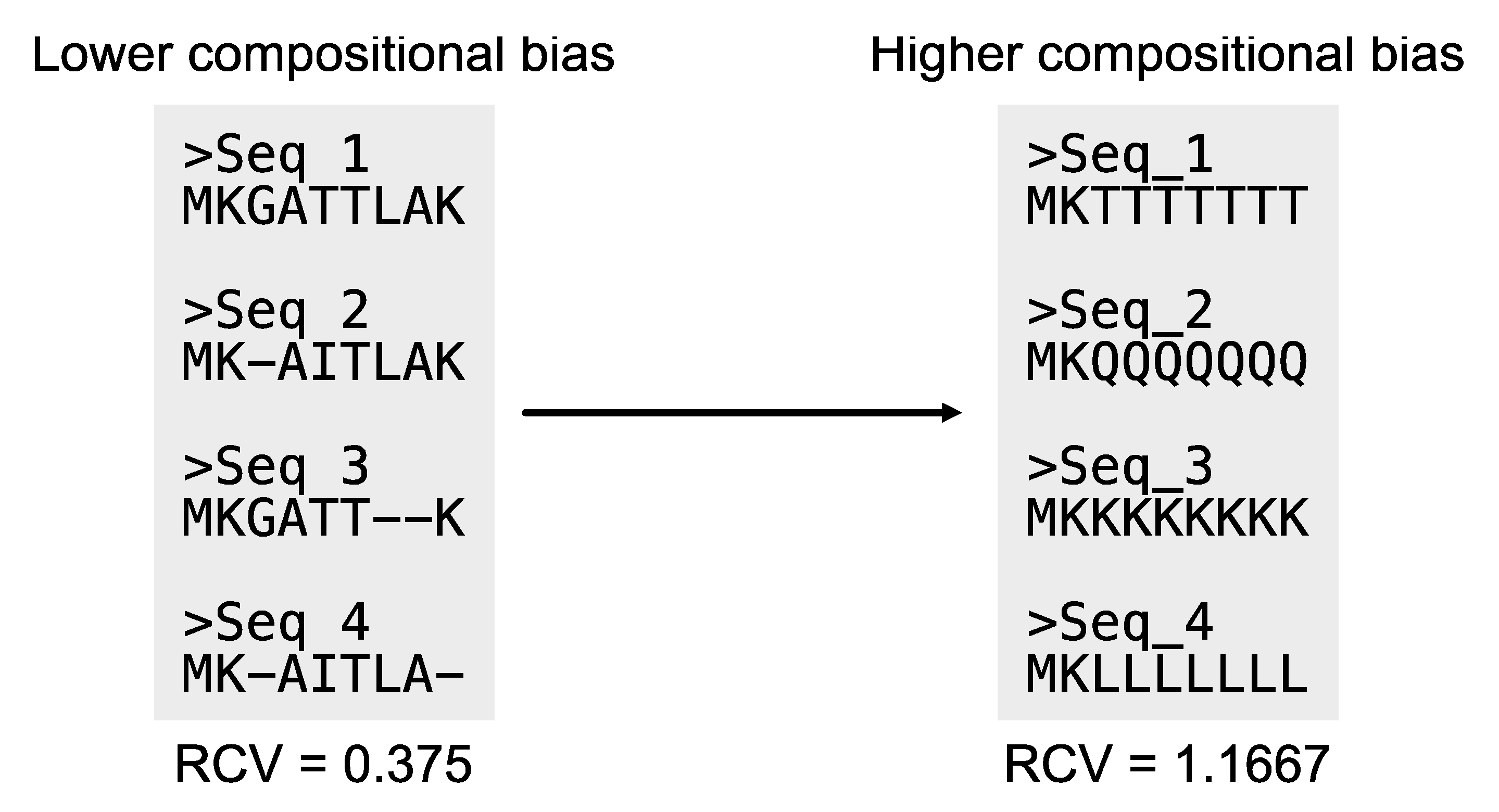
Relative composition variability: As previously noted, compositional biases can introduce phylogenomic errors (Martijn et al., 2020). Relative composition variability (RCV) measures the compositional bias of an alignment (Figure 15). Statistically, RCV describes the average variability in sequence composition among taxa (Phillips and Penny, 2003). Lower RCV values indicate the alignment has lower compositional bias. The PhyKIT function relative_composition_variability (aliases: rel_comp_var and rcv) can calculate RCV for an alignment (https://jlsteenwyk.com/PhyKIT/usage/index.html#relative-composition-variability).

# Determine the number of parsimony informative sites

$ pk_rcv input.fa

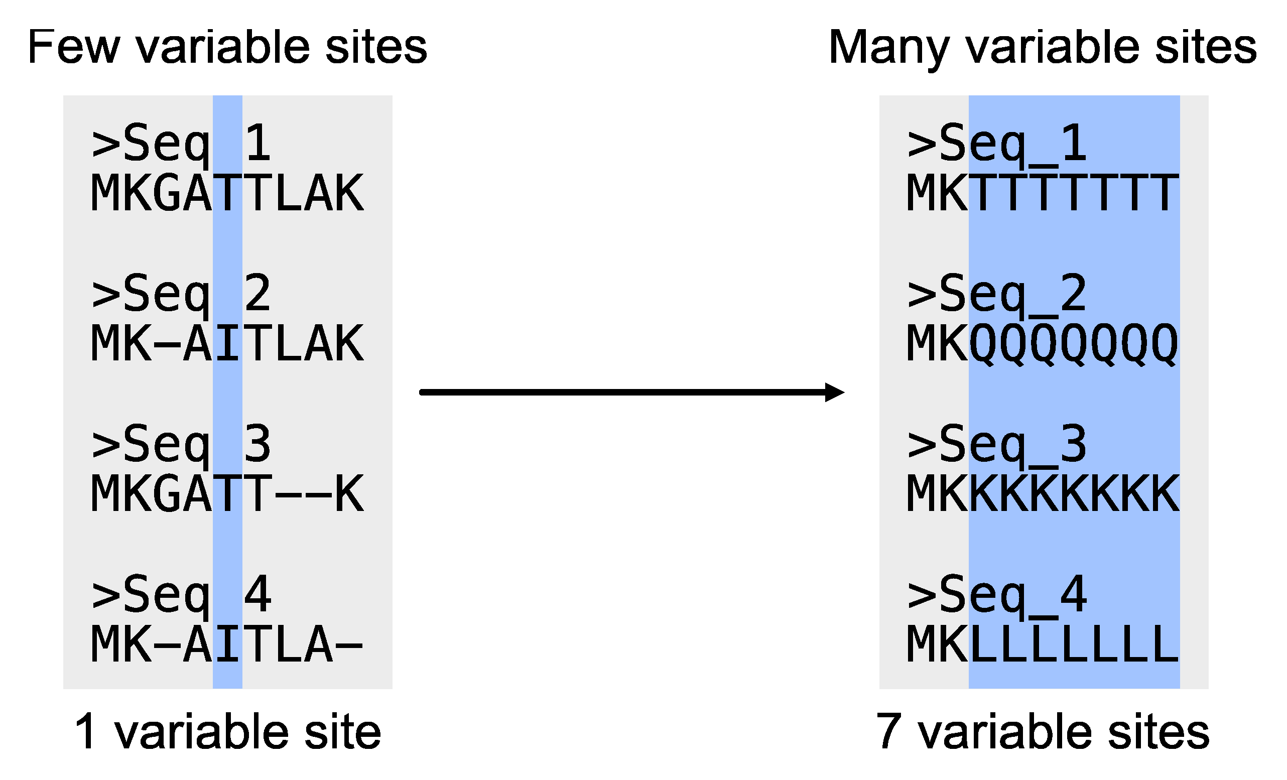
Variable sites: The number of variable sites is associated with phylogenetic signal (Shen et al., 2016). The PhyKIT function variable_sites (alias: vs) can calculate the number and percentage of variable sites in an alignment (Figure 16; https://jlsteenwyk.com/PhyKIT/usage/index.html#variable-sites).

# Determine the number of variable sites

$ pk_vs input.fa

# PhyKIT reports three-tab delimited values.

# col1: number of variable sites

# col2: total number of sites

# col3: percentage of variable sites

Phylogenomic Subsampling Using the Information Content in Phylogenetic Trees

Phylogenomic subsampling may also be conducted based on the features of phylogenetic trees. Here, we demonstrate how to use PhyKIT to calculate diverse metrics that can guide subsampling of full data matrices. Like the previous section, each metric is briefly discussed, and we refer users to the documentation for more information. Functions are alphabetically organized to help users refer back to each function.

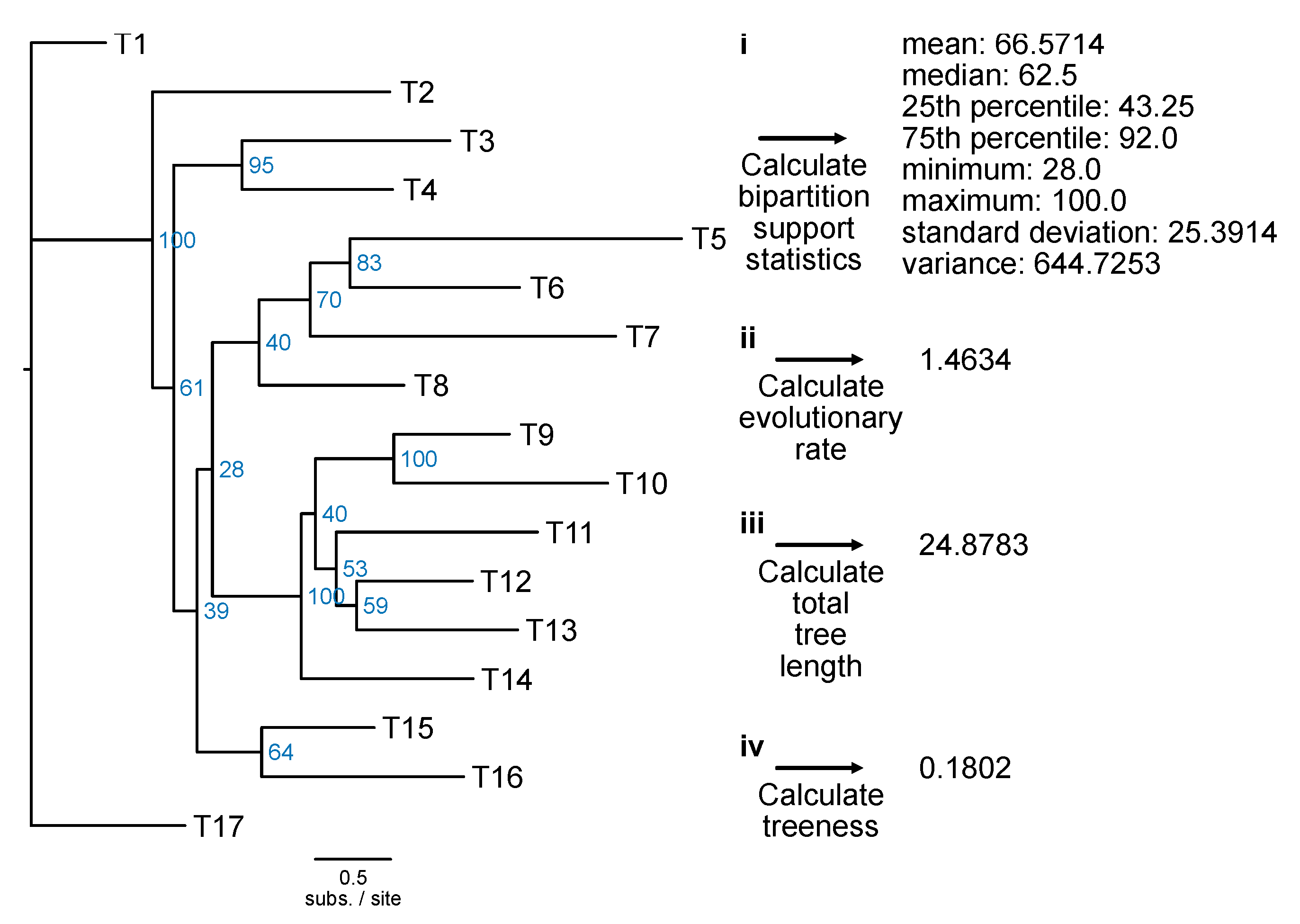
Bipartition support statistics: Single-locus phylogenetic trees that have high overall bootstrap values can help robustly infer ancient divergences (Salichos and Rokas, 2013). The underlying concept is that high support values are indicative of greater certainty in tree topology and, thus, genes with stronger phylogenetic signal. The PhyKIT function bipartition_support_stats (alias: bss) calculates summary statistics of support values in a phylogenetic tree (Figure 17; https://jlsteenwyk.com/PhyKIT/usage/index.html#bipartition-support-statistics).

# Calculate summary statistics of bipartition support

$ pk_bss input.tre

Evolutionary rate: Like pairwise identity, a measure of evolutionary rate using alignment information, the PhyKIT function evolutionary_rate (alias: evo_rate) can calculate evolutionary rate using tree-based information (Figure 17; https://jlsteenwyk.com/PhyKIT/usage/index.html#evolutionary-rate). Specifically, evolutionary rate is the total tree length divided by the number of tips in the tree (Telford et al., 2014).

# Estimate evolutionary rate

$ pk_evo_rate input.tre

Total tree length: Alternatively, total tree length, the sum of all branch lengths, can be used as a proxy for evolutionary rate. The PhyKIT function total_tree_length (alias: tree_len) can be used to calculate the total tree length of a phylogeny (Figure 17; https://jlsteenwyk.com/PhyKIT/usage/index.html#total-tree-length).

# Calculate total tree length

$ pk_tree_len input.tre

Treeness: The signal-to-noise ratio in a phylogenetic tree can be calculated using the metric treeness (Phillips and Penny, 2003). Treeness (which is also referred to as stemminess) is the portion of tree distance among internal branches. Higher treeness values are more desirable because it reflects a higher signal-to-noise ratio. The PhyKIT function treeness (alias: tness) can calculate treeness in a phylogeny (Figure 17; https://jlsteenwyk.com/PhyKIT/usage/index.html#treeness).

# Calculate treeness

$ pk_tness input.tre

Combining the Information Content in Alignments and Trees for Phylogenomic Subsampling

Other measures of phylogenomic subsampling combine information content in multiple sequence alignments and phylogenetic trees.

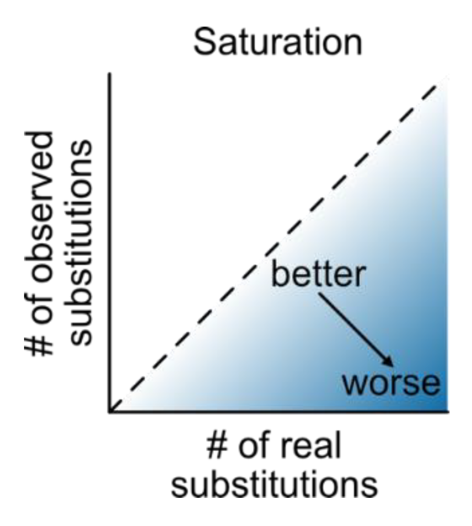
Saturation: Multiple sequence alignments that have undergone numerous substitutions, such that the distances between them are underestimated, saturation is at play (Philippe et al., 2011) (Figure 18). The PhyKIT function saturation (alias: sat) can quantify the level of saturation by multiple substitutions (https://jlsteenwyk.com/PhyKIT/usage/index.html#saturation). Data with no saturation will have a value of 1, while completely saturated data will have a value of 0.

# Calculate saturation

$ pk_tness -a input.fa -t input.tre

Treeness/RCV: Combining the two metrics treeness and RCV—specifically, treeness divided by RCV—allow for identifying loci that harbor a high signal-to-noise ratio and are not very susceptible to compositional bias (Phillips and Penny, 2003). Thus, higher treeness/RCV values are observed among loci with high signal-to-noise ratios and lower compositional biases. The PhyKIT function treeness_over_rcv (alias: toverr and tor) can calculate treeness/RCV.

# Calculate treeness/RCV

$ pk_tor -a input.fa -t input.tre

# PhyKIT reports three-tab delimited values.

# col1: treeness/RCV

# col2: treeness

# col3: RCV

Subsampling for Time Tree Analysis

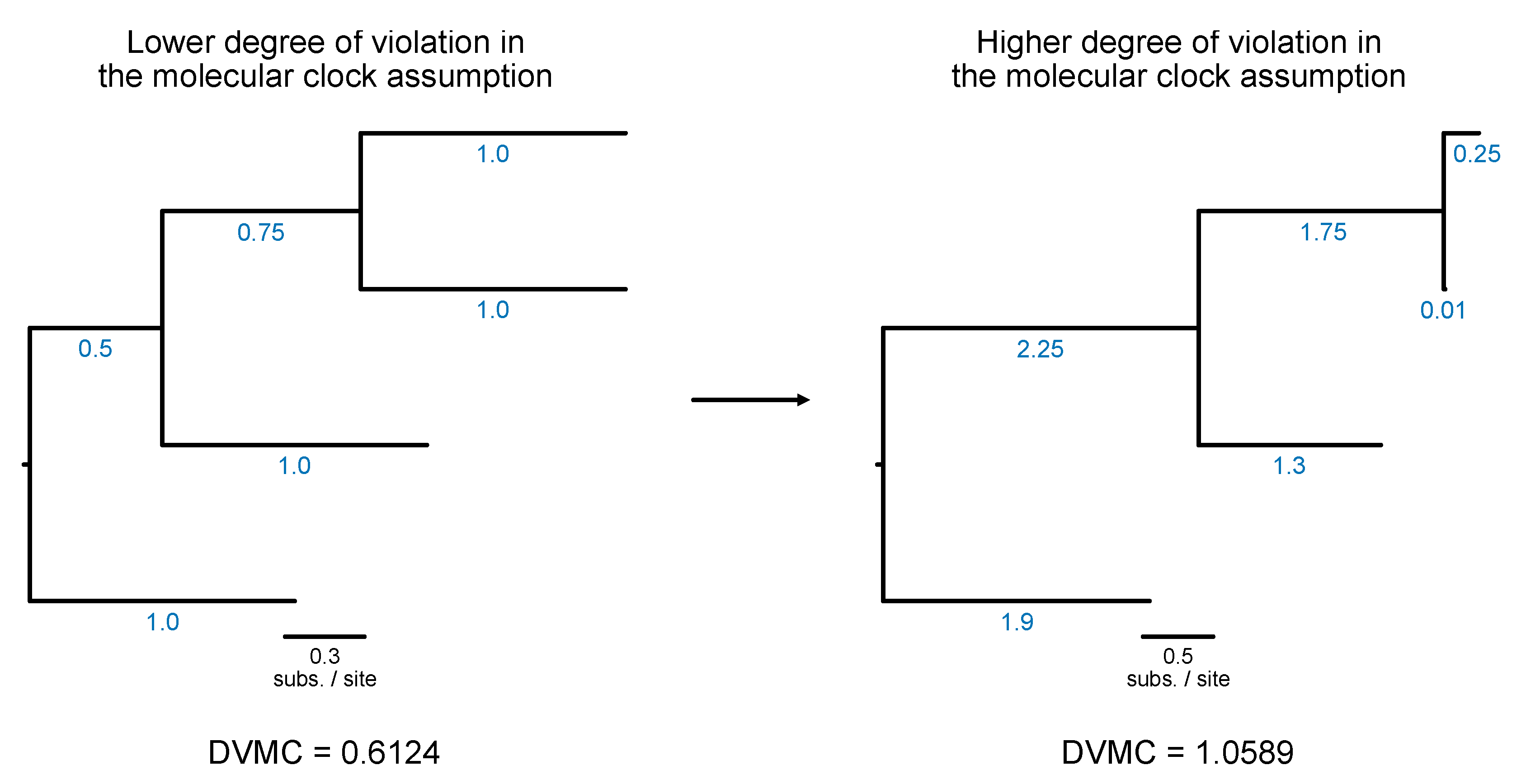
The accuracy of divergence time estimates can be improved by using genes that evolve in a clock-like manner (Smith et al., 2018). The PhyKIT function degree_of_violation_of_a_molecular_clock (alias: dvmc) can quantify how much a gene deviates from a clock-like pattern of evolution (Figure 19; https://jlsteenwyk.com/PhyKIT/usage/index.html#degree-of-violation-of-the-molecular-clock).

# Calculate degree of violation of a molecular clock (or DVMC)

$ pk_dvmc input.tre

Lower values are indicative of a lower degree of violation in the molecular clock assumption; thus, lower values are more desirable for downstream divergence time analysis.

Measuring Bias at the Level of Sites

Compositional bias per site: Compositional biases are known to negatively impact phylogenetic inferences (Phillips and Penny, 2003; Steenwyk et al., 2023a). The PhyKIT function compositional_bias_per_site (alias: comp_bias_per_site and cbps) can quantify compositional biases in an alignment (https://jlsteenwyk.com/PhyKIT/usage/index.html#compositional-bias-per-site). Specifically, site-wise chi-squared tests are conducted to detect compositional biases. Higher chi-squared statistics indicate greater compositional biases. PhyKIT returns multi-test corrected p-values (Benjamini-Hochberg false discovery rate procedure) as well as uncorrected p-values.

# Calculate site-wise compositional biases

$ pk_comp_bias_per_site input.fa

# PhyKIT reports four-tab delimited values.

# col 1: index in alignment

# col 2: chi-squared statistic

# col 3: multi-test corrected p-value

# col 4: uncorrected p-value

Evolutionary rate per site: When saturation is suspected to negatively influence phylogenetic reconstruction, fast-evolving sites are often removed (Eme et al., 2023; Steenwyk et al., 2023a). The PhyKIT function evolutionary_rate_per_site (alias: evo_rate_per_site and erps) quantifies site-wise diversity as a proxy for site-wise evolutionary rate (https://jlsteenwyk.com/PhyKIT/usage/index.html#evolutionary-rate-per-site). Here, the greater the diversity, the greater the presumed evolutionary rate. This is conceptually similar to the use of pairwise identity in an alignment as a measure for evolutionary rate (Chen et al., 2014). Specifically, evolutionary rate per site is one minus the sum of the squared frequency of different characters at a given site. Values range from 0 (slow evolving; no diversity at the given site) to 1 (fast evolving; all characters only appear once).

# Calculate site-wise evolutionary rate

$ pk_evo_rate_per_site input.fa

# PhyKIT reports two-tab delimited values.

# col 1: index in alignment

# col 2: estimated evolutionary rate value

Removing specific sites from an alignment: The resulting output from compositional_bias_per_site and evolutionary_rate_per_site can be used to guide site-specific trimming in a multiple sequence alignment. Site-specific trimming can be conducted using ClipKIT (Steenwyk et al., 2020). For the latter, ClipKIT implements a cst mode of trimming, which is an acronym for “custom-site trimming” (https://jlsteenwyk.com/ClipKIT/advanced/index.html#custom-site-trimming-cst-mode).

# Conduct site-specific trimming

$ clipkit input.fa -m cst -a auxiliary_file.txt

# -m specifies the cst mode

# auxiliary_file.txt specifies which sites to keep/remove

The auxiliary file is a two-column tab-delimited text file wherein the first column is the site (starting at 1) and the second column specifies if the site should be kept or trimmed using the strings “keep” or “trim”.

# Conduct site-specific trimming

$ cat auxiliary_file.txt

1 keep

2 trim

3 keep

4 keep

5 keep

6 keep

Alternatively, users can specify sites that are only kept or trimmed using the auxiliary_file.txt. For example, the following would be equivalent to the auxiliary file described above:

# Conduct site-specific trimming

$ cat auxiliary_file.txt

2 trim

Similarly, users can also only specify sites to keep in the auxiliary_file.txt. The following would be equivalent to the two previous examples:

# Conduct site-specific trimming

$ cat auxiliary_file.txt

1 keep

3 keep

4 keep

5 keep

6 keep

In summary, this protocol demonstrates how to subsample phylogenomic data matrices at the level of taxa, genes and sites. These analyses are aimed to facilitate identifying and ameliorating phylogenomic errors.

Protocol 5: Identifying Polytomies

Polytomies can stem from radiation events or lack of resolution between three alternative topologies in a rooted quartet (Figure 20) (Sayyari and Mirarab, 2018). The signature of a polytomy is when each of the three topologies in a rooted quartet have (near) equal support, which can be tested for using a chi-squared test (Steenwyk et al., 2021). This method has been successfully used to detect polytomies in various fungal and plant lineages (Li et al., 2021; Steenwyk et al., 2021; One Thousand Plant Transcriptomes Initiative, 2019).

To conduct a polytomy test, use the PhyKIT function polytomy_test (alias: polyt and ptt; https://jlsteenwyk.com/PhyKIT/usage/index.html#polytomy-testing). The polytomy_test function takes as input a file with the three groups of taxa to test the relationships.

# format of the groups file is:

# label group0 group1 group2

$ cat groups.txt

name_of_test T1;T2 T3 T4;T5

A single column file with the names of the desired tree files to use for polytomy testing must also be specified.

# label group0 group1 group2

$ cat trees.txt

Input0.tre

Input1.tre

Input2.tre

Input3.tre

…

Using the two files, conduct a polytomy test.

# Conduct a polytomy test

$ pk_ptt -t trees.txt -g groups.txt

To test conducting a polytomy test using real data, see the online documentation (https://jlsteenwyk.com/PhyKIT/tutorials/index.html#identifying-signatures-of-rapid-radiations).

Protocol 6: Gene-Gene Coevolution as a Genetic Screen

Genes that coevolve tend to have shared function, be coexpressed, or be constituents of the same multimeric complex (Clark et al., 2012; Steenwyk et al., 2022c). Moreover, gene coevolution can be used to prioritize genes with a predicted functionality via guilt-by-association. For example, genes that are coevolving with other genes that function in DNA repair processes can be rapidly screened to identify additional DNA repair genes (Brunette et al., 2019).

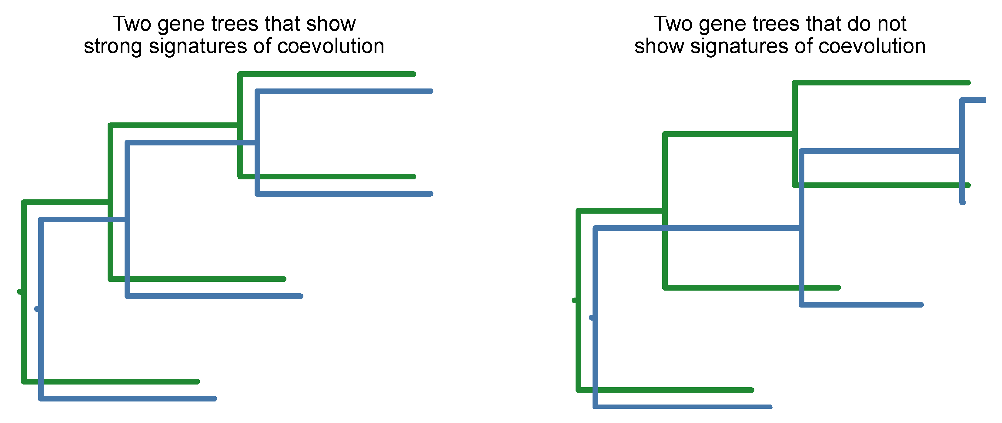
Gene coevolution can be detected by the mirror principle wherein two gene trees have similar branch lengths across speciation events (Steenwyk et al., 2022c). In other words, two phylogenetic trees accelerate and decelerate in evolutionary rates in a coordinated manner (Figure 21). To avoid false positives, gene tree branch lengths need to be corrected by the corresponding branch length in a species tree (Clark et al., 2012; Steenwyk et al., 2022c). Moreover, this corrects to variation in branch lengths associated with differences in mutation and divergence time.

To quantify gene coevolution, the cover function in PhyKIT is used (https://jlsteenwyk.com/PhyKIT/usage/index.html#covarying-evolutionary-rates). The cover function takes as input two single-locus phylogenies and a reference species tree

# Executing the cover function

$ pk_cover tree1.tre tree2.tre -r reference_tree.tre

# PhyKIT outputs two values

# col 1: coevolutionary coefficient (the strength of coevolution)

# col 2: p-value

PhyKIT requires that the three phylogenies have the same topology; that is, the two single-locus phylogenies should be constrained to match the reference tree. To perform constrained tree search using IQ-TREE (Minh et al., 2020), the following command can be used:

# constrained tree search

$ iqtree2 -s tree1.fa -te reference_tree.constrained_topology.tre -pre output_prefix -m TEST -keep-ident

The resulting phylogeny should be rooted following the reference tree using the root_tree (alias: root and rt) function or other software. PhyKIT automatically accounts for variation in taxon representation between two single-locus phylogenies. Thereafter, gene coevolution can be quantified. A tutorial of gene-gene coevolution using real data is available in the online documentation (https://jlsteenwyk.com/PhyKIT/tutorials/index.html#evaluating-gene-gene-covariation).

Commentary

Related Tools

PhyKIT was initially developed to overcome the absence of transversal phyloinformatic tools available for some key steps in data processing and analysis of phylogenomic data. Specifically, PhyKIT was developed to quantify biases in phylogenomic data matrices and calculate gene-gene coevolution. However, while developing PhyKIT, we recognized the opportunity to provide broader support to the phyloinformatic community. We were excited to provide a broadly applicable tool and were excited (and surprised!) to see it be adopted by the community.

Since initially releasing PhyKIT, we have developed several other tools that may be of interest to readers. Together, these tools are part of a broader ecosystem of bioinformatic tools that facilitate phylogenomic data analysis, processing, and more.

ClipKIT, an alignment trimming software (Steenwyk et al., 2020);

○

Documentation: https://jlsteenwyk.com/ClipKIT/

○

Source code: https://github.com/JLSteenwyk/ClipKIT
BioKIT, a broadly applicable toolkit for broad genomic analysis (Steenwyk et al., 2022a);

○

Documentation: https://jlsteenwyk.com/BioKIT/

○

Source code: https://github.com/JLSteenwyk/BioKIT
OrthoSNAP, an algorithm to identify single-copy orthologs nested within larger multi-copy gene families (Steenwyk et al., 2022b);

○

Documentation: https://jlsteenwyk.com/orthosnap/

○

Source code: https://github.com/JLSteenwyk/orthosnap
orthofisher, software for sequence similarity search using Hidden Markov Models (Steenwyk and Rokas, 2021);

○

Documentation: https://jlsteenwyk.com/orthofisher/

○

Source code: https://github.com/JLSteenwyk/orthofisher
treehouse, a graphical user interface tool for pruning large phylogenies (Steenwyk and Rokas, 2019);

○

Documentation and source code: https://github.com/JLSteenwyk/treehouse
ggpubfigs, a ggplot2 extension (https://ggplot2.tidyverse.org/) for making colorblind-friendly and publication-quality scientific figures

○

Documentation and source code: https://github.com/JLSteenwyk/ggpubfigs

These, alongside other software, have been incorporated into a Snakemake workflow, Orthoflow (https://github.com/rbturnbull/orthoflow), to enable phylogenomic analysis using one command (Turnbull et al., 2023).

Troubleshooting

Users can submit GitHub issues for support (https://github.com/JLSteenwyk/PhyKIT/issues) or contact the lead developer via email (https://jlsteenwyk.com/contact.html).

Future Directions

Further development of PhyKIT will be guided by the best practices and advances in the field. Currently, alternative data types (e.g., synteny or structure information) are becoming more common in phylogenomics (Parey et al., 2023; Schultz et al., 2023; Steenwyk and King, 2023). The utility of PhyKIT for alternative data types will be explored. We anticipate that certain metrics will be easily transferred to other data types (e.g., bipartition support statistics or treeness) because they handle phylogenetic trees, not the underlying data used to infer them.

Acknowledgements

PhyKIT has benefitted from the kindness and generosity of the research community. A special thanks to Drs. Michael F. Seidl, Jason Stajich, Toby Baril, and Heroen Verbruggen for helpful comments and suggestions. JLS is a Howard Hughes Medical Institute Awardee of the Life Sciences Research Foundation. Research in AR’s lab is supported by grants from the National Science Foundation (DEB-2110404), the National Institutes of Health/National Institute of Allergy and Infectious Diseases (R01 AI153356), and the Burroughs Wellcome Fund. GIMR acknowledges the support of Secretaria d’Universitats i Recerca del Departament d’Empresa i Coneixement de la Generalitat de Catalunya and ESF Investing in your future (grant 2021 FI_B 00476). X-XS was supported by the National Key R&D Program of China (2022YFD1401600) and the National Science Foundation for Distinguished Young Scholars of Zhejiang Province (LR23C140001). RF acknowledges support from the following sources of funding: Ramón y Cajal fellowship (grant agreement no. RYC2017-22492 funded by MCIN/AEI /10.13039/501100011033 and ESF ‘Investing in your future’), the European Research Council (this project has received funding from the European Research Council (ERC) under the European’s Union’s Horizon 2020 research and innovation programme (grant agreement no. 948281)) and the Secretaria d’Universitats i Recerca del Departament d’Economia i Coneixement de la Generalitat de Catalunya (AGAUR 2021-SGR00420).

Conflicts of interest: JLS is an advisor for ForensisGroup Inc. AR is a scientific consultant for LifeMine Therapeutics, Inc.

Glossary

Bootstrap replicates	In the context of phylogenetics, each replicate is a resampling (with replacement) of sites from the full alignment to generate an alignment of equal size; these replicates are then used to reinfer a phylogeny and evaluate support for the phylogeny inferred using the full alignment.
Concatenation	The phylogenomic method of combining sequences from multiple loci into a single sequence for each species and using the resulting supermatrix for species tree inference.
Hidden paralogy	Asymmetric loss of paralogs in some lineages, leading to mistaken identification of paralogs as orthologs.
Long branch attraction	A phylogenetic artifact where rapidly evolving taxa/lineages are erroneously inferred to be closely related.
Multispecies coalescence	The phylogenomic method of using single-locus phylogenies, which may differ from each other, to infer a species tree.
Orthologs or orthologous genes	Genes in different species that originated from a common ancestor by speciation.
Orthology inference	Identifying genes among organisms that evolved from a common ancestral gene.
Paralogs or paralogous genes	Genes that are related by duplication.
Phylogenomic subsampling	The process of selecting a subset of a complete phylogenomic data matrix to reconstruct phylogenetic trees, often aiming to reduce noise and improve signal or evaluating the stability of the inferred phylogeny.
Radiation events	Rapid speciation events that result in a succession of short internal branches in a phylogeny.
Single-copy orthologs	Genes present as a single copy in the genome across a set of taxa and originate from speciation events.
Spurious ortholog inference	Incorrect identification of genes as orthologous, often due to errors in sequence analysis or interpretation.

References

Aberer, A. J.; Krompass, D.; Stamatakis, A. Pruning Rogue Taxa Improves Phylogenetic Accuracy: An Efficient Algorithm and Webservice. Systematic Biology, 2013; 62, 162–166. [Google Scholar]
Behnel, S., Bradshaw, R., Citro, C., Dalcin, L., Seljebotn, D. S., and Smith, K. 2011. Cython: The Best of Both Worlds. Computing in Science & Engineering 13:31–39.
Bergsten, J. A review of long-branch attraction. Cladistics, 2005; 21, 163–193. [Google Scholar]
Bjornson, S., Upham, N., Verbruggen, H., and Steenwyk, J. 2023. Phylogenomic Inference, Divergence-Time Calibration, and Methods for Characterizing Reticulate Evolution. Biology and Life Sciences Available at: https://www.preprints.org/manuscript/202309.0905/v1 [Accessed September 25, 2023].
Brunette, G. J., Jamalruddin, M. A., Baldock, R. A., Clark, N. L., and Bernstein, K. A. 2019. Evolution-based screening enables genome-wide prioritization and discovery of DNA repair genes. Proceedings of the National Academy of Sciences 116:19593–19599.
Capella-Gutiérrez, S., Silla-Martínez, J. M., and Gabaldón, T. 2009. trimAl: a tool for automated alignment trimming in large-scale phylogenetic analyses. Bioinformatics 25:1972–1973.
Caurcel, C., Laetsch, D. R., Challis, R., Kumar, S., Gharbi, K., and Blaxter, M. 2021. MolluscDB: a genome and transcriptome database for molluscs. Philosophical Transactions of the Royal Society B: Biological Sciences 376:20200157.
Chen, M.-Y., Liang, D., and Zhang, P. 2017. Phylogenomic Resolution of the Phylogeny of Laurasiatherian Mammals: Exploring Phylogenetic Signals within Coding and Noncoding Sequences. Genome Biology and Evolution 9:1998–2012.
Chen, W., Lee, M.-K., Jefcoate, C., Kim, S.-C., Chen, F., and Yu, J.-H. 2014. Fungal Cytochrome P450 Monooxygenases: Their Distribution, Structure, Functions, Family Expansion, and Evolutionary Origin. Genome Biology and Evolution 6:1620–1634.
Clark, N. L., Alani, E., and Aquadro, C. F. 2012. Evolutionary rate covariation reveals shared functionality and coexpression of genes. Genome Research 22:714–720.
Cock, P. J. A., Antao, T., Chang, J. T., Chapman, B. A., Cox, C. J., Dalke, A., Friedberg, I., Hamelryck, T., Kauff, F., Wilczynski, B., et al. 2009. Biopython: freely available Python tools for computational molecular biology and bioinformatics. Bioinformatics 25:1422–1423.
Coombe, L., Warren, R. L., Wong, J., Nikolic, V., and Birol, I. 2023. ntLink: A Toolkit for De Novo Genome Assembly Scaffolding and Mapping Using Long Reads. Current Protocols 3:e733.
Darriba, D., Posada, D., Kozlov, A. M., Stamatakis, A., Morel, B., and Flouri, T. 2020. ModelTest-NG: A New and Scalable Tool for the Selection of DNA and Protein Evolutionary Models. Molecular Biology and Evolution 37:291–294.
Darriba, D., Taboada, G. L., Doallo, R., and Posada, D. 2012. jModelTest 2: more models, new heuristics and parallel computing. Nature Methods 9:772–772.
Darriba, D., Taboada, G. L., Doallo, R., and Posada, D. 2011. ProtTest 3: fast selection of best-fit models of protein evolution. Bioinformatics 27:1164–1165.
Delsuc, F., Brinkmann, H., and Philippe, H. 2005. Phylogenomics and the reconstruction of the tree of life. Nature Reviews Genetics 6:361–375.
Edgar, R. C. 2022. Muscle5: High-accuracy alignment ensembles enable unbiased assessments of sequence homology and phylogeny. Nature Communications 13:6968.
Edwards, S. V. 2016. Phylogenomic subsampling: a brief review. Zoologica Scripta 45:63–74.
Eisen, J. A. 1998. Phylogenomics: Improving Functional Predictions for Uncharacterized Genes by Evolutionary Analysis. Genome Research 8:163–167.
Embley, M., Der Giezen, M. V., Horner, D. S., Dyal, P. L., and Foster, P. 2003. Mitochondria and hydrogenosomes are two forms of the same fundamental organelle. Philosophical Transactions of the Royal Society of London. Series B: Biological Sciences 358:191–203.
Eme, L., Tamarit, D., Caceres, E. F., Stairs, C. W., De Anda, V., Schön, M. E., Seitz, K. W., Dombrowski, N., Lewis, W. H., Homa, F., et al. 2023. Inference and reconstruction of the heimdallarchaeial ancestry of eukaryotes. Nature 618:992–999.
Emms, D. M., and Kelly, S. 2019. OrthoFinder: phylogenetic orthology inference for comparative genomics. Genome Biology 20:238.
Fernández, R., Gabaldón, T., and Dessimoz, C. 2019. Orthology: definitions, inference, and impact on species phylogeny inference. Available at: https://arxiv.org/abs/1903.04530 [Accessed May 25, 2023].
Fernández, R., Tonzo, V., Simón Guerrero, C., Lozano-Fernandez, J., Martínez-Redondo, G. I., Balart-García, P., Aristide, L., Eleftheriadi, K., and Vargas-Chávez, C. 2022. MATEdb, a data repository of high-quality metazoan transcriptome assemblies to accelerate phylogenomic studies. Peer Community Journal 2:e58.
Foster, P. G., Schrempf, D., Szöllősi, G. J., Williams, T. A., Cox, C. J., and Embley, T. M. 2022. Recoding Amino Acids to a Reduced Alphabet may Increase or Decrease Phylogenetic Accuracy. Systematic Biology:syac042.
Gatesy, J., Meredith, R. W., Janecka, J. E., Simmons, M. P., Murphy, W. J., and Springer, M. S. 2017. Resolution of a concatenation/coalescence kerfuffle: partitioned coalescence support and a robust family-level tree for Mammalia. Cladistics 33:295–332.
Giacomelli, M., Rossi, M. E., Lozano-Fernandez, J., Feuda, R., and Pisani, D. 2022. Resolving tricky nodes in the tree of life through amino acid recoding. iScience 25:105594.
Green, R. E., Braun, E. L., Armstrong, J., Earl, D., Nguyen, N., Hickey, G., Vandewege, M. W., St. John, J. A., Capella-Gutiérrez, S., Castoe, T. A., et al. 2014. Three crocodilian genomes reveal ancestral patterns of evolution among archosaurs. Science 346:1254449.
Han, Y., and Molloy, E. K. 2023. Improving quartet graph construction for scalable and accurate species tree estimation from gene trees. Genome Research:genome;gr.277629.122v2.
Harris, C. R., Millman, K. J., Van Der Walt, S. J., Gommers, R., Virtanen, P., Cournapeau, D., Wieser, E., Taylor, J., Berg, S., Smith, N. J., et al. 2020. Array programming with NumPy. Nature 585:357–362.
Hernandez, A. M., and Ryan, J. F. 2021. Six-State Amino Acid Recoding is not an Effective Strategy to Offset Compositional Heterogeneity and Saturation in Phylogenetic Analyses. Systematic Biology 70:1200–1212.
Jarvis, E. D., Mirarab, S., Aberer, A. J., Li, B., Houde, P., Li, C., Ho, S. Y. W., Faircloth, B. C., Nabholz, B., Howard, J. T., et al. 2014. Whole-genome analyses resolve early branches in the tree of life of modern birds. Science 346:1320–1331.
Kalyaanamoorthy, S., Minh, B. Q., Wong, T. K. F., Von Haeseler, A., and Jermiin, L. S. 2017. ModelFinder: fast model selection for accurate phylogenetic estimates. Nature Methods 14:587–589.
Kapli, P., Yang, Z., and Telford, M. J. 2020. Phylogenetic tree building in the genomic age. Nature Reviews Genetics 21:428–444.
Katoh, K., and Standley, D. M. 2013. MAFFT Multiple Sequence Alignment Software Version 7: Improvements in Performance and Usability. Molecular Biology and Evolution 30:772–780.
Kosiol, C., Goldman, N., and H. Buttimore, N. 2004. A new criterion and method for amino acid classification. Journal of Theoretical Biology 228:97–106.
Kozlov, A. M., Darriba, D., Flouri, T., Morel, B., and Stamatakis, A. 2019. RAxML-NG: a fast, scalable and user-friendly tool for maximum likelihood phylogenetic inference. Bioinformatics 35:4453–4455.
Li, Y., Steenwyk, J. L., Chang, Y., Wang, Y., James, T. Y., Stajich, J. E., Spatafora, J. W., Groenewald, M., Dunn, C. W., Hittinger, C. T., et al. 2021. A genome-scale phylogeny of the kingdom Fungi. Current Biology 31:1653-1665.e5.
Li, Z., De La Torre, A. R., Sterck, L., Cánovas, F. M., Avila, C., Merino, I., Cabezas, J. A., Cervera, M. T., Ingvarsson, P. K., and Van De Peer, Y. 2017. Single-Copy Genes as Molecular Markers for Phylogenomic Studies in Seed Plants. Genome Biology and Evolution 9:1130–1147.
Liu, H., Steenwyk, J. L., Zhou, X., Schultz, D. T., Kocot, K. M., Shen, X.-X., Rokas, A., and Li, Y. 2023. A genome-scale Opisthokonta tree of life: toward phylogenomic resolution of ancient divergences. Evolutionary Biology. [CrossRef]
Liu, L., Zhang, J., Rheindt, F. E., Lei, F., Qu, Y., Wang, Y., Zhang, Y., Sullivan, C., Nie, W., Wang, J., et al. 2017. Genomic evidence reveals a radiation of placental mammals uninterrupted by the KPg boundary. Proceedings of the National Academy of Sciences 114. [CrossRef]
Manni, M., Berkeley, M. R., Seppey, M., and Zdobnov, E. M. 2021. BUSCO: Assessing Genomic Data Quality and Beyond. Current Protocols 1:e323.
Martijn, J., Schön, M. E., Lind, A. E., Vosseberg, J., Williams, T. A., Spang, A., and Ettema, T. J. G. 2020. Hikarchaeia demonstrate an intermediate stage in the methanogen-to-halophile transition. Nature Communications 11:5490.
Martín-Durán, J. M., Ryan, J. F., Vellutini, B. C., Pang, K., and Hejnol, A. 2017. Increased taxon sampling reveals thousands of hidden orthologs in flatworms. Genome Research 27:1263–1272.
Martínez-Redondo, G. I., Vargas-Chávez, C., Eleftheriadi, K., Benítez-Álvarez, L., Vázquez-Valls, M., and Fernández, R. 2024. MATEdb2, a collection of high-quality metazoan proteomes across the Animal Tree of Life to speed up phylogenomic studies. [CrossRef]
Minh, B. Q., Schmidt, H. A., Chernomor, O., Schrempf, D., Woodhams, M. D., von Haeseler, A., and Lanfear, R. 2020. IQ-TREE 2: New Models and Efficient Methods for Phylogenetic Inference in the Genomic Era. Molecular Biology and Evolution 37:1530–1534.
Mirarab, S., Reaz, R., Bayzid, Md. S., Zimmermann, T., Swenson, M. S., and Warnow, T. 2014. ASTRAL: genome-scale coalescent-based species tree estimation. Bioinformatics 30:i541–i548.
Mongiardino Koch, N. 2021. Phylogenomic Subsampling and the Search for Phylogenetically Reliable Loci. Molecular Biology and Evolution 38:4025–4038.
Mulhair, P. O., McCarthy, C. G. P., Siu-Ting, K., Creevey, C. J., and O’Connell, M. J. 2022. Filtering artifactual signal increases support for Xenacoelomorpha and Ambulacraria sister relationship in the animal tree of life. Current Biology:S0960982222016840.
Ocaña-Pallarès, E., Williams, T. A., López-Escardó, D., Arroyo, A. S., Pathmanathan, J. S., Bapteste, E., Tikhonenkov, D. V., Keeling, P. J., Szöllősi, G. J., and Ruiz-Trillo, I. 2022. Divergent genomic trajectories predate the origin of animals and fungi. Nature 609:747–753.
One Thousand Plant Transcriptomes Initiative 2019. One thousand plant transcriptomes and the phylogenomics of green plants. Nature 574:679–685.
Parey, E., Louis, A., Montfort, J., Bouchez, O., Roques, C., Iampietro, C., Lluch, J., Castinel, A., Donnadieu, C., Desvignes, T., et al. 2023. Genome structures resolve the early diversification of teleost fishes. Science (New York, N.Y.) 379:572–575.
Philippe, H., Brinkmann, H., Lavrov, D. V., Littlewood, D. T. J., Manuel, M., Wörheide, G., and Baurain, D. 2011. Resolving Difficult Phylogenetic Questions: Why More Sequences Are Not Enough. PLoS Biology 9:e1000602.
Philippe, H., Derelle, R., Lopez, P., Pick, K., Borchiellini, C., Boury-Esnault, N., Vacelet, J., Renard, E., Houliston, E., Quéinnec, E., et al. 2009. Phylogenomics Revives Traditional Views on Deep Animal Relationships. Current Biology 19:706–712.
Philippe, H., Vienne, D. M. D., Ranwez, V., Roure, B., Baurain, D., and Delsuc, F. 2017. Pitfalls in supermatrix phylogenomics. European Journal of Taxonomy. Available at: http://www.europeanjournaloftaxonomy.eu/index.php/ejt/article/view/407 [Accessed December 5, 2023].
Phillips, M. J., Delsuc, F., and Penny, D. 2004. Genome-Scale Phylogeny and the Detection of Systematic Biases. Molecular Biology and Evolution 21:1455–1458.
Phillips, M. J., and Penny, D. 2003. The root of the mammalian tree inferred from whole mitochondrial genomes. Molecular Phylogenetics and Evolution 28:171–185.
Raghavan, V., Kraft, L., Mesny, F., and Rigerte, L. 2022. A simple guide to de novo transcriptome assembly and annotation. Briefings in Bioinformatics 23:bbab563.
Rodríguez-Ezpeleta, N., Brinkmann, H., Burger, G., Roger, A. J., Gray, M. W., Philippe, H., and Lang, B. F. 2007. Toward Resolving the Eukaryotic Tree: The Phylogenetic Positions of Jakobids and Cercozoans. Current Biology 17:1420–1425.
Salichos, L., and Rokas, A. 2013. Inferring ancient divergences requires genes with strong phylogenetic signals. Nature 497:327–331.
Sayyari, E., and Mirarab, S. 2018. Testing for Polytomies in Phylogenetic Species Trees Using Quartet Frequencies. Genes 9:132.
Schultz, D. T., Haddock, S. H. D., Bredeson, J. V., Green, R. E., Simakov, O., and Rokhsar, D. S. 2023. Ancient gene linkages support ctenophores as sister to other animals. Nature. Available at: https://www.nature.com/articles/s41586-023-05936-6 [Accessed May 21, 2023].
Shen, X.-X., Opulente, D. A., Kominek, J., Zhou, X., Steenwyk, J. L., Buh, K. V., Haase, M. A. B., Wisecaver, J. H., Wang, M., Doering, D. T., et al. 2018. Tempo and Mode of Genome Evolution in the Budding Yeast Subphylum. Cell 175:1533-1545.e20.
Shen, X.-X., Salichos, L., and Rokas, A. 2016. A Genome-Scale Investigation of How Sequence, Function, and Tree-Based Gene Properties Influence Phylogenetic Inference. Genome Biology and Evolution 8:2565–2580.
Sierra-Patev, S., Min, B., Naranjo-Ortiz, M., Looney, B., Konkel, Z., Slot, J. C., Sakamoto, Y., Steenwyk, J. L., Rokas, A., Carro, J., et al. 2023. A global phylogenomic analysis of the shiitake genus Lentinula. Proceedings of the National Academy of Sciences 120:e2214076120.
Sievers, F., and Higgins, D. G. 2018. Clustal Omega for making accurate alignments of many protein sequences: Clustal Omega for Many Protein Sequences. Protein Science 27:135–145.
Siu-Ting, K., Torres-Sánchez, M., San Mauro, D., Wilcockson, D., Wilkinson, M., Pisani, D., O’Connell, M. J., and Creevey, C. J. 2019. Inadvertent Paralog Inclusion Drives Artifactual Topologies and Timetree Estimates in Phylogenomics. Molecular Biology and Evolution 36:1344–1356.
Smith, S. A., Brown, J. W., and Walker, J. F. 2018. So many genes, so little time: A practical approach to divergence-time estimation in the genomic era. PLOS ONE 13:e0197433.
Steenwyk, J., and King, N. 2023. From Genes to Genomes: Opportunities and Challenges for Synteny-based Phylogenies. Preprints. [CrossRef]
Steenwyk, J. L., Balamurugan, C., Raja, H. A., Gonçalves, C., Li, N., Martin, F., Berman, J., Oberlies, N. H., Gibbons, J. G., Goldman, G. H., et al. 2024. Phylogenomics reveals extensive misidentification of fungal strains from the genus Aspergillus. Microbiology Spectrum:e03980-23.
Steenwyk, J. L., Buida, T. J., Gonçalves, C., Goltz, D. C., Morales, G., Mead, M. E., LaBella, A. L., Chavez, C. M., Schmitz, J. E., Hadjifrangiskou, M., et al. 2022a. BioKIT: a versatile toolkit for processing and analyzing diverse types of sequence data. Genetics 221:iyac079.
Steenwyk, J. L., Buida, T. J., Labella, A. L., Li, Y., Shen, X.-X., and Rokas, A. 2021. PhyKIT: a broadly applicable UNIX shell toolkit for processing and analyzing phylogenomic data. Bioinformatics 37:2325–2331.
Steenwyk, J. L., Buida, T. J., Li, Y., Shen, X.-X., and Rokas, A. 2020. ClipKIT: A multiple sequence alignment trimming software for accurate phylogenomic inference. PLOS Biology 18:e3001007.
Steenwyk, J. L., Goltz, D. C., Buida, T. J., Li, Y., Shen, X.-X., and Rokas, A. 2022b. OrthoSNAP: A tree splitting and pruning algorithm for retrieving single-copy orthologs from gene family trees. PLOS Biology 20:e3001827.
Steenwyk, J. L., Li, Y., Zhou, X., Shen, X.-X., and Rokas, A. 2023a. Incongruence in the phylogenomics era. Nature Reviews Genetics. [CrossRef]
Steenwyk, J. L., Phillips, M. A., Yang, F., Date, S. S., Graham, T. R., Berman, J., Hittinger, C. T., and Rokas, A. 2022c. An orthologous gene coevolution network provides insight into eukaryotic cellular and genomic structure and function. Science Advances 8:eabn0105.
Steenwyk, J. L., and Rokas, A. 2021. orthofisher: a broadly applicable tool for automated gene identification and retrieval. G3 GenesGenomesGenetics 11:jkab250.
Steenwyk, J. L., and Rokas, A. 2019. Treehouse: a user-friendly application to obtain subtrees from large phylogenies. BMC Research Notes 12:541.
Steenwyk, J. L., Rokas, A., and Goldman, G. H. 2023b. Know the enemy and know yourself: Addressing cryptic fungal pathogens of humans and beyond. PLOS Pathogens 19:e1011704.
Struck, T. H. 2014. TreSpEx–-Detection of Misleading Signal in Phylogenetic Reconstructions Based on Tree Information. Evolutionary Bioinformatics 10:EBO.S14239.
Susko, E., and Roger, A. J. 2021. Long Branch Attraction Biases in Phylogenetics. Systematic Biology 70:838–843.
Susko, E., and Roger, A. J. 2007. On Reduced Amino Acid Alphabets for Phylogenetic Inference. Molecular Biology and Evolution 24:2139–2150.
Tan, G., Muffato, M., Ledergerber, C., Herrero, J., Goldman, N., Gil, M., and Dessimoz, C. 2015. Current Methods for Automated Filtering of Multiple Sequence Alignments Frequently Worsen Single-Gene Phylogenetic Inference. Systematic Biology 64:778–791.
Telford, M. J., Lowe, C. J., Cameron, C. B., Ortega-Martinez, O., Aronowicz, J., Oliveri, P., and Copley, R. R. 2014. Phylogenomic analysis of echinoderm class relationships supports Asterozoa. Proceedings of the Royal Society B: Biological Sciences 281:20140479.
Thornton, J. W., and DeSalle, R. 2000. Gene Family Evolution and Homology: Genomics Meets Phylogenetics. Annual Review of Genomics and Human Genetics 1:41–73.
Turnbull, R., Steenwyk, J. L., Mutch, S. J., Scholten, P., Salazar, V. W., Birch, J. L., and Verbruggen, H. 2023. OrthoFlow: phylogenomic analysis and diagnostics with one command. In Review Available at: https://www.researchsquare.com/article/rs-3699210/v1 [Accessed December 7, 2023].
Virtanen, P., Gommers, R., Oliphant, T. E., Haberland, M., Reddy, T., Cournapeau, D., Burovski, E., Peterson, P., Weckesser, W., Bright, J., et al. 2020. SciPy 1.0: fundamental algorithms for scientific computing in Python. Nature Methods 17:261–272.
Waterhouse, R. M., Seppey, M., Simão, F. A., Manni, M., Ioannidis, P., Klioutchnikov, G., Kriventseva, E. V., and Zdobnov, E. M. 2018. BUSCO Applications from Quality Assessments to Gene Prediction and Phylogenomics. Molecular Biology and Evolution 35:543–548.
Zhang, C., Scornavacca, C., Molloy, E. K., and Mirarab, S. 2020. ASTRAL-Pro: Quartet-Based Species-Tree Inference despite Paralogy. Molecular Biology and Evolution 37:3292–3307.
Zhao, D., Liu, J., and Yu, T. 2023. Protocol for transcriptome assembly by the TransBorrow algorithm. Biology Methods and Protocols 8:bpad028.

Figure 1. PhyKIT is a multitool with diverse functions for processing and analyzing phylogenomic data. For example, processing can include alignment recoding, creating concatenated supermatrices, renaming FASTA entries and more. Exemplary analysis functions include calculating the information content of multiple sequence alignments and phylogenetic trees, and quantifying gene-gene coevolution. Together, PhyKIT offers diverse features under a unified framework for facilitating and streamlining phylogenomic data processing and analysis.

Figure 2. Generating codon-based alignments. The thread_dna function facilitates threading nucleotide sequences on top of protein alignments, generating codon-based multiple sequence alignments. The protein alignment can be untrimmed or ClipKIT trimmed alignment (Steenwyk et al., 2020). If trimmed, a ClipKIT log file is required as an additional input argument.

Figure 3. Creating a phylogenomic supermatrix. The create_concat function generates a concatenated supermatrix from individual multiple sequence alignments of single genes in FASTA format for phylogenomic analyses. Additional files generated summarize taxon occupancy information for each gene as well as a partition file that summarizes the gene boundaries in the concatenation matrix.

Figure 4. Rename entry headers in a FASTA file. Taking as input a FASTA file and an identifier map file, the PhyKIT function rename_fasta can rename entries in a FASTA file.

Figure 5. Collapse poorly supported branches in a phylogeny. Poorly supported branches in a phylogenetic tree can be collapsed using the collapse_branches function. In this example, branches with less than 70% support shown on the tree on the left (in red) were collapsed on the tree on the right.

Figure 6. Rename taxa in a phylogenetic tree. Taking as input a Newick tree file and an identifier map file, the PhyKIT function rename_tips can rename tips in a phylogeny.

Figure 7. Examining the exclusive monophyly of taxa. Examining the exclusive monophyly of taxa can be a helpful method for detecting hidden paralogy. The monophyly_check function in PhyKIT enables examining the exclusive monophyly of a lineage. In these examples, T5, T6, T7, and T8 form an exclusive monophyly, thus, PhyKIT will report “monophyletic.” In the other example, the same set of taxa as well as T9 and T10 do not form an exclusively monophyletic clade, thus, PhyKIT will report “not_monophyletic.” PhyKIT will also report additional information, including the taxa that are in the same lineage as those in the input file; in this case, that includes T11, T12, T13, and T14.

Figure 8. Checking the exclusive monophyly of different expected clades. Unlike the monophyly_check function in PhyKIT, hidden paralogy can be examined for multiple clades in one command using the hidden_paralogy_check function. In this example, the taxa T5, T6, T7, and T8 do form an exclusively monophyletic clade, which will be reported by PhyKIT as “monophyletic.” However, the other taxa—T9, T10, T11, and T12—do not form an exclusively monophyletic clade and will therefore be reported as “not_monophyletic.”.

Figure 9. Identifying putatively spurious orthologs. Taxa with outlier long branches can be a signature of spurious orthology/homology. The PhyKIT function spurious_seq can help identify putatively incorrect orthologs. In this example, PhyKIT will identify T11 as a putatively spurious ortholog.

Figure 10. Convergent sequence evolution and associated compositional biases can lead to erroneous phylogenomic inference. A phylogeny depicting the true history among exemplary microbes reveal how two taxa independently became GC rich, which is associated with a thermophilic lifestyle. GC rich compositional biases can lead to erroneous phylogenetic inferences, such as the sister relationship between the GC rich taxa. The rcvt function in PhyKIT can help identify taxa with compositional sequence biases.

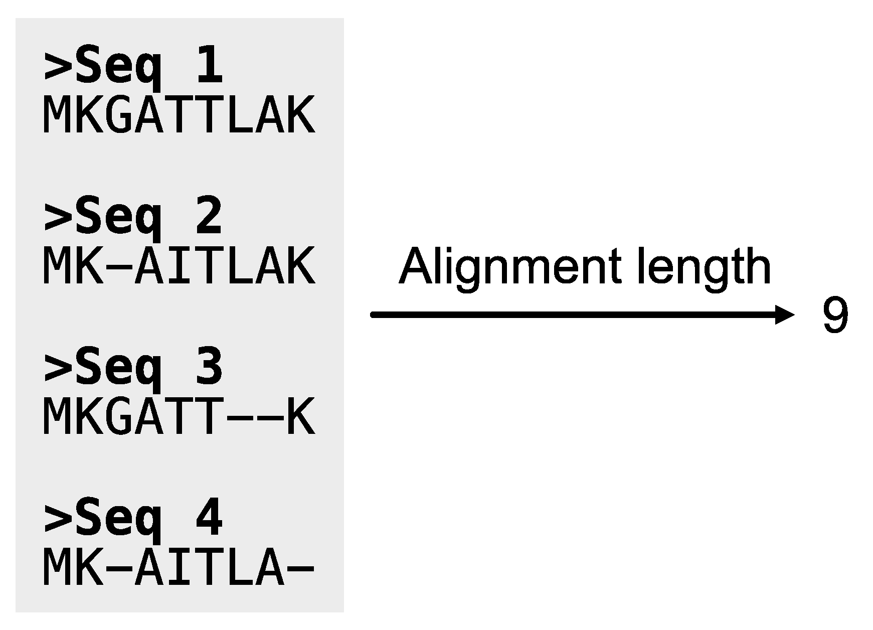
Figure 11. Calculating the length of alignments. The PhyKIT function aln_len can calculate the length of alignments.

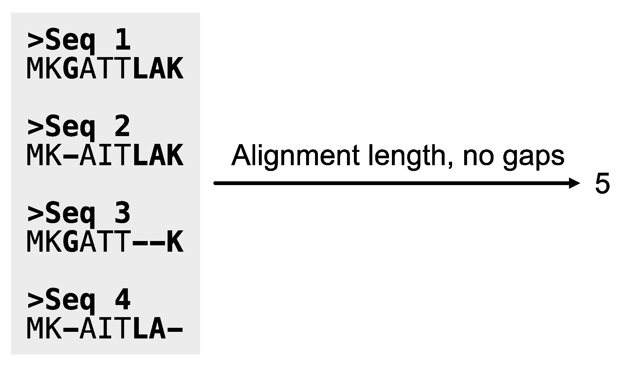
Figure 12. Calculating the length of alignments, excluding sites with gaps. The PhyKIT function aln_len can calculate the length of alignments. Sites in the alignment that contain a gap character are depicted in bold font.

Figure 13. Calculating pairwise sequence identities. Pairwise sequence identities can be calculated using the pairwise_id function. The output is summary statistics of sequence similarity for each pairwise comparison. Alternatively, users can use the –verbose option to output the sequence similarity between each pairwise comparison of sequences. Users can also exclude sites with gaps during pairwise identity calculations using the -e/--exclude_gaps function.

Figure 14. Determining the number and percentage of parsimony informative sites in an alignment. The PhyKIT function pis calculates the number and percentage of parsimony informative sites in an alignment. Here, the alignment of length nine has one site that is parsimony informative (denoted in blue).

Figure 15. Calculating the relative compositional bias of alignments. The function rcv calculates relative compositional biases in alignments. Low RCV values indicate lower compositional biases whereas higher values reflect greater biases.

Figure 16. Calculating the number and percentage of variable sites. The function variable_sites determines the number of variable sites in an alignment. In addition to the number of variable sites, the alignment length and percentage of variable sites are also printed.

Figure 17. Calculating tree-based measures of information content. (i) The function bipartition_support_stats calculates summary statistics for the support values in a phylogenetic tree. Here, bipartition support values are depicted in blue. This argument also has a verbose option that allows users to acquire the underlying distribution of values that were used to calculate summary statistics. (ii) Branch length information can be used to estimate the rate of gene evolutionary across a phylogeny. The function evo_rate can calculate the evolutionary rate of a gene. (iii) The function tree_len can calculate the sum of branch lengths in a phylogeny. (iv) Treeness is a measure of signal-to-noise wherein higher values indicate a greater signal-to-noise ratio. The function treeness can calculate treeness.

Figure 18. Cartoon depiction of saturation. Saturation occurs when the number of observed substitutions underestimates the number of real substitutions. As a result, a perfect one-to-one ration of observed substitutions and real substitutions would be indicative of data that lacks saturation.

Figure 19. Calculating degree of violation in the molecular clock. The degree of violation in the molecular clock is a helpful metric to identify genes that violate the molecular clock assumption. Phylogenies with low degrees of violation in the molecular clock will have broadly similar branch lengths (left), while phylogenies that violate the molecular clock will have highly variable branch lengths (right). The blue font corresponds to the branch lengths.

Figure 20. Three possible topologies for a rooted quartet. When conducting a polytomy test, PhyKIT examines if the three topologies occur in equal frequency among a set of single-locus phylogenies, which would be a signature of a polytomy; if not, there would be no signature of a polytomy. Polytomies may represent a lack of resolution at a particular internode or, given sufficient data, be a signature of a radiation event.

Figure 21. Exemplary phylogenies that do and do not display signatures of coevolution. Single gene phylogenies are depicted in blue or green. Phylogenies that have similar branch lengths across speciation events harbor a signature of coevolution (left). Phylogenies that do not have similar branch lengths are not coevolving (right).

Table 1. A complete list of PhyKIT functions as of version 1.19.0.

	Function Name	Function Alias(es)	Description
Alignment-based functions	alignment_length	aln_len; al	Calculate alignment length.
	alignment_length_no_gaps	aln_len_no_gaps; alng	Calculate alignment length excluding sites with gaps.
	alignment_recoding	aln_recoding; recode	Recode alignments using reduced character states.
	column_score	cs	Calculates column score. Column score is an accuracy metric for a multiple alignment relative to a reference alignment.
	compositional_bias_per_site	comp_bias_per_site; cbps	Calculates compositional bias per site in an alignment. Site-wise chi-squared tests are conducted in an alignment to detect compositional biases.
	create_concatenation_matrix	create_concat; cc	Create a concatenated alignment file. This function is used to help in the construction of multi-locus data matrices.
	evolutionary_rate_per_site	evo_rate_per_site; erps	Estimate evolutionary rate per site. Values may range from 0 (slow evolving; no diversity at the given site) to 1 (fast evolving; all characters appear only once).
	faidx	get_entry; ge	Extracts sequence entry from FASTA file.
	gc_content	gc	Calculate GC content of a FASTA file.
	pairwise_identity	pairwise_id; pi	Calculate the average pairwise identity among sequences. Pairwise identities can be used as proxies for the evolutionary rate of sequences.
	parsimony_informative_sites	pis	Calculate the number and percentage of parismony informative sites in an alignment.
	relative_composition_variability	rel_comp_var; rcv	Calculate RCV (relative composition variability) for an alignment. Lower RCV values are thought to be desirable because they represent a lower composition bias in an alignment.
	relative_composition_variability_taxon	rel_comp_var_taxon; rcvt	Calculate RCVT (relative composition variability, taxon) for an alignment. RCVT is the relative composition variability metric for individual taxa. Lower RCVT values are more desirable because they indicate a lower composition bias for a given taxon in an alignment.
	rename_fasta_entries	rename_fasta	Rename entries in a FASTA file. Note, the input FASTA file does not need to be a multiple sequence alignment.
	sum_of_pairs_score	sops; sop	Calculates sum-of-pairs score. Sum-of-pairs is an accuracy metric for a multiple alignment relative to a reference alignment.
	thread_dna	pal2nal; p2n	Thread DNA sequence onto a protein alignment to create a codon-based alignment.
	variable_sites	vs	Calculate the number and percentage of variable sites in an alignment.
Tree-based functions	bipartition_support_stats	bss	Calculate summary statistics for bipartition support.
	branch_length_multiplier	blm	Multiply branch lengths in a phylogeny by a given factor. This can help modify reference trees when conducting simulations or other analyses.
	collapse_branches	collapse; cb	Collapse branches on a phylogeny according to bipartition support. Bipartitions will be collapsed if they are less than the user specified value.
	covarying_evolutionary_rates	cover	Quantify the degree of coevolution between two single-gene trees.
	degree_of_violation_of_a_molecular_clock	dvmc	Calculate degree of violation of a molecular clock (or DVMC) in a phylogeny. Lower DVMC values are thought to be desirable because they are indicative of a lower degree of violation in the molecular clock assumption.
	evolutionary_rate	evo_rate	Calculate a tree-based estimation of the evolutionary rate of a gene.
	hidden_paralogy_check	clan_check	Scan tree for evidence of hidden paralogy. Specifically, this method will examine if a set of well-known monophyletic taxa are, in fact, exclusively monophyletic.
	internal_branch_stats	ibs	Calculate summary statistics for internal branch lengths in a phylogeny. Internal branch lengths can be useful for phylogeny diagnostics.
	internode_labeler	il	Appends numerical identifiers to bipartitions in place of support values. This is helpful for pointing to specific internodes in supplementary files or otherwise.
	last_common_ancestor_subtree	lca_subtree	Obtains subtree from a phylogeny by getting the last common ancestor from a list of taxa.
	long_branch_score	lb_score; lbs	Calculate long branch scores in a phylogeny. Lower long branch scores are thought to be desirable because they are indicative of taxa or trees that likely do not have issues with long branch attraction.
	monophyly_check	is_monophyletic	This analysis can be used to determine if a set of taxa are exclusively monophyletic. By exclusively monophyletic, if other taxa are in the same clade, the lineage will not be considered exclusively monophyletic.
	nearest_neighbor_interchange	nni	Generate all nearest neighbor interchange moves for a binary rooted tree.
	patristic_distances	pd	Calculate summary statistics among patristic distances in a phylogeny. Patristic distances are all tip-to-tip distances in a phylogeny.
	polytomy_test	polyt_test; polyt; ptt	Conduct a polytomy test for three clades in a phylogeny. Polytomy tests can be used to identify putative radiations as well as identify well supported alternative topologies.
	print_tree	print; pt	Print ASCII tree of input phylogeny.
	prune_tree	prune	Prune tips from a phylogeny.
	rename_tree	rename_tips	Renames tips in a phylogeny.
	robinson_foulds_distance	rf_distance; rf_dist; rf	Calculate Robinson-Foulds distance between two trees. Low Robinson-Foulds distances reflect greater similarity between two phylogenies. This function prints out two values, the plain Robinson-Foulds value and the normalized Robinson-Foulds value, which are separated by a tab.
	root_tree	root; rt	Roots phylogeny using user-specified taxa.
	spurious_sequence	spurious_seq; ss	Identifies potentially spurious sequences and reports tips in the phylogeny that could possibly be removed from the associated multiple sequence alignment. PhyKIT does so by identifying and reporting long terminal branches defined as branches that are equal to or 20 times the median length of all branches.
	terminal_branch_stats	tbs	Calculate summary statistics for terminal branch lengths in a phylogeny.
	tip_labels	tree_labels; labels; tl	Prints the tip labels (or names) a phylogeny.
	tip_to_tip_distance	t2t_dist; t2t	Calculate distance between two tips (or leaves) in a phylogeny.
	tip_to_tip_node_distance	t2t_node_dist; t2t_nd	Calculate distance between two tips (or leaves) in a phylogeny. Distance is measured by the number of nodes between one tip and another.
	total_tree_length	tree_len	Calculate total tree length, which is a sum of all branches.
	treeness	tness	Calculate treeness statistic for a phylogeny. Higher treeness values are thought to be desirable because they represent a higher signal-to-noise ratio.
Alignment- and tree-based functions	saturation	sat	Calculate saturation for a given tree and alignment. Saturation is defined as sequences in multiple sequence alignments that have undergone numerous substitutions such that the distances between taxa are underestimated.
Alignment- and tree-based functions	treeness_over_rcv	toverr; tor	Calculate treeness/RCV for a given alignment and tree. Higher treeness/RCV values are thought to be desirable because they harbor a high signal-to-noise ratio are least susceptible to composition bias.

Table 2. Recoding schemes available in PhyKIT.

Recoding Scheme Name	Nucleotides or Amino Acids	Description	Reference
RY-nucleotide	Nucleotides	Two characters; one character for purines and another for pyrimidines	(Phillips et al., 2004)
SandR-6	Amino Acids	Six characters; based on the JTT substitution matrix	(Susko and Roger, 2007)
KGB-6	Amino Acids	Six characters; based on the WAG substitution matrix	(Kosiol et al., 2004)
Dayhoff-6	Amino Acids	Six characters; based on the Dayhoff (or PAM250) matrix	(Embley et al., 2003)
Dayhoff-9	Amino Acids	Nine characters; based on the Dayhoff (or PAM250) matrix	(Hernandez and Ryan, 2021)
Dayhoff-12	Amino Acids	Twelve characters; based on the Dayhoff (or PAM250) matrix	(Hernandez and Ryan, 2021)
Dayhoff-15	Amino Acids	Fifteen characters; based on the Dayhoff (or PAM250) matrix	(Hernandez and Ryan, 2021)
Dayhoff-18	Amino Acids	Eighteen characters; based on the Dayhoff (or PAM250) matrix	(Hernandez and Ryan, 2021)
<file path>	Either	Custom recoding scheme specified using a two-column file. The first column is the recoded character and the second is the character in the alignment.	NA

Table 3. Summary of whether high or low values are desirable for phylogenomic subsampling.

Feature being subsampled	Metric for subsampling	PhyKIT function	Higher/Lower values are better
Taxa	Relative composition variability, taxon (RCVT)	relative_composition_variability_taxon; rel_comp_var_taxon; rcvt	Lower
Taxa or Gene	Long branch score	long_branch_score; lb_score; lbs	Lower
Gene	Alignment length	alignment_length; aln_len; al	Higher
	Alignment length, no gaps	alignment_length_no_gaps; aln_len_no_gaps; alng	Higher
	Pairwise identity	pairwise_identity; pairwise_id, pi	Context dependent
	Relative composition variability	relative_composition_variability; rel_comp_var; rcv	Lower
	Variable sites	variable_sites; vs	Higher
	Average (or median) bipartition support value	bipartition_support_stats; bss	Higher
	Evolutionary rate	evolutionary_rate, evo_rate	Context dependent
	Total tree length	total_tree_length; tree_len	Context dependent
	Treeness	treeness; tness	Higher
	Saturation	saturation; sat	Higher
	Treeness / Relative composition variability	treeness_over_rcv; toverr; tor	Higher
	Degree of violation of the molecular clock	degree_of_violation_of_a_molecular_clock; dvmc	Lower
Sites	Compositional bias	compositional_bias_per_site; comp_bias_per_site; cbps	Lower
Sites	Evolutionary rate	evolutionary_rate_per_site; evo_rate_per_site; erps	Lower

Disclaimer/Publisher’s Note: The statements, opinions and data contained in all publications are solely those of the individual author(s) and contributor(s) and not of MDPI and/or the editor(s). MDPI and/or the editor(s) disclaim responsibility for any injury to people or property resulting from any ideas, methods, instructions or products referred to in the content.

© 2024 by the authors. Licensee MDPI, Basel, Switzerland. This article is an open access article distributed under the terms and conditions of the Creative Commons Attribution (CC BY) license (http://creativecommons.org/licenses/by/4.0/).

Copyright: This open access article is published under a Creative Commons CC BY 4.0 license, which permit the free download, distribution, and reuse, provided that the author and preprint are cited in any reuse.

MDPI Initiatives

Important Links

Choose an area of interest and we will send you notifications of new preprints at your preferred frequency.

Disclaimer

PhyKIT: A Multitool for Phylogenomics

Abstract

Introduction

Operation System Requirements

Conventions

Background Knowledge

Protocol 1: Installing PhyKIT and Syntax for Usage

Installing PhyKIT

PhyKIT Syntax

Summary Statistics and the Verbose Option

Requesting New Functions

Protocol 2: Constructing a Phylogenomic Supermatrix

Data Acquisition

Orthology Inference

Multiple Sequence Alignment and Trimming

Constructing a Concatenated Supermatrix

Constructing a Dataset for Two-Step Coalescence

Protocol 3: Detecting Anomalies in Orthology Relationships

Hidden Paralogy and Clan Check

Spurious Homolog Detection

Protocol 4: Quantifying Biases in Phylogenomic Data Matrices and Related Measures

Measuring Bias at the Level of Taxa

Phylogenomic Subsampling Using the Information Content of Alignments

Phylogenomic Subsampling Using the Information Content in Phylogenetic Trees

Combining the Information Content in Alignments and Trees for Phylogenomic Subsampling

Subsampling for Time Tree Analysis

Measuring Bias at the Level of Sites

Protocol 5: Identifying Polytomies

Protocol 6: Gene-Gene Coevolution as a Genetic Screen

Commentary

Related Tools

Troubleshooting

Future Directions

Acknowledgements

Glossary

References

MDPI Initiatives

Important Links

Subscribe