Preprint
Article

An Efficient Transformer-CNN Network for Document Image Binarization

Altmetrics

Downloads

91

Views

27

Comments

0

A peer-reviewed article of this preprint also exists.

This version is not peer-reviewed

Submitted:

22 April 2024

Posted:

25 April 2024

You are already at the latest version

Alerts
Abstract
Color image binarization plays a pivotal role in image preprocessing work, significantly impacting subsequent tasks, particularly in text recognition. This paper concentrates on Document Image Binarization (DIB), aiming to separate a image into foreground (text) and background (non-text content). Through a thorough analysis of conventional and deep learning-based approaches, we conclude that prevailing DIB methods leverage deep learning technology. Furthermore, we explore the receptive fields pre- and post-network training to underscore the Transformer model's advantages. Subsequently, we introduce a lightweight model based on the U-Net structure, enhanced with the Mobile ViT module to better capture global information features in document images. Given its adeptness at learning both local and global features, our proposed model exhibits superior performance on two standard datasets (DIBCO2012 and DIBCO2017) compared to state-of-the-art methods. Notably, our proposed DIB method presents a straightforward end-to-end model devoid of additional image preprocessing or post-processing. Moreover, its parameter count is less than a quarter of the HIP'23 model, which achives best results on three datasets(DIBCO2012, DIBCO2017 and DIBCO2018). Finally, two sets of ablation experiments were conducted to verify the effectiveness of the proposed binarization model.
Keywords: 
Subject: Computer Science and Mathematics  -   Artificial Intelligence and Machine Learning

1. Introduction

Document Image Binarization (DIB) is one of the crutial image preprocessing works, and is applied as a basic approach for image processing, such as text recognition [1,2,3,4,5], feature extraction [6] and so on. A well preprocessed binarized image has significant effect on the results of Optical Charactor Recognigion (OCR) [7]. The goal of DIB is to separate the image into foreground (text) and background (non-text content). The foreground pixel value is 0 and the background pixel value is 255, which is what we usually call "black words and white paper".
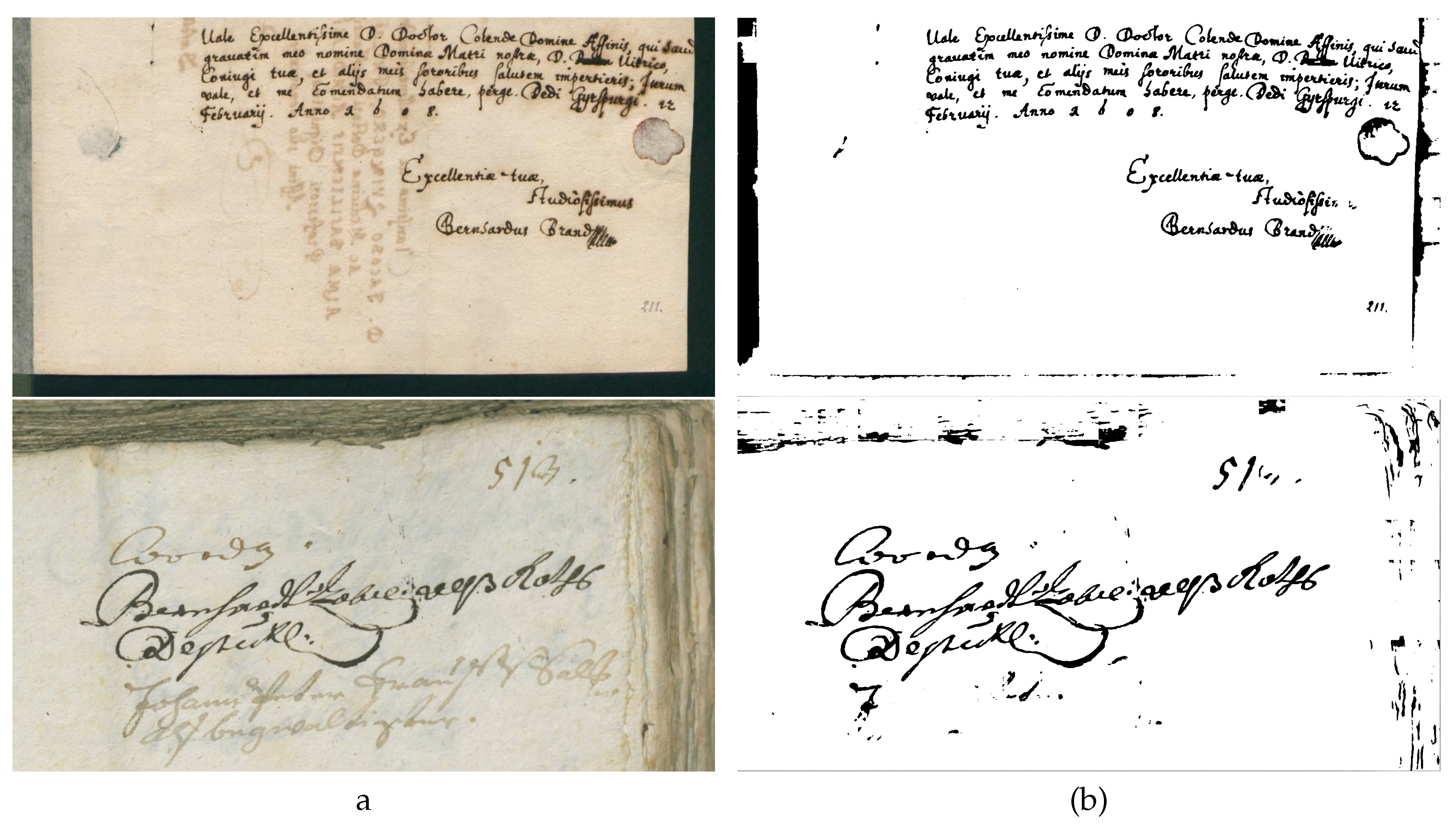
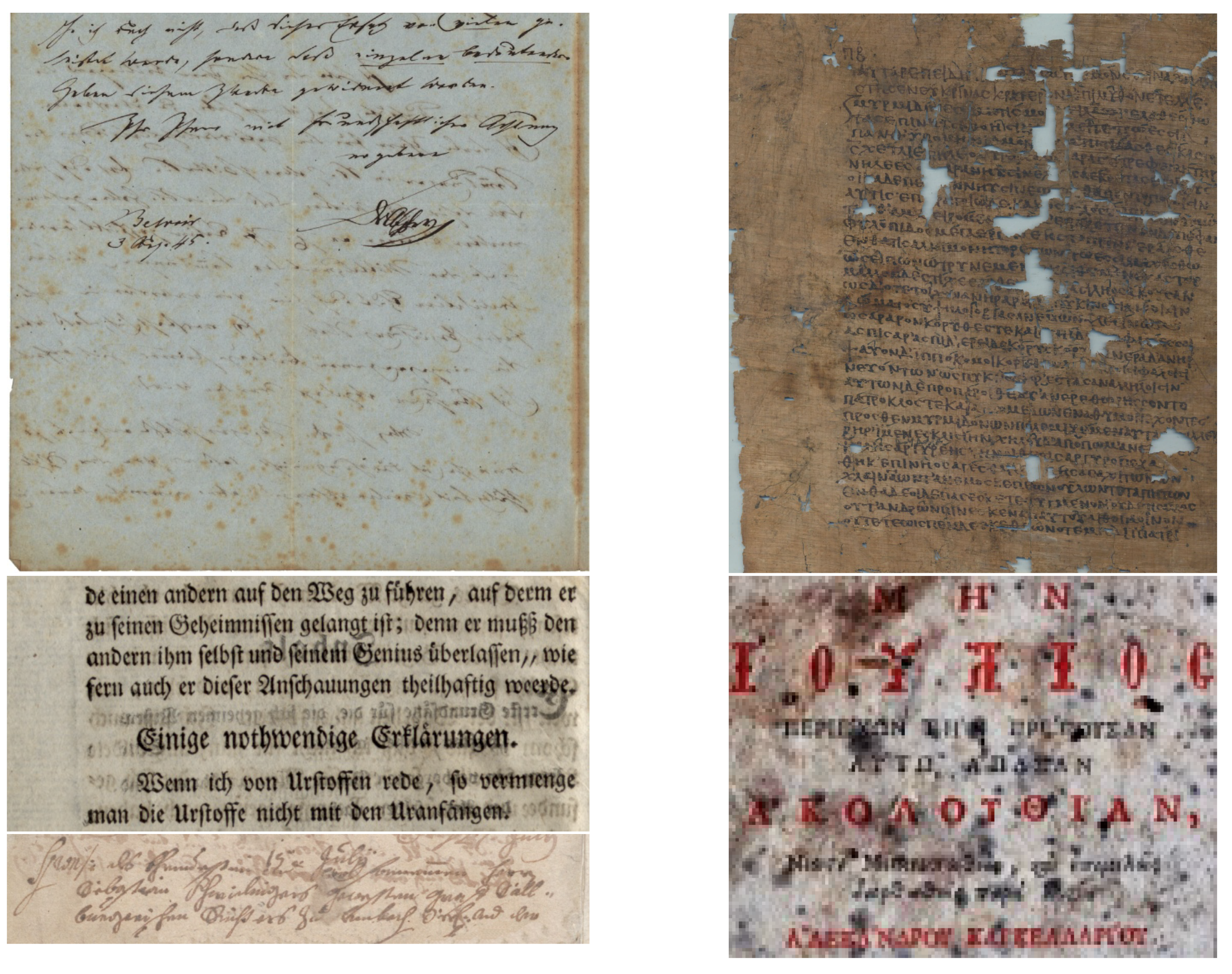
The document images like the ancient text data, always suffered serious degradations as shown in Figure 1 and Figure 2. These images are from the datasets of the International Frontiers in Handwriting Recognition Conference, which started in 2009 and held almost every year [8,9,10,11,12,13,14,15,16,17,18]. Document image binarization holds substantial practical application value and significance in this regard. The digital processing of degraded documents is a crucial method for addressing challenges in historical document preservation and cultural heritage conservation. Manual processing of large volumes of historical text materials entails significant time and labor, and is susceptible to errors. Therefore, employing computers for automatic processing of images of ancient text materials is imperative.
As depicted in Figure 1 and Figure 2, various textual issues are evident in the document images. For instance, Figure 1 illustrates text inconsistencies such as variations in texture, font size, and color, alongside distortions in the alignment of text content lines, yellowing of paper, and ink contamination. Similarly, Figure 2 showcases damaged and incomplete textual elements, significant blurring, and the presence of strong background textures causing interference within the text area. In summary, the analysis and recognition of textual information within handwritten document images of ancient books or early printed materials pose formidable challenges. Therefore, research into document image binarization for text segmentation holds particular significance.
Many approaches have been proposed to realize document image binarization. The typical methods include thresholding methods, such as the Otsu algorithm [20], Niblack’s method [21], Sauvola’s method [22], Wolf’s method [23], among others [24,25,26,27,28,29,30,31,32,33,34,35]. There are also other traditional algorithms based on edge detection [36,37,38,39,40], and others utilizing fuzzy logic [41,42,43,44,45]. Additionally, there is one method, the winner of DIBCO2018 [46].
In recent years, the achievements in document image binarization research have primarily been realized through deep learning [19,47,48,49,50,51,52,53,54,55,56,57,58,59,60,61,62,63]. Neural networks have demonstrated remarkable ability to segment foreground text and background of document images, as demonstrated by a comparison of the deep learning algorithm [63] with the traditional method [46] (winner of DIBCO2018) for binarization of handwritten document images, as shown in Figure 3.
From Figure 3, it is evident that Rezanezhad et al. [63] segmented the foreground text and the most prominent background textures. Their model attained the top performance across three document image datasets (DIBCO2012, DIBCO2017, and DIBCO2018) at the 2023 International Symposium on Imaging and Processing Historical Documents. The model is based on the U-Net structure and the locally applied transformer, which has significant segmentation capability. Based on the further research and analysis of their model, we propose a new model of document image binarization with fewer parameters and better performance.
This paper introduces a novel model that combines the U-Net architecture with Transformer, integrating Mobile ViT for document image binarization for the first time. The main contributions of this paper are as follows:
We have discussed the characteristics of different types of deep learning methods for document image binarization and have also illustrated the receptive fields of the CNN and Transformer models.
By incorporating the Mobile ViT block into the U-Net structure, we aim to broaden the receptive fields of the image, capturing both global and local characteristics more effectively. This marks the first application of Mobile ViT in document image binarization. The parameters of the proposed model are only one-fourth of those of a similar model [63] based on U-Net for document image binarization.
MVT-Unet is a straightforward end-to-end model trained only once, without employing pre- or post-processing steps or ensemble methods.
MVT-Unet demonstrates superior performance compared to state-of-the-art results on two standard Document Binarization Competition (DIBCO) datasets, for both handwritten and machine-printed documents.
The paper is structured as follows. In section 2, we review various document image binarization methods. Section 3 discusses the proposed model. We present the experimental results and comparisons with other approaches on several DIBCO datasets in section 4. Section 5 showcases two sets of ablation experiments on the core modules of the proposed model. Finally, section 6 concludes the paper.

2. Related Work

In this section, we overview the different algorithms or models for ducoment image binarization and analysis the characteristics of each methods. It is well known that, many approaches have been proposed to address this issue. These techniques can be roughly categorized into traditional approaches [20,21,22,23,24,25,26,27,28,29,30,31,32,33,34,35,36,37,38,39,40] based on edge detection, [41,42,43,44,45] using fuzzy logic other kinds like [46] and deep learning methods [19,47,48,49,50,51,52,53,54,55,56,57,58,59,60,61,62,63,64,65,66,67,68,69,70,71].

2.1. Traditional Binarization Techniques

The Otsu algorithm, pioneered by Otsu [20], stands as one of the most renowned thresholding methods for document image binarization. It endeavors to ascertain an optimal threshold value through comprehensive grayscale image analysis. However, its single threshold approach proves inadequate for handling low-contrast or unevenly illuminated images. Consequently, alternative methodologies have been proposed to mitigate the limitations inherent in employing a fixed threshold. Noteworthy among these are Niblack [21], Sauvola [22], Wolf [23], and others [24,25,26,27,28,29,30,31,32,33,34,35].
Recognizing the significance of stroke continuity, particularly in degraded handwritten document images, Holambe et al. [39] introduced a methodology integrating contrast mapping with Canny’s edge detection, aimed at identifying text stroke edge pixels. Subsequently, thresholding techniques are applied to delineate background and foreground regions. Similarly, conventional algorithms [36,37,38,39,40] predominantly rely on edge detection for document image binarization. Numerous other traditional approaches [42,43,44,45,46] have been proposed in pursuit of achieving optimal document image binarization.
Among these, the work of Xiong et al. [46] merits attention as the victor of the 2018 Document Image Binarization Competition. This method exemplifies a conventional approach that leverages background estimation and Laplacian energy segmentation techniques exclusively for document image binarization. Despite its accolades, limitations become evident, particularly when the image is afflicted by similar background textures and text, as illustrated in Figure 3(c).

2.2. Deep Learning Binarization Approaches

As we can seen the binarization result of the document image obtained by Rezanezhad et al. [63] in Figure 3(d), it is almost well segmented the text information in the original document image. Even the binarization result of Rezanezhad et al. [63] still has some areas that are not well segmented. For example, the background information far away from the text information is incorrectly classified as foreground. But it can also be clearly seen that the results of document image binarization based on deep learning are far better than those of traditional methods, so the algorithms of document image binarization in the past three years are basically studied on the technology of deep learning. Such as literature [57,58,59,60,61,62,63,66,67,68,69,72,73].
The models of document image binarization based on deep learning technology are mainly divided into two research directions. One is the model obtained based on Convolutional Neural Network (CNN) [19,47,48,49,50,51,52,53,54,55,56,57,58,59,60,61,62,63], and the other is based on Generative Adversarial Networks (GANs) [66,67,68,69].
Calvo and Gallego [19] use of convolutional auto-encoders devoted to learning an end-to-end map from an input image to its selectional output through the activation functions to indicate the pixels to be either foreground or background. This model is once trained, and outperform the existing binarization strategies in the same period. While it is not as good as Rezanezhad et al. [63], which is the U-Net based structure with adding attention mechanism (Transformer). The detailed comparison of these two modesl and the reasons will explained in the next section. Other CNN-base models [48,49,51,53,55,64,65,66,67,68,69,70,71,72,74] or using U-Net structure models [52,54,56,62,73] are developed in the past years.
Generative Adversarial Networks (GANs) [75] include generator networks and discriminator networks. Souibgui et al. [66] apply conditional generation adversarial networks (cGANs) to develop an Document Enhancement Generative Adversarial Networks (DE-GAN) to restore severely degraded document images, including the binarization task. They input a degraded image with its Ground Truth (GT) to the discriminator, which forces the generator to generate an output that is indistdistinguishable from the GT. After training, the discriminator becomes unnecessary and only the generator network is used to enhance the degraded image. Differently, Rajesh et al. [70] employ the Dual Discriminator Generative Adversarial Network (DD-GAN) [65] to achieve binarization directly using JPEG compressed stream of document images. Others GAN-based models [64,67,70,71] are constructed to realize the binarization issure.
In summary, the above CNN-based models [19,47,50,57,58,59,60,61] generally have the advantages of CNN, simple structure design, fewer parameters, and high computational efficiency, especially friendliness to limited computing resources. While the models [64,65,66,67,68,69,70,71] operating within the GAN framework have the characteristics of GANs. Through the unsupervised generative model, on the basis of a well-trained discriminator, it can produce clearer and more realistic sample results. Nevertheless, GANs also suffer from certain drawbacks, such as mode collapse and mode shock in the training process, which may lead to the unstable quality or lack of diversity of the generated document image. GAN training procedures are typically intricate and necessitate meticulous design and parameter tuning, often requiring considerable time investment to achieve desired outcomes.

3. Methodology

3.1. Baseline Network for Document Image Binarization

Based on the above analysis and summary of the document image binarization task using CNN and GAN, we found that the essence of the document image binarization work is the segmentation task of the target image (that is, the segmentation of the foreground text and the background). U-Net network was proposed by Olaf et al [76] in 2015, which is used for medical image segmentation tasks and has achieved excellent results. Due to its excellent performance on segmentation tasks, this structure has attracted the attention of binarization related research. There are several U-Net based document image binarization methods [54,63,77,78]. Because U-Net has two advantages, one is the simple left-to-right symmetric convolution model, the other is the skip connection. The first point is the essence to realize the process of encoding and decoding through pure convolution, downsampling and upsampling, these are the process of compressing the image features, retaining only the key information, and restoring the image, ensuring that the output image is consistent with the size of the input image. The second point is that the a skip connection in the process of encoding and decoding, makeing the features at the pixel level of the image and the semantic features are fused, and this feature fusion of different scales is very beneficial for the recovery of the image through upsampling. Therefore, U-Net network can do semantic segmentation at the pixel level, so it is very suitable for the segmentation task of text and background of document images. In addition, U-Net has the advantage that it can learn well even with a small amount of labeled data through the use of data augmentation and special network architecture, which is very suitable for datasets with a small amount of labeled document images.
In short, pure convolutional networks can be easily adjusted and optimized according to different task requirements due to their simple structure design, and adapt to various sizes and types of image processing tasks, which U-Net has, while pure cascaded convolutional neural networks cannot achieve the structure designed by U-Net due to its symmetric structure and skip connections. It can transfer information between different levels of the network, can fuse feature maps of different resolutions, and effectively combine depth and context information in order to retain more detailed information, so as to achieve better document image binarization effect.
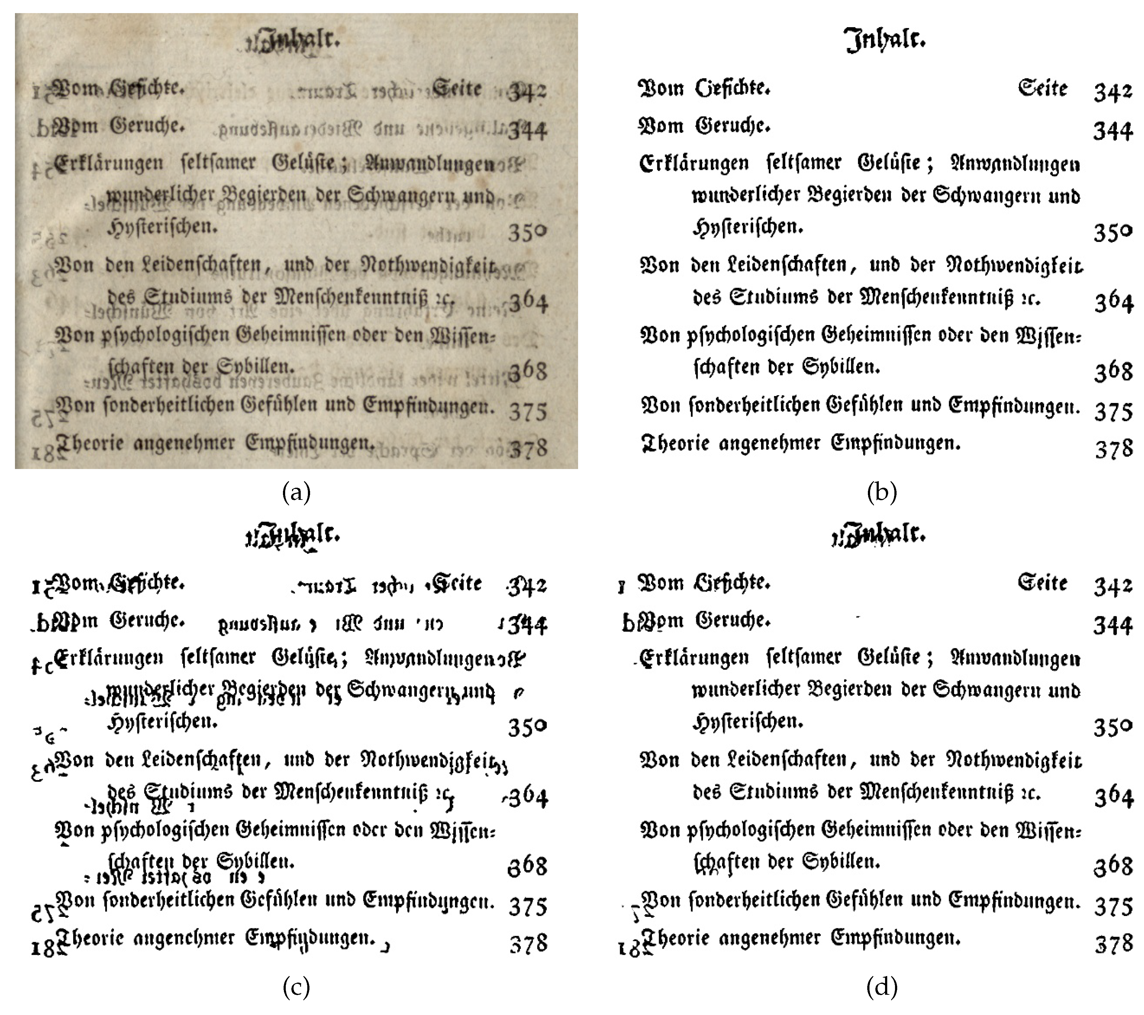
Because of the advantages of convolution and U-Net network, we will conduct experimental exploration on the document image binarization model [19] and the pure U-Net model. However, we found problems in several cases, as shown in Figure 4. In Figure 4, the binarization results presented in (c) and (d) show that the textural background information similar to photocopied content and text information in the original document image cannot be segmented reasonably. However, the original document image of Figure 4(a) is severely polluted, and even the texture in the background has strong contrast. Relying only on simple cascaded convolution or U-Net network training cannot fully capture the overall features and achieve the "black and white" binarization effect we want. This problem mainly stems from the limitation of receptive field range, that is, simple cascade convolution and U-Net network are difficult to learn a wider range of receptive field features.

3.2. Improving Network Receptive Field Range

In the previous subsection, we mentioned the concept of receptive field, let’s first briefly introduce this concept. The receptive field in a biological neural network is the input region that the neuron “sees”, while in a deep learning convolutional neural network, the computation of an element in the feature map is affected by a region of the input image, which is the receptive field of that element. There are two ways to calculate the receptive field specifically. A began to calculate step by step input layer [79], typical calculation formula formula such as l k = l k 1 + ( f k 1 ) i = 1 k 1 s i , l k , f k , s k represents the receptive field, kernel size and step size of the klayer, respectively. Another approach, proposed by Luo et al. [80], uses backpropagation to compute the “effective receptive field”. In their literature, the effective receptive field is defined as the region of input pixels that have some influence on the central output unit. By analyzing the distribution of the effective receptive field with different weights, they deduced the mathematical characteristics of the effective receptive field in the general case involving nonlinear activation functions, which were calculated by the main formulas (1) and (2). And the variance formula (3) and expectation (4).
l x i , j 0 = i , j l y i , j y i , j x i , j 0
Where lis the loss function, the pixels of each layer are indexed by ( i , j ) and its center is ( 0 , 0 ) . Where x i , j 0 for the network’s input, y i , j = x i j n for the first nlayer of output, the purpose is to want to measure each xto y contribution.
g ( i , j , p 1 ) = σ i , j p a = 0 k 1 b = 0 k 1 w a , b p g ( i + a , i + b , p )
Where g(I, j, p) for the first player gradient, σ i , j p for the first player on pixel ( i , j ) activation function gradient, w a , b p is the convolution kernel layer in p ( a , b ) convolution weights.
V a r [ g ( i , j , p 1 ) ] = E [ σ i , j p 2 ] a = b V a r [ [ w a , b p ] V a r [ g ( i + a , i + b , p ) ] = 0
E [ σ i , j p 2 ] = V a r [ σ i , j p 2 ] = 1 / 4
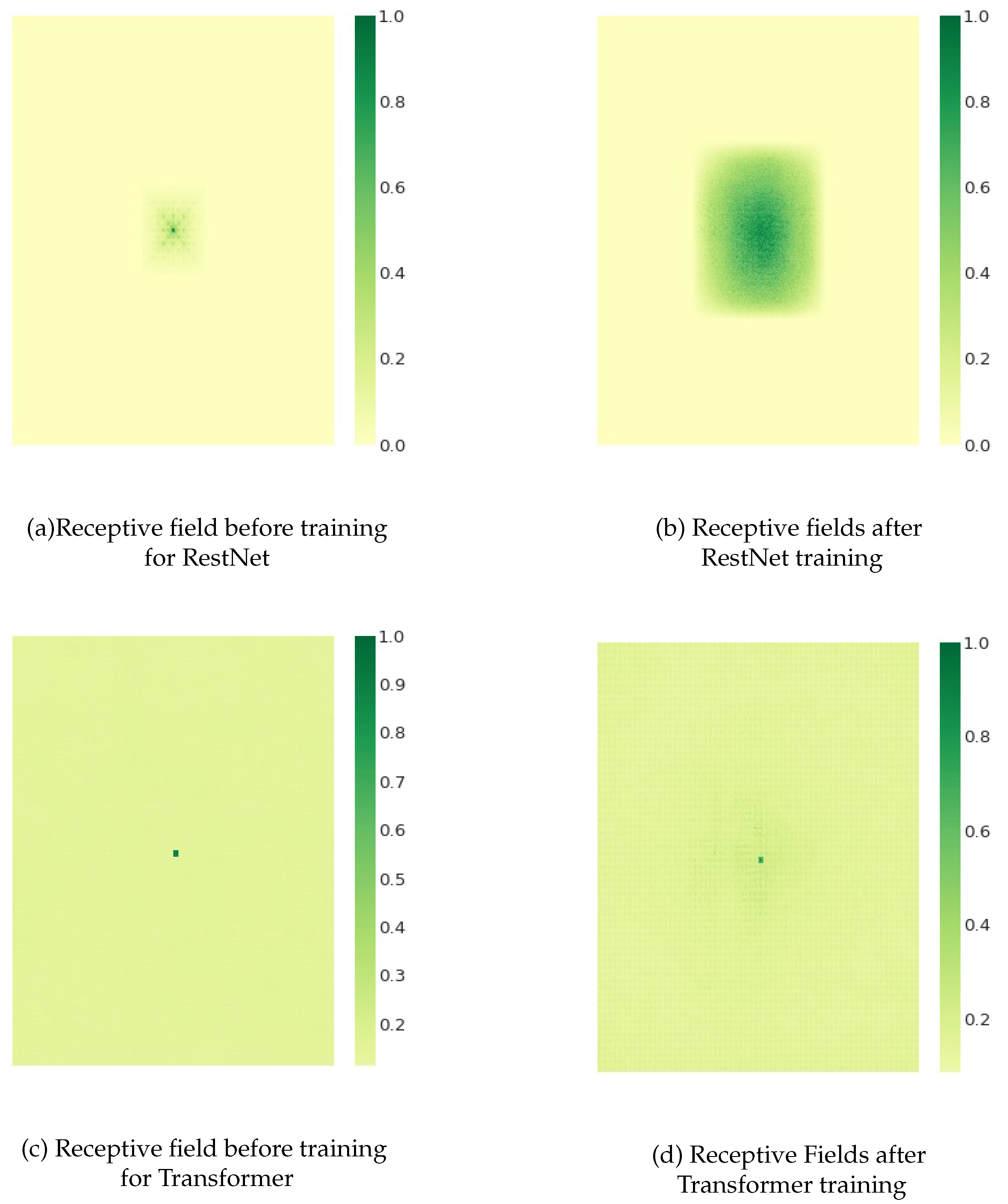
We use the effective receptive field calculation method proposed by Luo et al. [80], and plot the receptive field of a representative RestNet and Transformer before and after training in Figure 5. From the comparison effects of Figure 5(c)(d), it can be clearly seen that after Transformer training, the receptive field range of the central element covers almost the entire image, which is significantly better than the effect of ResNet (pure convolution)(the larger the value, the stronger the influence). This shows that the model of the Transformer architecture can effectively deal with long-distance dependencies through the self-attention mechanism, so that the model can better understand the association between distant locations, so as to better capture the global dependencies. In addition, the flexibility and versatility of the Transformer architecture makes it suitable for various computer Vision tasks (Vision Transformers, or Vits), and it is their powerful modeling capabilities that allow their architectural form to flourish.
In 2021, the Mobile ViT model proposed by Sachin and Mohammed upcite 2021MobileViT is a lightweight Vision Transformer architecture. The model architecture of Mobile ViT is also explained in detail in Chapter 2 of this paper. The core components of the model are MV2 and Mobile ViT block, which makes it a fusion of the advantages of CNN and Transformer attention mechanisms. The most important module Mobile ViT block has the advantage of flexibly combining global self-attention and local feature extraction, and has the following four advantages in balancing performance and computing efficiency. The first is its lightweight structure, which makes it suitable for mobile devices with limited computing resources. The second is hierarchical feature extraction. The Mobile ViT block contains multiple sub-layers, which can effectively extract features of different abstract levels of the image. The third is cross-layer connection. Because it introduces a horizontal connection or jump connection mechanism, it is conducive to improving the efficiency and accuracy of feature transfer. Finally, the multi-scale processing feature can support inputs of different scales (i.e. input images of different sizes). These advantages make the Mobile ViT model perform well in balancing performance and computing efficiency.

3.3. Proposed Model

Just as the advantages of Mobile ViT block mentioned above, we introduce Mobile ViT block under U-Net architecture to build a document image binarization model. This study draws on the successful experience of Rezanezhad et al. [63] in the field of document image processing. Their model was featured in the 2023 International Symposium on Imaging and Processing of Historical Documents, in particular at DIBCO2012 [11], The best results were achieved on three datasets: DIBCO2017 [15] and DIBCO2018 [16]. With traditional algorithms [20,22,46] and other deep learning-based models [49,59,64,69,81], the model showed obvious advantages in visual effect and four commonly used indexes. One of the biggest advantages of the model [63] is the low requirement of graphics card resources and short training time. Using only an Nvidia 2080 graphics card, you can train a suitable document image binary model in two days. In addition, the model has a relatively small number of parameters, is based on the U-Net architecture, and the attention mechanism of Transformer is cleverly added at the bottom right side.
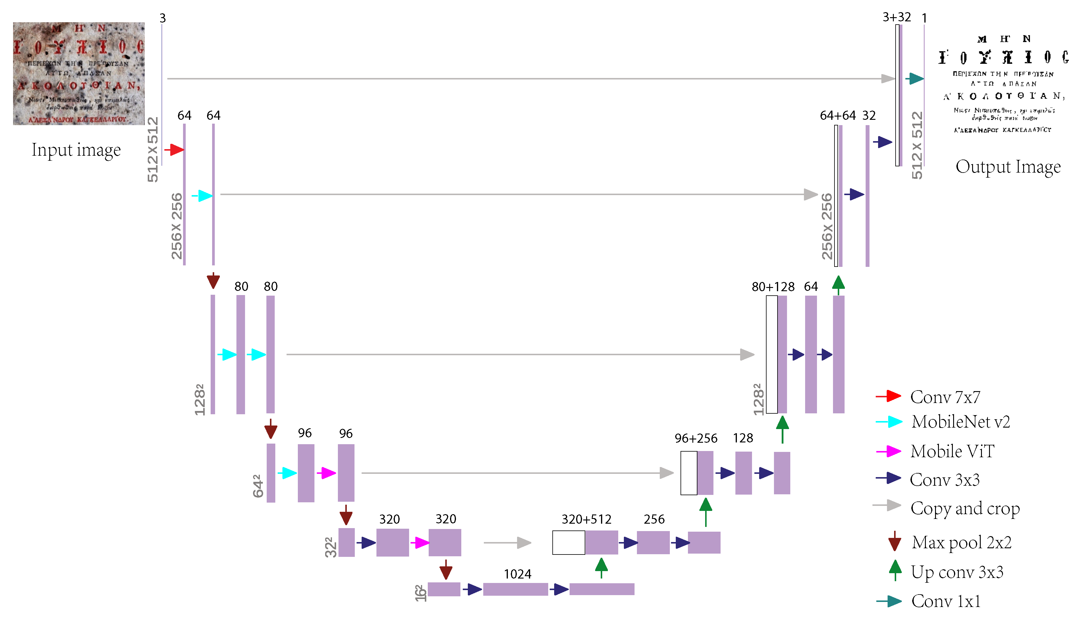
However, the Transformer structure in Rezanezhad et al. [63] model is used only after several convolution subsampling encodations, which results in insufficient learning of the overall structure information of the original image, as shown in Figure 4. In contrast, the model proposed in this study takes advantage of the lightweight advantages of Mobile ViT block to effectively learn the information features of document images during each convolution expansion process. This allows the model in this study to better integrate global and local image features. The overall structure of the document image binarization model in this study is shown in the figure. Due to the portability advantage of Mobile ViT block, the number of model parameters in this study has been greatly reduced, specifically by about 76% (the number of model parameters in this paper is 8923370, while the number of model parameters in Rezanezhad et al. [63] is 36980426). This makes the model studied in this paper more suitable for lightweight hardware devices.

4. Experiments and Analysis

In this section, we give the specific operation process of the experiment in detail, mainly including the experimental description, the qualitative analysis and quantitative analysis of the experimental results. In the following, we will introduce the specific details of the three parts in turn.

4.1. Introduction of Experiments

This part introduces the preparation work before model training. In order to objectively evaluate the performance of our proposed model, we used the same data set as that of Rezanezhad et al. [63] for experimental training. To be specific, We used the recent DIBCO dataset [8,9,10,11,12,13,14,15,16], the Bali Palm Leaf dataset [82] and the PHIBC [83] dataset of the Persian Heritage document image Binarization Competition.
For comparative experimental analysis, we selected DIBCO2012 [11], DIBCO2017 [15]DIBCO 2018 [16] as validation data set. The rest of the data set serves as the training data set, This is consistent with the model of Rezanezhad et al [63] and others [49,59,64,69,81] is consistent.
The training image size, learning rate, and number of epochs for our document image binarization model were all tuned through extensive experiments. The specific training process of the model was divided into two stages. In the first stage, the images of the training dataset were not cut, so as to learn the model from the overall structural features, and the complete image information after data enhancement processing was used for training, and the training epoch was set to 30. The second stage focuses on the learning ability of local detail information. In this stage, the original document image is diced, which results in the amount of training data increasing to more than four times that of the first stage, so the training epoch is set to 20.
The loss function for training document image binarization models is often the F-measure (FM), as described in [19,63]. The F-measure (FM) of an image, which is defined as the formula (5).
F M = 2 × P r e c i s i o n × R e c a l l P r e c i s i o n + R e c a l l
Where P r e c i s i o n = T P F P + T P , R e c a l l = T P F N + T P , and the three quantities T P , F P , F N respectively indicate that the experiment obtained correct positive values (the pixels in the foreground of the text were correctly divided into text). False positive values (pixels of the background are incorrectly classified as text foreground), and false negative values (text foreground is incorrectly classified as background). During our training, we set the foreground pixel value to 1 (" positive ") and the background pixel value to 0 (" negative ") in the true binary label (GT). Putting the calculation of P r e c i s i o n and R e c a l l into the formula (5), the simplified objective function can be obtained as follows.
F M = 2 T P 2 T P + F P + F N
An important problem in model training is the insufficient amount of training data. This is because the recent DIBCO datasets [8,9,10,11,12,13,14,15,16,17] only 11 datasets containing a total of 146 pairs of original document images and their true binarized label images (GT), Together with the 50 pairs of Bali palm leaf dataset [82] and the 16 pairs of images and their GT of PHIBC dataset [83], there are only 212 valid image pairs and labels in total. If the training target is DIBCO2017 dataset [15], only 172 pairs of images and their GT can actually be used for training (20 pairs without DIBCO2017 [15], and 20 pairs without DIBCO2017 [15]). It also does not contain the 20 pairs of DIBCO2019 [17], because the document image of this dataset is more complex, the degree of pollution type and the characteristics of the text are very different from those shown in other datasets. And other models for comparison [49,59,63,64,69,81] is trained without any data [15,17]). This is not sufficient for neural network model training, so similar to Rezanezhad et al. [63], We applied data augmentation to an existing dataset [60,84], including image rotation, scaling, brightness adjustment, and image chunking. In the specific training process, we trained DIBCO2012 [11], DIBCO2017 [15] and DIBCO2018 [16]. An input image size of 512 × 512 was chosen. The training process is divided into two stages, the first stage is a learning rate of 1e-3 or 8e-4 (depending on the training curve and the results), and the second stage uses a learning rate timer, the learning rate is halved every five iterations, and the initial learning rate is the same size as in the first stage.
In summary, through the comparative analysis of experimental results, the binarization model of document image proposed in this paper, We get better results on DIBCO2012 [11] and DIBCO2017 [15] datasets (compared to Rezanezhad et al. [63]). That is, it performs better in the four indicators of document image binarization. The results on the DIBCO2018 [16] dataset are not very good and we analyze this. In addition, this paper also conducts verification and comparison experiments on the DIBCO2019 [17] dataset (because the images of this dataset are severely damaged and the image features are different from the training dataset). It outperforms [63] and other traditional methods with the same parameters. In the following, we will analyze and discuss the experimental results through qualitative and quantitative aspects.

4.2. Qualitative evaluation

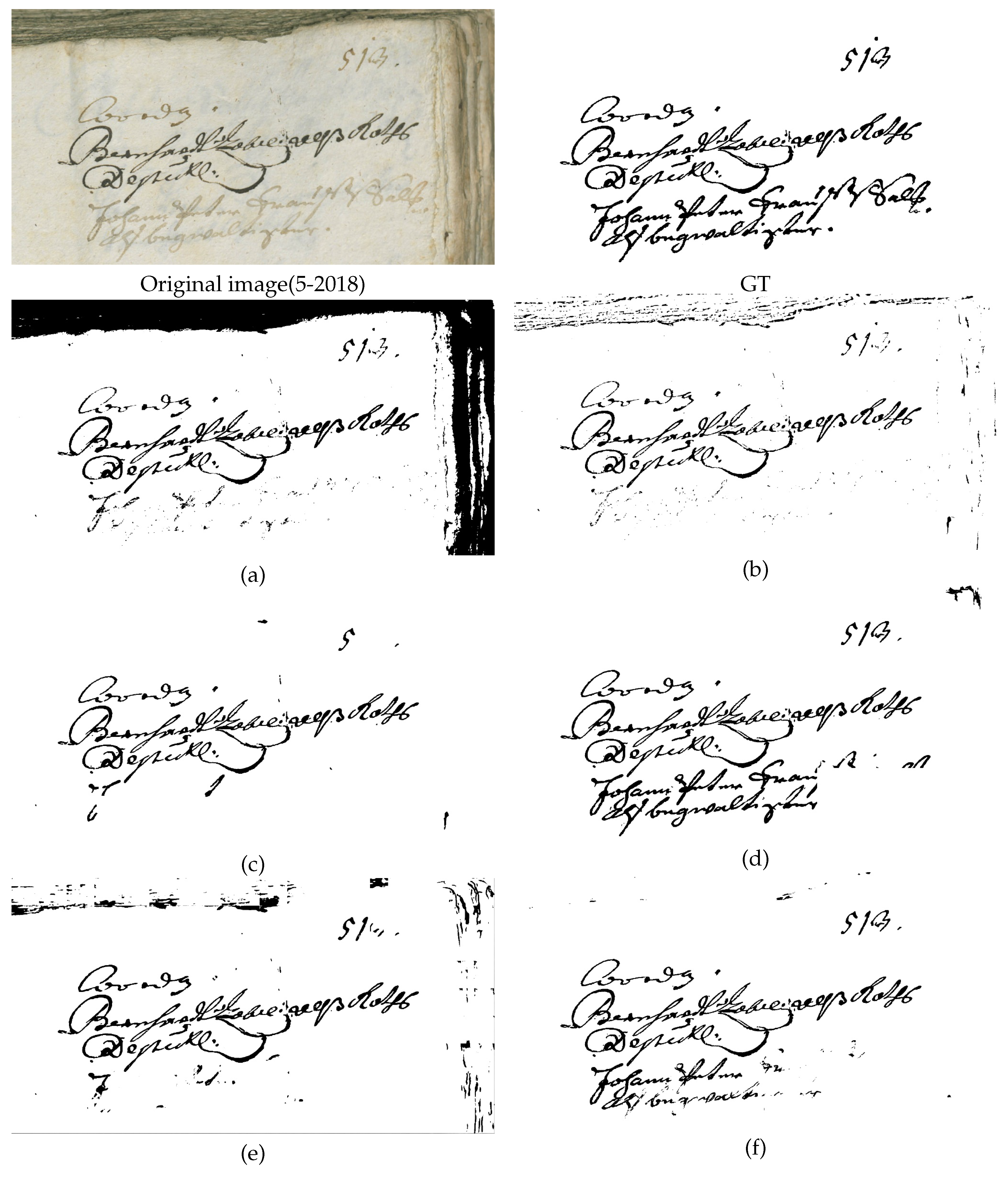
The experiments in this paper are compared and analyzed on DIBCO2012 [11], DIBCO2017 [15] and DIBCO2018 [16] datasets respectively. We compare the document image binarization model proposed in this paper with the deep learning-based model [49,59,63,64,69,81] and the classic traditional method [20,22,46] are compared on the three datasets [11,15,16]. By enumerating the visual comparison maps of the binarization results and calculating the relevant evaluation indicators, the comparative analysis is carried out. First, we show the visual comparison of different methods on different datasets in the Figure 7, Figure 8, Figure 9, Figure 10, Figure 11 and Figure 12.
From Figure 7, we can clearly see that Otsu [20] cannot distinguish the pollution in the second line of the original article image from the text content very well. This is mainly because the method is based on a global threshold. However, the traditional method Sauvola [22], which is based on local threshold, can basically separate the polluted background content from the text. Xiong et al. [46] method (as the champion algorithm of DIBCO2018 [16]) also cannot perfectly segment the text information in the thick area of the stroke, which indeed illustrates the limitations of the traditional binarization method. The model of Calvo and Gallego [19] is a simple cascade convolutional network. Obviously, it is found that its binarization results cannot distinguish well the features in the background far from the text area, so that there is a lot of noise in the result map. This shows that the pure convolution model indeed has a strong ability to learn only local features. The results of Rezanezhad et al. [63] do not perfectly extract only some of the thinner strokes and the sliding lines of the last two letters, and the rest of the text is almost completely separated from the background content.
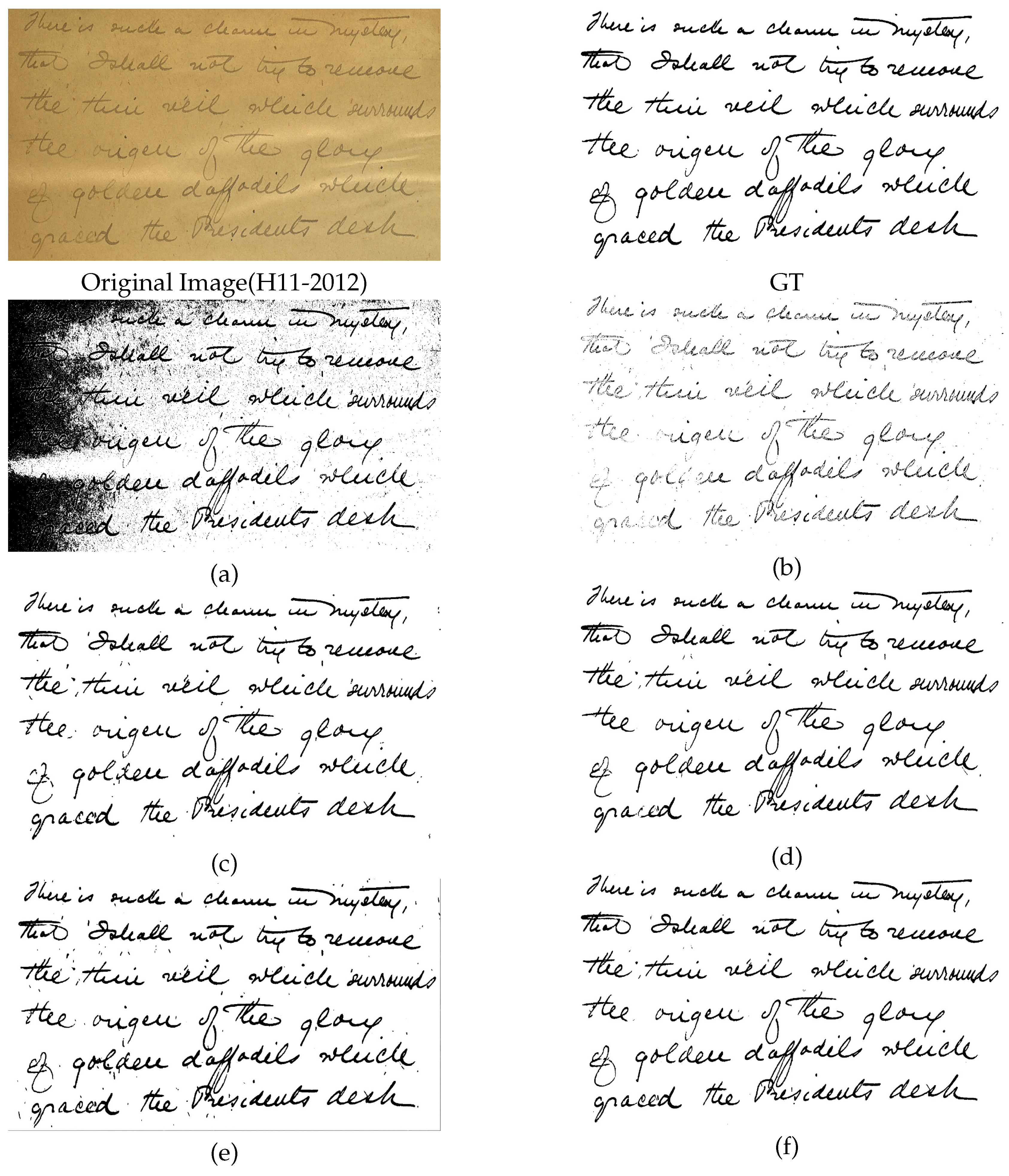
We can see from Figure 8 that the traditional methods based solely on global or local thresholds Otsu [20] and Sauvola [22], The result of binarization for the document image with uneven illumination is not very satisfactory. However, because Xiong et al [46] method estimates the overall background of the image and uses a variety of processing techniques, this kind of uneven illumination document image can also get better binarization results. At this point, the deep learning based models Calvo and Gallego [19] (just without the fully clean separation of background content), Rezanezhad et al [63]’s model and our model have achieved satisfactory binarization results for document images.
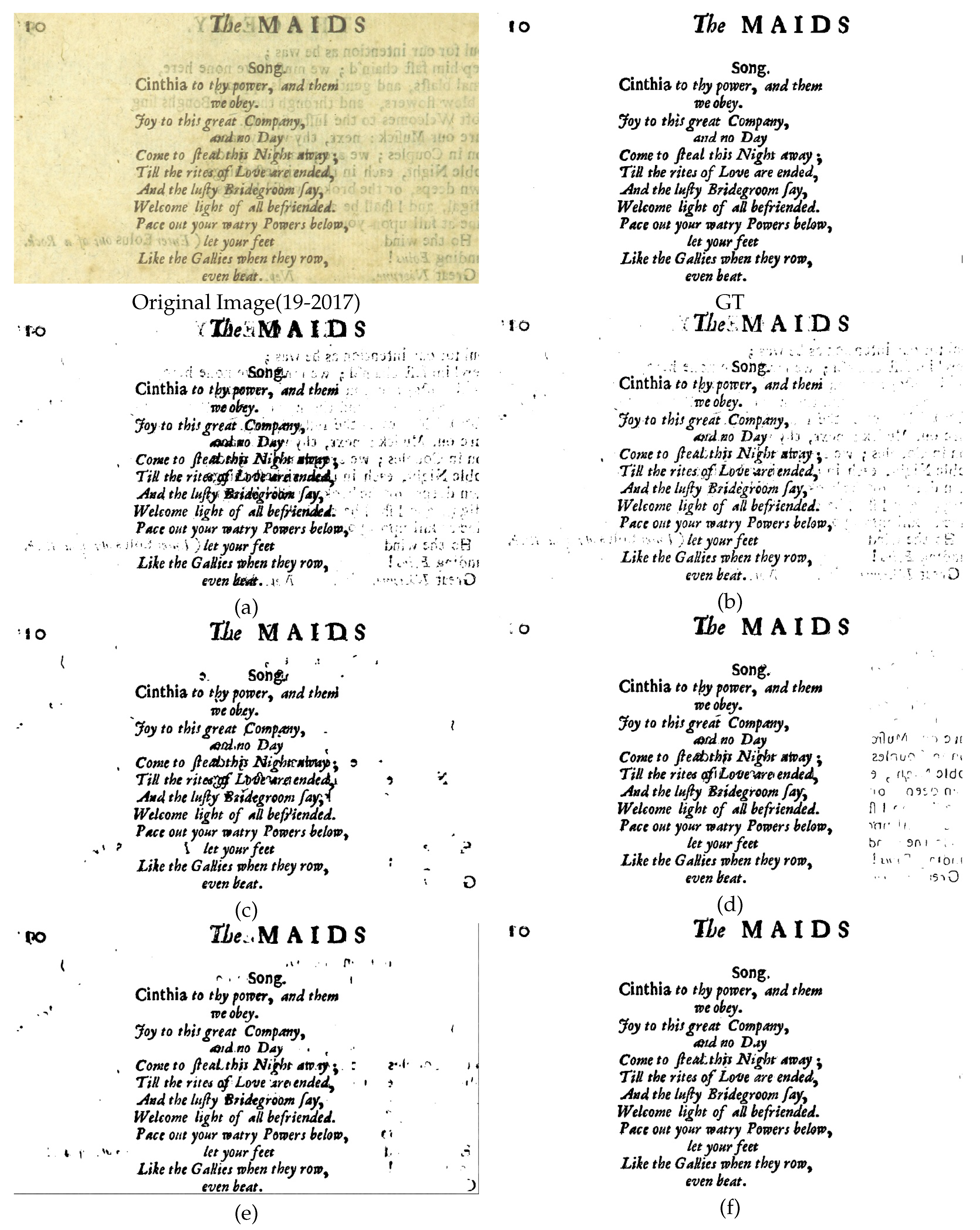
Only the proposed method obtains fully satisfactory results for binarization of document images in Figure 9. From the binarization results of the traditional methods (Otsu [20], Sauvola [22] and Xiong et al. [46]) in Figure 9, we can see that, For shadows with similar text information in the background, it is difficult for these methods to correctly segment them into background content. For the binarization results of Rezanezhad et al. [63], compared with Calvo and Gallego [19], the background content near the text can be segmented well, but the photocopy contaminated area far away from the text area cannot be correctly segmented. This is because the model of Rezanezhad et al [63] has limited feature learning ability for the global information of document images. The advantage of the proposed model is that it can use the lightweight Mobile ViT block module to effectively fuse the global information into the local information features extracted by convolution.
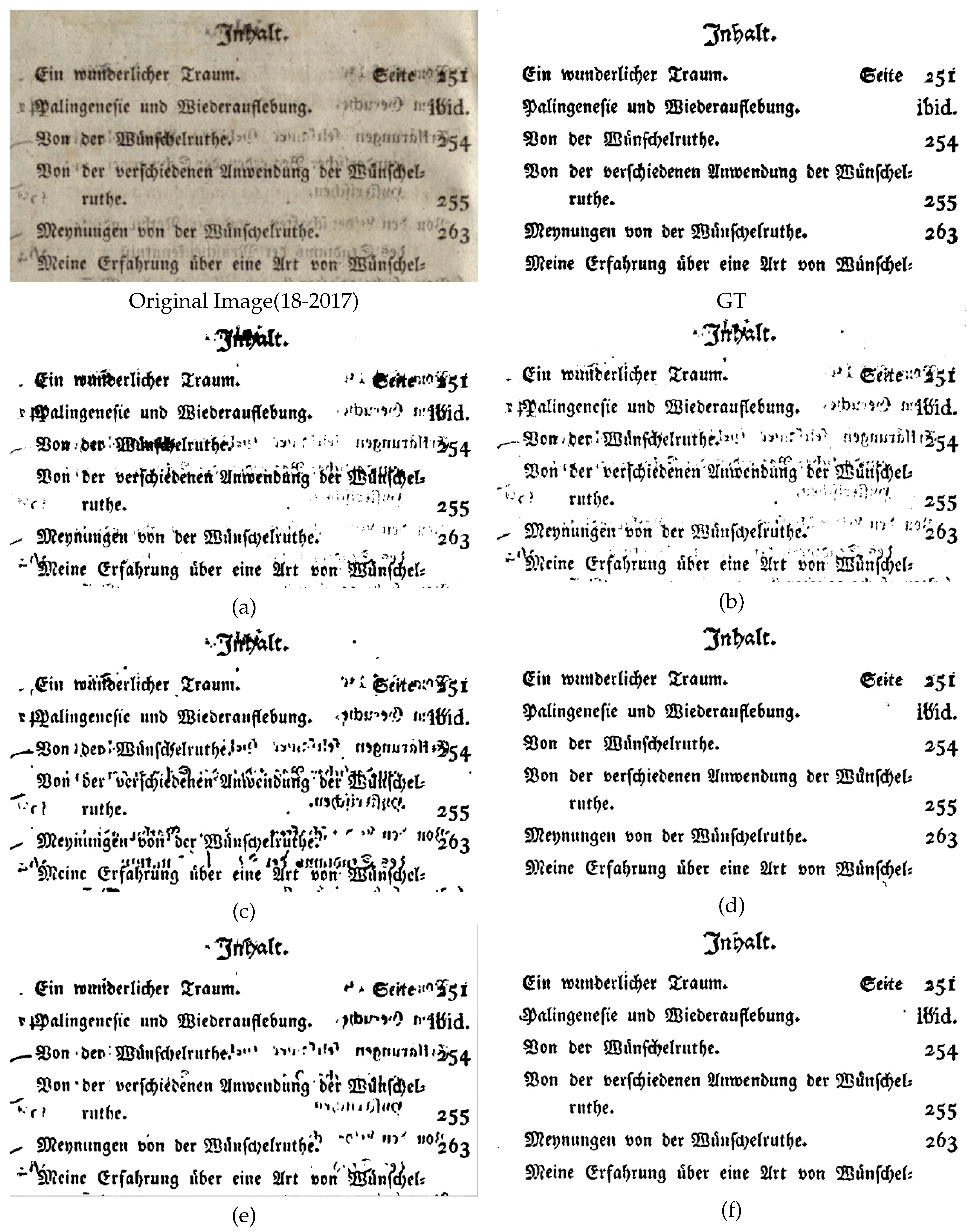
In Figure 10, the binarization results of Rezanezhad et al. [63] and the proposed model are basically satisfactory. This is because the model by Rezanezhad et al [63] uses the Transformer structure in the bottom local region of the U-Net network architecture, and the document image has a shallow background photocopy pollution compared to the document image in Figure 9. As a result, Rezanezhad et al. [63] do a good job of separating background from text content.
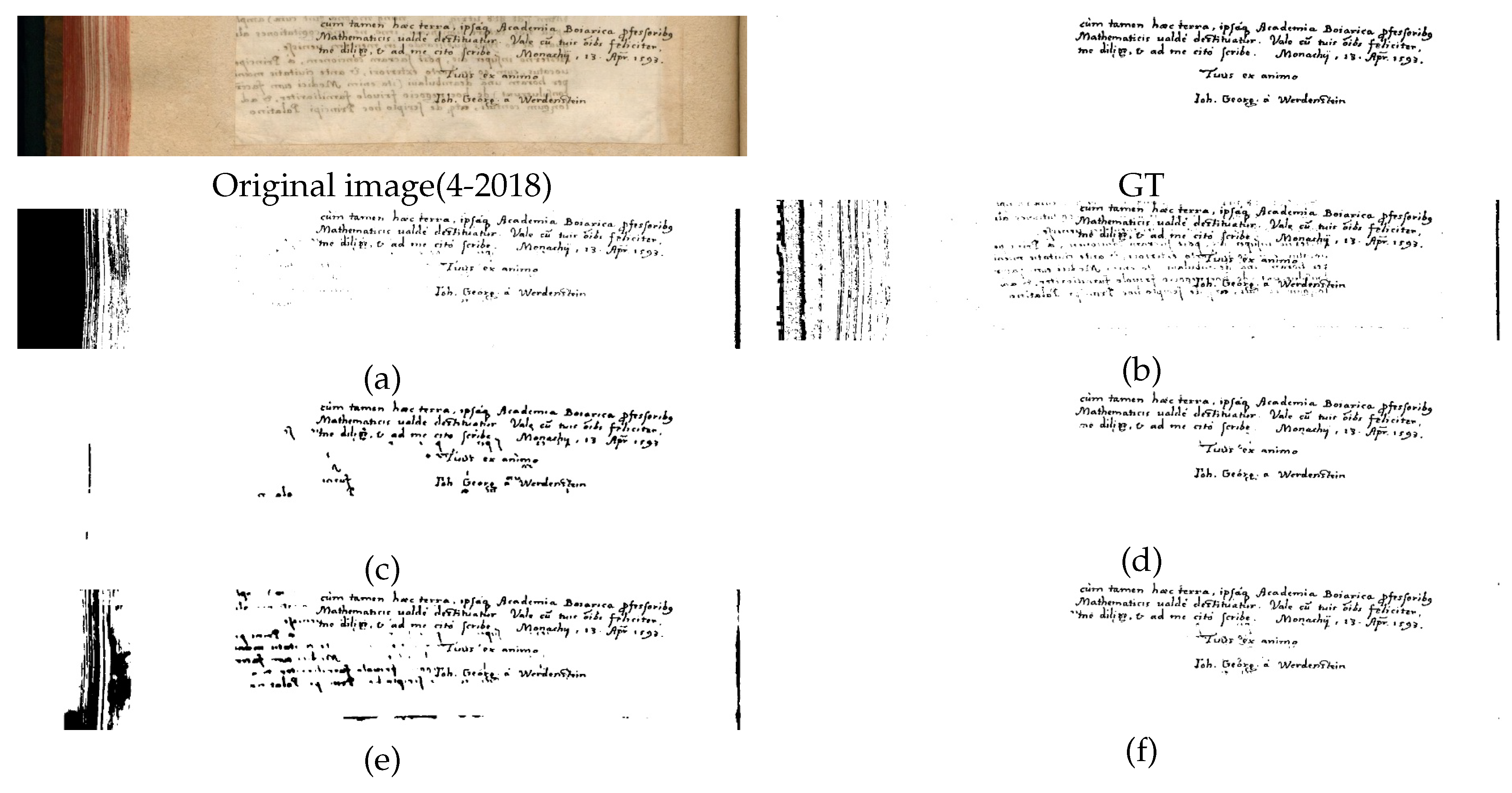
Similar to the binarization results in Figure 10. In Figure 11, the binarization results of Rezanezhad et al. [63] and the proposed model are both relatively satisfactory. Figure 11 shows that the binarization of Otsu [20] is significantly better than that of Sauvola [22] because the photocopied text content in the background is lighter in color than the text content in the foreground. As a result, the Transformer used by Rezanezhad et al. [63] does a good job of separating background content from real text content in small regions of the model. In addition, for the model training process of DIBCO2018 [16] dataset, 10 more effective datasets (6.2%) are used than that of DIBCO2017 [15], which plays an important role in improving the performance of the model.
For the binarization results of all methods in Figure 12, visually, there is a big difference between the binarization results of all methods and the true result (GT). The traditional three methods [20,22,46] fail to correctly preserve the shallow text content of the last two lines, and the pure convolutional method [19] also has the same problem. Rezanezhad et al. [63] show strong performance, especially in the last two lines of text display closer to the real label. This may be attributed to the large number of parameters and the integration design of multiple models. The reason may be that the model has a large number of parameters (more than four times that of the proposed model) and is based on the integration of multiple models. Specific analytical explanations will be provided in the following section on the model robustness study in quantitative experiments. Therefore, it is undeniable that the model of Rezanezhad et al. [63] does exhibit strong performance.

4.3. Quantitative Evaluation

For the quantitative numerical evaluation of the results of document image binarization processing, there are four commonly used evaluation indicators that are popular at present: Image F-measure FM, pseudo F-measure pFM [83], Peak Signal to Noise Ration (PSNR) and distance reciprocal distortion (DRD) [85]. These four evaluation metrics are used to show the quality of the obtained binarized image through different aspects, and they are significantly better than simple Accuracy.
(1) FM
Before giving the definition of FM and pFM, we first need to know the following four concepts, that is, TP, FP, TN, FN these four quantities are the correct positive value, the wrong positive value, the correct negative value, and the wrong negative value. The relationship between these four values can be clearly seen in the table below.
Table 1. Predicted Values and Ground Truth.
Predicted Values\Ground Truth Possitive (1) Negtive (0)
Possitive (1) TP FP
Negtive (0) FN TN
The usual definition of Accuracy is:
A c c u r a c y = T P + T N T P + F P + T N + F N
The F value of the image (FM), it’s defined as in equotion(8).
F M = 2 × P r e c i s i o n × R e c a l l P r e c i s i o n + R e c a l l
Where P r e c i s i o n = T P F P + T P , R e c a l l = T P F N + T P . In the binarization process, Precision is the probability that a value of 1 is correct, and Recall is the probability that a value of 1 accounts for the probability of a value of 1. We can see from the formula (7) and formula (5) that FM is more reasonable than Accuracy for the evaluation of document image binarization. Because the proportion of text in binarized text is much smaller than the pixels in the blank space, using FM metric is more scientific than simply looking at the pixel Accuracy of the whole image.
(2) pFM
The pseudo F-value (pFM) of an image, defined as:
p F M = 2 × p R e c a l l × P r e c i s i o n p R e c a l l + P r e c i s i o n
Where P r e c i s i o n is the same as defined in FM, and p R e c a l l is the percentage of the character structure in the standard image compared to the binarized image. From the above definition of FM and pFM values (59), we can clearly see that the size of these two indicators are positively correlated with the quality of the document image after binarization.
(3) PSNR
Peak signal-to-noise ratio (PSNR) is an indicator of image quality related to mean square error. It is an objective evaluation index that mainly expresses the difference between the results of image processing and the real image. In this paper, it is used to evaluate the difference between the binarization result of the document image and the binarization image of the real document image, which is calculated as follows:
P S N R = 10 × log 10 ( 2 n 1 ) 2 M S E
Where M S E is the mean squared error between the binarized image and the real binary image. For general 8bit image representation method, n = 8 , the peak value is 255 = 2 8 1 . The unit of PSNR is dB, the larger the value is, the more similar the binarization result is to the real binarized document image, which is a widely used objective index to evaluate image quality.
(4) DRD
Distance reciprocal distortion measure DRD [85] is to objectively express the distortion of visual perception of binarized document image through the distance between pixels. The specific definition is as follows:
D R D = σ k D R D K N U B M
Where D R D k is the distortion of the KTH flipped pixel and N U B N is the number of non-uniform (not all black or white pixels) blocks in the real binarized image. The larger the value of DRD, the greater the distortion of the visual perception of the binarization result. Therefore, the smaller the value of DRD, the better the binarization result of the text.
Below we have listed respectively in DIBCO2012 [11], DIBCO2017 [15] and DIBCO2018 [16]. The average values of the four indicators of the binarization results on three datasets obtained by methods [20,22,46,49,59,63,64,69,81] and our method. The results are shown in Table 2, Table 3, and Table 4.
From Table 3 and Table 3 we can clearly see that, Our simple end-to-end model outperforms other traditional methods on the mean of four common document image binarizations [20,22,46] and deep learning model with the same training dataset [49,59,63,64,69,81]. Of particular note is that the performance of our individual model also exceeds the ensemble model of Rezanezhad et al. [63], showing the absolute superiority of our model performance. However, from Table 4, Our model did not exceed the model of Jemni et al. [69] and Rezanezhad et al. [63] on the DIBCO 2018 dataset, and we also conducted experimental analysis here.
From Table 4, Our model performed worse than the model [16] on four metrics on the DIBCO2018 [16] dataset. To find out why, The four evaluation indexes of the binarization results of ten document images in the DIBCO2018 [16] dataset obtained by the model are listed in Table 5.
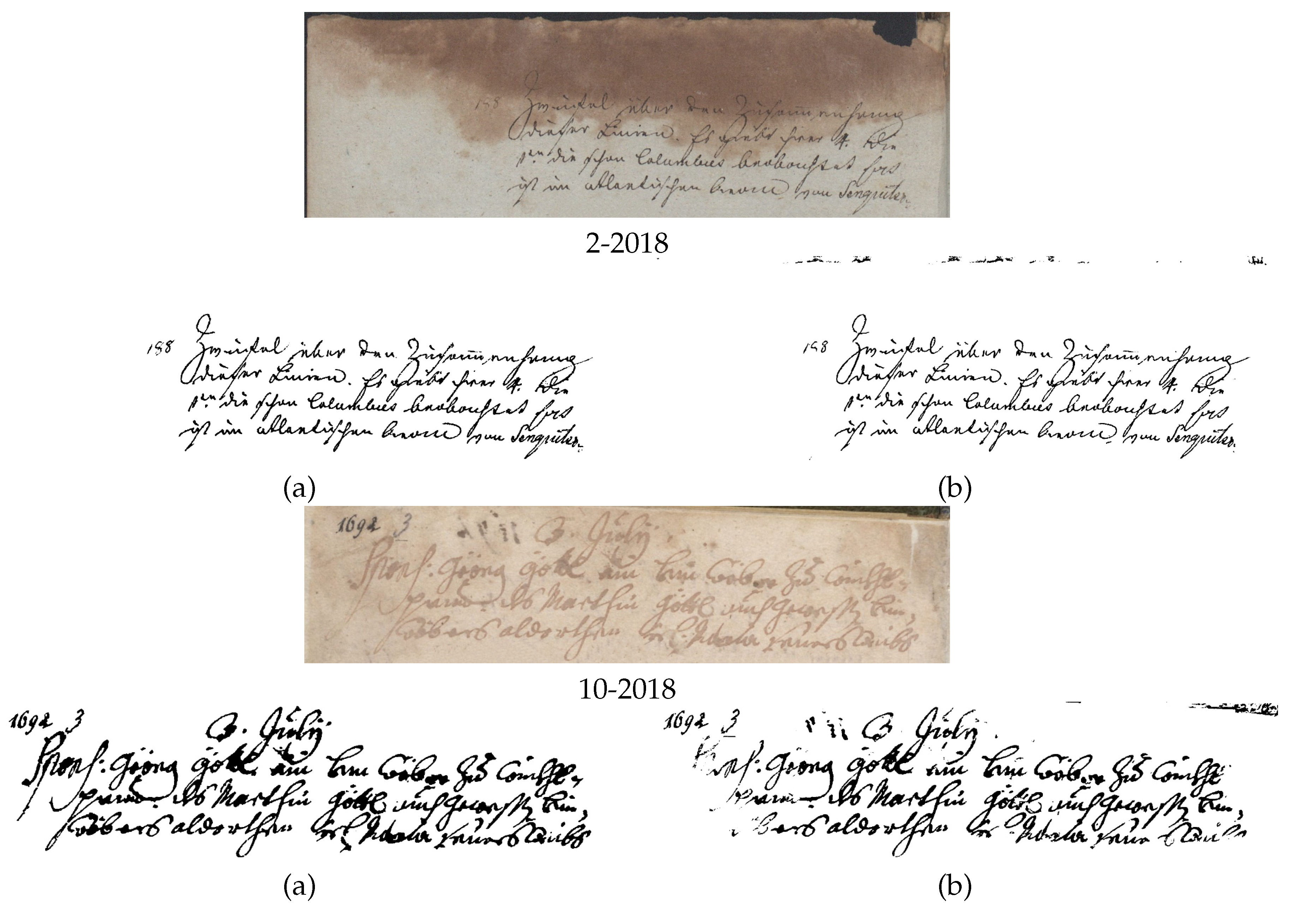
We find from the specific values in Table 5 that the binarization of images 2-2018 and 10-2018 has lower PSNR values and smaller FM values. Then we list the comparison between the binarization results of these two images obtained by our model, the original document image and GT, as shown in Figure 13.
From Figure 13(b), we can see that the difference between the binarization results of our model and the real binarization results is mainly due to the black area at the top of the image, especially the binarization results of image 2-2018 obtained by our method. The text part is almost the same as GT. It’s just that the top black area is not segmented by our model as background content. As you can see, our model is weak in learning large black areas far from the text area, which leads to the poor results of our model on the DIBCO2018 [16] dataset. The main reason for this phenomenon is that the training data set contains a smaller number of original document images with large dark areas.
Next, we will compare the robustness of the model with other methods [20,22,46,63]. The experiment is carried out on the DIBCO2019 [17] dataset with severe image damage. The specific deep learning model used is trained on the DIBCO2017 [15] dataset, because the model is obtained using the minimum number of training dataset images (162 pairs of labeled document images and their real binarization results). We also use the mean of the twenty results of the four binaryzation metrics PSNR, FM, pFM and DRD in the DIBCO2019 [17] dataset for quantitative comparison. The means for the various methods are shown in Table 6.
In Table 6, in order to more objectively and fairly measure the robustness of the model [63] and the model in this paper, Here are two examples of the [63] model. This is because the model provided by Rezanezhad et al. [63] is an ensemble of several trained models and has about 37.0M parameters, while our model has about 8.9M parameters, which are not on the same order of magnitude. In the literature [86], experiments are carried out in detail and it is verified that the corresponding changes in the network scale adjustment in depth can maintain the good performance of the original model. Therefore, we use the method proposed in [86] (the study in (d) of [86], that is, the method of reducing the number of parameters in depth) to adjust the parameter setting of the model of Rezanezhad et al. [63]. The parameter number of the proposed model is about 9.0M, which is on the same order of magnitude as that of the proposed model. At this point, the model is trained with the other training conditions being the same.
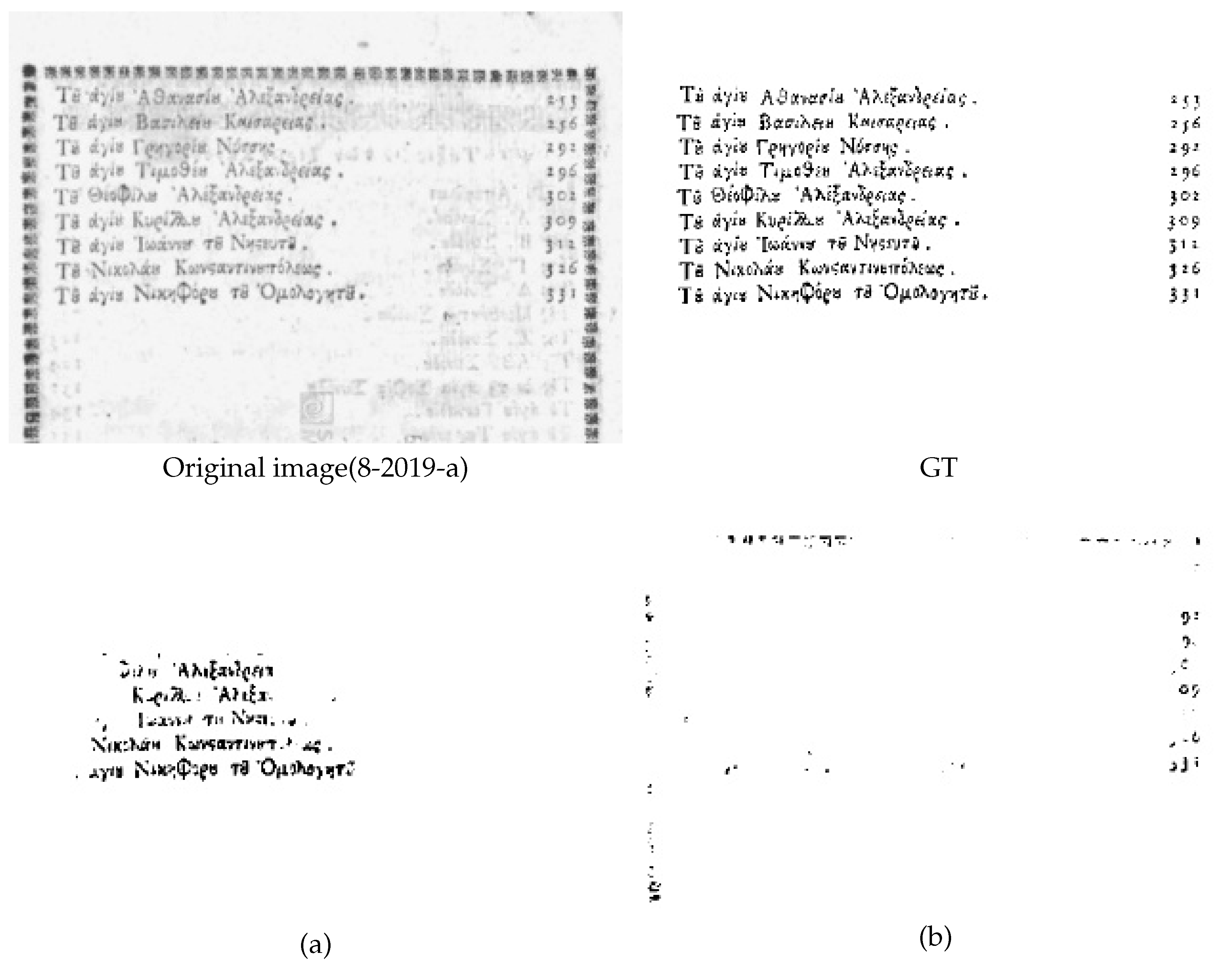
From Table 6 it is clear that the Otsu [20] method has the worst numerical performance in the binarized metrics PSNR and DRD. Although Xiong et al. [46] won the champion algorithm of the year on the DIBCO2018 [16] dataset, However, the FM and pFM numerical results on the DIBCO2019 [17] dataset are the worst, indicating that the robustness of the method is not very good. The model [63]-37.0M is optimal in Table 6 for the four indicators of image averaging in the DIBCO2019 [17] dataset. The main reason for this is that the model has a large number of parameters, which makes it the most robust. The model in this paper ranks second in the mean value of PSNR, FM and DRD for all images of the DIBCO2019 [17] dataset, and only the pFM index is inferior to the model [63]-9.0M. It can be said that the model in this paper is superior to the model of Rezanezhad et al. [63] in the same number of parameters. For the binarization results of DIBCO2019 [17] obtained by the model of this paper, we observe that there is an image (8-2019-a), the binarization obtained by the model of this paper hardly sees any real text information, and the evaluation index value is particularly low. See Figure 14.
As you can see from Figure 14, our binarization model performs poorly on images with light font colors (8-2019-a), resulting in a pFM value about 33 lower than that of [63]-9.0M. This directly leads to the lower pFM index of the proposed model on the DIBCO2019 [17] dataset.

5. Ablation experiment

In this subsection, we analyze the effect of the core module role in the model and its corresponding channel Settings on the network performance. All ablation experiments are validated on the DIBCO2017 [15] dataset.

5.1. Experiments on the Performance of Mobile ViT Block

The first set of ablation experiments is an exploration of the number of components of the proposed model Mobile ViT block. The specific experiment is completed by changing the number of this module and replacing the three Mobile ViT blocks in the network with MV2 in turn under the condition that other variables are the same. We use zero, one, two and three Mobile ViT blocks to train the proposed model, and the resulting four models are denoted as M0, M1, M2, M3 (the proposed model). The four models were used to binarize the DIBCO2017 [15] dataset, and their respective average evaluation metrics (FM, pFM, PSNR, DRD) values were calculated. The results were recorded in Table 7.
In Table 7, we observe that the average value of PSNR increases gradually from M0 through M1, M2, and M3. This indicates that with the increase of the number of Mobile ViT blocks, the word similarity between the binarization results obtained by network training and the true binarization improves. From M0 to M1 to M2, and finally to M3, the values of FM and pFM experienced a process from small to large to small, and finally to the largest (DRD has a similar trend). Finally, the values of these four evaluation indicators reach the best level in M3 (the proposed model). Therefore, our choice of three Mobile ViT blocks is reasonable.

5.2. Experiments on the Number of Channels in Mobile ViT Block

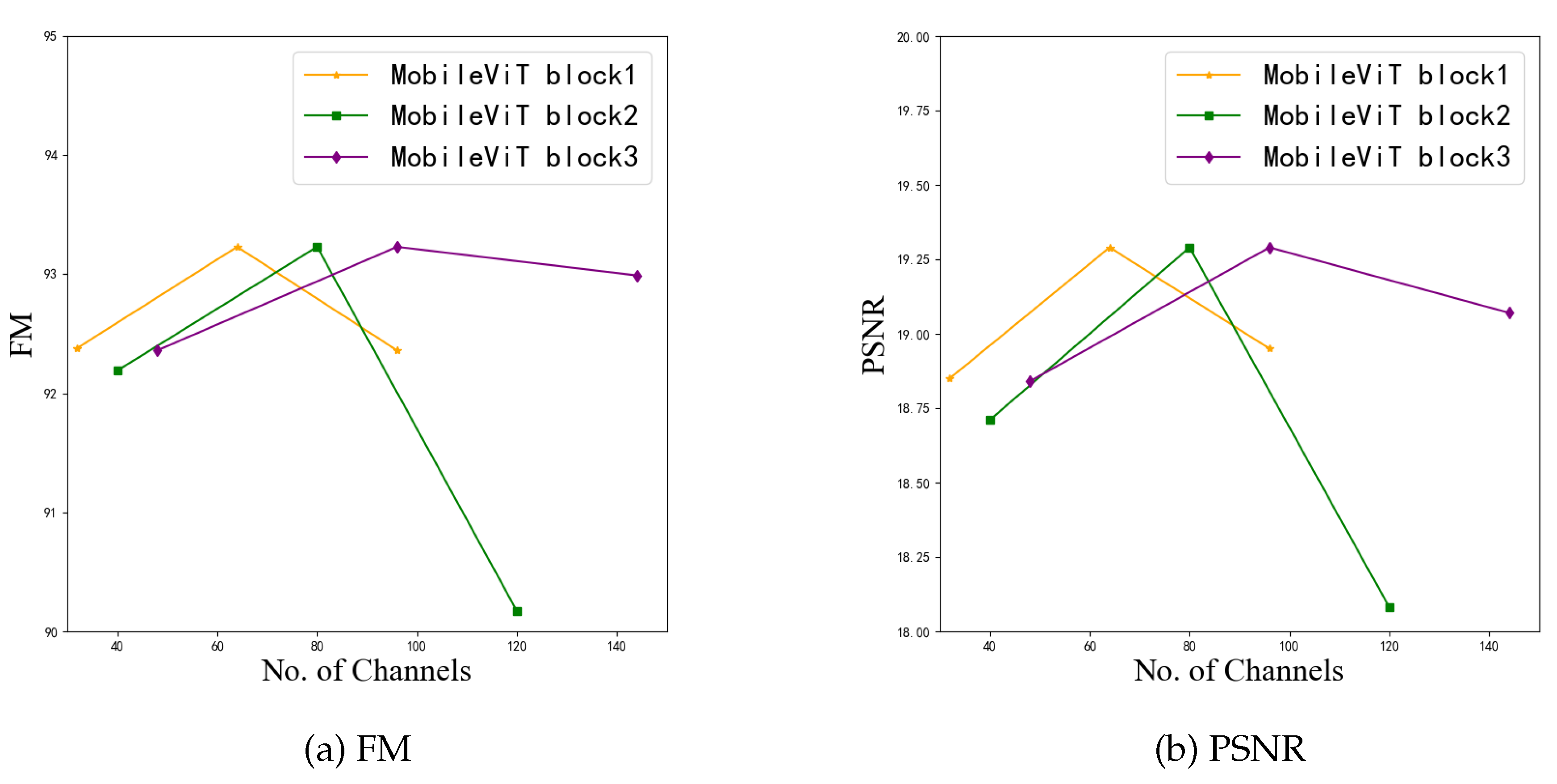
The second ablation experiment is to analyze the effect of the number of channels in the three Mobile ViT blocks on the performance of the model. The specific operation is that the number of channels of 32, 64 and 96 are used for the first Mobile ViT block, the number of channels of 40, 80 and 96 are used for the second, and the number of channels of 48, 96 and 144 are used for the third to train the model. The number of channels used in this paper is 64, 80 and 96 in turn. In the experiment, the number of channels in the first two modules is controlled, and different numbers of channels are used in the third module. The average FM and PSNR of the final binarization results with different numbers of channels are shown in the respective line charts in Figure 15.
From Figure 15, we can see that for both FM index value and PSNR value, when the number of three channels is selected as the intermediate value, the two evaluation indexes achieve the best level in each Mobile ViT block. Therefore, the number of intermediate channels selected by the proposed model is reasonable.

6. Conclusions

The work of this paper mainly implements the model of document image binarization by introducing the Mobile ViT block module into the architecture of U-Net. The proposed model is a simple end-to-end model with 76% fewer parameters compared to the similar Rezanezhad et al. [63] model. On the two datasets of DIBCO2012 and DIBCO2017 [11,15], the proposed model shows better performance, and significantly improves common evaluation indicators such as FM, pFM, PSNR and DRD. To verify the robustness of the model, we performed document image binarization processing on the DIBCO2019 [17] dataset by comparing the models of Rezanezhad et al [63] with two parameter quantities and the classic traditional method with our model. By comparing the mean values of the four evaluation indexes of the binarization results obtained by different methods, it is confirmed that the proposed model has good robustness. Finally, in order to analyze the role of the core module in the proposed model and the influence of its corresponding channel Settings on the network performance, we conduct two sets of ablation experiments, verified the rationality of the proposed model through the comparative analysis of experimental results.

Author Contributions

Conceptualization, L.Z. and Y.W.; methodology, L.Z. and K.W.; software, L.Z. and K.W.; validation, L.Z.; formal analysis, L.Z.; investigation, L.Z.; resources, L.Z.; data curation, L.Z.; writing—original draft preparation, L.Z.; writing—review and editing, L.Z. and K.W.; visualization, L.Z.; supervision, Y.W.; project administration, Y.W.; funding acquisition, Y.W. All authors have read and agreed to the published version of the manuscript.

Funding

This research received no external funding.

Conflicts of Interest

The authors declare no conflict of interest.

References

  1. Pan, Y.F.; Hou, X.; Liu, C.L. Text Localization in Natural Scene Images Based on Conditional Random Field. 2009 10th International Conference on Document Analysis and Recognition, 2009, pp. 6–10. [CrossRef]
  2. Gupta, M.R.; Jacobson, N.P.; Garcia, E.K. OCR binarization and image pre-processing for searching historical documents. Pattern Recognition 2007, 40, 389–397. [Google Scholar] [CrossRef]
  3. Saabni, R.; Asi, A.; El-Sana, J. Text line extraction for historical document images. Pattern Recognit. Lett. 2014, 35, 23–33. [Google Scholar] [CrossRef]
  4. He, S.; Wiering, M.; Schomaker, L. Junction detection in handwritten documents and its application to writer identification. Pattern Recognit. 2015, 48, 4036–4048. [Google Scholar] [CrossRef]
  5. Giotis, A.P.; Sfikas, G.; Gatos, B.; Nikou, C. A survey of document image word spotting techniques. Pattern Recognit. 2017, 68, 310–332. [Google Scholar] [CrossRef]
  6. Kumar, G.; Bhatia, P.K. A Detailed Review of Feature Extraction in Image Processing Systems. 2014 Fourth International Conference on Advanced Computing & Communication Technologies, 2014, pp. 5–12. [CrossRef]
  7. Smith, R.W. An Overview of the Tesseract OCR Engine. Ninth International Conference on Document Analysis and Recognition (ICDAR 2007) 2007, 2, 629–633. [Google Scholar] [CrossRef]
  8. Gatos, B.; Ntirogiannis, K.; Pratikakis, I. ICDAR 2009 Document Image Binarization Contest (DIBCO 2009). 2009 10th International Conference on Document Analysis and Recognition, 2009, pp. 1375–1382. [CrossRef]
  9. Pratikakis, I.; Gatos, B.; Ntirogiannis, K. H-DIBCO 2010 - Handwritten Document Image Binarization Competition. 2010 12th International Conference on Frontiers in Handwriting Recognition, 2010, pp. 727–732. [CrossRef]
  10. Pratikakis, I.; Gatos, B.; Ntirogiannis, K. ICDAR 2011 Document Image Binarization Contest (DIBCO 2011). 2011 International Conference on Document Analysis and Recognition, 2011, pp. 1506–1510. [CrossRef]
  11. Pratikakis, I.; Gatos, B.; Ntirogiannis, K. ICFHR 2012 Competition on Handwritten Document Image Binarization (H-DIBCO 2012). 2012 International Conference on Frontiers in Handwriting Recognition, 2012, pp. 817–822. [CrossRef]
  12. Pratikakis, I.; Gatos, B.; Ntirogiannis, K. ICDAR 2013 Document Image Binarization Contest (DIBCO 2013). 2013 12th International Conference on Document Analysis and Recognition, 2013, pp. 1471–1476. [CrossRef]
  13. Ntirogiannis, K.; Gatos, B.; Pratikakis, I. ICFHR2014 Competition on Handwritten Document Image Binarization (H-DIBCO 2014). 2014 14th International Conference on Frontiers in Handwriting Recognition, 2014, pp. 809–813. [CrossRef]
  14. Pratikakis, I.; Zagoris, K.; Barlas, G.; Gatos, B. ICFHR2016 Handwritten Document Image Binarization Contest (H-DIBCO 2016). 2016 15th International Conference on Frontiers in Handwriting Recognition (ICFHR), 2016, pp. 619–623. [CrossRef]
  15. Pratikakis, I.; Zagoris, K.; Barlas, G.; Gatos, B. ICDAR2017 Competition on Document Image Binarization (DIBCO 2017). 2017 14th IAPR International Conference on Document Analysis and Recognition (ICDAR), 2017, Vol. 01, pp. 1395–1403. [CrossRef]
  16. Pratikakis, I.; Zagori, K.; Kaddas, P.; Gatos, B. ICFHR 2018 Competition on Handwritten Document Image Binarization (H-DIBCO 2018). 2018 16th International Conference on Frontiers in Handwriting Recognition (ICFHR), 2018, pp. 489–493. [CrossRef]
  17. Pratikakis, I.; Zagoris, K.; Karagiannis, X.; Tsochatzidis, L.; Mondal, T.; Marthot-Santaniello, I. ICDAR 2019 Competition on Document Image Binarization (DIBCO 2019). 2019 International Conference on Document Analysis and Recognition (ICDAR), 2019, pp. 1547–1556. [CrossRef]
  18. Seuret, M.; Nicolaou, A.; Stutzmann, D.; Maier, A.; Christlein, V. ICFHR 2020 Competition on Image Retrieval for Historical Handwritten Fragments. 2020 17th International Conference on Frontiers in Handwriting Recognition (ICFHR), 2020, pp. 216–221. [CrossRef]
  19. Calvo-Zaragoza, J.; Gallego, A.J. A selectional auto-encoder approach for document image binarization. Pattern Recognition 2019, 86, 37–47. [Google Scholar] [CrossRef]
  20. Otsu, N. A Threshold Selection Method from Gray-Level Histograms. IEEE Transactions on Systems, Man, and Cybernetics 1979, 9, 62–66. [Google Scholar] [CrossRef]
  21. Niblack, W. An introduction to digital image processing, 1986.
  22. Sauvola, J.; Pietikäinen, M. Adaptive document image binarization. Pattern Recognition 2000, 33, 225–236. [Google Scholar] [CrossRef]
  23. Wolf, C.; Jolion, J.M. Extraction and recognition of artificial text in multimedia documents. Formal Pattern Analysis & Applications 2004, 6, 309–326. [Google Scholar]
  24. Bernsen, J. Dynamic thresholding of grey-level images. ICPR`86: Proceedings of International Conference on Pattern Recognition, 1986, pp. 1251–1255.
  25. Gatos, B.; Pratikakis, I.; Perantonis, S. Adaptive degraded document image binarization. Pattern Recognition 2006, 39, 317–327. [Google Scholar] [CrossRef]
  26. Khurshid, K.; Siddiqi, I.; Faure, C.; Vincent, N. Comparison of Niblack inspired binarization methods for ancient documents. Electronic imaging, 2009.
  27. Jiang, L.; Chen, K.; Yan, S.; Zhou, Y.; Guan, H. Adaptive Binarization for Degraded Document Images. 2009 International Conference on Information Engineering and Computer Science, 2009, pp. 1–4. [CrossRef]
  28. Bataineh, B.; Abdullah, S.N.H.S.; Omar, K. An adaptive local binarization method for document images based on a novel thresholding method and dynamic windows. Pattern Recognition Letters 2011, 32, 1805–1813. [Google Scholar] [CrossRef]
  29. Su, B.; Lu, S.; Tan, C.L. Robust Document Image Binarization Technique for Degraded Document Images. IEEE Transactions on Image Processing 2013, 22, 1408–1417. [Google Scholar] [CrossRef] [PubMed]
  30. Hadjadj, Z.; Meziane, A.; Cherfa, Y.; Cheriet, M.; Setitra, I. ISauvola: Improved Sauvola’s Algorithm for Document Image Binarization. Image Analysis and Recognition, 2016, Vol. 9730, pp. 737–745. [CrossRef]
  31. Mustafa, W.A.; Kader, M.M.M.A. Binarization of Document Image Using Optimum Threshold Modification. Journal of Physics: Conference Series 2018, 1019. [Google Scholar] [CrossRef]
  32. Zemouri, E.T.; Chibani, Y.; Brik, Y. Enhancement of Historical Document Images by Combining Global and Local Binarization Technique. International Journal of Information Engineering and Electronic Business 2014, 4. [Google Scholar] [CrossRef]
  33. Ntirogiannis, K.; Gatos, B.; Pratikakis, I. A combined approach for the binarization of handwritten document images. Pattern Recognit. Lett. 2014, 35, 3–15, Frontiersin Handwriting Processing. [Google Scholar] [CrossRef]
  34. Chaudhary, P.; Ambedkar, B. AN EFFECTIVE AND ROBUST TECHNIQUE FOR THE BINARIZATION OF DEGRADED DOCUMENT IMAGES. Int. J. Res. Eng. Technol. 2014, 03, 140–145. [Google Scholar]
  35. Saddami, K.; Arnia, F.; Away, Y.; Munadi, K. Kombinasi Metode Nilai Ambang Lokal dan Global untuk Restorasi Dokumen Jawi Kuno. J. Teknol. Inf. Dan Ilmu Komput. 2020, 7, 163–170. [Google Scholar] [CrossRef]
  36. Lu, S.; Su, B.; Tan, C. Document image binarization using background estimation and stroke edges. Int. J. Doc. Anal. Recognit. (IJDAR) 2010, 13, 303–314. [Google Scholar] [CrossRef]
  37. Santhanaprabhu, G.; Karthick, B.; Srinivasan, P.; Vignesh, R.; Sureka, K. Extraction and Document Image Binarization Using Sobel Edge Detection. J. Eng. Res. Appl. 2014, 4, 15–21. [Google Scholar]
  38. Lelore, T.; Bouchara, F. FAIR: A Fast Algorithm for Document Image Restoration. IEEE Trans. Pattern Anal. Mach. Intell. 2013, 35, 2039–2048. [Google Scholar] [CrossRef]
  39. Holambe, S.; Shinde, U.; Choudhari, B. Image Binarization for Degraded Document Images. Int. J. Comput. Appl. 2015, 128, 38–43. [Google Scholar]
  40. Jia, F.; Shi, C.; He, K.; Wang, C.; Xiao, B. Document image binarization using structural symmetry of strokes. 2016 15th International Conference on Frontiers in Handwriting Recognition (ICFHR). IEEE, 2016, pp. 411–416.
  41. Lai, A.N.; Lee, G. Binarization by local k-means clustering for Korean text extraction. 2008 IEEE International Symposium on Signal Processing and Information Technology. IEEE, 2008, pp. 117–122.
  42. Tong, L.J.; Chen, K.; Zhang, Y.; Fu, X.L.; Duan, J.Y. Document image binarization based on NFCM. 2009 2nd International Congress on Image and Signal Processing. IEEE, 2009, pp. 1–5.
  43. Biswas, B.; Bhattacharya, U.; Chaudhuri, B.B. A global-to-local approach to binarization of degraded document images. 2014 22nd International Conference on Pattern Recognition. IEEE, 2014, pp. 3008–3013.
  44. Soua, M.; Kachouri, R.; Akil, M. GPU parallel implementation of the new hybrid binarization based on Kmeans method (HBK). J. Real-Time Image Process 2018, 14, 363–377. [Google Scholar] [CrossRef]
  45. Annabestani, M.; Saadatmand-Tarzjan, M. A new threshold selection method based on fuzzy expert systems for separating text from the background of document images. Iran. J. Sci. Technol. Trans. Electr. Eng. 2019, 43, 219–231. [Google Scholar] [CrossRef]
  46. Xiong, W.; Zhou, L.; Yue, L.; Li, L.; Wang, S. An enhanced binarization framework for degraded historical document images. EURASIP Journal on Image and Video Processing 2021, 2021, 13. [Google Scholar] [CrossRef]
  47. Pastor-Pellicer, J.; España-Boquera, S.; Zamora-Martínez, F.; Afzal, M.Z.; Castro-Bleda, M.J. Insights on the Use of Convolutional Neural Networks for Document Image Binarization. Advances in Computational Intelligence; Rojas, I., Joya, G., Catala, A., Eds.; Springer International Publishing: Cham, 2015; pp. 115–126. [Google Scholar]
  48. Long, J.; Shelhamer, E.; Darrell, T. Fully convolutional networks for semantic segmentation. Proceedings of the IEEE conference on computer vision and pattern recognition, 2015, pp. 3431–3440.
  49. Tensmeyer, C.; Martinez, T. Document image binarization with fully convolutional neural networks. 2017 14th IAPR international conference on document analysis and recognition (ICDAR). IEEE, 2017, Vol. 1, pp. 99–104.
  50. Calvo-Zaragoza, J.; Vigliensoni, G.; Fujinaga, I. Pixel-wise binarization of musical documents with convolutional neural networks. 2017 Fifteenth IAPR International Conference on Machine Vision Applications (MVA), 2017, pp. 362–365. [CrossRef]
  51. Vo, Q.N.; Kim, S.H.; Yang, H.J.; Lee, G. Binarization of degraded document images based on hierarchical deep supervised network. Pattern Recognit. 2018, 74, 568–586. [Google Scholar] [CrossRef]
  52. Ma, K.; Shu, Z.; Bai, X.; Wang, J.; Samaras, D. Docunet: Document image unwarping via a stacked u-net. Proceedings of the IEEE conference on computer vision and pattern recognition, 2018, pp. 4700–4709.
  53. He, S.; Schomaker, L. DeepOtsu: Document enhancement and binarization using iterative deep learning. Pattern Recognit. 2019, 91, 379–390. [Google Scholar] [CrossRef]
  54. Bezmaternykh, P.; Ilin, D.; Nikolaev, D. U-Net-bin: hacking the document image binarization contest. Comput. Opt. 2019, 43, 825–832. [Google Scholar] [CrossRef]
  55. Ayyalasomayajula, K.R.; Malmberg, F.; Brun, A. PDNet: Semantic segmentation integrated with a primal-dual network for document binarization. Pattern Recognit. Lett. 2019, 121, 52–60. [Google Scholar] [CrossRef]
  56. Huang, X.; Li, L.; Liu, R.; Xu, C.; Ye, M. Binarization of degraded document images with global-local U-Nets. Optik 2020, 203, 164025. [Google Scholar] [CrossRef]
  57. Xiong, W.; Jia, X.; Yang, D.; Ai, M.; Li, L.; Wang, S. DP-LinkNet: A convolutional network for historical document image binarization. KSII Transactions on Internet and Information Systems (TIIS) 2021, 15, 1778–1797. [Google Scholar]
  58. Xiong, W.; Yue, L.; Zhou, L.; Wei, L.; Li, M. FD-Net: A Fully Dilated Convolutional Network for Historical Document Image Binarization. Pattern Recognition and Computer Vision: 4th Chinese Conference, PRCV 2021, Beijing, China, October 29–November 1, 2021, Proceedings, Part I 4. Springer, 2021, pp. 518–529.
  59. Kang, S.; Iwana, B.K.; Uchida, S. Complex image processing with less data—Document image binarization by integrating multiple pre-trained U-Net modules. Pattern Recognition 2021, 109, 107577. [Google Scholar] [CrossRef]
  60. Dey, A.; Das, N.; Nasipuri, M. Variational Augmentation for Enhancing Historical Document Image Binarization. arXiv preprint arXiv:2211.06581, arXiv:2211.06581 2022.
  61. Yang, Z.; Xiong, Y.; Wu, G. GDB: Gated convolutions-based Document Binarization. arXiv preprint arXiv:2302.02073, arXiv:2302.02073 2023.
  62. Zhao, P.; Wang, W.; Zhang, G.; Lu, Y. Alleviating pseudo-touching in attention U-Net-based binarization approach for the historical Tibetan document images. Neural Comput. Appl. 2023, 35, 13791–13802. [Google Scholar] [CrossRef]
  63. Vahid, R.; Konstantin, B.; Clemens, N. A hybrid cnn-transformer model for historical document image binarization. HIP ’23: 7th International Workshop on Historical Document Imaging and Processing, San Jose CA USA, 2023, pp. 79–84.
  64. Zhao, J.; Shi, C.; Jia, F.; Wang, Y.; Xiao, B. Document image binarization with cascaded generators of conditional generative adversarial networks. Pattern Recognit. 2019, 96, 106968. [Google Scholar] [CrossRef]
  65. De, R.; Chakraborty, A.; Sarkar, R. Document Image Binarization Using Dual Discriminator Generative Adversarial Networks. IEEE Signal Processing Letters 2020, PP, 1–1. [Google Scholar] [CrossRef]
  66. Souibgui, M.A.; Kessentini, Y. DE-GAN: A Conditional Generative Adversarial Network for Document Enhancement. IEEE Trans. Pattern Anal. Mach. Intell. 2022, 44, 1180–1191. [Google Scholar] [CrossRef] [PubMed]
  67. Kumar, A.; Ghose, S.; Chowdhury, P.N.; Roy, P.P.; Pal, U. UDBNET: Unsupervised Document Binarization Network via Adversarial Game. 2020 25th International Conference on Pattern Recognition (ICPR). IEEE, 2021, pp. 7817–7824.
  68. Suh, S.; Kim, J.; Lukowicz, P.; Lee, Y.O. Two-stage generative adversarial networks for binarization of color document images. Pattern Recognition, 2022; 108810. [Google Scholar]
  69. Jemni, S.K.; Souibgui, M.A.; Kessentini, Y.; Fornés, A. Enhance to read better: A multi-task adversarial network for handwritten document image enhancement. Pattern Recognition 2022, 123, 108370. [Google Scholar] [CrossRef]
  70. Racjesh, B.; Agrawal, M.K.; Bhuva, M.; Kishore, K.; Javed, M. Document Image Binarization in JPEG Compressed Domain using Dual Discriminator Generative Adversarial Networks. In Computer Vision and Machine Intelligence: Proceedings of CVMI 2022; Springer, 2023; pp. 761–774.
  71. Fathallah, A.; El Yacoubi, M.; Amara, N.B. EHDI: enhancement of historical document images via generative adversarial network. 18th International Conference on Computer Vision Theory and Applications (VISAPP). SCITEPRESS-Science and Technology Publications, 2023, Vol. 4, pp. 238–245.
  72. Guo, Y.; Ji, C.; Zheng, X.; Wang, Q.; Luo, X. Multi-scale multi-attention network for moiré document image binarization. Signal Process. Image Commun. 2021, 90, 116046. [Google Scholar] [CrossRef]
  73. Pandey, S.; Bharti, J. Document Enhancement and Binarization Using Deep Learning Approach. Proceedings of Third International Conference on Intelligent Computing, Information and Control Systems: ICICCS 2021. Springer, 2022, pp. 133–145.
  74. Peng, X.; Wang, C.; Cao, H. Document binarization via multi-resolutional attention model with DRD loss. 2019 International Conference on Document Analysis and Recognition (ICDAR). IEEE, 2019, pp. 45–50.
  75. Goodfellow, I.; Pouget-Abadie, J.; Mirza, M.; Xu, B.; Warde-Farley, D.; Ozair, S.; Courville, A.; Bengio, Y. Generative Adversarial Networks. ML 2014, [1406.2661].
  76. Ronneberger, O.; Fischer, P.; Brox, T. U-Net: Convolutional Networks for Biomedical Image Segmentation. Medical Image Computing and Computer-Assisted Intervention – MICCAI 2015; Navab, N., Hornegger, J., Wells, W.M., Frangi, A.F., Eds.; Springer International Publishing: Cham, 2015; pp. 234–241. [Google Scholar]
  77. Nikitin, F.; Dokholyan, V.; Zharikov, I.; Strijov, V. U-Net Based Architectures for Document Text Detection and Binarization, 2019. [CrossRef]
  78. Detsikas, N.; Mitianoudis, N.; Papamarkos, N. A Dilated MultiRes Visual Attention U-Net for historical document image binarization. Signal Processing: Image Communication 2024, 122, 117102. [Google Scholar] [CrossRef]
  79. Dumoulin, V.; Visin, F. A guide to convolution arithmetic for deep learning, 2018. arXiv:stat.ML/1603.07285].
  80. Ioffe, S.; Szegedy, C. Batch normalization: Accelerating deep network training by reducing internal covariate shift. International conference on machine learning. pmlr, 2015, pp. 448–456.
  81. Souibgui, M.A.; Biswas, S.; Jemni, S.K.; Kessentini, Y.; Fornés, A.; Lladós, J.; Pal, U. Docentr: An end-to-end document image enhancement transformer. 2022 26th International Conference on Pattern Recognition (ICPR). IEEE, 2022, pp. 1699–1705.
  82. Burie, J.C.; Coustaty, M.; Hadi, S.; Kesiman, M.W.A.; Ogier, J.M.; Paulus, E.; Sok, K.; Sunarya, I.M.G.; Valy, D. ICFHR2016 Competition on the Analysis of Handwritten Text in Images of Balinese Palm Leaf Manuscripts. 2016 15th International Conference on Frontiers in Handwriting Recognition (ICFHR), 2016, pp. 596–601. [CrossRef]
  83. Ayatollahi, S.M.; Ziaei Nafchi, H. Persian heritage image binarization competition (PHIBC 2012). 2013 First Iranian Conference on Pattern Recognition and Image Analysis (PRIA), 2013, pp. 1–4. [CrossRef]
  84. Nicolaou, A.; Christlein, V.; Riba, E.; Shi, J.; Vogeler, G.; Seuret, M. TorMentor: Deterministic dynamic-path, data augmentations with fractals. Proceedings of the IEEE/CVF Conference on Computer Vision and Pattern Recognition, 2022, pp. 2707–2711.
  85. Lu, H.; Kot, A.; Shi, Y. Distance-reciprocal distortion measure for binary document images. IEEE Signal Processing Letters 2004, 11, 228–231. [Google Scholar] [CrossRef]
  86. Tan, M.; Le, Q.V. EfficientNet: Rethinking Model Scaling for Convolutional Neural Networks. CoRR 2019, abs/1905.11946, [1905.11946]. [Google Scholar]
Figure 1. Two document images and their binarized result image. (a) Original document images from DIBCO dataset [12,16], (b) binarization results obtained by method [19].
Preprints 104573 g001
Figure 2. Some document image. Source: DIBCO dataset [14,15,17].
Preprints 104573 g002
Figure 3. Comparison of a document images with its true binarization result and the results obtained by two binarization methods. (a) original color image, (b) true binarization result (GT), (c) binarization result of Xiong et al. [46], and (d) binarization result of Rezanezhad et al. [63].
Preprints 104573 g003
Figure 4. A comparison of a document image and the results obtained by GT and two binarization methods. (a) original color image, (b) true binarization result (GT), (c) binarization result of Calvo and Gallego [19], and (d) binarization result of Rezanezhad et al. [63].
Preprints 104573 g004
Figure 5. Comparison of receptive field effects of RestNet and Transformer before and after training for the central element. The color change from light yellow to dark green indicates that the receptive field of the region has a greater influence on the central element.
Preprints 104573 g005
Figure 6. The proposed document image binary model of the overall architecture diagram. On the left side of the U-shaped structure, we introduce the MV2 and Mobile ViT block structures. The number of jump connections of the model framework is five, which can better integrate local and global features. The right annotation section of the model structure details the operation of the different colored arrows.
Preprints 104573 g006
Figure 7. Comparison of image H01-2012 and its GT and the results obtained by different binarization methods. Binarization result of (a) Otsu [20], (b)Sauvola [22], (c) Xiong et al. [46], (d) binarization results of Rezanezhad et al. [63], (e) binarization results of Calvo and Gallego [19], and (f) the proposed method.
Preprints 104573 g007
Figure 8. Comparison of image H11-2012 and its GT and the results obtained by different binarization methods. Binarization result of (a) Otsu [20], (b) Sauvola [22], (c) Xiong et al. [46], (d) binarization results of Rezanezhad et al. [63], (e) binarization results of Calvo and Gallego [19], and (f) the proposed method.
Preprints 104573 g008
Figure 9. Comparison plots of image 19-2017 and its GT and the results obtained by different binarization methods. Binarization result of (a) Otsu [20], (b) Sauvola [22], (c) Xiong et al. [46], (d) binarization results of Rezanezhad et al. [63], (e) binarization results of Calvo and Gallego [19], and (f) the proposed method.
Preprints 104573 g009
Figure 10. Comparison plots of image 18-2017 and its GT and the results obtained by different binarization methods. Binarization result of (a) Otsu [20], (b) Sauvola [22], (c) Xiong et al. [46], (d) binarization results of Rezanezhad et al. [63], (e) binarization results of Calvo and Gallego [19], and (f) the proposed method.
Preprints 104573 g010
Figure 11. Comparison plots of image 4-2018 and its GT and the results obtained by different binarization methods. Binarization result of (a) Otsu [20], (b) Sauvola [22], (c) Xiong et al. [46], (d) binarization results of Rezanezhad et al. [63], (e) binarization results of Calvo and Gallego [19], and (f) the proposed method.
Preprints 104573 g011
Figure 12. Image 5-2018 and its GT and comparison of the results obtained by different binarization methods. Binarization result of (a) Otsu [20], (b) Sauvola [22], (c) Xiong et al. [46], (d) binarization results of Rezanezhad et al. [63], (e) binarization results of Calvo and Gallego [19], and (f) the proposed method.
Preprints 104573 g012
Figure 13. Images 2-2018 and 10-2018 and their GT compared with our method. (a) GT, and (b) binarization result of our method.
Preprints 104573 g013
Figure 14. Image 8-2019-a, comparison plot of the binarized results obtained by GT and the two methods. (a) Binarization results of model [63]-9.0M (pFM=39.69), (b) binarization results of the proposed model (pFM=6.76).
Preprints 104573 g014
Figure 15. FM line plots and PSNR line plots were obtained using different number of channels in different MobileViT blocks, respectively.
Preprints 104573 g015
Table 2. Comparison of the results of different binarization methods and the proposed method on the DIBCO2012 [11] dataset. The best and second best index values are plotted in red and blue, respectively.
Algorithm PSNR FM pFM DRD
Otsu [20] 15.03 80.18 82.65 26.45
Sauvola at el. [22] 16.71 82.89 87.95 6.59
Xiong at el. [46] 21.68 94.26 95.16 2.08
Kang at el. [59] 21.37 95.16 96.44 1.13
Tensmeyer at el. [49] 20.60 92.53 96.67 2.48
Zhao at el. [64] 21.91 94.96 96.15 1.55
Jemni at el. [69] 22.00 95.18 94.63 1.62
Souibgui at el. [81] 22.29 95.31 96.29 1.60
Model 1 [63] 23.16 96.02 97.31 1.14
Model 2 [63] 23.24 96.26 97.29 1.12
Model 3 [63] 23.24 96.25 97.51 1.12
Ensenbel model [63] 23.27 96.25 97.58 1.11
Proposed method 23.32 96.37 97.73 1.08
Table 3. Comparison of the results of different binarization methods and the proposed method on the DIBCO2017 [15] dataset. The best and second best index values are plotted in red and blue, respectively.
Algorithm PSNR FM pFM DRD
Otsu [20] 13.83 77.73 77.89 15.54
Sauvola at el. [22] 14.25 77.11 84.1 8.85
Xiong at el. [46] 17.99 89.37 90.80 5.51
Kang at el. [59] 15.85 91.57 93.55 2.92
Winer Algorithm [15] 18.28 91.04 92.86 3.40
Zhao at el. [64] 17.83 90.73 92.58 3.58
Jemni at el. [69] 17.45 89.80 89.95 4.03
Souibgui at el. [81] 19.11 92.53 95.15 2.37
Model 1 [63] 18.99 92.50 95.05 2.49
Model 2 [63] 19.04 92.60 94.83 2.44
Ensenbel Model [63] 19.04 93.01 95.42 2.29
Proposed method 19.29 93.23 95.90 2.22
Table 4. Comparison of the results of different binarization methods and the proposed method on the DIBCO2018 [16] dataset. The best and second best index values are plotted in red and blue, respectively.
Algorithm PSNR FM pFM DRD
Otsu [20] 9.74 51.45 53.05 59.07
Sauvola at el. [22] 13.78 67.81 74.08 17.69
Xiong at el. [46] Winner 19.11 88.34 90.37 4.93
Kang at el. [59] 19.39 89.71 91.62 2.51
Zhao at el. [64] 18.37 87.73 90.60 4.58
Jemni at el. [69] 20.18 92.41 94.35 2.60
Souibgui at el. [81] 19.46 90.59 93.97 3.35
Model 1 [63] 19.79 90.65 93.50 3.63
Model 2 [63] 19.94 91.87 95.62 2.77
Model 3 [63] 19.88 91.46 95.00 3.00
Ensenbel Model [63] 20.29 92.47 95.99 2.50
Proposed method 19.517 90.5907 94.796 3.29
Table 5. Four evaluations of the results of the proposed method on each image of DIBCO2018 [16] dataset.
Image name PSNR FM pFM DRD
1-2018 20.23 89.96 97.52 3.18
2-2018 16.70 78.35 83.88 8.78
3-2018 18.40 95.38 99.05 1.5
4-2018 20.77 85.61 96.81 2.65
5-2018 19.02 90.17 93.96 4.25
6-2018 21.96 96.67 97.91 1.76
7-2018 22.86 93.21 94.87 2.25
8-2018 16.78 90.31 95.09 2.71
9-2018 23.39 97.01 97.44 1.23
10-2018 15.05 89.24 91.44 5.61
Average 19.52 90.59 94.80 3.39
Table 6. Comparison of the results of different binarization methods and the proposed method on the DIBCO2019 [17] dataset. The best and second best index values are plotted in red and blue, respectively.
Algorithm PSNR FM pFM DRD
Otsu [20] 9.029 47.67 48.01 109.84
Sauvola at el. [22] 13.12 64.71 66.37 21.24
Xiong at el. [46] 11.84 46.61 47.06 24.13
Model-9.0M [63] 14.99 65.81 68.10 9.98
Model-37.0M [63] 15.64 72.07 73.46 7.72
Proposed Model-8.9M 15.25 65.92 66.20 8.97
Table 7. Comparison of results on the DIBCO2017 dataset [15] using zero, one, two and three (proposed) Mobile ViT block modules.
Name PSNR FM pFM DRD
M0 18.56 91.57 94.91 2.94
M1 18.84 92.45 95.37 2.55
M2 18.88 92.39 95.12 2.75
M3 19.29 93.23 95.99 2.22
Disclaimer/Publisher’s Note: The statements, opinions and data contained in all publications are solely those of the individual author(s) and contributor(s) and not of MDPI and/or the editor(s). MDPI and/or the editor(s) disclaim responsibility for any injury to people or property resulting from any ideas, methods, instructions or products referred to in the content.
Copyright: This open access article is published under a Creative Commons CC BY 4.0 license, which permit the free download, distribution, and reuse, provided that the author and preprint are cited in any reuse.
Prerpints.org logo

Preprints.org is a free preprint server supported by MDPI in Basel, Switzerland.

Subscribe

© 2024 MDPI (Basel, Switzerland) unless otherwise stated