Fractional Boundary Element Solution for Nonlinear Nonlocal Thermoelastic Problems of Anisotropic Fibrous Polymer Nanomaterials

Preprint

Article

Fractional Boundary Element Solution for Nonlinear Nonlocal Thermoelastic Problems of Anisotropic Fibrous Polymer Nanomaterials

Altmetrics

Downloads

Views

Comments

A peer-reviewed article of this preprint also exists.

Mohamed Abdelsabour Fahmy^*,Moncef Toujani

This version is not peer-reviewed

Submitted:

24 April 2024

Posted:

28 April 2024

You are already at the latest version

Alerts

Abstract

Nonlocal theories are gaining prominence because they can solve problems which lead to unphysical conclusions in standard models. This study presents a novel fractional boundary element method (BEM) solution for nonlinear nonlocal thermoelastic problems of anisotropic fibrous polymer nanomaterials. This broad BEM solution combines two solutions: anisotropic fibrous polymer nanomaterials problem solution and nonlinear nonlocal thermoelasticity problem solution. The nonlinear nonlocal thermoelasticity problem solution divides the displacement field into complementary component and particular component. The overall displacement is generated using the boundary element technique, which is the solution to a Navier type problem, while the particular displacement is derived using local radial point. The New Modified Shift-Splitting (NMSS) approach, which reduces memory and processing time requirements, was used to solve linear systems created by BEM. Figures demonstrate the numerical findings, which show the effects of fractional and graded parameters on the thermal stresses of nonlinear nonlocal thermoelastic problems of anisotropic fibrous polymer nanomaterials. The numerical results indicate the consistency and efficiency of the proposed methodology.

Keywords:

Subject: Engineering - Mechanical Engineering

1. Introduction

Nanomaterials are materials with at least one dimension of less than 100 nanometres. Nanostructured materials are those in which the structure has been purposefully modified at the nanometer length scale to attain certain qualities [1,2]. Nanomaterials and nanostructured materials can be employed in the form of bulk materials, such as powders and ceramics. - Structured materials, which include thin films, coatings, and surfaces. - Molecular nanostructures like fullerenes, nanotubes, and other molecular assemblages [3]. These materials frequently exhibit distinctive optical, electrical, or mechanical properties. Nanomaterials are a rapidly increasing research subject that has just entered the textiles industry [4,5,6]. The precise definition of a nanoparticle is hard, but it has been proposed that a nanoparticle be defined as a particle with at least one dimension less than 100 nm. This is because a material's behavior at the nanoscale does not always match with that at the bulk size. Graphite, for example, is employed as a lubricant and is somewhat soft on the bulk scale, whereas carbon nanotubes can have a structure with extremely high tensile strength on the nanoscale [7,8]. Fahmy suggested novel boundary element solutions to thermoelastic nanostructure problems [9,10,11].

For many engineering problems, the classical theory of linear elasticity has proven to be quite effective. It is becoming increasingly evident that this theory cannot properly handle certain circumstances, including those investigated by Sudak [12,13,14,15]. According to Eringen [16], the classical elasticity is limited by the lack of an internal characteristic length scale. Nonlocal elasticity was originally studied in the framework of classical elasticity [17,18,19]. Constitutive connections for nonlocal elasticity.have been discovered by Edelen and Laws [20], Edelen et al. [21], and Eringen and Edelen [22].. Eringen and Kim [23] and Eringen et al. [24] did extensive research on linear isotropic nonlocal elastic solids, with a focus on the nonlocal constitutive relation, which includes an integral strain field term throughout the solid's volume. As a result, the stress field at a given place is impacted by the solid's total strain. Using this strategy, considerable research has been undertaken to handle fracture challenges [25,26,27,28], dislocation problems [29,30,31], focused load problems [32], and contact problems [33]. The BEM technique is very useful for calculating field derivatives like tractions and sensitivities. The integral representation formulation yields the BEM solution. This is not supported by the FEM, which only computes solutions at nodal locations.

In this study, we propose a new fractional boundary element solution for nonlinear nonlocal thermoelastic problems involving anisotropic fibrous polymer nanomaterials. This approach consists of two steps. First, address the anisotropic fibrous polymer nanoparticles problem. Second, we apply the solution of the anisotropic fibrous polymer nanomaterials problem to the nonlinear nonlocal thermoelasticity problem. The numerical findings indicate how fractional and graded parameters affect the thermal stresses of anisotropic size- and temperature-dependent fibrous polymer nanomaterials, demonstrating the validity and precision of the suggested methodology.

2. Formulation of the Problem

Let us consider a fibrous polymer nanomaterial in the

x_{1} x_{2} - p l a n e

, occupies the region

V

that bounded by

Γ

, the governing equations of fractional size- and temperature- dependent polymer problems of nonlinear nonlocal elasticity can be expressed as [10,11]

The force equilibrium equation

{\tilde{σ}}_{i j, j} + F_{i} = 0

(1)

The fractional-order temperature-dependent heat equation is

D_{τ}^{a} Θ (x, τ) = ξ \nabla [λ (Θ) \nabla Θ (x, τ)] + ξ Q (x, Θ, τ), ξ = \frac{1}{ρ (Θ) c (Θ)}

(2)

Where

{\tilde{σ}}_{i j} = {(x + 1}}^{m} (σ_{i j} + {\bar{σ}}_{i j} + {\overset{̿}{σ}}_{i j}),

(3)

{\tilde{σ}}_{i j, j} = {(x + 1)}^{m} {(σ_{i j} + {\bar{σ}}_{i j} + {\overset{̿}{σ}}_{i j})}_{, j} + \frac{m}{x + 1} {\tilde{σ}}_{j i},

(4)

σ_{i j} = σ_{(i j)} + σ_{[i j]}

(5)

σ_{(i j)} = C_{i j k l} (ε_{k k} δ_{i j} + ε_{i j} - \bar{α} Θ δ_{i j}),

(6)

σ_{[j i]} = - M_{[i, j]}, σ_{[21]} = - σ_{[12]} = - M_{[1, 2]},

(7)

{\bar{σ}}_{i j} = \bar{c} k_{B} Θ ({ε_{i j}}^{2} - 1 / ε_{i j})

(8)

{\overset{̿}{σ}}_{i j} (x) = C_{i j k l} \int_{Ω} s (x, x^{'}) ε_{k l} (x^{'}) d v (x^{'})

(9)

3. Numerical Solution

In this section, we will determine the general solution to our studied problem, which is composed of the sum of the polymer thermoelastic solution, fractional size- and temperature-dependent solution, and nonlinear nonlocal elasticity solution.

3.1. Polymer Thermoelastic Solution (PTES)

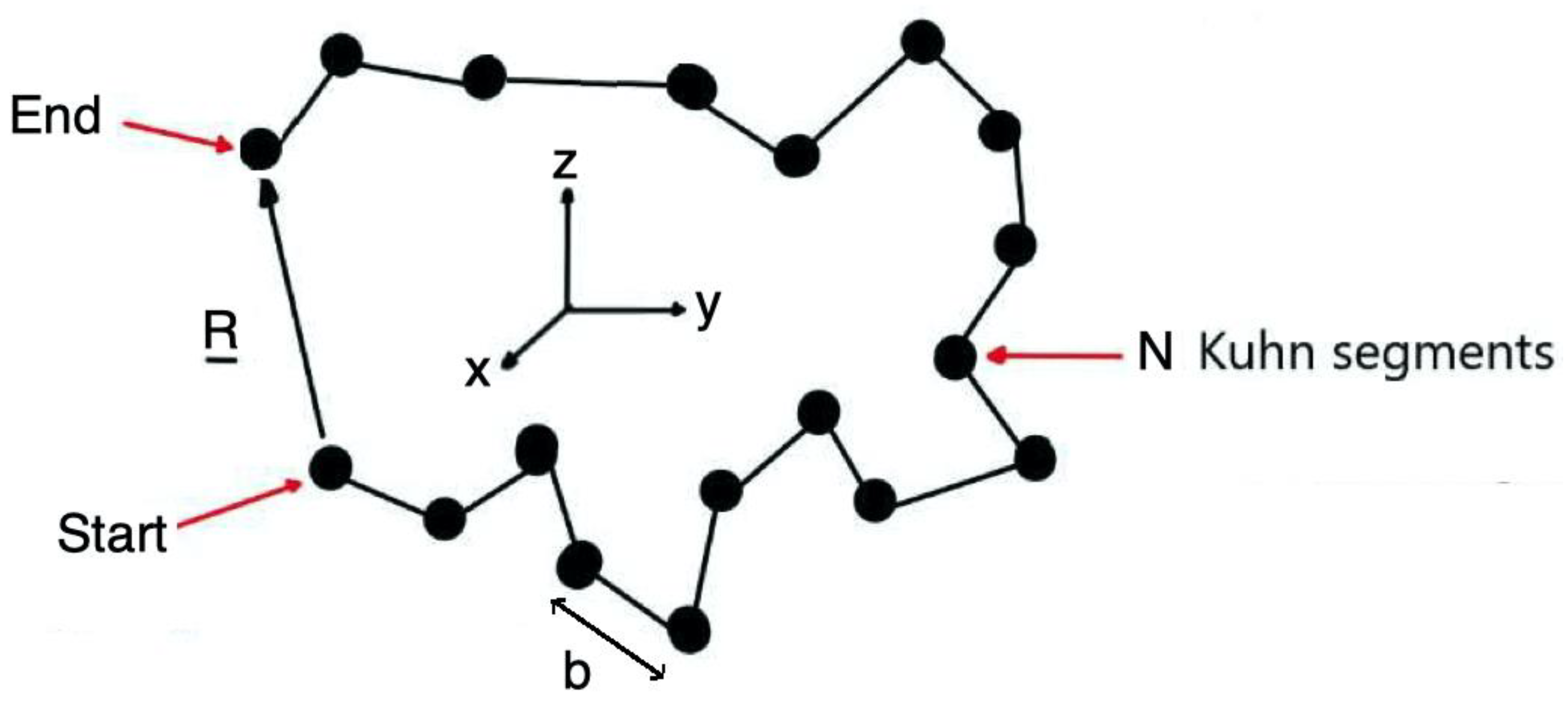
In this subsection, we analyze he mechanical deformation of fibrous polymer nanomaterial of nonlinear nonlocal thermoelasticity which shown in Figure 1 where end-to-end vector R connects the start to the end of chain.

The polymer's energy in terms of end-to-end vector is [34]

ψ (R) = (\frac{3 k_{B} θ}{2 N b^{2}}) R^{2}

(10)

which can be expressed as

f (R) = \frac{\partial ψ}{\partial R} = (\frac{3 k_{B} θ}{N b^{2}}) R

(11)

The constitutive equation for polymer elasticity [34]

{\bar{σ}}_{j i} = ρ k_{B} θ (μ - I),

(12)

μ = F F^{T}

(13)

F = [\begin{matrix} 1 & γ & 0 \\ 0 & 1 & 0 \\ 0 & 0 & 1 \end{matrix}]

(14)

{\bar{σ}}_{j i} = \bar{c} k_{B} θ [\begin{matrix} γ^{2} & γ & 0 \\ γ & 0 & 0 \\ 0 & 0 & 1 \end{matrix}] + [\begin{matrix} p & 0 & 0 \\ 0 & p & 0 \\ 0 & 0 & p \end{matrix}]

(15)

where

and

Thus from Eq. (7), we can calculate displacement which is a polymer thermoelastic solution

u^{P T E S}

from strain

ε_{i j}

3.2. Fractional Size- and Temperature- Dependent Solution (FSTDS)

The couple-stress, force-traction and couple-traction are [10]

M_{i} = \frac{1}{2} e_{i j k} M_{k j} = - 8 μ l^{2} k_{i}, l^{2} = \frac{η}{μ}

(16)

t_{i} = σ_{j i} n_{j} = C_{i j k l} (ε_{k k} δ_{i j} + ε_{i j} + l^{2} e_{i j} \nabla^{2} Ω - \bar{α} θ δ_{i j}) n_{j}

(17)

\bar{m} = e_{j i} μ_{i} n_{j} = 4 μ l^{2} \frac{\partial Ω}{\partial n}

(18)

in which

k_{i} = e_{i j} k_{3 j} = \frac{1}{2} e_{i j} Ω_{, j},

(19)

Ω = Ω_{3} = \frac{1}{2} (u_{2, 1} - u_{1, 2}) = \frac{1}{2} e_{i j} u_{j, i},

(20)

ε_{i j} = \frac{1}{2} (u_{i, j} + u_{j, i}) .

(21)

n_{i} = e_{i j} \frac{d x_{j}}{d Γ}, (e_{12} = - e_{21} = 1, e_{11} = e_{22} = 0)

(22)

The considered boundary conditions are

Θ = \bar{Θ} o n Γ_{Θ}

(23)

q = \bar{q} o n Γ_{q}, Γ_{Θ} \cup Γ_{q} = Γ, Γ_{Θ} \cap Γ_{q} = \emptyset

(24)

u_{i} = {\bar{u}}_{i} o n Γ_{u}

(25)

t_{i} = {\bar{t}}_{i} o n Γ_{t}, Γ_{u} \cup Γ_{t} = Γ, Γ_{u} \cap Γ_{t} = \emptyset

(26)

Ω = \bar{Ω} o n Γ_{Ω}

(27)

\bar{m} = \overset{̿}{m} o n Γ_{m}, Γ_{Ω} \cup Γ_{m} = Γ, Γ_{Ω} \cap Γ_{m} = \emptyset

(28)

The governing equations (1) and (2) can be expressed as [10,11]

C_{i j k l} (u_{j, j i} + (1 + l^{2} \nabla^{2}) u_{j, j i} + (1 - l^{2} \nabla^{2}) \nabla^{2} u_{i} - \bar{α} θ_{, i}) + F_{i} = 0

(29)

D_{τ}^{a} θ^{f + 1} + D_{τ}^{a} θ^{f} \approx \sum_{J = 0}^{k} W_{a, J} (θ^{f + 1 - J} (x) - θ^{f - J} (x))

(30)

In which

W_{a, 0} = \frac{{(∆ τ)}^{- a}}{Γ (2 - a)} a n d W_{a, J} = W_{a, 0} ({(J + 1)}^{1 - a} - {(J - 1)}^{1 - a})

(31)

According to [11], Eq. (2) yields

\nabla^{2} θ (x, τ) + \frac{1}{λ_{0}} h_{N l} (x, θ, \dot{θ}, τ) = \frac{ρ_{0} c_{0}}{λ_{0}} \frac{\partial θ (x, τ)}{\partial τ}

(32)

in which

N l (x, θ, \dot{θ}) = [\frac{ρ (θ) c (θ)}{λ (θ)} - \frac{ρ_{0} c_{0}}{λ_{0}}] \dot{θ}

(33)

h_{N l} (x, θ, \dot{θ}, τ) = h (x, θ, τ) - [\frac{λ_{0}}{λ (θ)} ρ (θ) c (θ) - ρ_{0} c_{0}] \dot{θ}

(34)

The integral equation corresponding to (32) can be defined as [Fahmy]

C (P) θ (P, {\bar{τ}}_{n + 1}) + a_{0} \int_{Γ}^{} \int_{{\bar{τ}}_{n}}^{{\bar{τ}}_{n + 1}} θ (Q, τ) q^{*} (P, {\bar{τ}}_{n + 1}; Q, τ) d τ d Γ

= a_{0} \int_{Γ}^{} \int_{{\bar{τ}}_{n}}^{{\bar{τ}}_{n + 1}} q (Q, τ) θ^{*} (P, {\bar{τ}}_{n + 1}; Q, τ) d τ d Γ

+ \frac{a_{0}}{λ_{0}} \int_{Ω}^{} \int_{{\bar{τ}}_{n}}^{{\bar{τ}}_{n + 1}} h_{N l} (Q, θ, \dot{θ}, τ) θ^{*} (P, {\bar{τ}}_{n + 1}; Q, τ) d τ d Ω

+ \int_{Ω}^{} θ (Q, {\bar{τ}}_{n}) θ^{*} (P, {\bar{τ}}_{n + 1}; Q, τ) d Ω, a_{0} = \frac{λ_{0}}{ρ_{0} c_{0}}

(35)

To solve the domain integrals in Eq. (35), we used the same process as Fahmy [11] and the techniques [35,36] to obtain the following system:

[\bar{B}] {u^{F S T D S}} - [\bar{U}] {\bar{t}} = {0}

(36)

According to [my papers], that can also be expressed as

A u^{F S T D S} = B

(37)

Thus, we obtain the Fractional size- and temperature-dependent solution

u^{F S T D S}

3.3. Nonlinear Nonlocal Elasticity Solution (NNES)

According to Eringen's nonlocal elasticity model, we consider the stress-strain relation (8) and the attenuation function

s (x, x^{'})

of Lazar et al. [37] with the following properties

I) The nonlocal kernel must depend on the internal length

II)

s (x, x^{'}) = \{\begin{matrix} m a x s (x, x^{'}) a t x = x^{'} \\ 0 a t x \to \infty \end{matrix}

III) It should satisfy

\int_{Ω_{\infty}} s (x, x^{'}) d v (x^{'}) = 1

Ω \subseteq Ω_{\infty}

as well as

s (x, x^{'}) \to

Dirac delta function at

l \to 0

(local elasticity)

The following attenuation function is used in this paper

s (x, x^{'}) = {(8 π l^{3})}^{- 1} \exp (- \frac{|x^{'} - x|}{l})

(38)

such that:

\int_{Ω_{f}} s (x, x^{'}) d v (x^{'}) \approx 1

(39)

where

R = 9 l, |x^{'} - x| \geq R

(see Polizzotto et al. [38]).

According to Polizzotto et al. [38] a stress-strain relation can be expressed as

{\overset{̿}{σ}}_{i j} (x) = C_{i j k l} R_{k l} (ε)

(40)

where

R_{k l} (ε) = [1 - γ (x)] ε_{k l} (x) + \int_{Ω_{f}} s (x, x^{'}) ε_{k l} (x^{'}) d v (x^{'})

a n d, γ (x) = \int_{Ω_{f}} s (x, x^{'}) d v (x^{'}), 0 \leq γ (x) \leq 1

The local governing equation can be expressed as

{\overset{̿}{σ}}_{i j, j} = 0

(41)

Equation (40) can be expressed as

{\overset{̿}{σ}}_{i j} (x) = C_{i j k l} ε_{k l} (x) + C_{i j k l} Q_{k l} (ε)

(421)

with

Q_{k l} (ε) = R_{k l} (ε) - ε_{k l}

The field Eq. (41) are written as

\frac{\partial}{\partial x_{j}} (C_{i j k l} ε_{k l}) + \frac{\partial}{\partial x_{j}} (C_{i j k l} Q_{k l} (ε)) = 0

(43)

Liu and Gu [39] suggested a weak-strong form point collocation method for solving Eq. (43). In addition, Schwartz et al. [40] presented the strong form local radial point interpolation method for solving Eq. (43). This work introduces a BEM based on the strong form local radial point interpolation technique.

A nonlinear nonlocal elasticity displacement solution

u^{N N E S}

is created by adding a complementary displacement

u^{c}

and a particular displacement

u^{P}

. Thus, from equation (43) we obtain

\begin{array}{r} \frac{\partial}{\partial x_{j}} (C_{i j k l} ε_{k l}^{c}) = 0 \end{array}

(44)

\frac{\partial}{\partial x_{j}} (C_{i j k l} ε_{k l}^{p}) + \frac{\partial}{\partial x_{j}} (C_{i j k l} Q_{k l} (ε)) = 0

(45)

To obtain a complementary solution

u_{i}^{c}

, Eq. (44) has been written in the following form [41]

[H] \{u^{c}\} = [G] \{t^{c}\}

(46)

According to local radial point interpolation of Liu and Gu [42], the kinematical field

V_{k}

can be interpolated as follows

V_{k}^{h} (x) = \sum_{i = 1}^{N} R_{i} (r) a_{k i} + \sum_{j = 1}^{M} P_{j} (x) b_{k j}

(47)

where

\sum_{i = 1}^{N} P_{j} (x_{i}) a_{k i} = 0 (j = 1 to M)

(48)

where

\{\begin{matrix} V_{k / L} \\ 0 \end{matrix}\} = [\begin{matrix} R & P \\ P^{T} & 0 \end{matrix}] \{\begin{array}{l} a_{k} \\ b_{k} \end{array}\}

(49)

\{V_{k / L}\} = (\begin{array}{l} V_{1}^{1} & V_{2}^{1} & V_{3}^{1} & \dots & V_{1}^{N} & V_{2}^{N} & V_{3}^{N} \end{array})

(50)

\{b_{k}\} = {([P]^{T} [R]^{- 1} [P])}^{- 1} [P]^{T} [R]^{- 1} \{V_{\frac{k}{L}}\} = [F_{b}] \{V_{\frac{k}{L}}\}

(51)

and,

\{a_{k}\} = [R]^{- 1} ([I] - [P] [F_{b}]) \{V_{\frac{k}{L}}\} = [F_{a}] \{V_{\frac{k}{L}}\}

(52)

Approximation (47) is now written as [40]

V_{k}^{h} (x) = [\begin{array}{l} R_{1} & R_{2} & \dots & R_{N} \end{array}] [F_{a}] \{V_{\frac{k}{L}}\} + [\begin{array}{l} P_{1} & P_{2} & \dots & P_{M} \end{array}] [F_{b}] \{V_{\frac{k}{L}}\}

(53)

V_{k}^{h} (x) = [Φ (x)] \{V_{\frac{k}{L}}\}

(54)

By using interpolation (54), Eq. (45) has been written as:

[Q_{u_{p}}] \{u_{/ L}^{p}\} + [Q_{u}] \{u_{/ L}\} = {0}

(55)

which can be written as

[\begin{array}{l} Q_{u_{p}}^{I B} & Q_{u_{p}}^{I I} \end{array}] \{\begin{matrix} u_{B}^{p} \\ u_{I}^{p} \end{matrix}\} + [\begin{array}{l} Q_{u}^{I B} & Q_{u}^{I I} \end{array}] \{\begin{array}{l} u_{B} \\ u_{I} \end{array}\} = {0}

(56)

Now to obtain a particular solution, we assume that

\{u_{B}^{P}\} = 0

, thus, we have

[Q_{u_{p}}^{I I}] \{u_{I}^{p}\} + [Q_{u}^{I B} Q_{u}^{I I}] \{\begin{array}{l} u_{B} \\ u_{I} \end{array}\} = {0}

(57)

The boundary traction can be expressed more compactly as [40]

t_{i} (x) = t_{i}^{c} (x) + t_{i}^{p} (x) + δ t_{i} (x)

(58)

where

\{t^{p}\} = [K_{t_{p}}^{B I}] \{u_{I}^{p}\}

(59)

{δ t} = [\begin{array}{l} K_{δ t}^{B B} & K_{δ t}^{B I} \end{array}] \{\begin{array}{l} u_{B} \\ u_{I} \end{array}\} = [K_{δ t}] {u}

(60)

Now, Eq . (46) can be rewritten as [40] [H] \{u\} - [G] \{t\} = [H] \{u^{p}\} - [G] \{t^{p} + δ t\}

(61)

By using Eqs. (57), (59) and (60), we have the following final BEM equation

[\tilde{H}] \{u^{N N E S}\} - [G] \{t\} = \{0\}

(62)

The nonlinear nonlocal elasticity solution

u^{N N E S}

is obtained by adding the complementary solution and particular solution together.

Hence, from Eqs. (7), (35) and (62), we obtain general solution

u^{(G S)}

of the considered problem as follows

u^{(G S)} = u^{P T E S} + u^{F S T D S} + u^{N N E S}

(63)

where the general solution

u^{(G S)}

of our considered problem is constructed as the sum of the following three solutions: polymer thermoelastic solution

u^{P T E S}

, fractional size- and temperature-dependent solution

u^{F S T D S}

, and nonlinear nonlocal elasticity solution

u^{N N E S}

. The new modified shift-splitting (NMSS) [45] has been used to solve the resulting linear Eqs. (7), (35) and (62) arising from BEM.

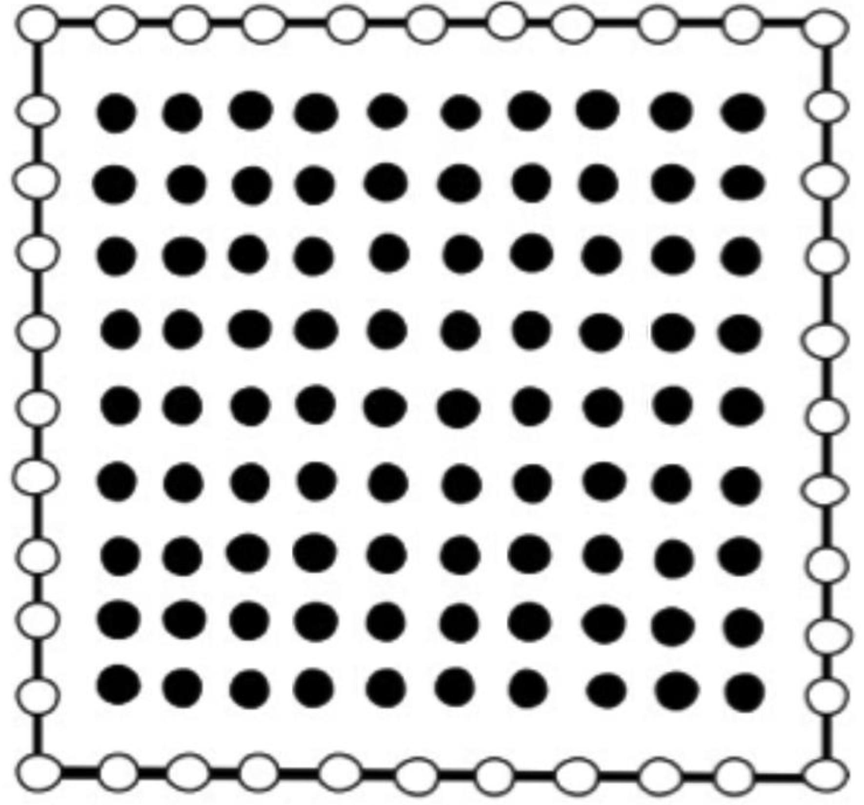
Figure 1. Boundary element model.

4. Numerical Results and Discussion

This study considers the generalized radial basis functions

R_{i} (r) = {(r^{2} + c^{2})}^{q}

r = |x - x_{i}|

, and the following parameters:

E = 210 G P a

v = 0.3

α = 0.000011

σ_{0} = 250 M P a

and

H = 0.05 E

. This study considered the computational domain, which has 40 boundary nodes and 90 internal nodes as illustrated in Figure 1.

This study also considered the reinforcing factors

\bar{α}

\bar{β}

and

({\bar{μ}}_{L} - {\bar{μ}}_{T})

, as well as the following anisotropic fibrous behavior

c_{i j k l} u_{k, l} = ⟦\bar{λ} ε_{k k} δ_{i j} + 2 {\bar{μ}}_{T} ε_{i j} + \bar{α} ({\bar{a}}_{k} {\bar{a}}_{m} ε_{k m} δ_{i j} + {\bar{a}}_{i} {\bar{a}}_{j} ε_{k k}) + 2 ({\bar{μ}}_{L} - {\bar{μ}}_{T}) ({\bar{a}}_{i} {\bar{a}}_{k} ε_{k j} + {\bar{a}}_{j} {\bar{a}}_{k} ε_{k i}) + \bar{β} {\bar{a}}_{k} {\bar{a}}_{m} ε_{k m} a_{i} a_{j}⟧

(i, j, k, m = 1, 2, 3), a \equiv (a_{1}, a_{2}, a_{3}), a_{1}^{2} + a_{2}^{2} + a_{3}^{2} (74)

The proposed methodology is applicable to a wide range of fibrous polymer nanomaterials issues, including nonlinear nonlocal elasticity. The numerical results demonstrate the computational performance of the proposed methodology, as shown in Table 1 and Table 2 below. The novel modified shift-splitting (NMSS) technique was applied to reduce memory and processing time requirements. Figures depict the numerical results, which highlight the effects of fractional and graded parameters on the thermal stresses of anisotropic fractional size and temperature-dependent fibrous polymer nanomaterials with nonlinear nonlocal elasticity.

Table 1. illustrates the CPU time and iterations number for regularized [43], generalized modified shift-splitting (GMSS) [44] and new modified shift-splitting (NMSS) [45] iterative methods at every discretization level, where the number of the equation is represented between parentheses. This table demonstrates the superiority of the NMSS over the regularized and GMSS approaches.

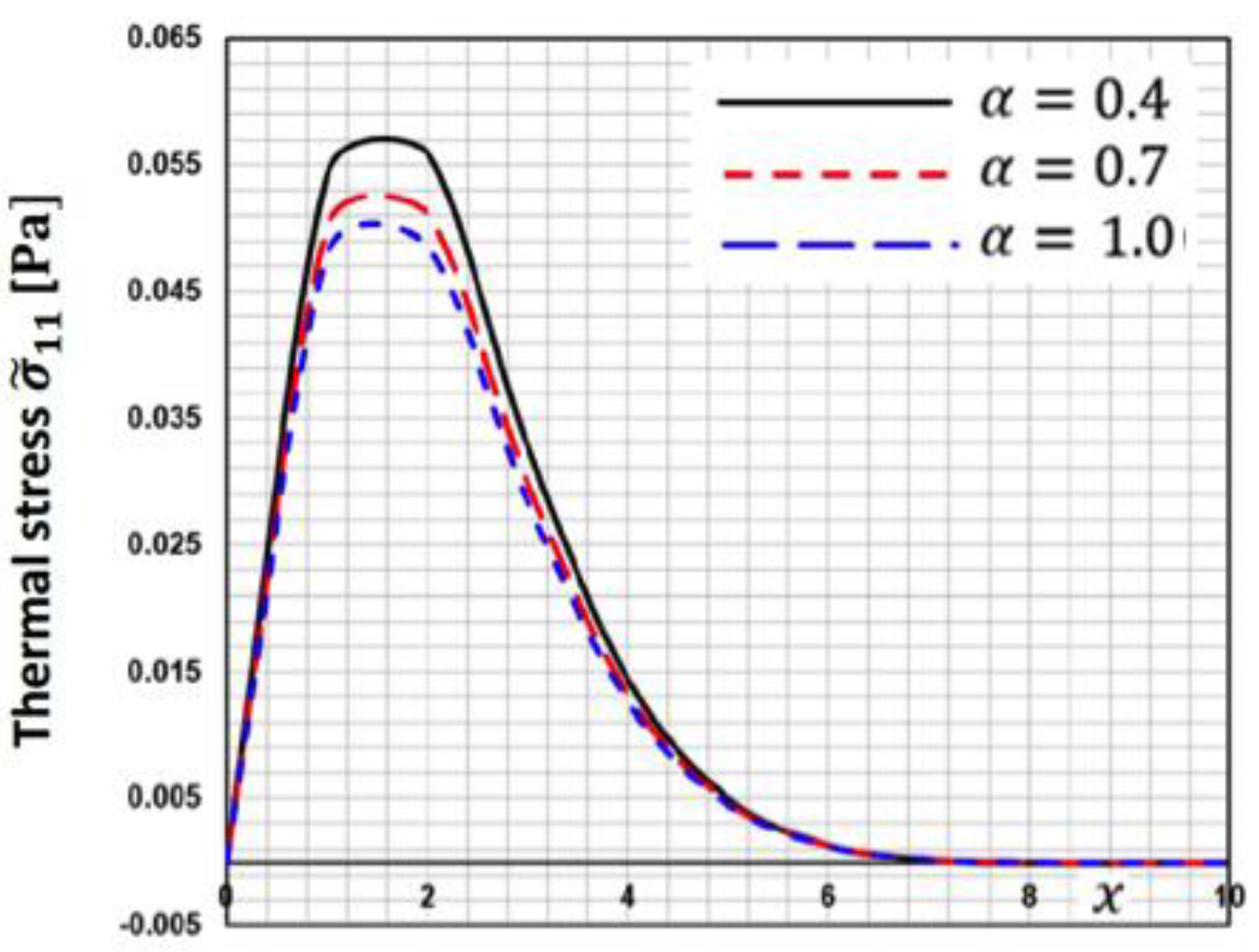
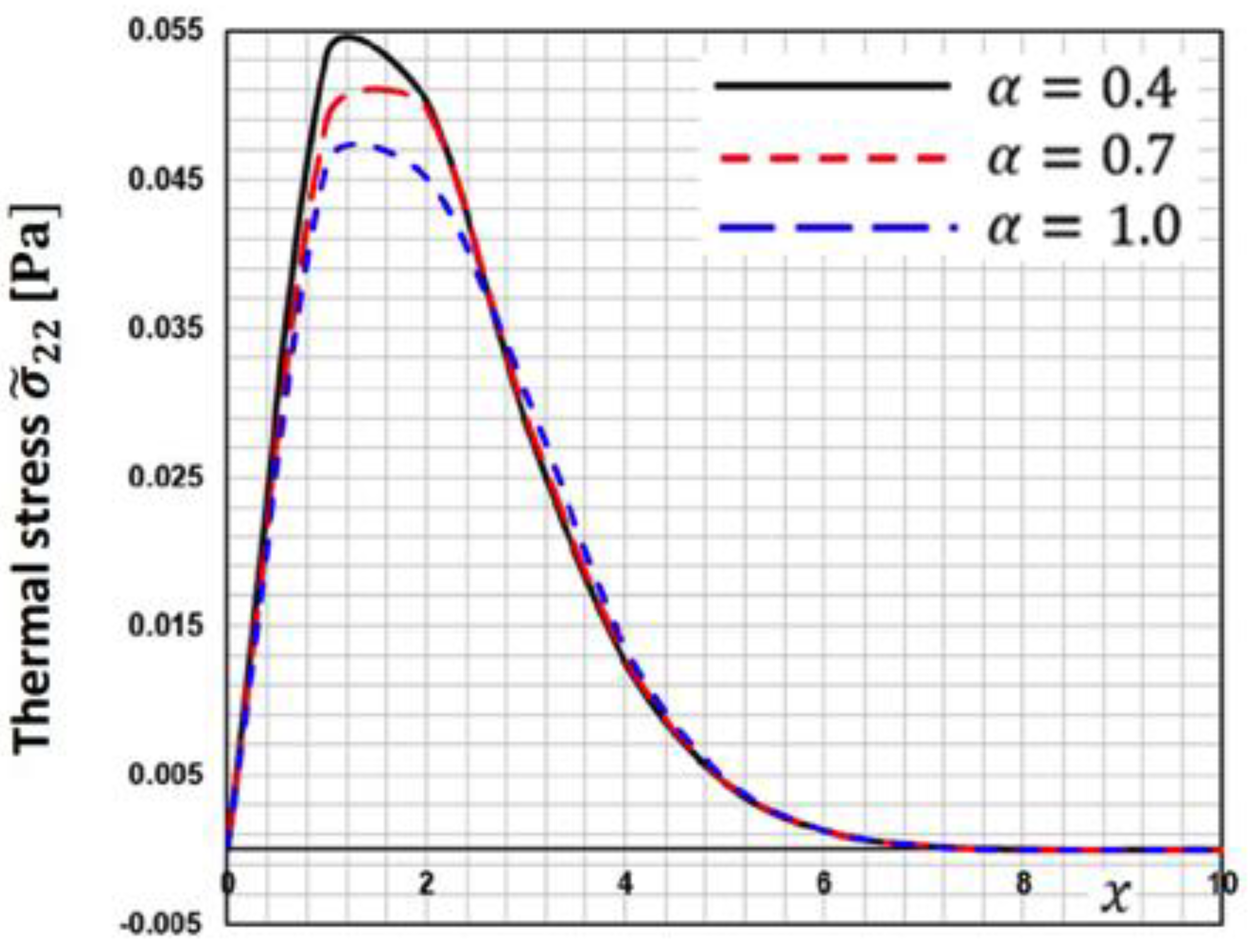
Figure 2 depicts the fluctuation of thermal stress

{\tilde{σ}}_{11}

along

x

-axis for various fractional order parameters

(α = 0.4, 0.7 a n d 1.0)

. This figure demonstrates that when the fractional order parameter increases, the thermal stress

{\tilde{σ}}_{11}

decreases.

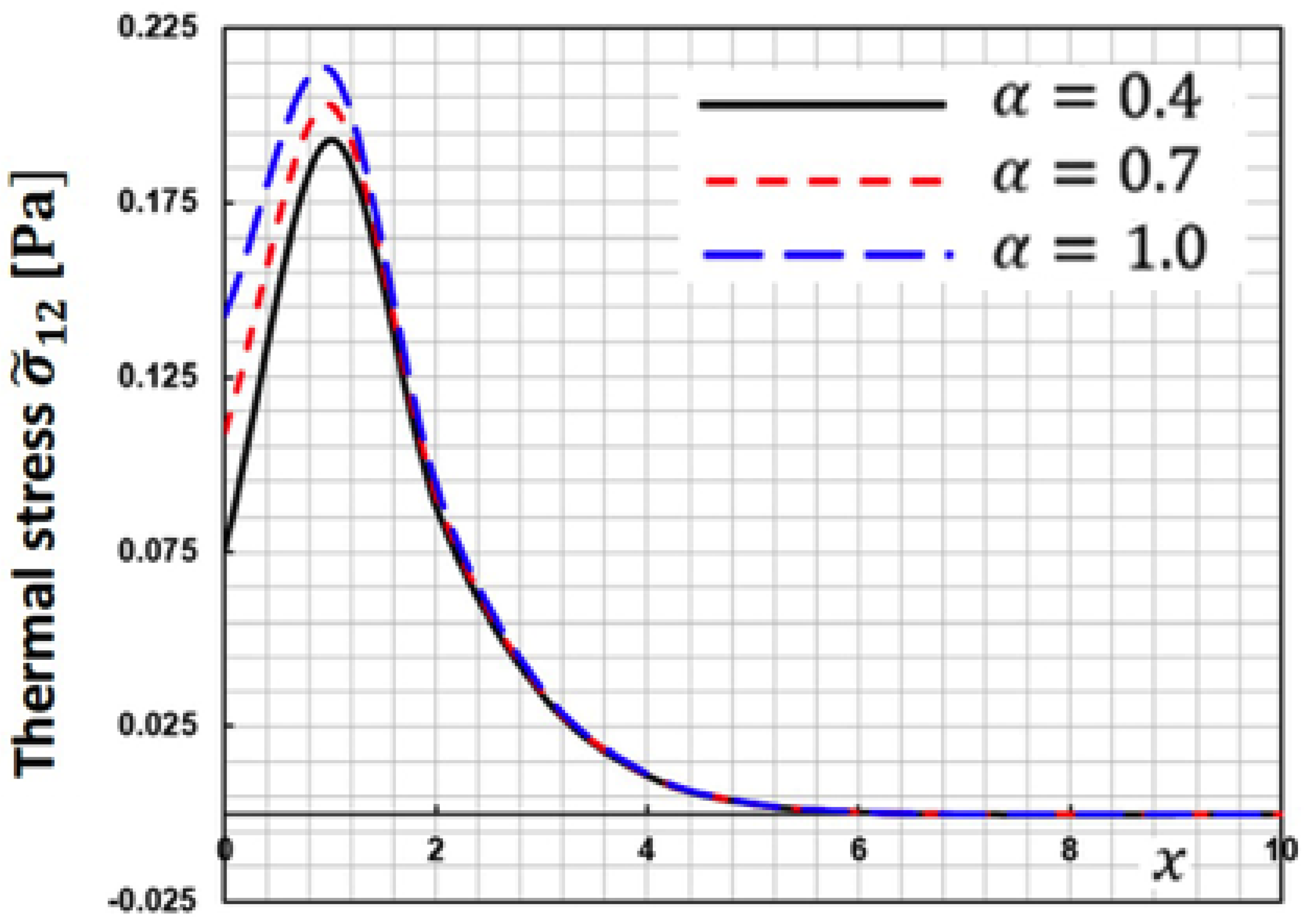
Figure 3 depicts the fluctuation of thermal stress

{\tilde{σ}}_{12}

along

x

-axis for various fractional order parameters

(α = 0.4, 0.7 a n d 1.0)

. This figure demonstrates that when the fractional order parameter increases, the thermal stress

{\tilde{σ}}_{12}

increases.

Figure 4 depicts the fluctuation of thermal stress

{\tilde{σ}}_{22}

along

x

-axis for various fractional order parameters

(α = 0.4, 0.7 a n d 1.0)

. This figure demonstrates that when the fractional order parameter increases, the thermal stress

{\tilde{σ}}_{22}

decreases.

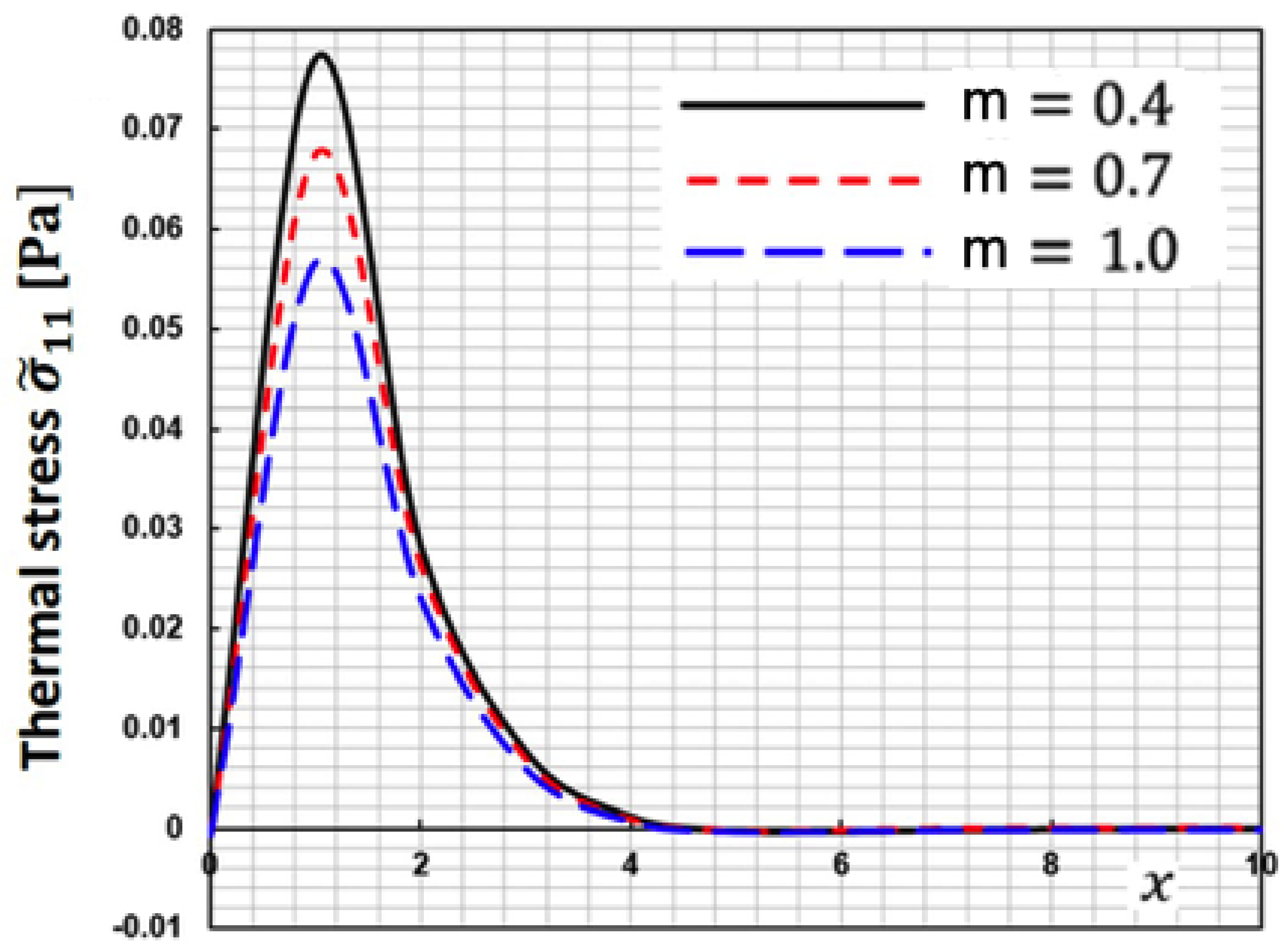
Figure 5 depicts the fluctuation of thermal stress

{\tilde{σ}}_{11}

along

x

-axis for various fractional order parameters

(m = 0.4, 0.7 a n d 1.0)

. This figure demonstrates that when the functionally graded parameter

m

increases, the thermal stress

{\tilde{σ}}_{11}

decreases.

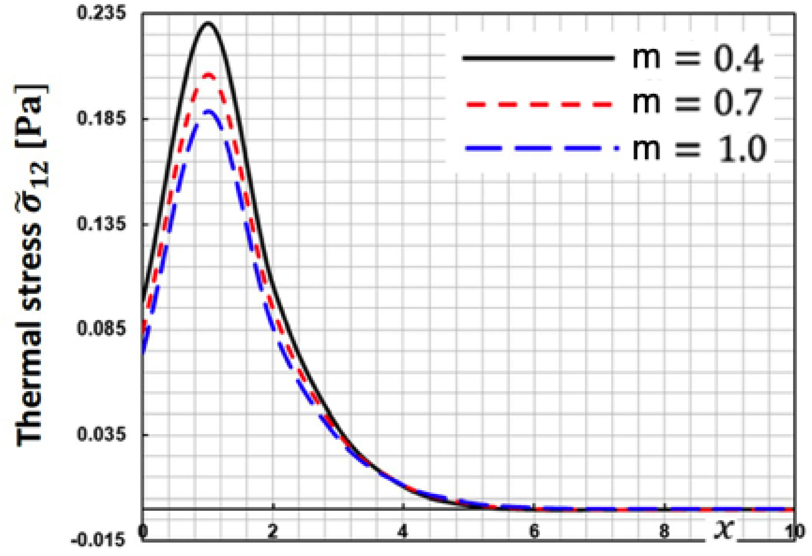
Figure 6 depicts the fluctuation of thermal stress

{\tilde{σ}}_{12}

along

x

-axis for various fractional order parameters

(m = 0.4, 0.7 a n d 1.0)

. This figure demonstrates that when the functionally graded parameter

m

increases, the thermal stress

{\tilde{σ}}_{12}

decreases.

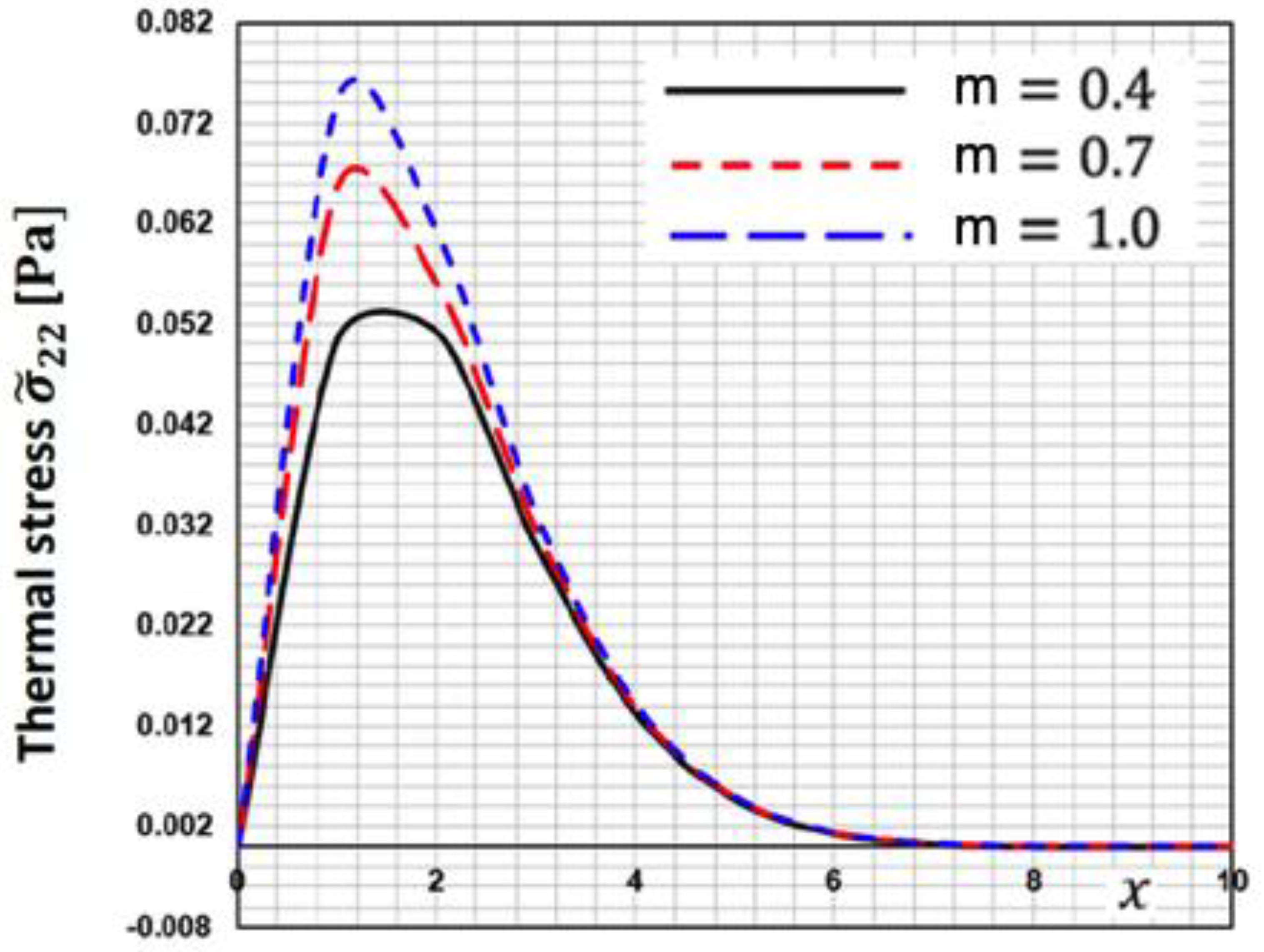
Figure 7 depicts the fluctuation of thermal stress

{\tilde{σ}}_{22}

along

x

-axis for various fractional order parameters

(m = 0.4, 0.7 a n d 1.0)

. This figure demonstrates that when the functionally graded parameter

m

increases, the thermal stress

{\tilde{σ}}_{22}

increases.

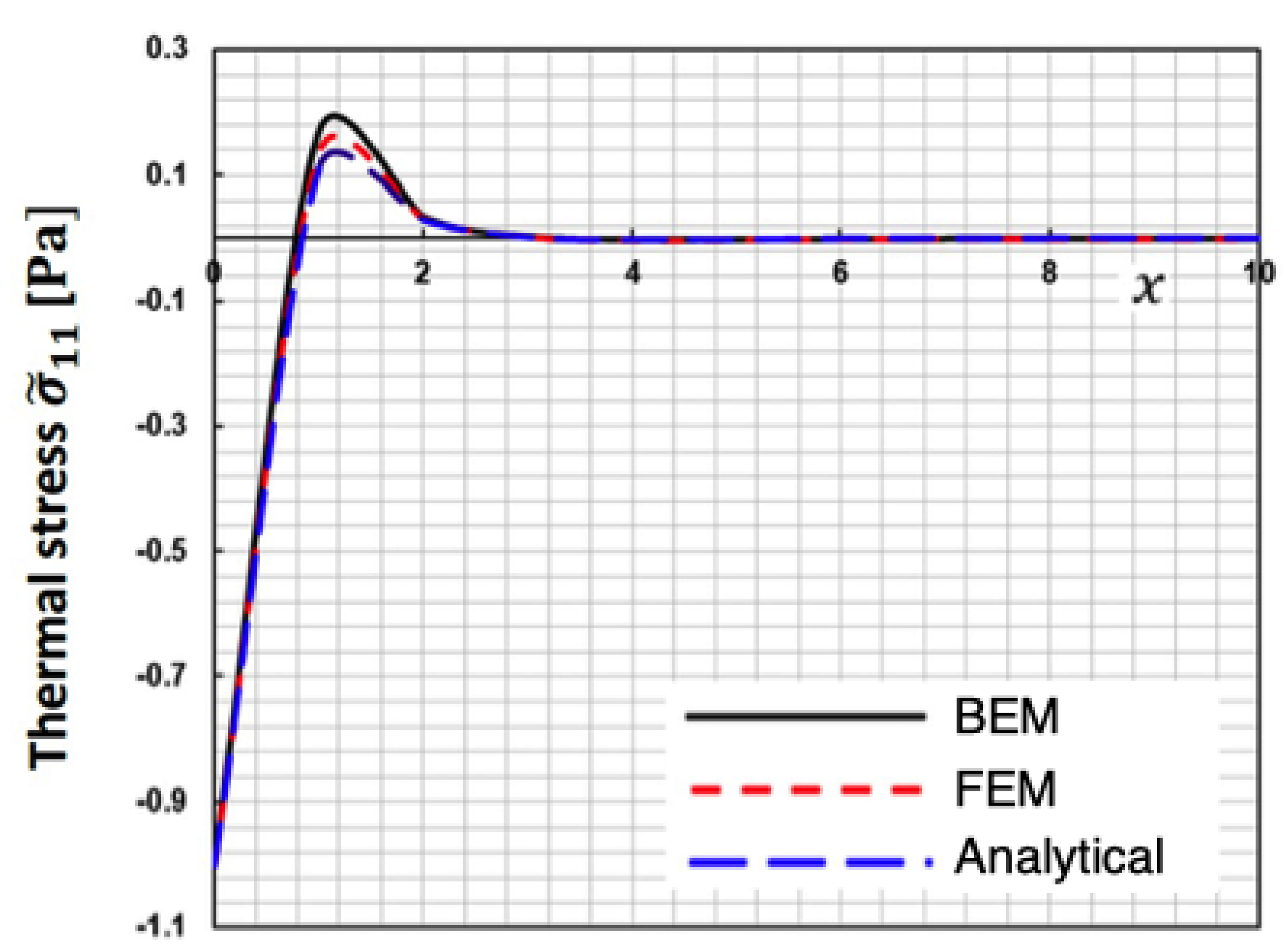
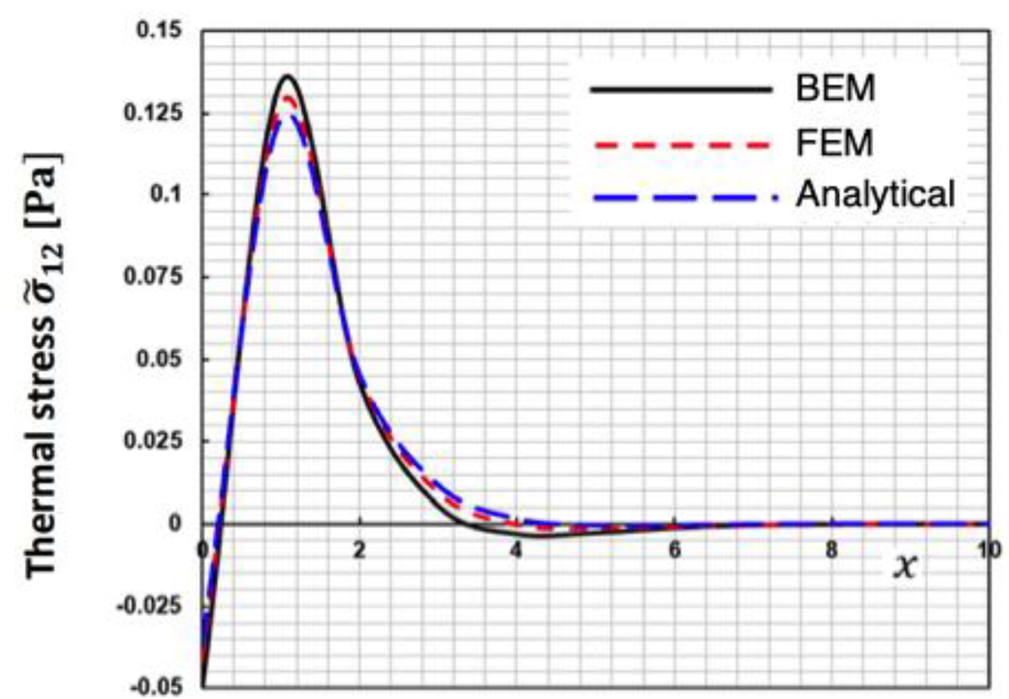
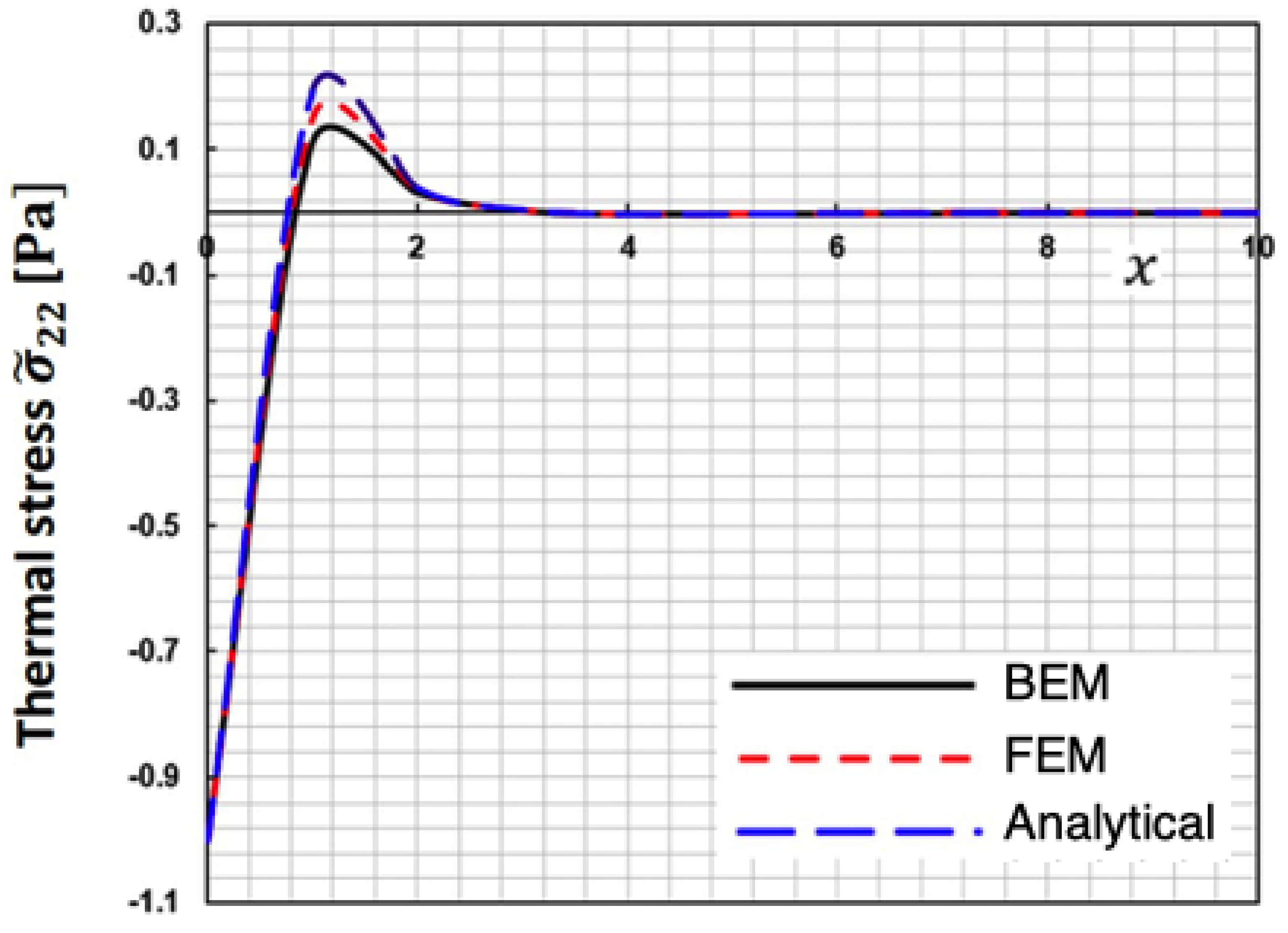
The current BEM approach strategy's validity and accuracy have not been shown by any published data. However, in the context of this current broad investigation, some works can be considered special cases.

Figure 8, Figure 9 and Figure 10 display the change of special case thermal stresses

{\tilde{σ}}_{11}

{\tilde{σ}}_{12}

and

{\tilde{σ}}_{22}

along the 𝒙-axis for the suggested BEM, finite element method (FEM) of Sidhardh, et al. [46] and analytical technique (Analytical) of Kumar and Mukhopadhyay [47], which are some special cases of our study. These figures show that the BEM results of the proposed technique match well with the LBM and FEM, validating the technique's validity and accuracy.

Table 2 compares computer resources needed to model anisotropic fractional size- and temperature- dependent fibrous polymer nanomaterials problems of nonlinear nonlocal elasticity for current BEM and finite element method (FEM). This table shows the effectiveness of our suggested BEM technique.

5. Conclusion

Nonlocal theories are gaining popularity because they can address difficulties that result in unphysical conclusions in traditional models. This paper describes a novel general boundary element method (BEM) solution for anisotropic fractional size- and temperature-dependent fibrous polymer nanomaterials with nonlinear nonlocal elasticity. This comprehensive BEM solution incorporates two approaches: the BEM solution for size-dependent nanomaterials and the solution for nonlocal elastic problems. The nonlocal elastic technique separates the displacement field into complimentary component and particular components. The overall displacement is obtained using the boundary element technique, which solves a Navier type problem, whereas the individual displacement is derived using local radial points. The New Modified Shift-Splitting (NMSS) approach, which reduces memory and processing time requirements, has been used to solve linear systems created by BEM. Figures demonstrate the numerical findings, which show the impacts of fractional and graded parameters on the thermal stresses of anisotropic fractional size- and temperature-dependent fibrous polymer nanomaterials with nonlinear and nonlocal elasticity. The numerical findings suggest that the proposed methodology is consistent and efficient. Our current numerical results may be of interest to polymer scientists and engineers. It is possible to conclude that our research is also very important for polymer applications such as food packaging, phones, soda and water bottles, films, agriculture, biomedical devices, coating, paints, blending, airplanes, textile fibers, automotive, consumer goods, industrial, recreational vehicles, effective actuators, fluorescence imaging, photodynamic therapy, hydrogels, electronic devices, engineering resins and polyolefins, and computers, among others.

Funding

The authors did not receive support from any organization for the submitted work.

Data Availability Statement

All data generated or analysed during this study are included in this published article.

Conflicts of Interest

The authors declare no conflict of interest.

Nomenclature

$α$	Thermal expansion	$k_{i j}$	Pseudo mean curvature tensor
$Γ$	Thermal shear strain	$l$	Internal length of considered material
$Γ$	Boundary	$\bar{m}$	Couple-traction
$δ_{α β}$	Kronecker delta function	$M$	Monomials number
$ε_{i j}$	Strain tensor	$M_{i}$	True couple-stress vector
$η$	Couple-stress parameter	$M_{i j}$	Pseudo couple-stress tensor
$σ_{0}$	Yield stress	$m$	Functionally graded parameter
$σ_{α β}$	Total force-stress tensor	$n$	Outward unit normal vector
$σ_{(α β)}$	Symmetric force-stress tensor	$N$	Nodes number
$σ_{[α β]}$	Skew-symmetric force-stress tensor	P	Pressure
$Ω$	Rotation	$p^{*}$	Point couple kernel function
$Ω_{f}$	Spherical region	$P_{j} (x)$	Monomials
$c & q$	Shape parameters	$Q$	External heat source
$\bar{c}$	Heat capacity	$r$	Euclidian distance
$c^{*}$	Point force kernel function	$R$	Radius of spherical region
$C_{i j k l}$	Fourth-order constant stiffness tensor	$R_{i} (r)$	$= {(r^{2} + c^{2})}^{q}$ Radial basis function
$E$	Young's modulus	$T_{m i}$	Traction
$F_{i}$	Body force vector	$u$	Displacement vector
$H$	Strain hardening	$U_{m i}$	Kelvin fundamental solution
I	Identity tensor	$v$	Poisson's ratio
$k_{B}$	Boltzmann’s constant	$x$	Evaluation point
$k_{i}$	Mean curvature vector	$x_{i}$	Center point
		$x^{'}$	Field point

References

J. Ghanbari and R. Naghdabadi. Multiscale nonlinear constitutive modeling of carbon nanostructures based on interatomic potentials, CMC-Computers, Materials & Continua, 10 (2009) 41-64.
Chakrabarty and T. Çağin. Computational studies on mechanical and thermal properties of carbon nanotube based nanostructures, CMC-Computers, Materials & Continua.7 (2008) 167-190. [CrossRef]
S. N. Cha, J. S. Seo, S. M. Kim, H. J. Kim, Y. J. Park et al., Sound-driven piezoelectric nanowire-based nanogenerators, Advanced Materials. 22 (2010) 4726-4730. [CrossRef]
S. Zhang, B. Gu, H. Zhang, X. Q. Feng, R. Pan et al., Propagation of Love waves with surface effects in an electrically-shorted piezoelectric nano film on a half-space elastic substrate, Ultrasonics, vol. 66 (2016) 65-71. [CrossRef]
F. Akyildiz and J. M. Jornet, Electromagnetic wireless nanosensor networks, Nano Communication Networks, vol. 1, no. 1, pp. 3-19, 2010. [CrossRef]
He, X. Qi, Y. Miao, H. L. Wu, N. He et al., Application of smart nanostructures in medicine, Nanomedicine, vol. 5, no. 7, pp. 1129-1138, 2010. [CrossRef]
Y. Al-Hossain, F. A. Farhoud and M. Ibrahim, “The mathematical model of reflection and refraction of plane quasi-vertical transverse waves at interface nanocomposite smart material,” Journal of Computational and Theoretical Nanoscience, vol. 8, no. 7, pp. 1193-1202, 2011. [CrossRef]
L. Zhu and X. J. Zheng, Stress field effects on phonon properties in spatially confined semiconductor nanostructures, CMC-Computers, Materials & Continua.18 (2010) 301-320.
Fahmy (2021). A new boundary element formulation for modeling and simulation of three-temperature distributions in carbon nanotube fiber reinforced composites with inclusions. Mathematical Methods in the Applied Science. [CrossRef]
Fahmy. A new BEM modeling algorithm for size-dependent thermopiezoelectric problems in smart nanostructures. CMC-Computer, Materials & Continua, 69 (2021) 931-944,. [CrossRef]
A Fahmy‏ Fractional Temperature-Dependent BEM for Laser Ultrasonic Thermoelastic Propagation Problems of Smart Nanomaterials‏. Fractal Fract. 2023, 7(7), 536. [CrossRef]
Sudak LJ. Column buckling of multiwalled carbon nanotubes using nonlocal continuum mechanics. J Appl Phys 2003;94:7281-7. [CrossRef]
Wang Q. Varadan VK. Application of nonlocal elastic shell theory in wave propagation analysis of carbon nanotubes. Smart Mater Struct 2008;16: 178-90. [CrossRef]
Filiz S, Aydogdu M. Axial vibration of carbon nanotube heterojunctions using nonlocal elasticity. Comp Mater Sci 2010;49:619–27. [CrossRef]
Hu Yan-Gao, Liew KM, Wang Q. He XQ, Yakobson BI. Nonlocal shell model for elastic wave propagation in single and double walled carbon nanotubes. J Mech Phys Solids 2008:56:3475–85. [CrossRef]
Eringen AC. Theory of nonlocal elasticity and some applications. Res Mech.
Kröner E. Elasticity theory of materials with long range cohesive forces. Int Solids Struct 1967; 3: -31–42. [CrossRef]
Kunin IA. The theory of elastic media with microstructure and the theory of dislocation. In: Kröner E, editor. Mechanics of Generalized Continua; 1968.
Krumhansl JA. Some consideration on the relations between solid state physics and generalized continum mechanics. In: Kröner E, editor. Mechanics of Generalized Continua; 1968.
Edelen DGB, Laws N. On the thermodynamics of systems with nonlocality. Arch Rationale Mech Anal 1971;43:24-35. [CrossRef]
Edelen DGB, Green AE, Laws N. Nonlocal continuum mechanics. Arch Rationale Mech Anal 1971;43:36-44.
Eringen, Edelen DGB. On nonlocal elasticity. Int J Eng Sci 1972; 10: 233–48.
Eringen AC, Kim BS. Stress concentration at the tip of a crack. Mech Res Eringen AC, Kim BS. Stres 1974;1:233–7. [CrossRef]
Eringen AC, Speziale CG, Kim BS. Crack tip problem in nonlocal elasticity. J Mech Phys Solids 1977:25:339-55. [CrossRef]
Eringen AC. Line Crack subjected to shear. Int J Fract 1978;14: 367–79. [CrossRef]
Eringen AC. Line Crack subjected to anti-plane shear. Eng Fract Mech 1979;12:211–9. [CrossRef]
Gao J, Dai TM. On the study of a penny-shaped crack in nonlocal elasticity. Acta Mech Solids Sin 1989; 2: 253–69.
Minghao Z, Changjun C, Yuanjie L, Guoning L, Shishan Z. The method of analysis of crack problem in three dimensional non-local elasticity. Appl Math Mech 1999; 20. [CrossRef]
Eringen AC. Edge dislocation in nonlocal elasticity. Int J Eng Sci 1977; 15: 177-83. [CrossRef]
Eringen AC. Screw dislocation in nonlocal elasticity. J Phys D Appl Phys 1977; 10: 671–8. [CrossRef]
Lazar M, Maugin GA, Aifantis EC. On a theory of nonlocal elasticity of biHelmholtz type and some applications. Int J Solids Struct 2006;43:1404-21. [CrossRef]
Povstenko YZ, Kubik I. Concentrated ring loading in a nonlocal elastic medium. Int J Eng Sci 2005;43:457-71. [CrossRef]
Artan. The nonlocal solution of the elastic half plane loaded by a couple. Int J Eng Sci 1999;37:1389-405. [CrossRef]
Michael Rubinstein and S. Panyukov. Elasticity of Polymer Networks. Macromolecules 35(17):6670-6686. [CrossRef]
Hematiyan, M.R. Exact transformation of a wide variety of domain integrals into boundary integrals in boundary element method. Commun. Numer. Methods Eng. 2008, 24, 1497–1521. [CrossRef]
Hadjesfandiari, A.R.; Dargush, G.F. Fundamental solutions for isotropic size-dependent couple stress elasticity. Int. J. Solids Struct. 2013, 50, 1253–1265. [CrossRef]
Lazar M, Maugin GA, Aifantis EC. On a theory of nonlocal elasticity of biHelmholtz type and some applications. Int J Solids Struct 2006;43:1404-21. [CrossRef]
Polizzotto C, Fushi P, Pisano AA. A strain-difference-based nonlocal elasticity model. Int J Solids Struct 2004;41:2383-401. [CrossRef]
Liu GR, Gu YT. A meshfree method: meshfree weak-strong (MWS) form method for 2-D solids. Comput Mech 2003; 33: 2–14. [CrossRef]
Schwartz, N.T. Niane, R. Kouitat Njiwa. A simple solution method to 3D integral nonlocal elasticity: Isotropic-BEM coupled with strong form local radial point interpolation. Engineering Analysis with Boundary Elements. Volume 36, Issue 4, April 2012, Pages 606-612. [CrossRef]
Brebbia CA, Dominguez J. Boundary Elements. An Introductory Course. Computational Mechanics Publications; 1992.
Liu GR, Gu YT. A local radial point interpolation method (LRPIM) for free vibration analyses of 2-D solids. J Sound Vib 2001;246:29-46. [CrossRef]
Badahmane,A.(2020).Regularized preconditioned GMRES and the regularized iteration method. Applied Numerical Mathematics, 152, 159–168. [CrossRef]
Huang, Z. G., Wang, L. G., Xu, Z., Cui, J. J. (2017). The generalized modified shift-splitting preconditioners for nonsymmetric saddle point problems. Applied Mathematics and Computation, 299, 95–118. [CrossRef]
Ardeshiry, M., Goughery, H.S. & Pour, H.N. New modified shift-splitting preconditioners for non-symmetric saddle point problems. Arab. J. Math. 9, 245–257 (2020). [CrossRef]
Sidhardh, S.; Patnaik, S.; Semperlotti, F. Thermodynamics of fractional-order nonlocal continua and its application to the thermoelastic response of beams. European Journal of Mechanics / A Solids 2021, vol. 88, pp. 104238. [CrossRef]
Kumar, H. and Mukhopadhyay, S.. Size-dependent thermoelastic damping analysis in nanobeam resonators based on Eringen’s nonlocal elasticity and modified couple stress theories, 2022, Volume 29, Issue 7-8, pp. 1510–1523. [CrossRef]

Figure 1. Polymer chain's elasticity configuration of

N

Kuhn segments of length

b

, with end-to-end vector

R

, and contours length

L = N b

Figure 1. Polymer chain's elasticity configuration of

N

Kuhn segments of length

b

, with end-to-end vector

R

, and contours length

L = N b

Figure 2. Thermal stress

{\tilde{σ}}_{11}

distribution along the

x