Submitted:
24 April 2024
Posted:
25 April 2024
You are already at the latest version
Abstract
Direct Energy Deposition (DED) is a versatile and efficient method in metal additive manufacturing. However, humping, caused by abnormal dynamics in the melt pool (MP), poses a significant threat to the geometric integrity of manufactured products. Current state-of-the-art (SOTA) methods primarily detect humping by analyzing late-stage spatial abnormalities, such as MP detachment. This approach is fundamentally reactive, leading to a tendency to miss early humping spatiotemporal dynamics, like cyclic elongation of the MP. This study introduces a novel, proactive indicator named VIMPS (Variability of Instantaneous MP Solidification-Front Speed), a physics-based tool designed to quantify early abnormal fluctuations in MP solidification speed. The experiments demonstrate VIMPS correlation with humping-induced geometric inaccuracies. By capturing early spatiotemporal dynamics of the MP, VIMPS reduces detection latency by 30 seconds compared to existing SOTAs that focus solely on spatial abnormalities. This significant improvement transforms detection from reactive to proactive, providing the time needed for corrective actions to enhance the overall productivity and quality of the DED process.
Keywords:
monitoring
; additive manufacturing
; direct energy deposition
; proactive
; solidification front
; spatiotemporal
1. Introduction
Direct energy deposition (DED) stands out among additive manufacturing (AM) technologies due to its high productivity of geometries with near-to-optimal shapes. The capability of multi-axis material delivery as powder or wire enables the creation and repair of complex geometries, large-scale parts, and multi-grade materials, aligning with the demands of aerospace applications [1,2,3]. This advantage of material delivery in DED comes with significant challenges. Unlike powder bed processes, where the powder is laid statically, the DED material’s dynamic delivery complicates the heat dissipation [4,5]. The continuous and localized addition of material generates varying heat intensities and gradients, leading to a complex thermal profile within the heat-affected zones. This complexity in heat management can result in various defects and the absence of consistent and standardized process output characteristics. The non-uniform cooling, the heat accumulation, and the re-melting of built layers during the disposition of new ones lead to micro and macro defects such as geometric and dimensional distortion, surface and internal cracks, and porosity formation [6]. Consequently, a large body of literature focuses on developing different monitoring and control systems to improve the reliability and repeatability of DED processes [7].
Humping is a phenomenon that significantly reduces the geometrical accuracy of the produced products. Figure 1a shows a severe manifestation humping, demonstrating the formation of crests and valleys that contribute to the characteristic wavy structure. During humping, the melt pool goes through a series of abnormal solidification dynamics (i.e., modes). Transitioning between these different modes depends on the humping severity, as shown in Figure 1. Panels (b to f) showcase the different melt pool modes associated with humping, with the severity increasing progressively from (b) to (f). Additionally, within each panel, time progresses from the top to the bottom (e.g., b.1 precedes b.2). Starting with the normal mode, in Figure 1b.1 and 1.b.2, the melt pool (MP) shows a temporally invariant shape. This temporal invariant shape implies that the solidification front (SF) speed matches the laser speed. Thus, the relative velocity between the laser and solidification front at the melt pool tail is almost zero. The initial stage of humping starts with the MP elongation mode. In this mode, the MP shows cyclic behavior, alternating between long (Figure 1c.1) and short melt pools (Figure 1c.2). This variation in melt pool size indicates inconsistent solidification front velocity direction (SFD), which is the direction of the relative velocity between the solidification front and the scanning speed, as shown by the orange arrows in Figure 1c. A negative SFD means that the solidification front is moving away from the laser, and the liquid is accumulating at the MP tail, as shown in Figure 1c.1. Conversely, a positive SFD indicates liquid solidifing at the tail, causing a shorter MP. Despite this fluctuation in the SFD, the degradation of geometric accuracy is minimal during the early humping stage (i.e., elongation mode).
As the severity of humping intensifies, the process transitions from the elongation mode to the swelling mode. A significant volume of liquid accumulates at the MP’s tail (Figure 1d.1) and solidifies locally, leading to crest formation at the tail (Figure 1d.2). When the elongation is excessive, the detachment mode is activated. The MP tail is detached and forms an isolated liquid volume (Figure 1e.2), further contributing to crest formation (Figure 1e.3).
During swelling mode, the continuous formation of these crests deteriorates the printed part’s geometrical accuracy rendering it wavy (Figure 1f.1). When the surface is wavy, late humping symptoms (i.e., tilting mode) are observable. The MP follows a distorted path (i.e., wavy trajectory); thus, it starts to tilt; see the change in the MP orientation indicated by the blue line in Figure 1f.2 to Figure 1f.4.
The current literature offers various contradictory mechanisms that trigger the elongation and swelling mode. Some hypothesize a relation between powder density gradients in the gas-powder jet and humping creation. They assume that the powder gradient can cause protrusion growth [9]. Such protrusions are similar to the swelling in Figure 1d.1 and thus can also lead to the formation of the humping wavy surface in Figure 1. (a). However, humping is not exclusive to powder-based AM processes but is also common in non-power-based processes such as welding [10,11,12]. In welding literature, humping is often related to factors such as strong forward flow momentum and limited backfilling. The process conditions that trigger these factors are still unclear. In keyhole printing, with high energy intensity and deep depression in the laser-material interaction zones, some hypothesize that the lateral oscillation of the keyhole triggers humping [13,14]. However, humping is not exclusive to the high-energy-intensity keyhole printing mode but is also observed for conduction-mode welding with lower energy intensity and shallow melt pools. Gullipalli et al., 2023 have even recently shown that reducing heat input in DED (i.e., moving from keyhole to conduction mode printing conditions) can aid in activating humping [15]. These contradictory recommendations and explanations arise from the complex non-linear interaction of physics in metal welding and printing. Thus, generalizations of these explanations or guidelines will always be doubtful, reducing the reliability of offline energy input optimization and emphasizing the need for real-time printing monitoring systems.
Instead of energy input optimization, the industry adopts energy management optimization. Energy management can be done by active cooling [16,17], or interlayer dwelling, with the latter being the more common strategy. Interlayer dwells pause the printing for a predetermined dwell time (DT) after a predetermined continuous deposition time (CDT), allowing the part to cool down and reach a predetermined temperature before resuming printing [18,19]. If achieved, optimal energy management is capable of keeping the melt pool in its normal state (Figure 1b), effectively preventing humping. However, predetermining DT and CDT is a considerable optimization problem. For example, it has been shown that the optimal CDT varies depending on the printed part geometry and the current build height [20]. Frequent stopping or unnecessarily prolonged dwell reduces productivity and subjects the part to unnecessary thermal cycles, potentially degrading quality [21,22]. Conversely, excessive delays in stopping (i.e., too long CDT) may lead to irreversible geometric inaccuracies, rendering the part as scrap unless hybrid additive-subtractive manufacturing techniques are available. Therefore, identifying the optimal stopping time that maximizes the CDT is crucial, highlighting the need for advanced real-time monitoring technologies.
While there are numerous studies dedicated to online monitoring solutions for detecting humping onset in additive manufacturing, the majority are reactive rather than proactive. This is because they have focused on humping late spatial symptoms rather than early spatiotemporal dynamics [23,24,25]. For instance, [24] detects humping when the melt pool is spatially detached into two separate liquid volumes (i.e., the detachment mode illustrated in Figure 1e.2). At this stage, geometric inaccuracies caused by humping have already manifested and may lead to part scraping. Therefore, proactive monitoring of humping is crucial to provide enough time to take action to prevent irreversible geometric defects.
The principle contribution of this study is detecting the early elongation mode of humping. In contrast to the detachment mode, the elongation detection necessitates the simultaneous consideration of spatial and temporal (i.e., spatiotemporal) dynamics. In other words, in contrast to monitoring the swelling state illustrated in Figure 1e.2, This work aims at simultaneously investigating the spatiotemporal dynamic of elongation mode to detect humping (i.e., the variation between Figure 1c.1 and c.2). The distinct elongation and swelling modes physics is at the core of the proposed approach novelty, allowing it to:
- Transform from reactive to proactive humping detection.
- Transform humping detection from spatial (i.e., detachment) to spatiotemporal (i.e., elongation) abnormalities.
- Practically track the variability in solidification front dynamics.
The structure of this study is organized as follows: Section 2 describes the experimental setup and test matrix utilized for collecting the infrared videos. Section 3 focuses on interpreting and processing the data to calculate the proposed humping indicator (VIMPS). Section 4 empirically confirms the superiority of VIMPS compared to current state-of-the-art approaches.
2. Experimental Setup
Experiments were done on a 3kW TRUMPF TruDiode laser integrated with a six-axis CNC gantry. This system incorporated Reis Lasertec optics, an ILT powder nozzle, and a Sulzer-Metco TWIN-10 feeder. A 125 mm collimation lens, a 150 mm focal lens, a 600 µm fiber, a laser of wavelength of 950 nm, and a spot size of D = 2.6 mm were used. Figure 2 shows the laser profile used. In this study, austenitic nickel-chromium stainless steel powder was used; it has a nominal particle size distribution between -45 and +11 µm and a chemical composition of Fe 17Cr 12Ni 2.5Mo 2.3Si 0.03C. Circular builds of 25 mm in both height and diameter were constructed under varied printing conditions, as detailed in Table 1. Three parts were printed using combinations of two laser powers P, and two traverse speeds v. All prints were made with an 8 g/min powder flow rate.
For melt pool monitoring, a med-wave infrared MWIR camera (i.e., FLIR SC8300) is used. The MWIR option was selected to ensure the capture of low-temperature regions, such as the melt pool tail, which cannot be captured by a normal VIS camera (i.e., a camera only sensitive to visible light). This is because visible light is mainly emitted by objects at extremely high temperatures [26]. The camera was equipped with a 50 mm focal lens with a 1-inch extension tube to achieve the desired field of view (FOV) of 5 mm x 3.5 mm. The camera was operated at a frame rate of 233 Hz and a resolution of 256 x 180 pixels. These settings were selected so that the sampling frequency was adequate to capture the humping dynamics. To allow for continuous monitoring and to negate any relative movement between the melt pool and the camera, the camera was directly mounted on the laser head, as shown in Figure 3b. The table was rotated while the head moved in the positive Z direction, as shown in Figure 3. The combined head and table motion leads to a continuous helical printing path. After printing, the as-printed parts are imaged using a ZEISS Smartzoom 5 automated digital microscope to assess the geometrical accuracy qualitatively (i.e., topography).
3. Signal Processing
3.1. Pixel Intensity Physical Interpretation
The present study collects the melt pool infrared signature as a series of 2D images throughout the printing duration. These sequential images provide a comprehensive overview of the melt pool spatiotemporal variations. Figure 4 shows a single frame; the top part shows the large field of view (The top image shows a zoomed out FOV, not the processed FOV in the developed approach) of the entire cylinder, while the bottom part zooms in on the heat-affected zone (HAZ) and the melt pool. It should be noted that despite its higher temperature, the melt pool in Figure 4, marked in red, exhibits a darker appearance, indicative of lower pixel intensity. This phenomenon can be explained by the variations in emissivity associated with different phases of the material, which affect its heat radiation. According to the Stefan-Boltzmann law, the total radiation (Prad) emitted by a body is a function of both its temperature (Temp) and its emissivity (ϵ), expressed as Prad = σϵATemp4, where σ represents the Stefan-Boltzmann constant. In the case of stainless steel, the liquid phase exhibits a lower emissivity compared to its solid counterpart [27] especially when the solid is oxidized [28]. Consequently, the darker appearance of the melt pool in Figure 4 suggests that the decreased emissivity in the liquid state has a more pronounced effect than the increased temperature. Such observation can be confirmed by analyzing the sequence of the melt pool’s image after the deactivation of the laser shown in Figure 5. During such a sequence of images, the melt pool is solidifying; thus, its temperature consistently declines. Notably, in Figure 5, the pixel intensity of the melt pool initially increases, reaching its peak around time t = 304 seconds, followed by a reduction at t = 307 seconds. This temporary increase in pixel intensity during the solidification can be attributed solely to changes in emissivity as the material transitions from liquid to solid phases. Consequently, this explains that the lower pixel intensity of the melt pool is due to its lower emissivity. This pattern aligns with observations reported in [29], where steel displayed similar radiative characteristics during solidification in an Argon environment.
3.2. Physics-Based Indicator
This Section outlines the proposed methodology for calculating the variability of the instantaneous MP solidification-front speed (VIMPS) indicator from the raw collected IR videos. VIMPS is designed to quantify the Variability in SFD during elongation and swelling modes. The proposed method starts by defining a region of interest (ROI) around the melt pool, as shown in Figure 6. Within this ROI, for every time step, three principal indicators are computed: (1) Average Pixel Intensity (API), (2) Rolling Variance of API (APIRV), and (3) Rolling Mean of API (APIRM). These indicators are instrumental in calculating the VIMPS indicator. The following sections detail the computation and rationale behind these three critical indicators.
The API reflects the dominance of the solid phase over the liquid phase in the composition within the ROI. It is designed to have an inverse and positive correlation with the MP size and the SFD, respectively, as shown in Table 2. It can be calculated at a specific time step as follows:
where and are the width and height of the ROI, respectively. represents the Pixel Intensity at coordinates in the IR-captured video frame. According to section 3.1, is higher for solidified stainless-steel powder used in this study. Consequently, API is higher when the solid phase dominates the ROI composition. For example, Figure 6 shows the API variations during the accumulation and solidification through one elongation mode cycle. In Figure 6a, when the melt pool is small, the ROI composition is dominated by the solid phase; thus, API is high, as shown in Figure 6d. Driven by limited backfilling and dominant forward flow, as illustrated in Figure 6b, liquid accumulates within the melt pool tail, and the SFD switches to the negative direction, denoting the onset of elongation’s mode. This elongation mode shifts the ROI composition towards the liquid phase, reducing the API, as Figure 2(d) illustrates. This API drop is due to the liquid’s lower . Upon reaching maximal extension, the MP undergoes rapid cooling, reversing the SFD, and leading to a localized solidification in the tail, as shown in Figure 6c. This solidification domainates the ROI and increase the , thus increasing the API. Such an accumulation-solidification cycle, summarized in Table 2, will repeat throughout the elongation mode, fluctuating SFD between positive and negative values. Such fluctuations are reflected on the API, leading to the cycle shown in Figure 6c. The cycle amplitude (A) and period (T) depend on the humping intensity; small T and large A indicate intense humping. In contrast, during the normal mode (i.e., no humping), as shown by the horizontal straight line in Figure 6d, the API remains unchanged (i.e., T → ∞, A →0) as SFD will remain zero. The subsequent steps to calculate the VIMPS indicator are essential signal-processing steps designed to minimize noise, enhance robustness, and streamline decision-making processes.
Instead of calculating the cycle amplitude (A) and period (T) to quantify humping intensity, the Rolling Variance of API (APIRV) will be used. APIRV calculates the variance in API as follows:
where, is the rolling window duration, is a time step within the rolling window, is the current time step. In this study was set to 2 sec, and is the API rolling mean defined per Equation 3. Compared to the (A, T), APIRV is more straightforward to calculate as it does not involve frequency analysis and still provides the information needed for humping detection. Small (T) and large (A) will be reflected as high APIRV Thus, a sudden increase in APIRV indicates the MP transitioning from normal to elongation mode.
The Rolling Mean of API (APIRM) is also used to enhance the robustness of APIRV by making it less sensitive to variances that are unrelated to elongation and is calculated as follows:
APRIVxM, the more robust version of APRIV, is calculated as follows:
In the calculated APRIVxM, since APIRM is low at early layers (i.e., low total heat input), it dampens the APIRV. This dampening improves robustness against unrelated variances, particularly noticeable during the initial layers, where APIRV increase is not attributable to elongation but to initial MP formation and heat dissipation into the substrate.
Finally, the VIMPS is obtained by taking the rolling mean of the . The rolling mean makes VIMPS more interpretable by further dampening noise.
was set to 10 sec to minimize the noise while preserving the signal information. Since API tracks the fluctuation in the instantaneous solidification front speed, and since VIMPS tracks the Variability in API, the proposed indicator is the denoted Variability of Instantaneous Melt-Pool Solidification Front Speed (VIMPS). The procedures to obtain VIMPS are summarized in Table 3.
4. Results
The results of this study are divided into three sections; section 4.1 provides an overview of the outcome of the tests in the test matrix shown in Table 1. Section 4.2 affirms the VIMPS expressiveness of the geometrical defect, while Section 4.3 affirms API capability to track the solidification dynamics, which is essential for VIMPS success.
4.1. Geometrical Accuracy
Figure 7 shows the as-printed parts of the different tests in Table 1. Figure 7a–c) shows isometric views of the parts, while Figure 7d–f presents top-view images of the printed parts alongside the surface topography (i.e., the inner circle color map). Parts printed in Tests #1 and #3 have shown signs of humping. Figure 7a,d clearly shows the geometrical defects caused by melt pool humping. More specifically, in Figure 7d, the unstable deposition and swelling formed a crest valley structure, as shown in the top view surface topography. In addition, the effect of humping can also be seen by looking at the side walls of the cylinder in Figure 7a,c. It is observed that there are protrusions, normal to the cylinder wall, indicative of the swelling and uneven deposition that is associated with humping. More interestingly, the protrusions in Figure 7c form a spiral pattern, which will be explained later in Section 4.2. Most importantly, Test#2 shows an acceptable geometrical shape with no signs of humping, as shown in Figure 7b,e.
4.2. VIMPS Expressiveness of Geometrical Defects.
As will be demonstrated in this Section, VIMPS demonstrates a clear correlation to the geometric defects presented in Figure 7. Figure 8 shows API, APIRV, and VIMPS for the three prints shown in Figure 7. The bottom x-axis indicates the time elapsed since the beginning of the print process, while the top x-axis indicates the layer number. The API is indicated on the left y-axis, whereas the APIRV and VIMPS values are plotted on the right y-axis. A vertical line marks the layer and time—referred to as T*Geo—when geometric protrusions start to appear on the as-printed part. Notably, the upsurge in VIMPS values consistently aligns with T*Geo across all samples, affirming the indicator’s predictive value for detecting humping early modes (i.e., elongation). Additionally, Figure 8 shows the usefulness of the signal processing steps performed to calculate VIMPS based on the APIRV. VIMPS is significantly more interpretable and has lower noise than APIRV.
To demonstrate the correlation between VIMPS and the humping-induced geometric inaccuracy, Figure 9 shows the VIMPS overlayed on a sectioned surface topography of Test #3. The surface topography further highlights the existence and location of protrusion induced by humping, shown earlier in Figure 7c. In Figure 9a, these protrusions appear as yellow bright spots. Such spots result from the sudden and localized solidification highlighted earlier in Figure 1 during swelling modes. More importantly, when VIMPS is overlayed on the topography in Figure 9a, the noticeable increase of VIMPS matches the building height at which the protrusion starts to appear more frequently (i.e., protrusion density). Note that in Figure 9a, the x-axis (i.e., location) is shared but not the y-axis. This alignment between VIMPS and the density of the protrusions further confirms the utility of VIMPS for both humping detection and quantification.
Table 4 summarizes the superiority of VIMPS over the spatial-based SOTA in terms of latency, computations, and consistency, whereas Figure 10 shows the onset of detachment mode, a severe humping condition, in Tests 1 and 3. Available SOTA approaches in literature detect humping through monitoring the detachment mode, and hence, their detection of humping is expected to be at or after the onset of detachment mode shown in Figure 10. In Test #1, VIMPS detected humping at approximately t = 200 seconds, well ahead of the first realization of detachment mode at t = 219.07 seconds, demonstrated in Figure 10a. Thus, VIMPS lowered the detachment latency by almost 20 seconds. The superiority of VIMPS is also maintained in Test #3. As shown in Figure 10c, the detachment started at t = 200.55 seconds, while VIMPS had already signaled the humping at around t = 170 seconds, with the geometric defects observable shortly thereafter (i.e., T*Geo). VIMPS’s lower latency is essential for timely interventions that can significantly enhance the manufacturing process’s productivity and allow for proactive actions.
Regarding consistency, Figure 10b,d shows the second occurrence of MP detachment in the respective tests. It is noticeable that this second occurrence is delayed up to 44.45 seconds, as shown in the case of Test#1. This low consistency (i.e., the lag between the 1st and 2nd occurrence) lowers the operator’s confidence in the detachment-based SOTA and complicates the decision-making. On the other hand, Figure 8 shows that VIMPS is consistently and significantly higher after the T*Geo. In addition, the simplicity of VIMPS offers a practical advantage over the detachment-based SOTA. This is because the detachment-based SOTA requires a more sophisticated segmentation algorithm to detect when the MP is detached into separate volumes. Although many segmentation approaches have been proposed lately, they are still more complex than VIMPS and, thus, more prone to error. For example, the Appendix shows the result of segmenting Figure 10a using the “Segment Anything Model” (SAM) [30], a SOTA segmentation model. Despite its sophistication, SAM fails to segment the melt pool correctly without human help; a detailed explanation of this conclusion is available in the Appendix. Accordingly, VIMPS effectively addresses several critical issues inherent in the detachment-based SOTA:
- It corrects the conceptual oversight related to the early stages of humping elongation modes.
- It acknowledges the temporal dynamics of humping, which are often overlooked.
- It avoids the complexity of segmentation, reducing potential errors.
These improvements over the detachment-based approach are summarized in Table 4, highlighting the benefits and enhanced reliability of using VIMPS.
The following analysis focuses on calculating the tilting frequency, another helpful insight that is lost if temporal variations are overlooked. Figure 11 shows the result of performing Fast Fourier Transformation (FFT) on the API signal during MP tilting. As shown in Figure 11a, the API signal shows a quasi-sinusoidal pattern, with a dominant frequency of 1.22 as shown in Figure 11b. This frequency is 9.4 times the table rotation frequency (i.e., 0.13 Hz ) during the cylinder printing process, which can be directly related to the nine distinct crests observed in Figure 7d and the spiral pattern observed in Figure 7a. The melt pool completes approximately nine tilt cycles in each layer according to the dominant frequency, reflecting the nine crests shown at top layer of the print. The spiral pattern arises because the humping frequency is not an exact multiple of the rotation frequency. Therefore, with each successive layer, the crests’ location shifts by an angle δθ. This can be conceptualized as stacking various elevation maps from Figure 7d, with each layer rotating by δθ, leading to the spiral formation observed in Figure 7a. The alignment between the insights from Figure 11 and the as-printed part geometry shown in Figure 7 affirms the efficacy of API to reflect the MP’s spatiotemporal dynamics and its real-time expressiveness of geometrical defect occurrence and characteristics. Additionally, this highlights the usefulness of monitoring the temporal information that, unlike VIMPS, current SOTA approaches overlook.
Although Figure 7.b reveals no visible meso-protrusions in Test #2, Figure 12 shows some micro-protrusions when the topography is investigated with higher resolution. These micro-protrusions especially appear towards the late layers, as shown in Figure 12a. The size of these micro-protrusions can vary significantly. For example, Figure 12b.1 and b.2 show two adjacent micro-protrusions, each with a unique topography. It is worth noticing that these micro-protrusions are generally larger than the powder size used in this study.
4.3. API Expressiveness of Solidification Spatiotemporal Dynamics.
The superiority of VIMPS is conditioned on the API’s success in tracking the solidification’s spatiotemporal dynamics. This Section affirms API’s expressiveness of elongation cycle spatiotemporal dynamics. Figure 13a,b shows the elongation mode’s cycle (i.e., accumulation and solidification steps) during Test#1. Test 1’s early layer is shown in column (a), while the late layer is shown in (b). The liquid accumulation starts in Figure 13(a.1,b.1), and the melt pool reaches its max elongation at the end of liquid accumulation in Figure 13(a.2,b.2) . The resultant increased surface area of the melt pool then speeds up cooling, leading to localized solidification at the tail, Figure 13(a.3,b.3). These steps are more distinguishable in the melt pool infrared image at late humping stages (i.e., Figure 13b) compared to the early stage (i.e., Figure 13a). This is because, during the early stage, the elongation is much smaller compared to the late layers.
To highlight the distinctions in solidification Spatiotemporal dynamics between the early and late layers, Figure 13(a.4,b.4) captures the pixel intensity (PI) increase resulting from solidification processes. The PI increase over time is critical to reveal the spatiotemporal dynamics because, unlike the spatial variations shown in Figure 10, the spatiotemporal difference is hidden if only a single frame (i.e., single time step) is investigated. Figure 13(a.4) demonstrates the pixel-wise difference between Figure 13(a.3,a.2), where the pronounced yellow regions signal the formation of new solid structures and switching the SF to the positive direction as shown in Figure 13(a.3,a.2). At late layer, under the swelling mode, the accumulated liquid at the tail locally solidifies as shown in Figure 13(b.3,b.2), forming a crest that elevates well above the MP head as shown in Figure 13(b.3).
The VIMPS design takes advantage of the API’s ability to reflect the intricate elongation and swelling spatiotemporal dynamics. Figure 13(a.5, b.5) confirms the previously conceptualized trend in Figure 6d, where the API exhibits a decreasing trend with the liquid’s accumulation at the melt pool’s tail, followed by an increasing trend during solidification. This API trend aligns with the phase transformation during solidification, regardless of the magnitude of the elongation. The intensity of API fluctuations (i.e., amplitude and frequency) correlates directly with the MP abnormal solidification front spatiotemporal dynamics. Consequently, quantifying the API fluctuation leads to the novel proposed VIMPS indicator. It is worth noticing that in Figure 13(b.4), the head of the melt pool shows a negative value (i.e., blue shades), which is unrelated and even contradicts the SF dynamics at the tail. Future work can test excluding the MP head from the analyzed ROI and how this will affect the quality of the API signal.
Figure 13c.5 also show interesting insights corelating Test#2 overall relatively good geometrical accuracy with its solidification dynamics. For Test#2 in Figure 13c.5, the elongation cycle time (T) is significantly higher than the other two tests in Figure 13a.5,b.5. Test #2 takes 3.15 seconds to complete one cycle, while it took 0.28 seconds for the other two tests. This indicates that elongation mode is activated in both, especially toward the end layers, but with a longer cycle time in the case of Test #2.
5. Conclusions
This study is motivated by the low practicality of offline humping elimination methods and the high detection lag of the current SOTA online detection approaches. These approaches often overlook critical early stages of humping, suffer from unnecessary complexity due to segmentation tasks, and fail to consider temporal dynamics. To address these challenges, we introduced the VIMPS Indicator, a novel physics-based tool designed for the proactive detection of humping in solidification processes. Employing a novel physics-based spatiotemporal approach, the VIMPS Indicator effectively captures the unique spatiotemporal dynamics of the solidification front across various humping modes. In the normal mode, the speed of the solidification front matches the laser velocity during standard operations. However, in the early stages of humping, particularly the elongation mode, we observe cyclic fluctuations in speed. These fluctuations are accurately reflected in the Average Pixel Intensity (API), from which VIMPS is calculated. VIMPS offers a robust and proactive detection tool that quantifies these intensity fluctuations. The effectiveness of API and VIMPS in monitoring these abnormal solidification spatiotemporal dynamics was confirmed through experimental tests. VIMPS demonstrated a strong correlation with the formation of humping-induced geometric inaccuracies and consistently outperformed current state-of-the-art methods by reducing detection latency by up to 30 seconds. This substantial reduction in latency is crucial for improving energy management strategies, enabling optimized dwelling times, thereby increasing the productivity of the Direct Energy Deposition (DED) process and minimizing time and material wastage.
Author Contributions
All authors contributed to the study’s conceptualization and design. Mohamed Abubakr Hassan performed material preparation and data collection. Mohamed Abubakr Hassan and Mahmoud Hassan developed and conducted the methodology, validation, and formal analysis. Chi-Guhn Lee and Ahmad Sadek provided supervision and resources. Mohamed Abubakr Hassan wrote the first draft of the manuscript, and all authors commented on previous versions. All authors read and approved the final manuscript.
Funding
The authors declare that no funds, grants, or other support were received during the preparation of this manuscript.”
Competing Interests
The authors have no relevant financial or non-financial interests to disclose.
Abbreviations
| SF | Solidification Front |
| SFD | Solidification Front Relative Velocity Direction |
| API | Average Pixel Intensity |
| VIMPS | Variability of Instantaneous Melt-Pool Solidification-Front Speed |
| DT | Dwell Time |
| MP | Melt pool |
| CDT | Continuous Deposition Time |
| A | The amplitude of the elongation cycle |
| T | Duration of the elongation cycle |
| LE | Linear Energy input |
Appendix A
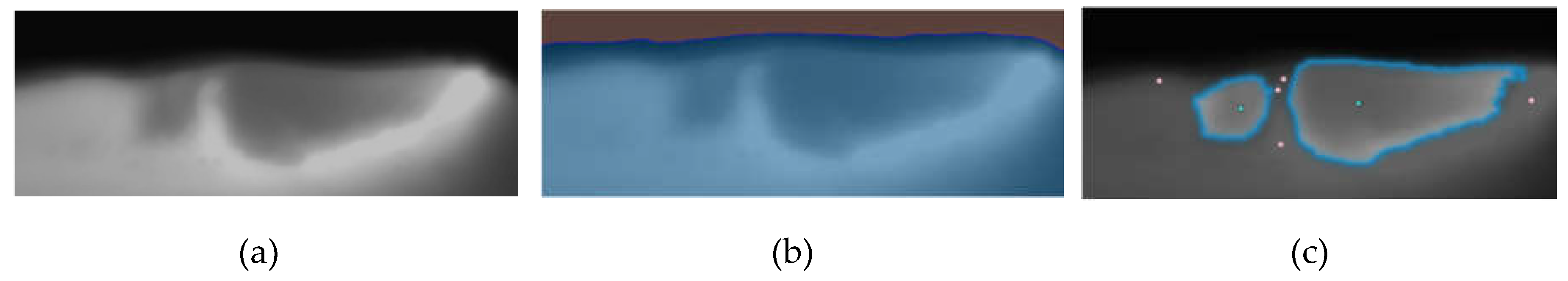
As discussed in Section4.2, the detachment-based SOTA involves using image segmentation to determine when the melt pool (MP) divides into separate volumes. Image segmentation has garnered significant attention in additive manufacturing (AM) research, leading to various successful models tailored to specific AM-related segmentation problems [31]. On the contrary, the Segment Anything Model (SAM) [30], developed by Meta, stands out due to its zero-shot learning capabilities, which allow it to operate across new datasets without further training or finetuning.
Zero-shot learning is a valuable attribute as it eliminates the need for manually annotated datasets, which is a major time-consuming and labor-intensive step in developing Deep learning models. This attribute aligns with the simplicity offered by the VIMPS tool. However, our empirical analysis, illustrated in Figure 14, demonstrates that SAM struggles with correct segmentation without human guidance (i.e., SAM “Everything” prompting). This limitation underscores a critical limitation of zero-shot learning: while promising, it does not universally guarantee effective performance across all data sets [32]. The discrepancy between the images used in initial training and those in application settings can be substantial, often necessitating the use of transfer learning techniques to bridge this gap [33,34].
Figure 14.
(a) the MP infrared image during detachment mode, the same one as in Figure 10(a). (b-i) are the SAM model segmentation results. (b) the zero-shot segmentation results without human aid, (c) the results with human aid that lead to correct segmentation, and (d-f) are the intermediate steps between (b) and (c). Interested readers can reproduce this experiment by downloading Figure(a) from the supplementary material and testing the SAM demo on the following link [35]. (b) can be obtained using the automatic “Everything” prompting, but (c-f) needs more sophisticated prompting with interactive points using the manual “Hover and Click.”.

| * | When the context is clear, the time index (t) is dropped from API(t) and PI(x,y,t) to avoid cluttered notation. But it should be clear that each of API, APIRV, APRIVM, APRIVxM and PI varies over time. |
References
- Z. Liu, B. He, T. Lyu, and Y. Zou, “A Review on Additive Manufacturing of Titanium Alloys for Aerospace Applications: Directed Energy Deposition and Beyond Ti-6Al-4V,” JOM, vol. 73, no. 6, pp. 1804–1818, Jun. 2021. [CrossRef]
- H. Chen, Z. Liu, X. Cheng, and Y. Zou, “Laser deposition of graded γ-TiAl/Ti2AlNb alloys: Microstructure and nanomechanical characterization of the transition zone,” J. Alloys Compd., vol. 875, p. 159946, Sep. 2021. [CrossRef]
- J. Ye, A. Bab-hadiashar, N. Alam, and I. Cole, “A review of the parameter-signature-quality correlations through in situ sensing in laser metal additive manufacturing,” Int. J. Adv. Manuf. Technol., vol. 124, no. 5–6, pp. 1401–1427, 2023. [CrossRef]
- T. Yu, L. Chen, Z. Liu, and P. Xu, “Research on the temperature control strategy of thin-wall parts fabricated by laser direct metal deposition,” Int. J. Adv. Manuf. Technol., vol. 122, no. 2, pp. 669–684, Sep. 2022. [CrossRef]
- Z. Mianji, A. Kholopov, I. Binkov, and K. Klimochkin, “Experimental and Numerical Study of Heat Transfer in Thin-Walled Structures Built by Direct Metal Deposition and Geometry Improvement via Laser Power Modulation,” Lasers Manuf. Mater. Process., vol. 10, no. 3, pp. 353–372, Sep. 2023. [CrossRef]
- D. Svetlizky et al., “Directed energy deposition (DED) additive manufacturing: Physical characteristics, defects, challenges and applications,” Mater. Today, vol. 49, pp. 271–295, Oct. 2021. [CrossRef]
- Z. jue Tang et al., “A review on in situ monitoring technology for directed energy deposition of metals,” Int. J. Adv. Manuf. Technol., vol. 108, no. 11–12, pp. 3437–3463, 2020. [CrossRef]
- Adebayo, J. Mehnen, and X. Tonnellier, “Limiting Travel Speed in Additive Layer Manufacturing,” 2013. [Online]. Available: https://api.semanticscholar.org/CorpusID:54218509.
- G. Turichin, E. Zemlyakov, O. Klimova, and K. Babkin, “Hydrodynamic instability in high-speed direct laser deposition for additive manufacturing,” Phys. Procedia, vol. 83, pp. 674–683, 2016. [CrossRef]
- T. C. Nguyen, D. C. Weckman, D. A. Johnson, and H. W. Kerr, “The humping phenomenon during high speed gas metal arc welding,” Sci. Technol. Weld. Join., vol. 10, no. 4, pp. 447–459, 2005. [CrossRef]
- E. Soderstrom and P. Mendez, “Humping mechanisms present in high speed welding,” Sci. Technol. Weld. Join., vol. 11, no. 5, pp. 572–579, 2006. [CrossRef]
- M. Zhang, T. Liu, R. Hu, Z. Mu, S. Chen, and G. Chen, “Understanding root humping in high-power laser welding of stainless steels: A combination approach,” Int. J. Adv. Manuf. Technol., vol. 106, no. 11–12, pp. 5353–5364, 2020. [CrossRef]
- P. Yinglei and S. Jiguo, “Understanding humping formation based on keyhole and molten pool behaviour during high speed laser welding of thin sheets,” Eng. Res. Express, vol. 2, no. 2, p. 025031, Jun. 2020. [CrossRef]
- Y. Ai et al., “Investigation of the humping formation in the high power and high speed laser welding,” Opt. Lasers Eng., vol. 107, no. May 2017, pp. 102–111, 2018. [CrossRef]
- Gullipalli, N. Thawari, and T. V. K. Gupta, “Humping defects in laser based direct metal deposition,” Mater. Today Proc., 2023. [CrossRef]
- J. Shi, F. Li, S. Chen, Y. Zhao, and H. Tian, “Effect of in-process active cooling on forming quality and efficiency of tandem GMAW–based additive manufacturing,” Int. J. Adv. Manuf. Technol., vol. 101, no. 5–8, pp. 1349–1356, 2019. [CrossRef]
- F. Montevecchi, G. Venturini, N. Grossi, A. Scippa, and G. Campatelli, “Heat accumulation prevention in Wire-Arc-Additive-Manufacturing using air jet impingement,” Manuf. Lett., vol. 17, pp. 14–18, 2018. [CrossRef]
- F. Montevecchi, G. Venturini, N. Grossi, A. Scippa, and G. Campatelli, “Idle time selection for wire-arc additive manufacturing: A finite element-based technique,” Addit. Manuf., vol. 21, no. January, pp. 479–486, 2018. [CrossRef]
- S. Singh, A. N. Jinoop, G. T. A. Tarun Kumar, I. A. Palani, C. P. Paul, and K. G. Prashanth, “Effect of interlayer delay on the microstructure and mechanical properties of wire arc additive manufactured wall structures,” Materials (Basel)., vol. 14, no. 15, 2021. [CrossRef]
- Turgut, U. Gürol, and R. Onler, “Effect of interlayer dwell time on output quality in wire arc additive manufacturing of low carbon low alloy steel components,” Int. J. Adv. Manuf. Technol., vol. 126, no. 11–12, pp. 5277–5288, 2023. [CrossRef]
- F. Dababneh and H. Taheri, “Investigation of the influence of process interruption on mechanical properties of metal additive manufacturing parts,” CIRP J. Manuf. Sci. Technol., vol. 38, pp. 706–716, 2022. [CrossRef]
- R. Denlinger, J. C. Heigel, P. Michaleris, and T. A. Palmer, “Effect of inter-layer dwell time on distortion and residual stress in additive manufacturing of titanium and nickel alloys,” J. Mater. Process. Technol., vol. 215, pp. 123–131, 2015. [CrossRef]
- S. C. A. Alfaro, J. A. R. Vargas, G. C. De Carvalho, and G. G. De Souza, “Characterization of ‘humping’ in the GTA welding process using infrared images,” J. Mater. Process. Technol., vol. 223, pp. 216–224, 2015. [CrossRef]
- B. Xue, B. Chang, and D. Du, “A vision based method for humping detection in high-speed laser welding,” J. Phys. Conf. Ser., vol. 1983, no. 1, p. 012074, Jul. 2021. [CrossRef]
- J. Lu, Z. Zhao, J. Han, and L. Bai, “Hump weld bead monitoring based on transient temperature field of molten pool,” Optik (Stuttg)., vol. 208, no. October 2019, p. 164031, Apr. 2020. [CrossRef]
- S. J. Altenburg, A. Straße, A. Gumenyuk, and C. Maierhofer, “In-situ monitoring of a laser metal deposition (LMD) process: Comparison of MWIR, SWIR and high-speed NIR thermography,” Quant. Infrared Thermogr. J., vol. 19, no. 2, pp. 97–114, Mar. 2022. [CrossRef]
- R. A. Felice and D. A. Nash, “Pyrometry of materials with changing, spectrally-dependent emissivity-Solid and liquid metals,” AIP Conf. Proc., vol. 1552 8, pp. 734–739, 2013. [CrossRef]
- “Emissivity Values for Metals.” https://www.flukeprocessinstruments.com/en-us/service-and-support/knowledge-center/infrared-technology/emissivity-metals (accessed Oct. 04, 2024).
- C. Slater, K. Hechu, C. Davis, and S. Sridhar, “Characterisation of the solidification of a molten steel surface using infrared thermography,” Metals (Basel)., vol. 9, no. 2, pp. 1–9, 2019. [CrossRef]
- Kirillov et al., “Segment Anything,” 2023, [Online]. Available: https://ai.facebook.com/research/publications/segment-anything/.
- J. Zhang et al., “Image Segmentation for Defect Analysis in Laser Powder Bed Fusion : Deep Data Mining of X - Ray Photography from Recent Literature,” Integr. Mater. Manuf. Innov., vol. 11, no. 3, pp. 418–432, 2022. [CrossRef]
- B. Blumenstiel, J. Jakubik, H. Kühne, and M. Vössing, “What a MESS: Multi-Domain Evaluation of Zero-Shot Semantic Segmentation,” Jun. 2023, Accessed: Apr. 14, 2024. [Online]. Available: https://arxiv.org/abs/2306.15521v3.
- M. A. Hassan, R. ElMallah, and C. G. Lee, “Approximate and Memorize (A&M): Settling opposing views in replay-based continuous unsupervised domain adaptation,” Knowledge-Based Syst., vol. 293, no. December 2023, p. 111653, 2024. [CrossRef]
- M. Abubakr, B. Akoush, A. Khalil, and M. A. Hassan, “Unleashing deep neural network full potential for solar radiation forecasting in a new geographic location with historical data scarcity: A transfer learning approach,” Eur. Phys. J. Plus, vol. 137, no. 4, 2022. [CrossRef]
- “Segment Anything | Meta AI.” https://segment-anything.com/ (accessed Apr. 14, 2024).
Figure 1.
(a) real image of severe humping redrawn from [8] showing the crests and valleys forming the wavy structure. Each column (i.e., from b to f) shows different melt pool modes with humping’s severity increasing from b to f. Within each column, time progresses from top to bottom.
Figure 1.
(a) real image of severe humping redrawn from [8] showing the crests and valleys forming the wavy structure. Each column (i.e., from b to f) shows different melt pool modes with humping’s severity increasing from b to f. Within each column, time progresses from top to bottom.
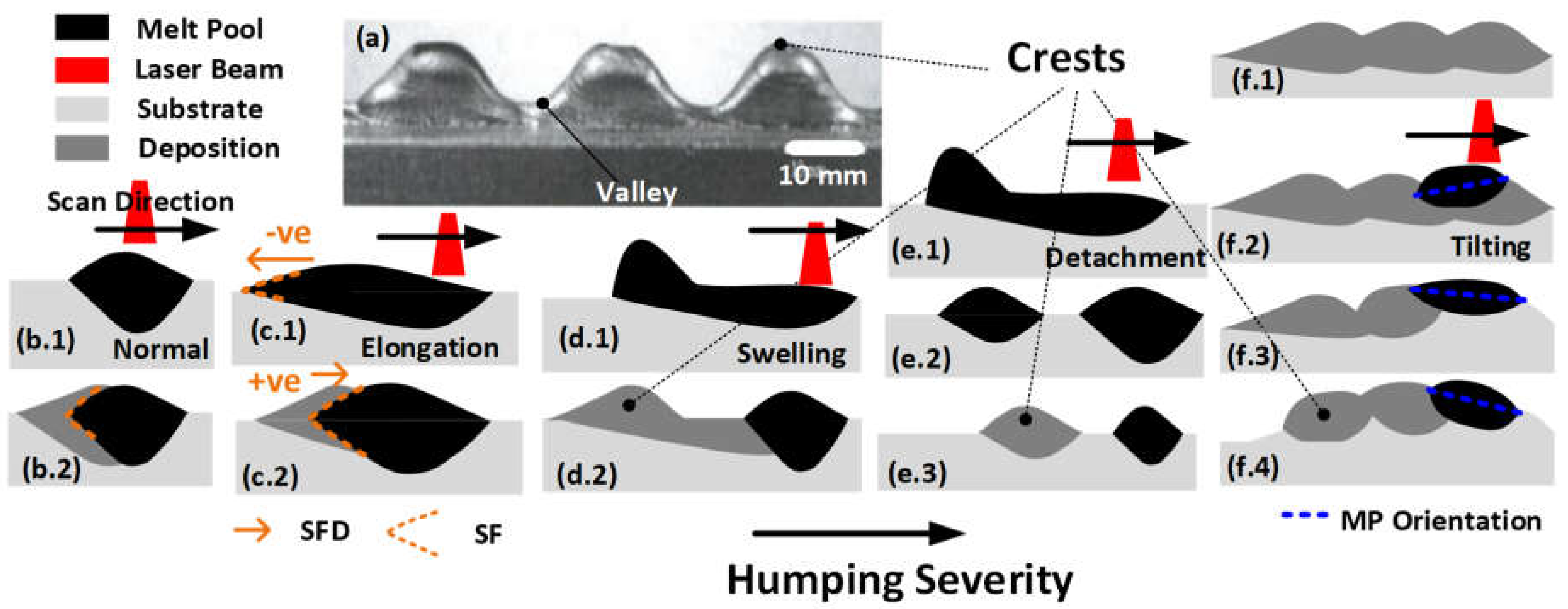
Figure 2.
Laser profile used.
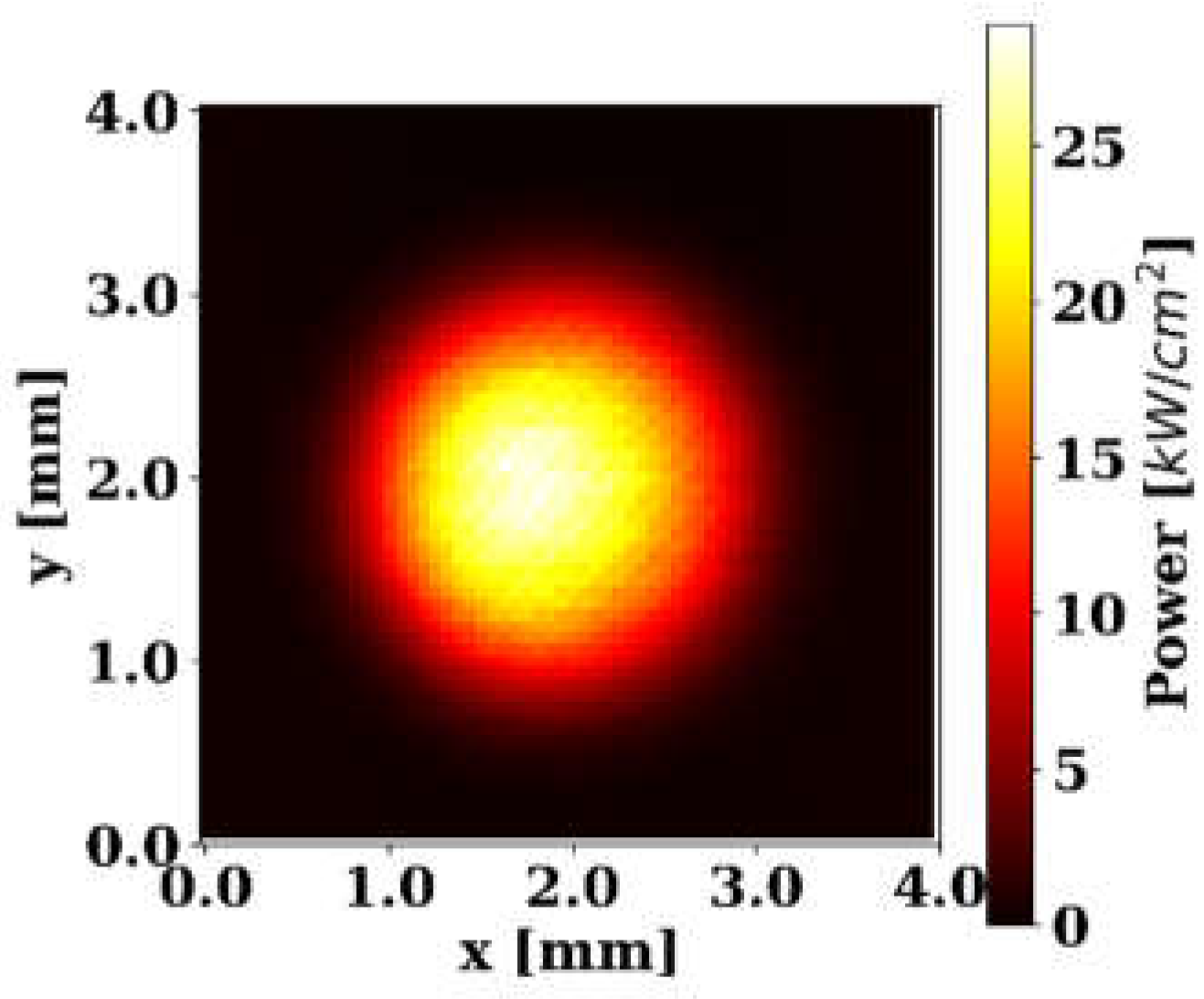
Figure 3.
(a) Schematic (b) actual view of the experimental setup.
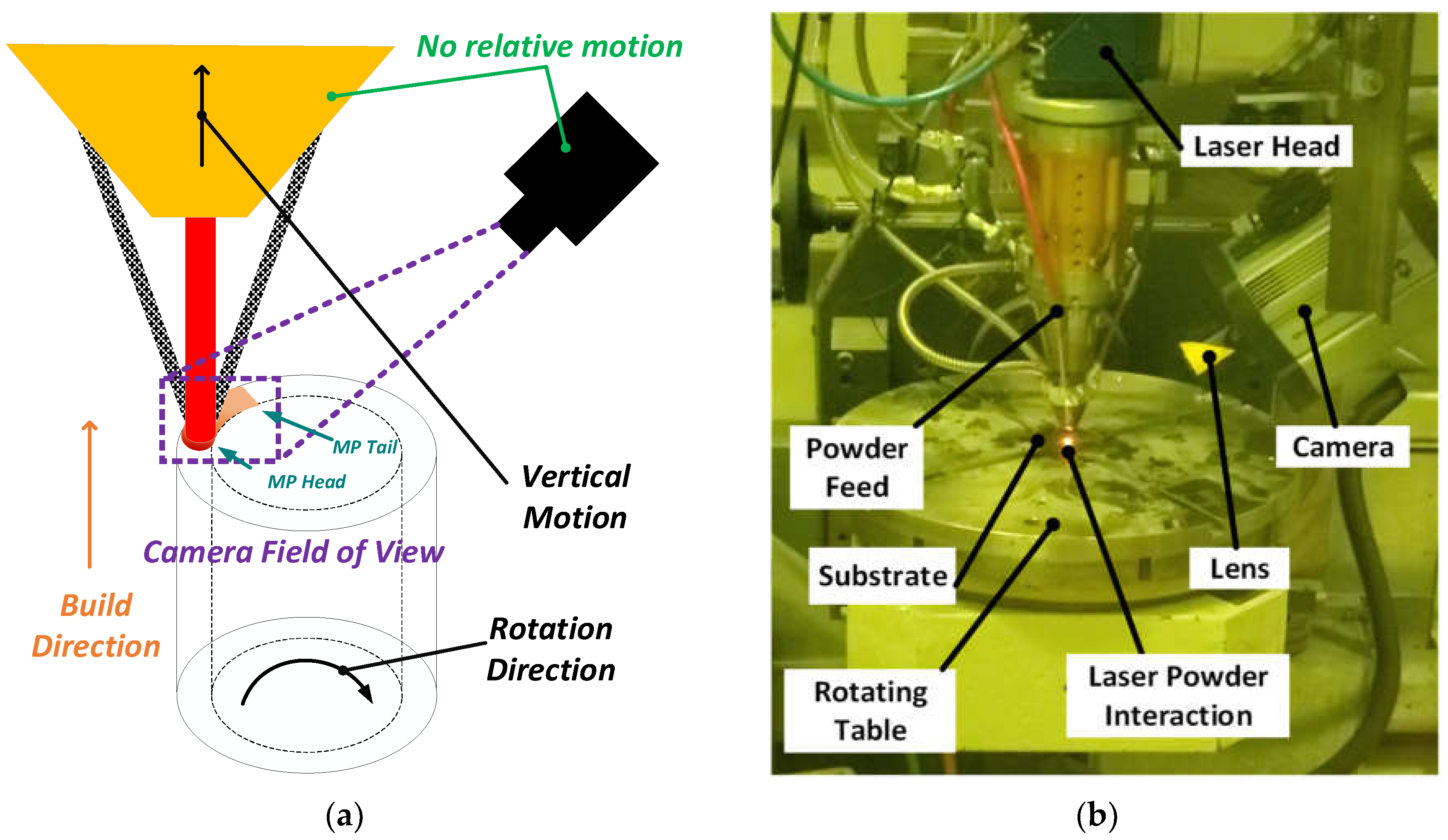
Figure 4.
The melt pool and the approximate contour of the heat-affected zone (HAZ).
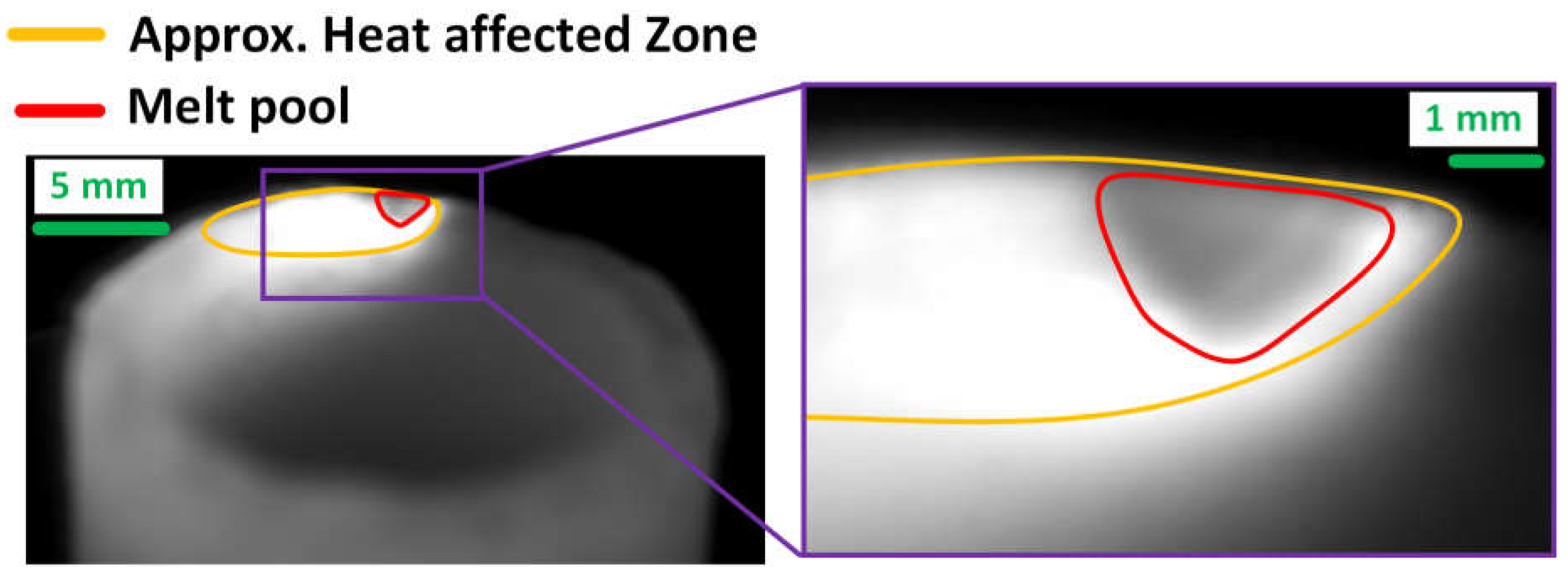
Figure 5.
The progression of melt pool solidification after the laser was turned off. Note t = 303.75 sec corresponds to the moment at which the laser was turned off.
Figure 5.
The progression of melt pool solidification after the laser was turned off. Note t = 303.75 sec corresponds to the moment at which the laser was turned off.
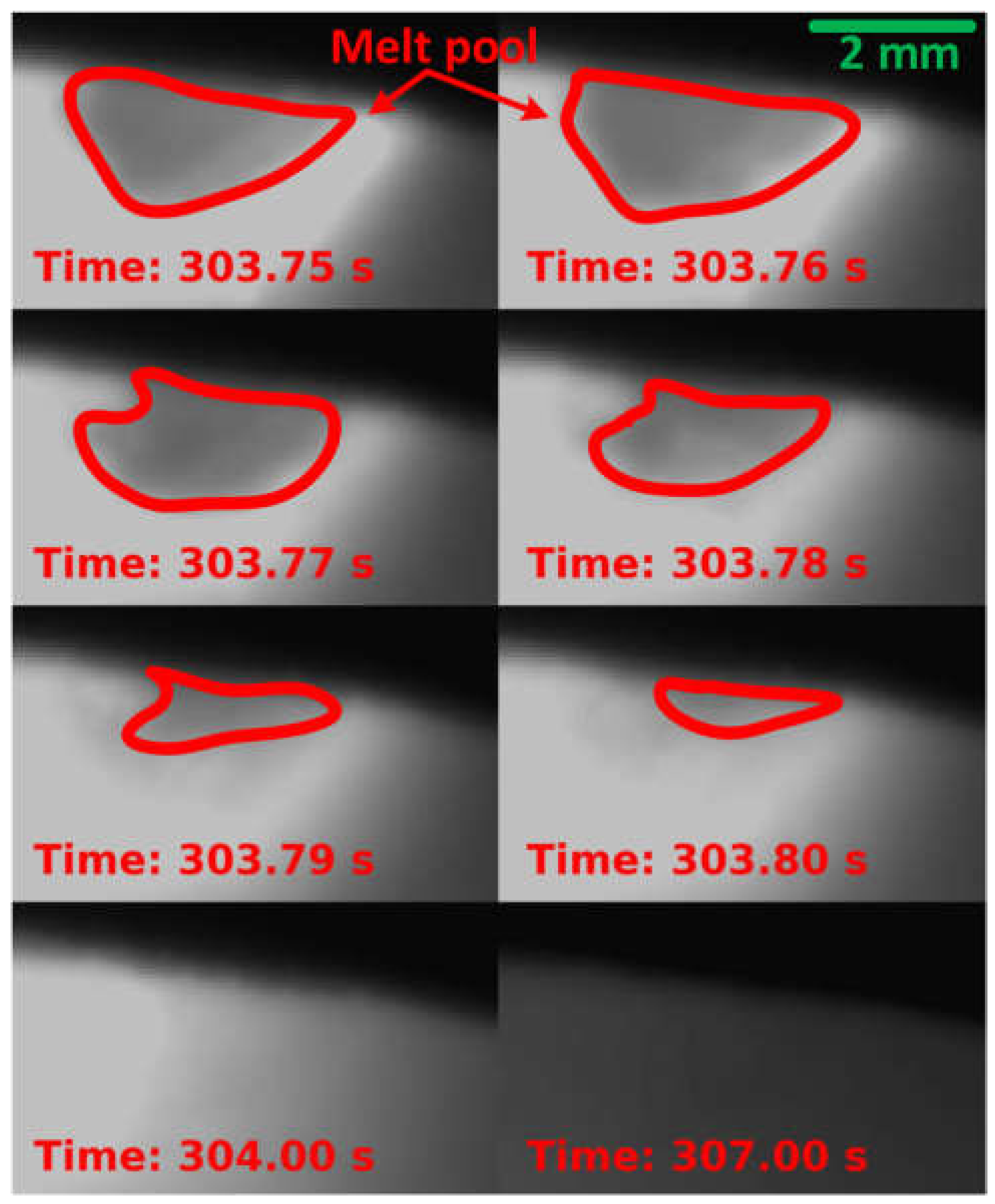
Figure 6.
(d) API variations during the accumulation (a→b) and solidification (b→c) through one elongation mode cycle.
Figure 6.
(d) API variations during the accumulation (a→b) and solidification (b→c) through one elongation mode cycle.
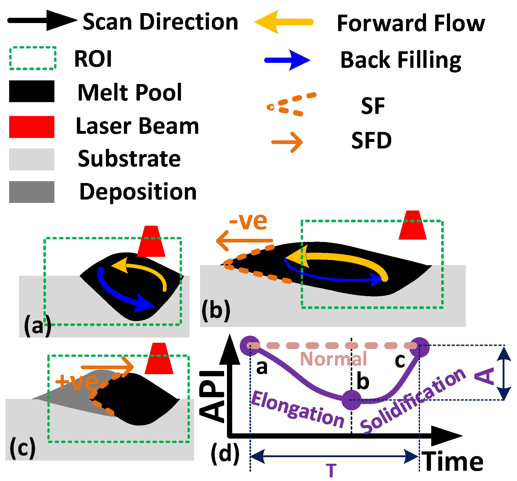
Figure 7.
As printed parts, (a & d) Test-1. (b & e) Test-2, and (c & f) Test-3. (d, e & f top-view with an elevation map (i.e., topography). Yellow regions are higher than blue regions by 1 mm, as shown in the scale in (f). Note that the variations in (e) and (f) are mainly due to the helical printing path, while in (d), the variations are dominated by the humping-induced crests.
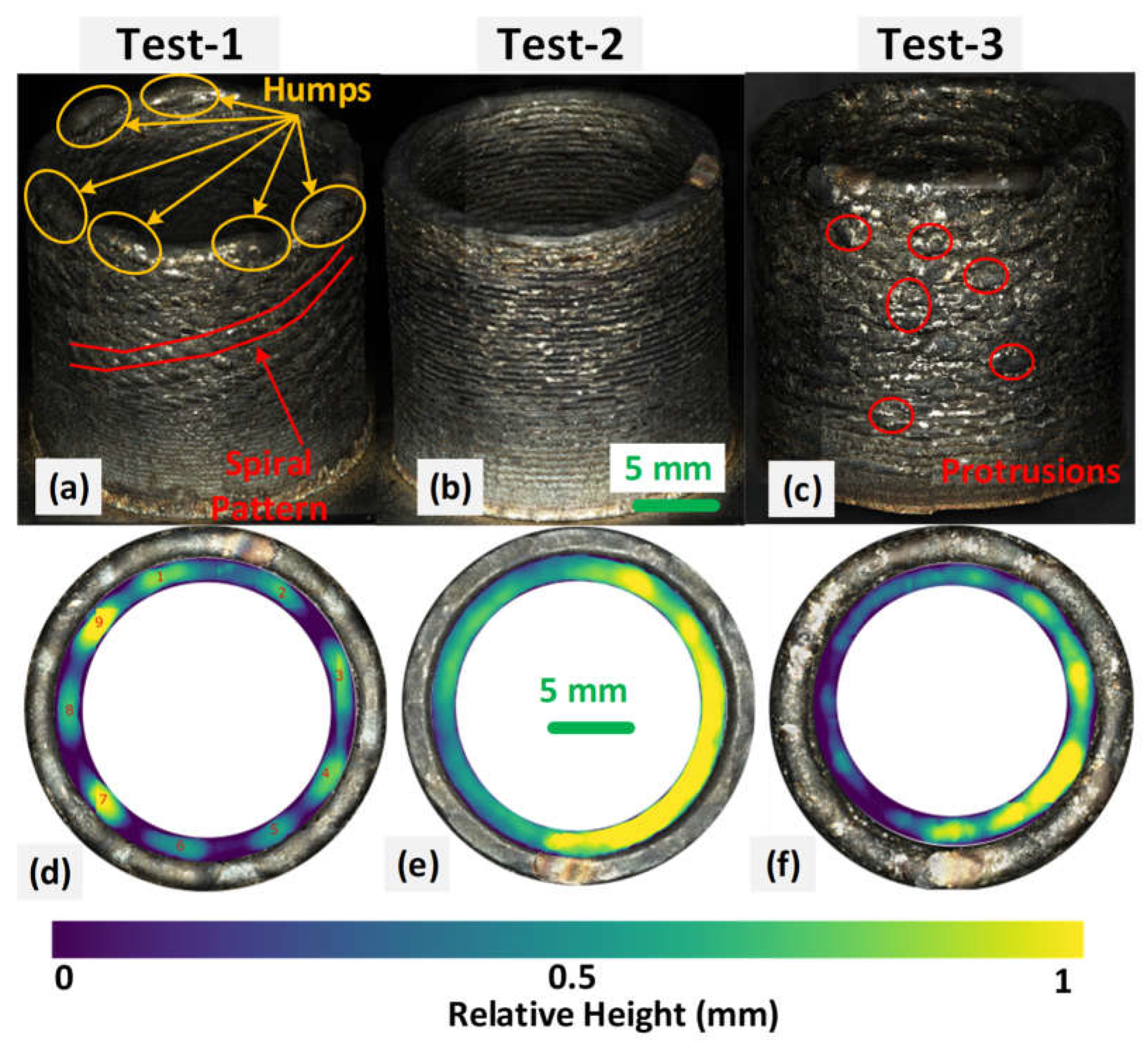
Figure 8.
The VIMPS variation over for different prints.
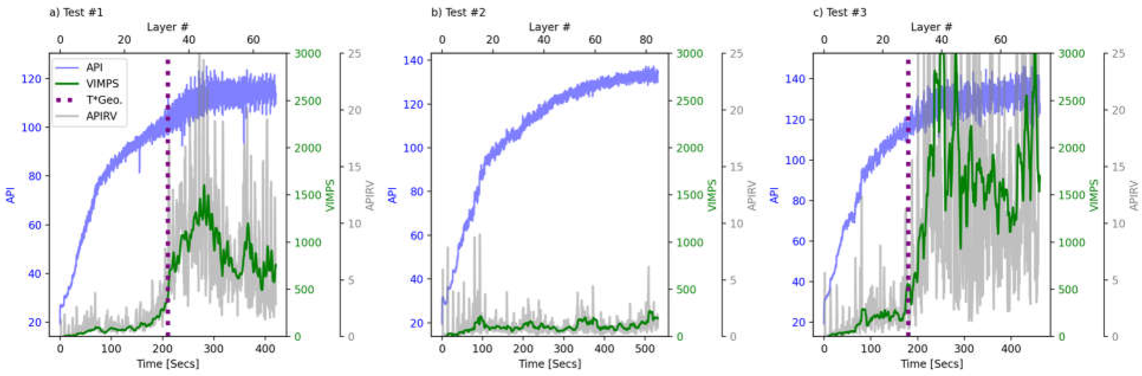
Figure 9.
(a) VIMPS overlayed over the as-printed part surface topography, (b) Side view of the as-printed part highlighting the scanned whose surface topography is shown in subfigure (a) in the same Figure.
Figure 9.
(a) VIMPS overlayed over the as-printed part surface topography, (b) Side view of the as-printed part highlighting the scanned whose surface topography is shown in subfigure (a) in the same Figure.
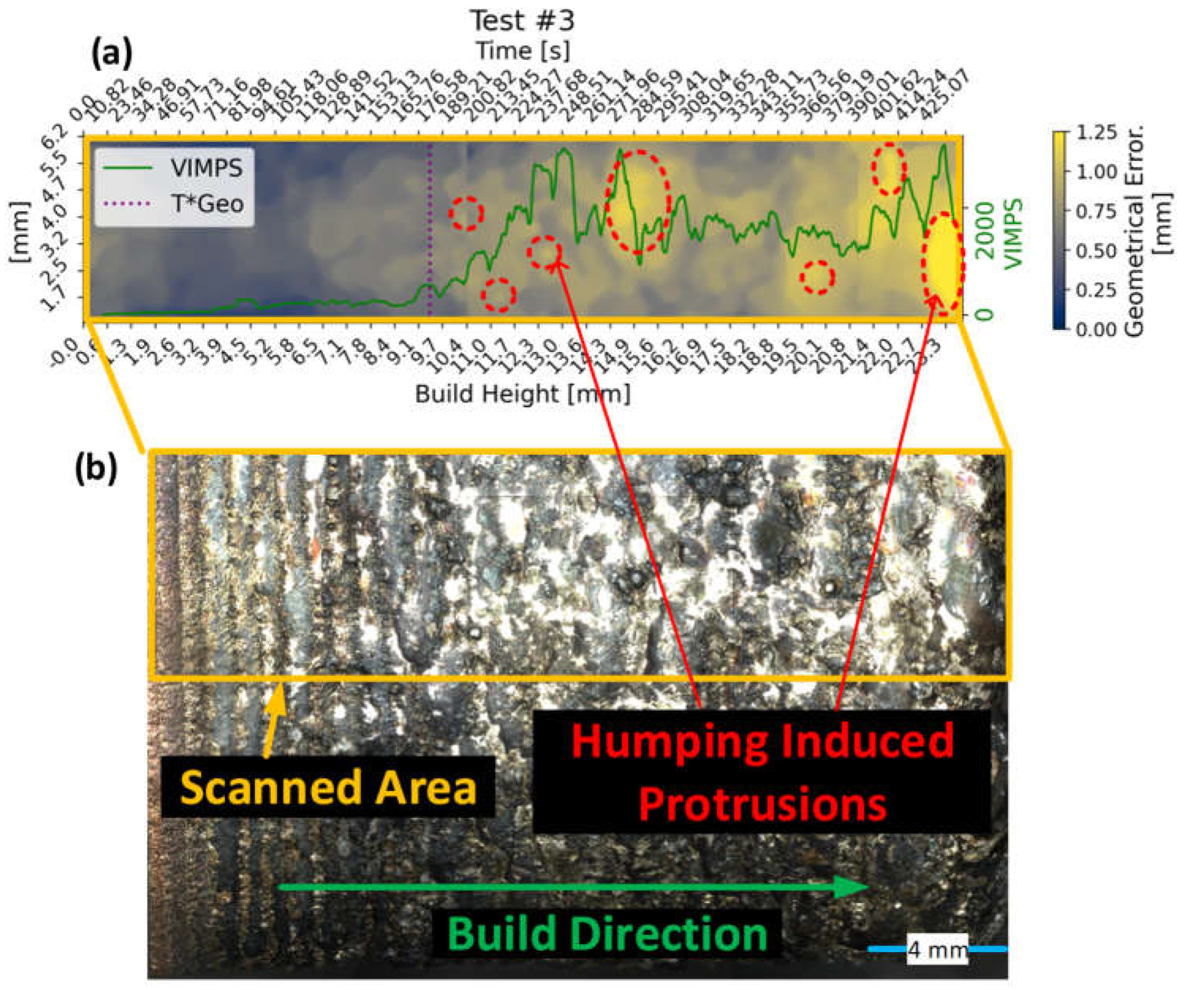
Figure 10.
Manually annotated melt pool at the detachment mode. (a-b) From Test #1 and (c-d) from Test #3. (a,c) show the first instances of the detachment mode in the corresponding test, and (b,d) shows the second instance.
Figure 10.
Manually annotated melt pool at the detachment mode. (a-b) From Test #1 and (c-d) from Test #3. (a,c) show the first instances of the detachment mode in the corresponding test, and (b,d) shows the second instance.
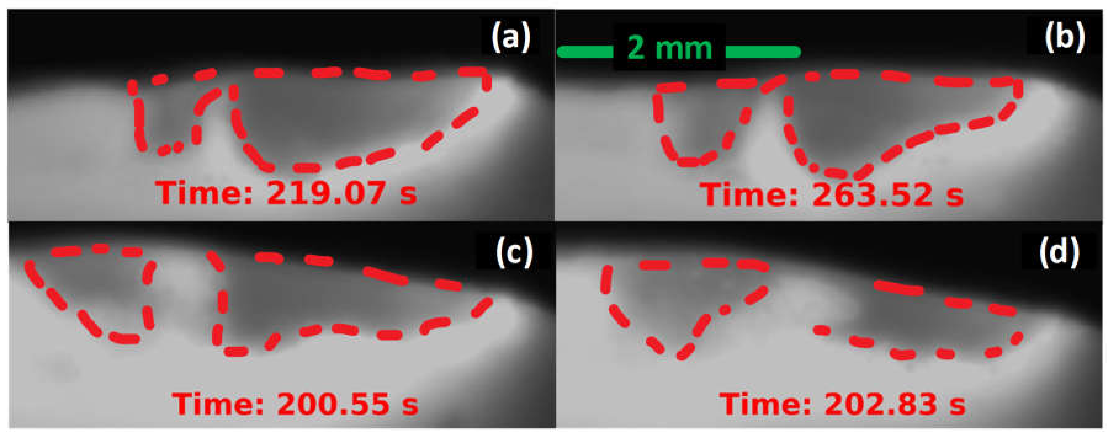
Figure 11.
(a) API during tilting in Test#1 (i.e., layer-32 to layer-44) and (b) the FFT analysis of the API- APIRM.
Figure 11.
(a) API during tilting in Test#1 (i.e., layer-32 to layer-44) and (b) the FFT analysis of the API- APIRM.
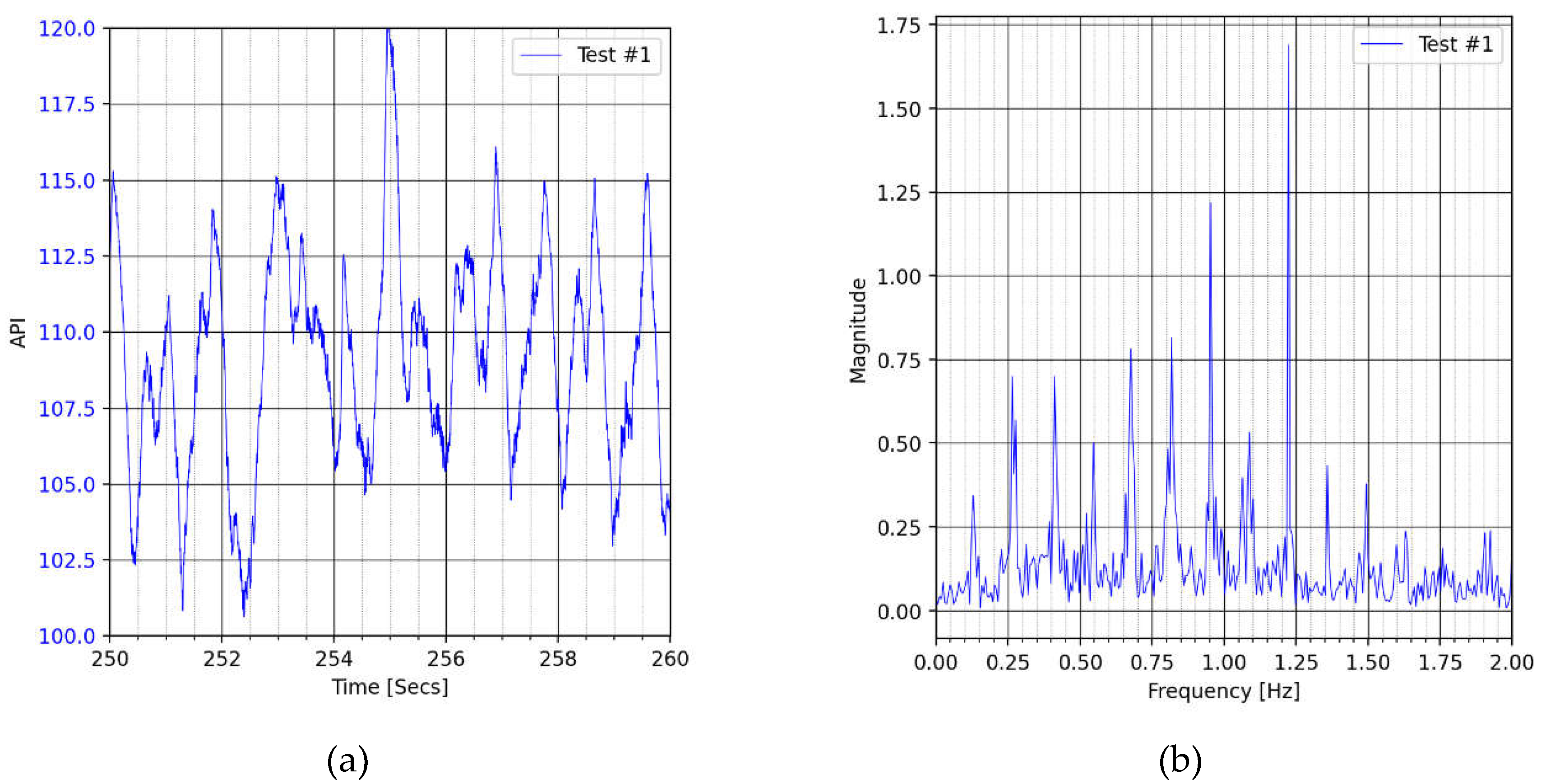
Figure 12.
micro-protrusion during Test #2.
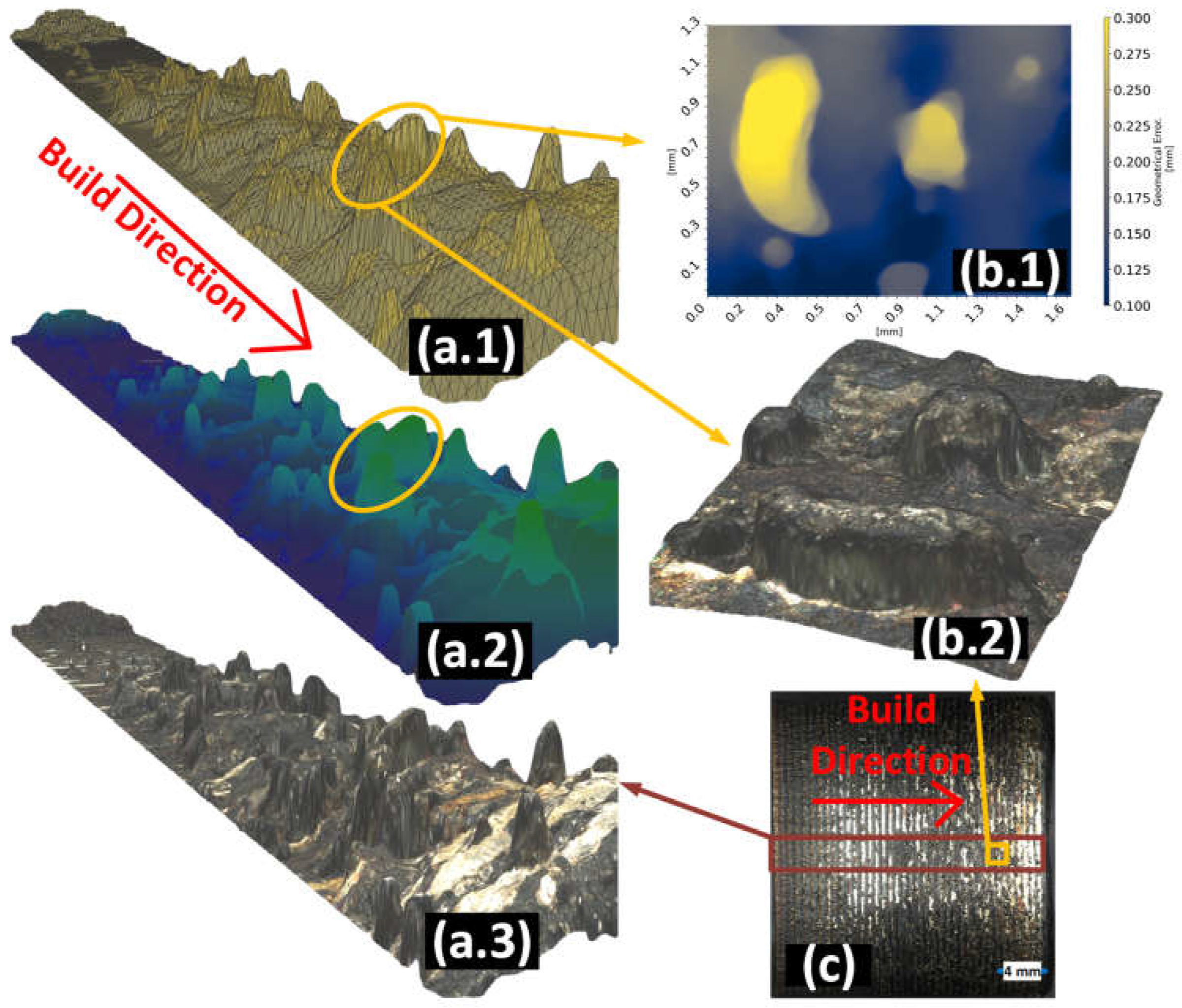
Figure 13.
(a) Early (b) late infrared images from test#1 and (c) late test#2. The accumulation step begins in (x.1) and ends in (x.2), and the solidification step starts in (x.2) and ends in (x.3). Subplots x.4 show the pixel intensity increase during the solidification (i.e., the pixel-wise difference between (x.3) and (x.2). Subplots x.5 show the API and VIMPS variation during the elongation cycle.
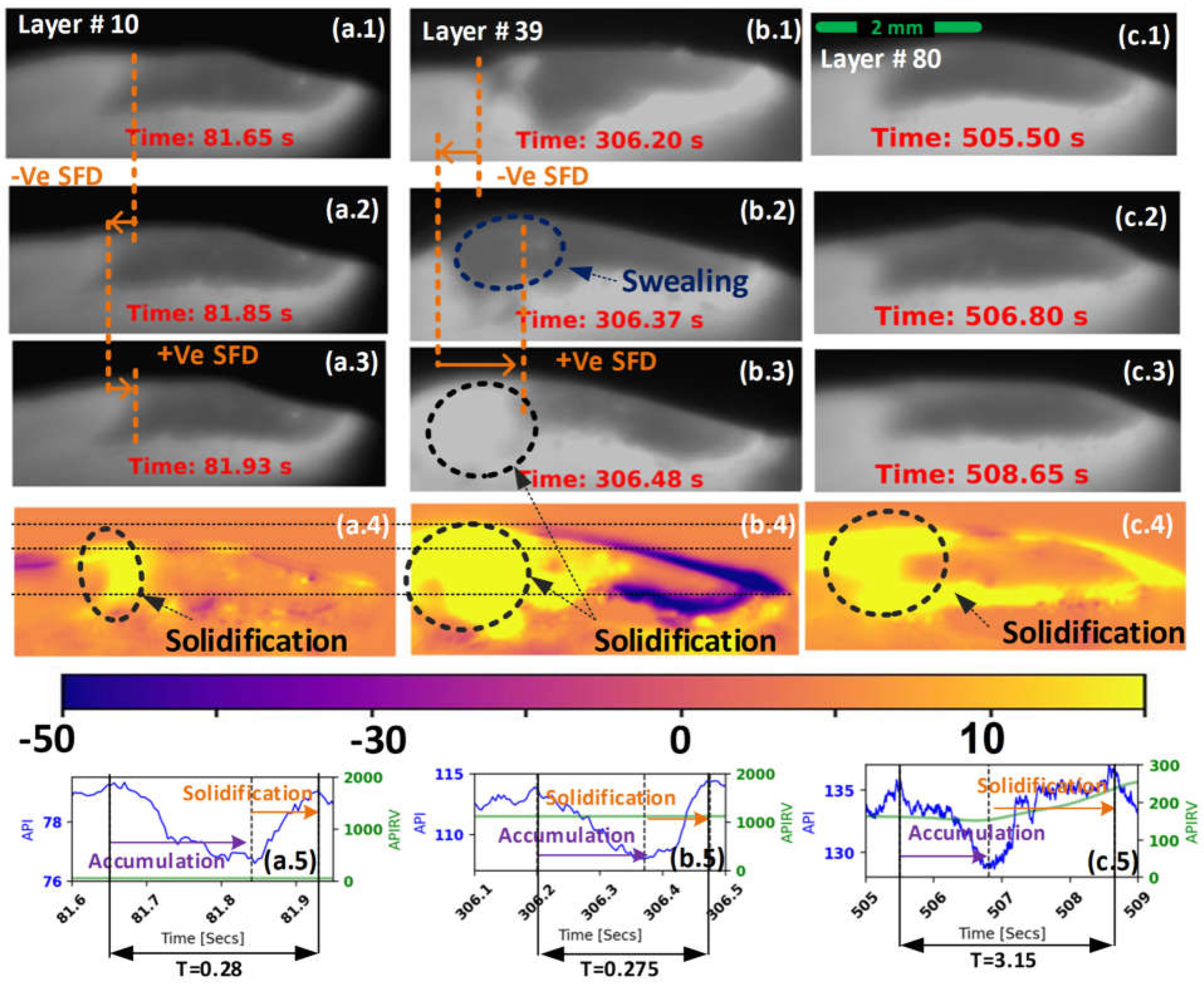

Table 1.
Experimental test matrix.
| Test No. | P (W) | V (mm/min) |
| 1 | 650 | 600 |
| 2 | 650 | 360 |
| 3 | 850 | 360 |
Table 2.
Variation of different physical quantities during the elongation mode.
| MP size | SFD | API | |
| Accumulation in Figure 1c.1. | Increasing | Negative | Decreasing |
| Solidification in Figure 1c.2. | Decreasing | Positive | Increasing |
Table 3.
Pseudocode for Physics-Based Indicator methodology.
| Line | Pseudo Code |
| 1 | Define Region of Interest (ROI) |
| 2 | do: |
| 3 | Calculate Average Pixel Intensity (API) as per Equation 1 |
| 4 | Calculate API’s Rolling Mean (APIRM) as per Equation 2 |
| 5 | Calculate API’s Rolling Variance (APIRV) as per Equation 3 |
| 6 | Calculate APIRVxM as per Equation 4 |
| 7 | Calculate (VIMPS) as per Equation 5 |
| 8 | End For |
Table 4.
Comparative analysis of humping detection methods; all values are in seconds.
| Metric | VIMPS | SOTA’s Theoretical Upper bound |
||
| Test # | 1 | 3 | 1 | 3 |
| Detection Time | 200 | 170 | 219 | 200 |
| T*Geo Time | 210 | 180 | 210 | 180 |
| Detection Lead | 10 | 10 | -9 | -20 |
| Consistency | High | Low | ||
| Complexity | Low | High | ||
| Principle | Spatiotemporal | Spatial | ||
| Mode | Elongation | Detachment | ||
♦ Note that this is an upperbound for the SOTA performance as detachments in this figure were detected by human annotator. In reality, lower performance is expected due to error is expected depending on the sophisticated on the segmentation approach used.
Disclaimer/Publisher’s Note: The statements, opinions and data contained in all publications are solely those of the individual author(s) and contributor(s) and not of MDPI and/or the editor(s). MDPI and/or the editor(s) disclaim responsibility for any injury to people or property resulting from any ideas, methods, instructions or products referred to in the content. |
© 2024 by the authors. Licensee MDPI, Basel, Switzerland. This article is an open access article distributed under the terms and conditions of the Creative Commons Attribution (CC BY) license (http://creativecommons.org/licenses/by/4.0/).
Copyright: This open access article is published under a Creative Commons CC BY 4.0 license, which permit the free download, distribution, and reuse, provided that the author and preprint are cited in any reuse.


