1. Introduction
The current level of development in communication, information, and sensor technologies enables the automation of monitoring and managing complex systems that previously required expert intervention. This automation enhances scalability and responsiveness [
1,
2,
3].
Scalability, real-time monitoring, and control are increasingly feasible and essential for transport systems, leading to improved safety and efficiency in their operations [
4]. Intelligent Transport Systems (ITS) utilizing vehicle-to-everything (V2X) technology [
5] meet the demands of modern transport systems [
6,
7,
8] by continuously collecting data on road traffic through various sensors [
4]. The collected and systematized data, which represents the context of traffic situations, is crucial for determining the evolving requirements of ITS functionality over time [
9]. Context data plays a vital role in analyzing sensor data, reasoning, and modeling intelligent systems, significantly impacting the effectiveness of ITS. The interaction diagram of the Physical and Virtual Transport Space (PTS, VTS) within the Metaverse Transportation System provides a comprehensive representation of the context of the entire transport system [
10].
The VTS supports computational experiments with feedback optimization relative to the real PTS [
10], which connects the operation of many systems at a high level and controls the generation of data facilitating the integration of machine learning (ML) models into ITS operations. VTS can be implemented using various approaches that consider the mobility of their elements. Macroscopic traffic simulation modeling addresses the mobility of elements within transport systems, enabling controlled generation of key traffic flow characteristics.
The Simulation Model of Traffic Flow (SMTF) generates random events representing vehicle appearances on simulated routes based on the context of traffic situations embedded in the model. Predetermined parameters and time within the simulated space define this context [
11], influencing movement scenarios, interactions, traffic density, and infrastructure behavior on the road.
Macroscopic traffic models focus on vehicle behavior and statistical characteristics. Therefore, most implementations of these models concentrate on depicting the dynamics of a specific section of the route based on available data [
12]. Various software solutions are available to simplify the construction of a macroscopic model, with one notable example being the SUMO (Simulation of Urban Mobility) software widely utilized in research fields, particularly in traffic management and transportation communications [
13]. SUMO offers capabilities for constructing, adjusting, and modeling custom traffic flow architectures, along with supporting tools for importing network and demand models of existing route sections.
The demand model determines the frequency of selecting different routes on a specific highway section, including the starting and ending points of vehicles and their type selection. Therefore, the accuracy of this model is crucial in road simulation as it reflects the primary needs of drivers for city navigation [
14] and influences the value of the resulting SMTF.
SUMO's versatility enables the study of traffic control strategies and vehicular communication systems [
15]. The high-detailed simulation in SUMO is essential for analyzing and optimizing traffic management strategies, evaluating the impact of infrastructure modifications, and examining vehicle interactions in complex urban environments [
16]. Additionally, SUMO supports V2X technology modeling, facilitating the development and testing of interoperable automotive applications [
17].
However, a significant drawback of such models is their challenge in adapting to dynamic changes in the PTS [
18]. The accuracy of the simulated model data may differ significantly from that of real-life PTS data since the simulation's source data relies on information from the OpenStreetMap (OSM) project. Updating the OSM database can be slow and dependent on the location and activity of volunteers in the relevant region [
19].
The demand model and vehicle behavior parameters show the most significant differences from real-world traffic data in PTS. The demand model affects how traffic density is distributed over space and time, which can be monitored using data from ITS sensor systems [
20]. To address discrepancies between the outdated demand model and current traffic conditions, adjustments can be made to the spatial and temporal distribution of traffic density in the SMTF through calibration of simulation models.
Various calibration techniques can help bridge the gap between the simulated model and actual traffic conditions in FTP. These include direct calibration of the demand model [
21,
22,
23,
24,
25], calibration of the macroscopic model based on physical processes [
26,
27,
28], and the use of evolutionary algorithms to optimize calibration parameters [
29,
30,
31]. Studies suggest that relying on a single traffic flow model may not capture all relevant phenomena accurately, potentially impacting simulation accuracy [
32]. Hybrid traffic flow models, combining microscopic, mesoscopic, and macroscopic approaches [
33,
34,
35,
36,
37], offer a more comprehensive representation of traffic dynamics with varying levels of scalability.
Another way to enhance simulation accuracy is by integrating macroscopic modeling with ML techniques to improve prediction accuracy and adaptability to changing traffic conditions [
38,
39,
40]. This hybrid approach can provide greater flexibility to changing traffic patterns by combining the overall traffic flow dynamics captured by macroscopic models with ML's ability to handle dynamic changes effectively. By leveraging ML methods instead of traditional statistical approaches, traffic modeling algorithms can achieve higher accuracy and adaptability [
41].
In [
42], it is demonstrated that ML can be helpful in dynamically calibrating parameters in macroscopic traffic flow models. For instance, ML can generate a set of hyperparameters for calibration through generative adversarial simulation learning. However, a challenge arises in selecting a data source to timely calibrate the VTS to reflect changes in the PTS.
One increasingly popular method for collecting traffic flow data from specific highway sections is the use of Wireless Sensor Networks (WSN) due to their flexibility, scalability, and cost-effectiveness, as highlighted in [
43,
44,
45,
46,
47,
48]. WSNs allow data collection on parameters recorded by sensors from each vehicle connected to the communication network, providing more detailed information about the analyzed route section than analyzing traffic video streams [
49]. This richer data can help address a broader range of ITS problems through ML.
Despite the benefits of using WSNs, video recording systems, especially those based on autonomous aerial vehicles, are becoming more prevalent [
50,
51] thanks to advancements in ML methods for processing video streams [
52] and the proliferation of city cameras. This trend enables the creation of extensive and affordable systems for collecting transport network data to build and calibrate simulation models [
53,
54,
55]. Video systems allow data collection from all vehicles without specialized sensors or communication modules. On the other hand, integrating a large number of vehicles into a WSN can present challenges.
However, it is essential to note that a fixed dataset is required to address various challenges in constructing SMTF for specific route sections, conducting computational experiments, and pre-training ML models for integration into VTS [
56,
57,
58]. This dataset cannot always be directly obtained from video streams, and deploying WSNs may be hindered by the lack of vehicles equipped with transceiver systems and sensors.
In our previous work [
15], we showcased an application of ML in ITS focusing on specific traffic flow data. The approach involved generating synthetic data to train the ML algorithm within the vehicle-to-infrastructure (V2I) system, leveraging the SUMO simulation model and the Longley-Rice propagation model [
59]. The primary objective was to reduce delays in the V2I network, including minimizing network connection time. By creating a method for generating diverse motion scenarios, the algorithm's ability to generalize for antenna radiation tuning was enhanced.
The ML algorithm, trained on the synthetic dataset, exhibited a 94% accuracy in determining the optimal main lobe position crucial for establishing and sustaining a dependable connection between the V2I infrastructure and vehicles. However, when tested on real data extracted through intelligent processing of video streams from the simulated area, the accuracy dropped by over 40% compared to synthetic data. This discrepancy highlighted a significant deviation between the characteristics distribution generated by the simulation model and actual traffic flow data.
This paper proposes a solution to develop SMTFs that closely align with real-world PTS. The methodology involves a hybrid regression calibration of a macroscopic model using SUMO data, leveraging real-time video stream analysis with the ML algorithm to capture vehicle characteristics within the modeled area.
The paper is structured as follows:
Section 2 outlines how to represent PTS dynamics within a VTS and details the process for creating and calibrating the proposed SMTF.
Section 3 introduces a method for analyzing video streams and extracting relevant data.
Section 4 presents simulation results demonstrating the algorithm's performance in calibrating a macroscopic traffic model with new data from the PTS. Additionally, it showcases an experiment assessing the calibrated SUMO model's alignment with real PTS based on video stream data and connected car sensors.
2. Analysis of the Influence of the Dynamics of the PTS on the Operation of the VTS and the Structure of the Proposed ITS
The processes within the transportation flow can vary depending on the specific focus of the study. When examining traffic flow on a specific section of the road, several overarching factors come into play. These include the overall road infrastructure both within and outside the section being studied [
60,
61,
62], as well as temporary factors that can be cyclic, like changes in time of day and seasons [
23,
63,
64], or random, such as variations in weather conditions [
65].
These global and temporal factors also fluctuate and influence traffic flow characteristics to different extents, which can make simulation modeling quite complex [
23,
64]. To simplify this complexity, a limited set of traffic flow parameters is required to develop SMTF and assess the dynamics of each parameter.
In the context of the previous work [
15], the selected parameters for addressing the vehicle tracking issue were sensor data that reflect the internal attributes of vehicles while they are in motion. Since these vehicle sensor parameters exhibit a spatial and temporal distribution that aligns with the traffic demand model, analyzing this data offers valuable preliminary insights into the modeled area. Additionally, it supplements Global Navigation Satellite System (GNSS) data in cases where GNSS data is inaccurate or unavailable due to interference or a lack of visible satellites [
66,
67].
The data used to train the developed algorithm for tracking vehicle movement included the time mark when a request was sent to connect to an intelligent infrastructure facility, the vehicle's speed, and its rotation angle relative to geographic north.
As observed in the VTS analysis from [
15], these parameters' dynamics experience temporary fluctuations, leading to deviations in the demand model. These deviations are evident in changes in the frequency of vehicles on various sections of the route over time. During the analysis, a deviation in the demand model was specifically noted, resulting in fluctuations in the frequency of vehicle presence along different segments of the route overall and over specific time intervals.
We divided the simulated area into sectors using the Geohash method [
68] of GNSS coordinate space encoding with a code sequence length of 8. Each sector measured 38.2 m by 19.1 m. This level of detail is considered optimal for Vehicle-to-Infrastructure (V2I) technology, which typically has an average range of 600 m [
5]. The sector sizes were chosen to match the dimensions of route elements like intersections and turns.
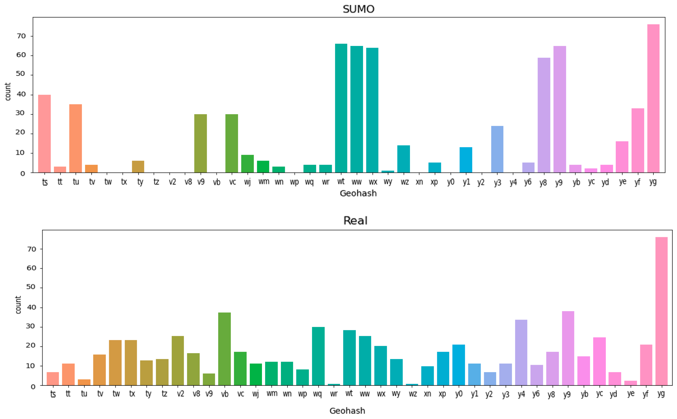
Our analysis of the positioning algorithm involved comparing vehicle coordinates obtained from SUMO with results from video stream analysis. The differences in sector boundary crossing frequencies between the SUMO model and video stream processing data are shown in
Figure 1.
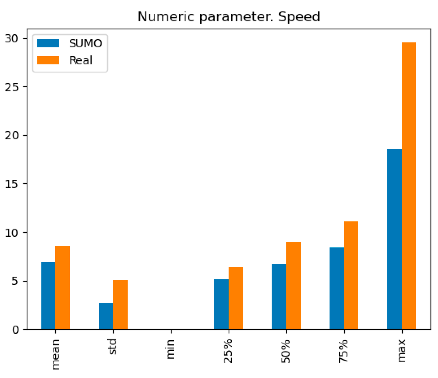
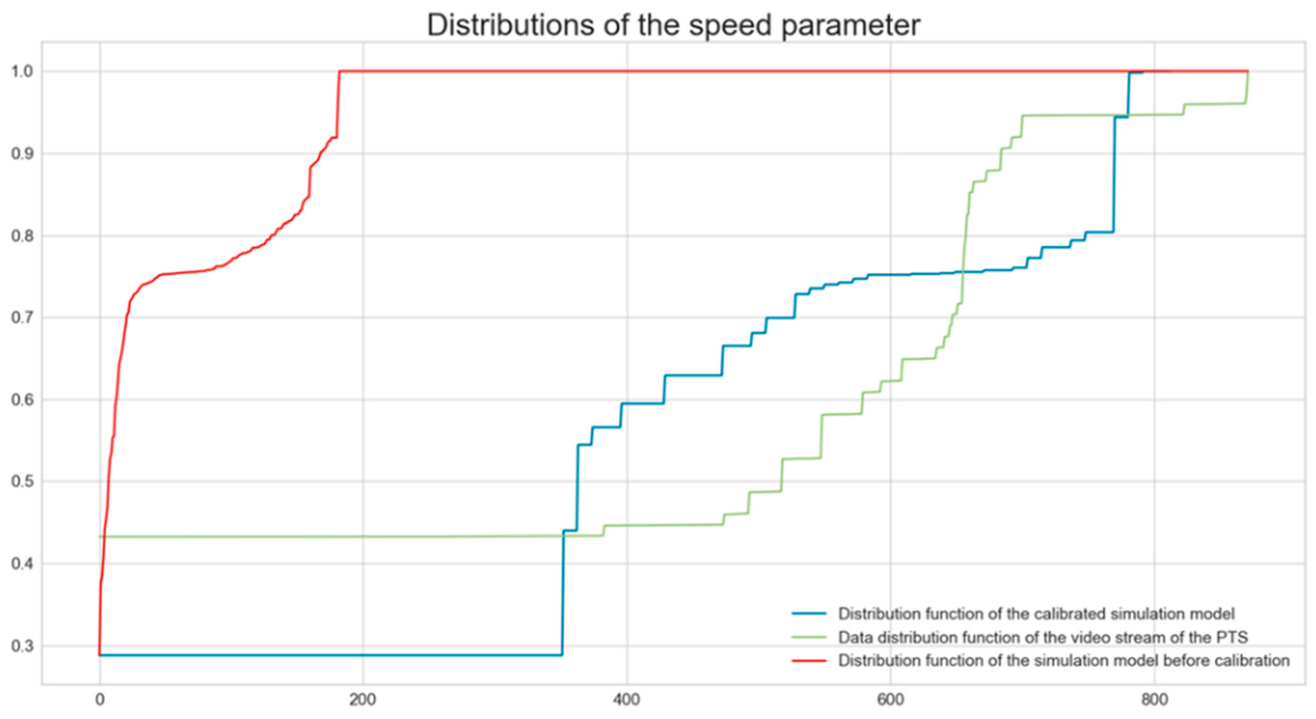
Changes in the demand model led to variations in the distribution characteristics of the generated traffic flow parameters.
Figure 2 illustrates the deviation in time-averaged vehicle speed values generated compared to data from the video stream.
To address deviations in the SMTF from real-world PTS, we developed a new ML-based simulation model. Initially, SUMO was used to train the model, which was then fine-tuned using data from PTS.
2.1. Dynamics of Traffic Flow as Data Drift
In the context of the VTS intelligent algorithms, changes in the probability distribution of data from the PTS can be seen as data drift [
69]. This drift can be categorized into three types when PTS is viewed through a statistical model with input data X and output processing data Y. The first type (or drift of the first kind) is the drift of input data X, which reflects changes in traffic flow density due to daily, weekly, or seasonal cycles [
70] and other time-related factors. The second type (the drift of the second kind) is the drift of output data Y, which could manifest as a shift in the simulation model's trace graph relative to the PTS due to external factors. The third type (the drift of the third kind) is simultaneous changes in both input and output data X and Y, indicating the combined influence of global and local factors.
Data drift from PTS dynamics directly impacts the accuracy of simulation modeling, especially when using ML models, as the distribution of input data used for analysis and training becomes outdated [
10]. Therefore, calibrating the SMTF is essential to adapt to PTS data drift.
The data calibration process includes four stages [
69]:
Data extraction: Collecting data fragments from streams to create a current sample of the studied parameter.
Extracting critical characteristics from the collected data.
Calculating test statistics to evaluate the static deviation degree of the extracted data from the original or current VTS distribution.
Determining the statistical significance of the deviation to initiate system adaptation to the new distribution.
These steps can be implemented as a monitoring system for the macroscopic model generated to determine when calibration is necessary.
2.2. Scheme of Operation and Calibration of the Hybrid ITS
As discussed in the Introduction, traffic flow variations are primarily influenced by changes in traffic density over space and time globally (across the entire study area) and locally in specific areas, such as hybrid systems that combine macroscopic and mesoscopic models. This leads to the evolution of the SMTF by transitioning from analyzing a macroscopic model of a controlled route area to studying changes in various sectors across a given territory over time.
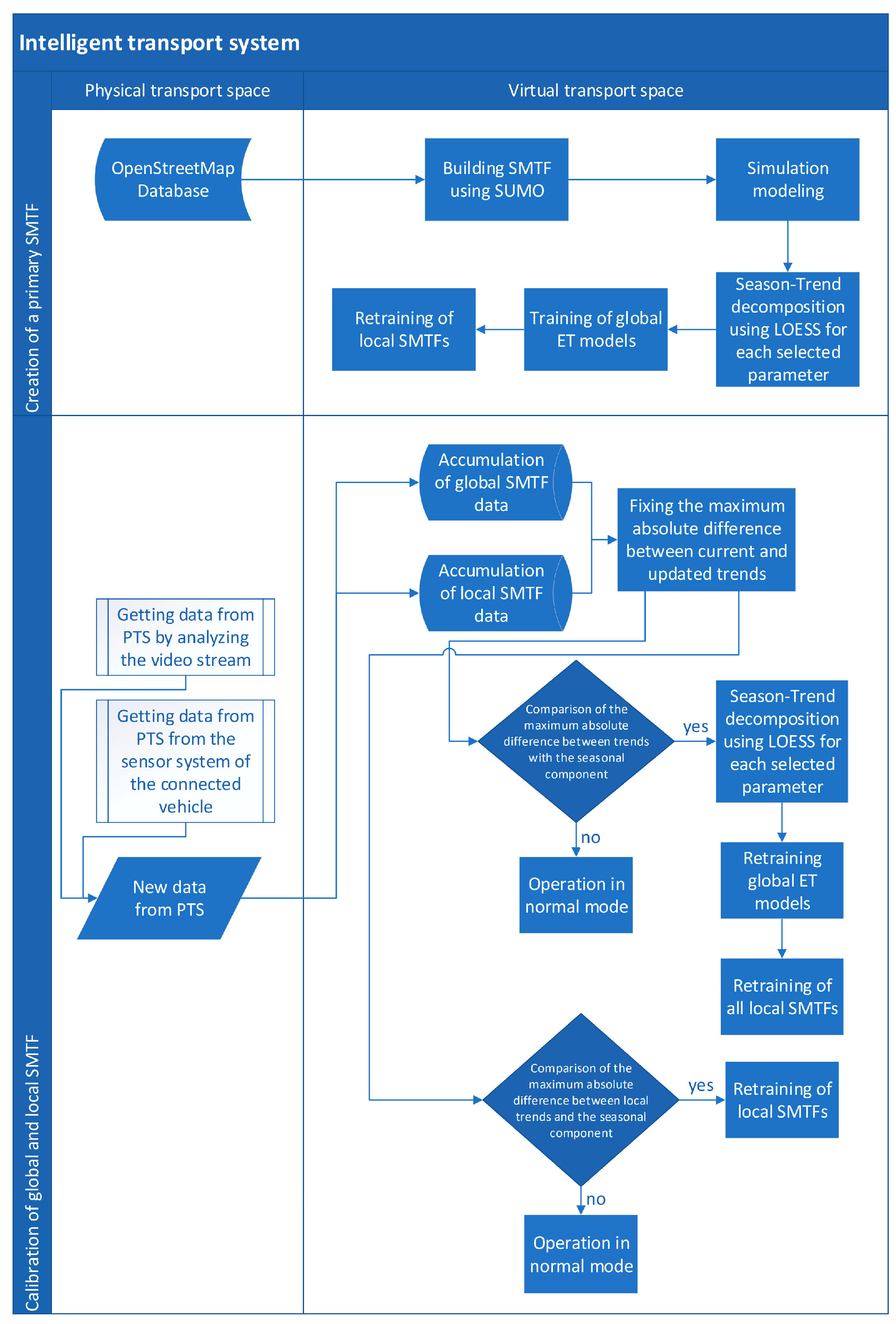
The interaction system between the PTS and the VTS, as shown in
Figure 3, includes an initial simulation model implemented in SUMO, divided into sectors with both initial global and several local patterns of SMTF timing characteristics. It also incorporates a monitoring system to track the updates of these global or local patterns.
Once the route graph is divided into sectors, an initial temporal dynamics pattern is established through three stages. The first stage involves initializing simulation modeling in SUMO, where fixed parameters are gathered in general and local databases for each sector. The second stage focuses on extracting the global time trend of
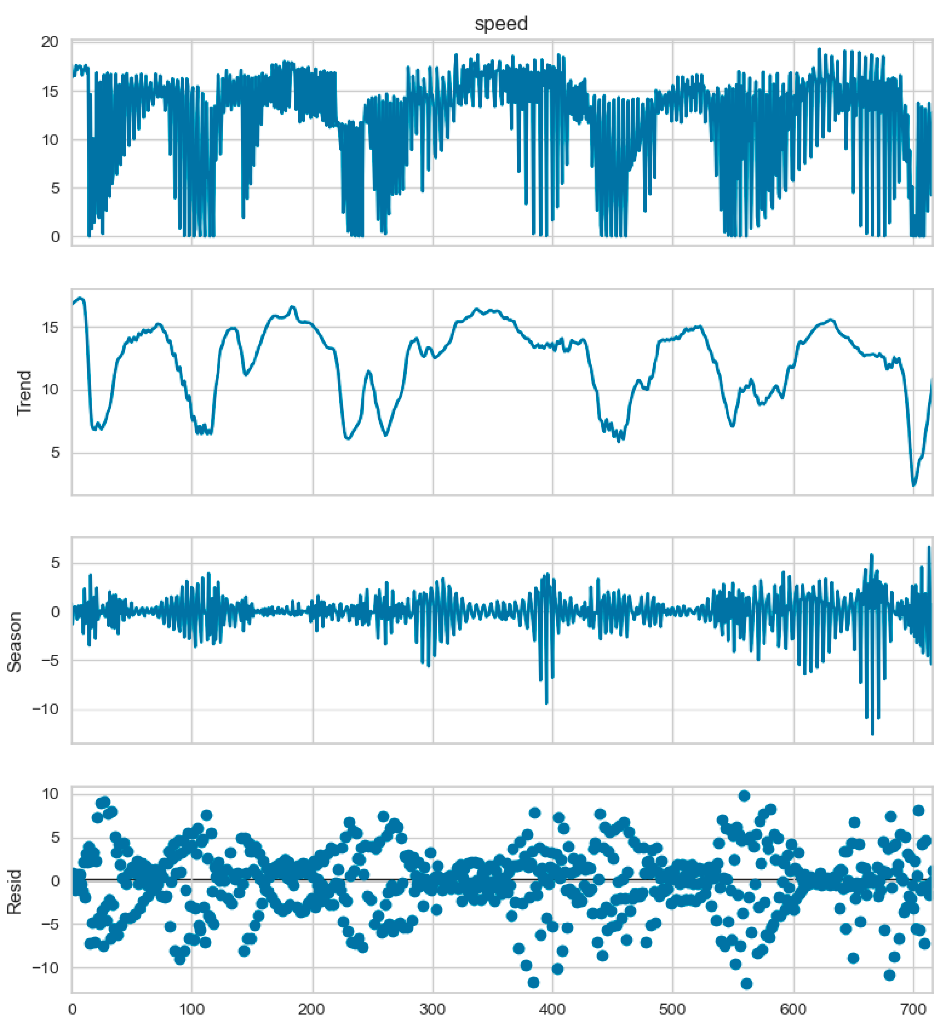
Yn for each of the n fixed parameters using a statistical method called seasonal trend decomposition using locally estimated scatterplot smoothing (LOESS) [
71].
By decomposing the time series of fixed parameter dynamics into seasonal, trend, and residual components, we can pinpoint the trend of the parameter Tn and the seasonal component
Sn. These components set the statistical proximity boundaries within which the calibration process of SMTF does not commence.
The resulting trend Tn is the foundation for training the global regression model. Additionally, the average duration of seasonal deviations τS was determined, representing the period during which Sn(t) values exceed half of its maximum value max(Sn).
The regression model was chosen based on three key criteria: high accuracy for variables with varying dynamics periods, computational complexity impacting training and retraining speed, and noise resistance to random short-term processes on the route. The Extra Trees Regressor (ET) algorithm was selected for the simulation because it met these criteria [
72].
As ET is an ensemble algorithm, a method was employed to adjust trained models considering regional drift to accelerate retraining [
69]. This involved updating models by incorporating new classifiers trained on new data while removing some older ones until reaching the desired accuracy threshold on the test sample selected during the calibration stage.
One advantage of ET is that it utilizes the average prediction from all trees in the ensemble, potentially reducing model variance compared to other ensemble algorithms when dealing with noisy data. Additionally, introducing an extra random process in selecting input parameter split points enhances data noise robustness [
73].
The third stage involves constructing the initial template of each cluster's dynamics through additional local training on the global ET model using the described ML model adjustment method within the local database of each sector.
Subsequently, the SMTF transitions into run mode while the data drift monitoring system continuously compares fixed parameter distributions over time. The SMTF generates data from ET models, allowing the calibration process to operate simultaneously.
When new data from the PTS is received (either from the video stream analysis system or from the connected vehicle's sensors), it is stored in the global database and then distributed to local databases based on the location of the vehicle when the data was collected. The accumulation of this new data from the PTS happens over a period of time denoted as τS.
Once the new data is collected, extracting key characteristics begins by calculating the trend of the new data and relevant test statistics. This involves determining the maximum absolute difference between two trends for comparison, denoted as max(Sn).
The decision to initiate global or local calibration is based on specific conditions:
If these conditions are met, additional training is conducted on the existing global ET model. The updated model is then incorporated into each sector by additional training on a local dataset, similar to the third stage of constructing the original SMTF. This additional model training occurs in parallel with the operation of the replaced models without causing any interruption. Additional training is only performed on a specific local model if a shift in local data is detected.
Evaluating the simulation's adherence to the established and calibrated SMTF involves a comprehensive process. It involves a statistically comparing the distributions of generated quantities with those obtained from the PTS data. Additionally, the performance of the ML algorithm, which has been extensively trained and integrated into the VTS, is assessed using a test dataset from the PTS. The results of these evaluations are presented in
Section 4.
3. Methodology for Analyzing Video Stream Data
In the Introduction, it was mentioned that data from stationary objects (such as video cameras) of road safety infrastructure, or sensors from vehicles connected to the WSN, are used to analyze the ITS transport situation. To create a flexible hybrid SMTF calibration system, separate preprocessing algorithms for each data source must be developed to represent the input data uniformly [
74,
75].
When preprocessing data from a connected vehicle sensor system, classical steps like data cleaning, integrating data from multiple vehicles in a time-sorted manner, and normalizing parameters under consideration may suffice [
76]. However, processing highway video monitoring data poses challenges in obtaining vehicle characteristics directly, which are crucial for many V2X ML applications. An additional algorithm is needed to extract vehicle characteristics from a video stream.
3.1. Algorithm for Extracting Traffic Data from a Video Stream
The data extraction algorithm involves three main steps:
Camera calibration and conversion of image coordinates to GNSS coordinates.
Tracking and calculation of spatiotemporal characteristics of vehicles.
Applying the Kalman filter to smooth the extracted values.
Initially, the YOLOv5 real-time video analytics system [
77] was used to analyze the video stream, detecting and tracking the movements of visible vehicles. The YOLO algorithm divides the original image into a grid of N × N cells. If the object’s center falls within the coordinates of a cell, then this cell is considered responsible for determining the object’s location parameters. Each object is defined by five values: center coordinates of the bounding box, its width, height, and confidence level that the box contains the object. For each object class-cell pair, the probability of the cell containing an object of that class must be determined.
The choice of YOLOv5 architecture was made for its high image processing speed and good object detection accuracy with minimal parameters and low learning rate. Training parameters included IoU threshold value of 0.5, image compression to 960 x 960 px, learning rate of 0.001, and SGD optimization algorithm. The training set comprised 3000 images, with 500 in the validation set.
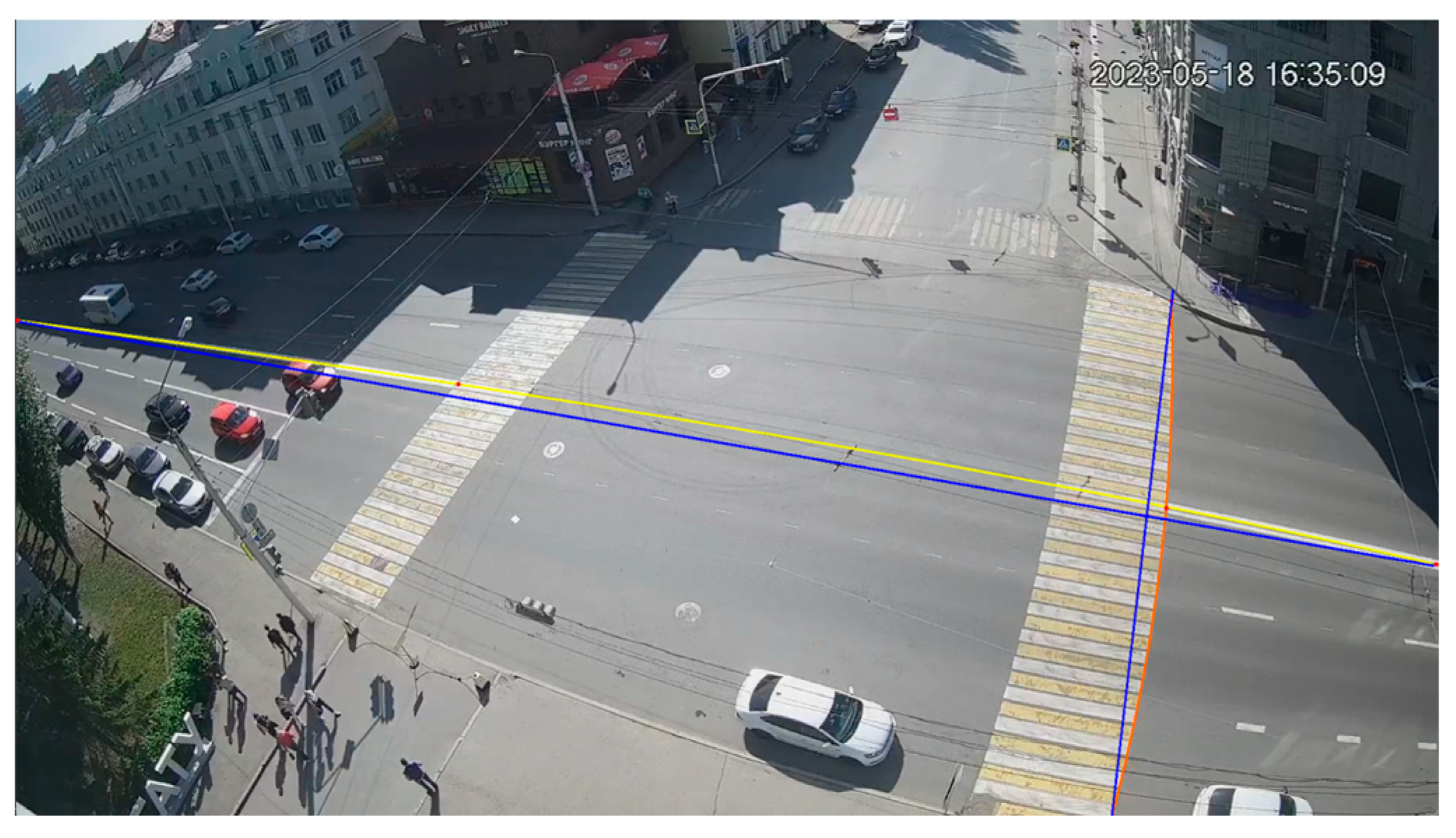
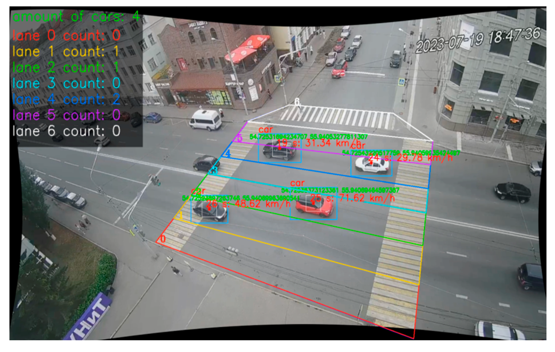
To accurately detect vehicles using YOLOv5 and analyze their parameters, it was essential to address the issue of image distortions caused by various factors and establish a method to convert image coordinates to GNSS coordinates.
Figure 4 shows an example of a distorted image.
To calibrate the camera images and map their coordinates to the GNSS coordinate system, the direct linear transformation (DLT) method [
78] was employed, along with the POSIT (Pose from Orthographic and Scaling with Iterations) method [
79] to calculate the position and orientation of vehicles. The necessary input data for these algorithms included details about the dimensions of the modeled area, reference points with known coordinates in both systems and information about the camera's optical configuration.
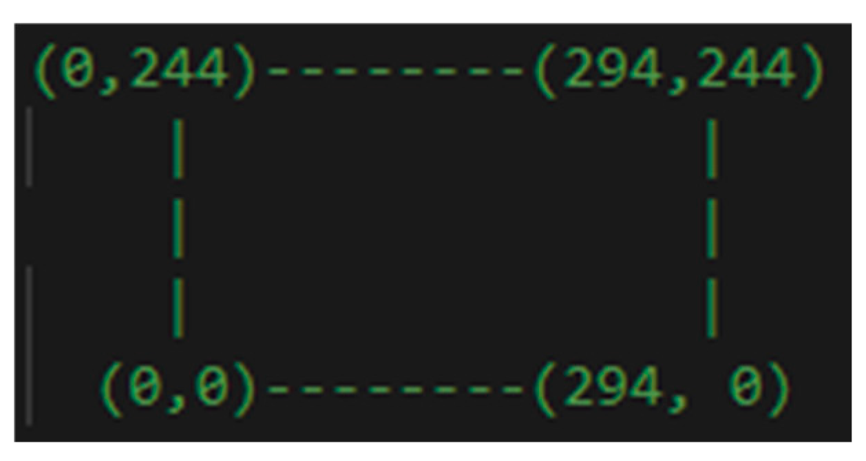
The specific section of the route that was simulated represented an intersection measuring 29.4 meters in width and 24.4 meters in length. Reference points were established in the camera coordinates to align with points in the intersection coordinate system: (0, 244), (0, 122), (0, 0), (147, 0), (294, 0), (294, 122), (294, 244), (147, 244).
A graphical representation of corner points from the intersection coordinate system is shown in
Figure 5.
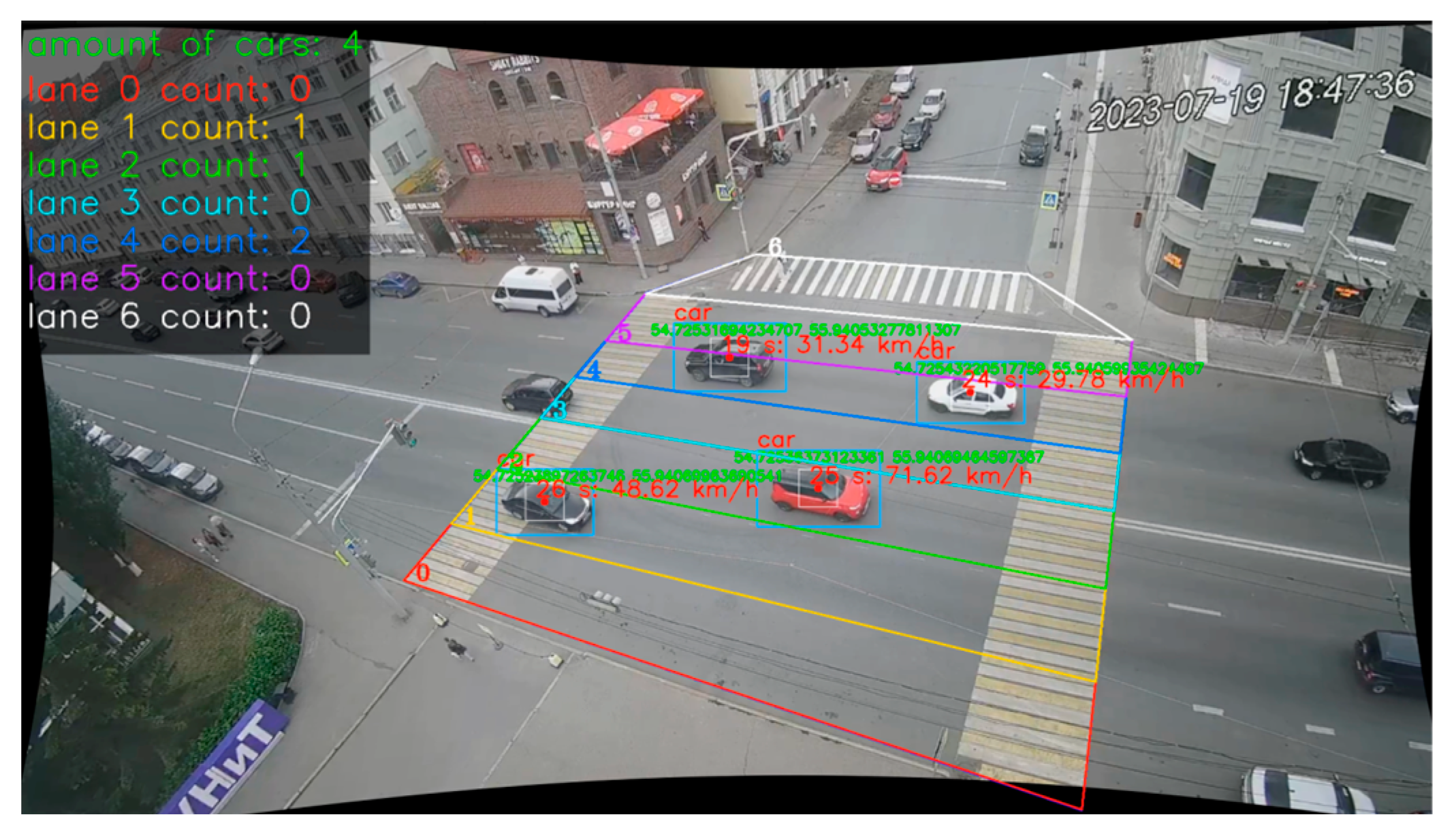
Frame marking was conducted after correcting distortions using the Nelder-Mead method implemented through the Python SciPy library in conjunction with the Python OpenCV library.
Figure 6 illustrates this process.
3.2. Tracking Algorithm and Indirect Calculation of Vehicle Characteristics
Four straight-line equations were formulated to define the boundaries of the visibility area along the route to improve the accuracy of tracking vehicle trajectories. The centers of objects within this area were identified in each frame, and the distances between these centers in consecutive frames were calculated using the Euclidean metric. When the distance traveled by a vehicle between frames exceeded a set threshold, its movement was recorded, and its trajectory was determined.
Figure 7 illustrates the movement of objects in frames
t1 and
t2.
The distance traveled in pixels between two frames for each object was used to calculate the speed of vehicles as an example of indirect characteristics. This distance allowed for determining the speed at the current time step:
where
d(...) is the calculation of the Euclidean metric, Ci is the selected object center coordinates on the frame's pixel grid, and FPS is the number of frames per second.
One-dimensional Kalman filtering was applied to all indirect characteristic calculations to provide a recursive estimation of the current speed value:
where
zk is the calculated speed value,
is the speed estimate at the previous step, and
KG is Kalman Gain, which is calculated:
where
EEST is the uncertainty of the current value estimate, and
EMEA is the tracking algorithm's error in calculating the speed.
4. Simulation Results of the SMTF Calibration Algorithm and Comparison of Results with PTS
The intersection of Karl Marx and Sverdlov streets in Ufa was chosen as a simulated section for creating and calibrating the SMTF. The coordinates of the video surveillance camera at this location are latitude 54.725376 and longitude 55.940998.
Using OpenStreetMap (OSM) data, a SUMO model was developed with traffic parameters set to Through Traffic Factor = 5 and Count = 12. The initial simulation involved 5000 steps, divided into six parts to establish the SMTF and subsequent calibration during the initial simulation. For example, to extract an indirect parameter of vehicles, we chose the parameters of speed, time of signal transmission from the vehicle to the infrastructure object, and the vehicle's rotation angle relative to the geographic north.
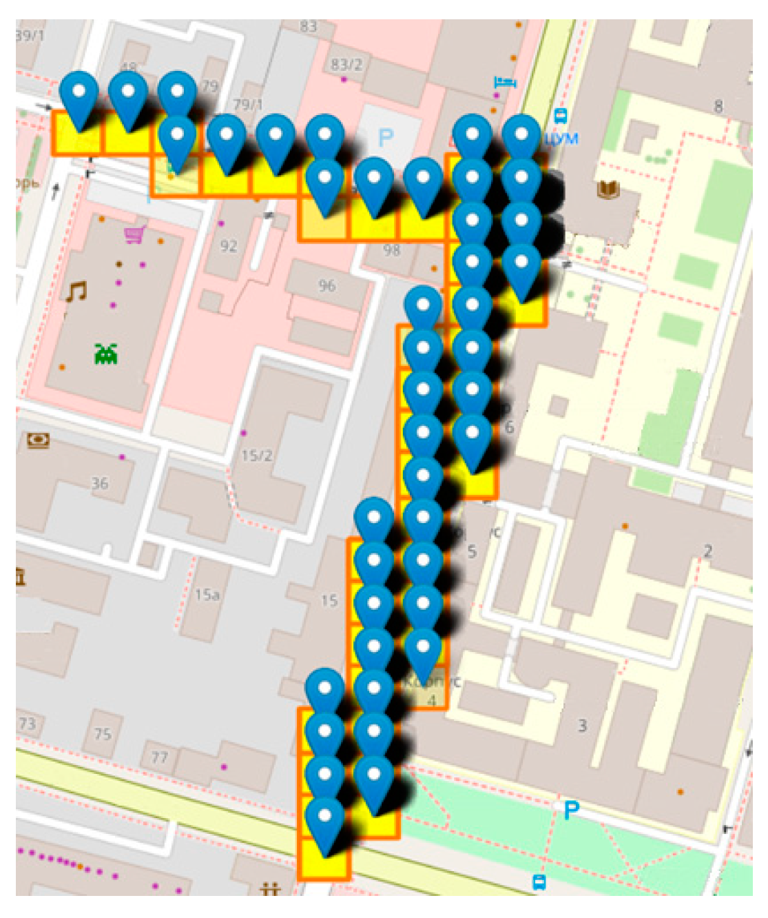
The simulated route area within a 600-meter radius from the camera location was divided into 40 sectors using Geohash coding (see
Figure 8).
Traffic speed trends were extracted using LOESS for the first 833 simulation steps (see
Figure 9). After averaging the calculated values of
τSn, a time interval
τS of 60 simulation steps was chosen, approximating a minute of real-time.
In subsequent five iterations generating new data from the SUMO model, the average global and local learning times were 3500 and 110 milliseconds, respectively. Global SMTF calibration initialization occurred in 5 out of 70 drift tracking iterations, while local calibration was observed in 26 cases.
After simulating the SMTF calibration, the model calibration was first tested based on data from an actual video stream of the PTS intersection. Of the 40 sectors in the new dataset, information was only available for six sectors in the center of the intersection. When initializing a new data drift monitoring cycle, global calibration of the model was not required due to a slight divergence in the trends of all parameters under consideration. Local calibration was initiated only for four sectors for the speed parameter, 2 for the signal transmission time parameter, and 1 for the rotation angle.
Data obtained directly from a moving vehicle in the simulated area was recorded using a programmable microcontroller ELM327 from ELM Electronics, which supports OBD-II protocols [
80] (p. 15031), to monitor vehicle data in real-time.
The performance of the calibration system was assessed by comparing data from the ELM327 and data generated by the SMTF before and after SMTF calibration. Two methods were used to compare the data: assessing the degree of statistical elimination of drift in data from the SMTF relative to the PTS and assessing the performance of the ML regression model trained on the SMTF data to determine the positions of the main lobe of the radiation pattern for establishing communication between the V2I infrastructure object and the vehicle.
To assess the statistical efficiency of SMTF calibration, the Kolmogorov-Smirnov (K-S) test was used, which is used to compare two samples to confirm that they belong to the same distribution [
81] (p. 14). The results of the K-S test showed a decrease in the maximum absolute difference between the distributions of the video stream data and the calibrated SMTF compared to the original model trained on SUMO data. An example of the original velocity distribution obtained from the SUMO model, the velocity distribution from the FTP, and the distribution after model calibration are presented in
Figure 10.
Thus, the results of the average level of reduction in the maximum absolute difference between the distributions of vehicle parameters are:
for the signal transmission time from the vehicle to the infrastructure object, a reduction of 37.64% was reached;
for vehicle speed, a reduction of 72.89% was achieved;
for the angle of rotation of the car relative to the geographic north, a reduction of 49.27% was acquired.
To test the stability of the phased array antenna beam steering algorithm when working with data from the PTS, input data, including the specified generated parameters, were created to train the ML model.
A special algorithm was developed to generate the target variable — the number of the sector in which the main lobe of the phased array antenna should be directed — in order to minimize connection delays and maintain a stable communication channel for the car. This algorithm associates clusters with sectors based on the vehicle's location at the time of connection to the V2I network or its movement through the simulated area. The algorithm generated random coordinates within the sector area and assigned properties to simulate a request to connect a vehicle.
Two identical ET models were trained after generating two SMTF data sets - before and after calibration. Their accuracy was assessed on ELM327 data using metrics to measure regression performance: mean absolute error (MAE), root mean square error (MSE), root mean square log error (RMSLE), coefficient of determination (
R2), and mean absolute percentage error (MAPE). The average cross-validation results on ELM327 data are presented in
Table 1.
A decrease in the MAE, MSE, RMSE, RMSLE, and MAPE metrics indicates a reduction in the discrepancy between the predicted directions of the main lobe of the radiation pattern and the vehicle's location. A significant increase in R2 indicates a decrease in the variance of the dependent variable relative to the independent ones, which indicates a decrease in data drift for the ML model integrated into the VTS.
The results confirm the effectiveness of the calibration algorithm based on global and local regression models and the vehicle data synthesis algorithm using YOLOv5-processed video stream data. Tests also show that the proposed method for extracting vehicle characteristics from a video stream allows data collection without creating a WSN, which requires upgrading city infrastructure and installing sensors on vehicles. This could reduce the costs of implementing urban ITS.
5. Discussion
The developed system for creating SMTF with the possibility of global and local calibration using data from the PTS has demonstrated high adaptability to temporal and spatial deviations from the actual dynamics of traffic flow. The algorithm for extracting vehicle characteristics from video stream analysis ensured high registration accuracy, which was confirmed by tests on the correspondence of the distributions of parameters of the data from the video stream analysis and from the sensor system of the test car (the K-S test will be carried out using data from the AI and the tracker).
In our future work, we plan to introduce a cluster formation algorithm to enhance the spatial accuracy of the simulation model. This algorithm will be based on the selection of elements of the simulated section of the path. Importantly, it will be designed to adapt their boundaries to the operation of specific VTS algorithms, such as the boundaries of the sectors of the beam steering algorithm of the phased array antenna, which plays a crucial role in our model.
An essential part of expanding the areas of application of SMTF will be integrating a microscopic traffic model into it, which will allow for simulation of the movement of specific vehicles within and between the cluster.
6. Conclusions
The proposed method for creating and calibrating a traffic simulation model showcased a significant increase in the statistical alignment between generated vehicle characteristics and actual car data on a simulated highway segment, improving from 37% to 73%. This enhancement was enabled by the approach's ability to calibrate the simulation model globally for overall trend changes and locally for specific route segments, offering flexibility and potentially saving time as local calibration could often replace global adjustments. Additionally, by reducing data drift for machine learning models integrated into the VTS system, the results indicate the algorithm's accuracy in synthesizing vehicle characteristics based on video traffic flow analysis. This capability eliminates the need to deploy WSN, potentially reducing the costs of implementing intelligent transportation systems.
Author Contributions
Conceptualization, E.L., E.G. and G.V.; methodology, E.L.; software, E.L. and A.A.; validation, E.L.; formal analysis, E.L., E.G. and G.V.; investigation, E.L. and A.A.; resources, E.L., E.G. and G.V.; data curation, E.L.; writing—original draft preparation, E.L.; writing—review and editing, E.G. and G.V.; visualization, E.L. and G.V.; supervision, E.G.; project adminis- tration, E.G.; funding acquisition, E.G. All authors have read and agreed to the published version of the manuscript.
Funding
This work was funded under the grant of the Russian Science Foundation (Project №21-79- 10407).
Institutional Review Board Statement
Not applicable.
Informed Consent Statement
Not applicable.
Data Availability Statement
A dataset for training the ML algorithm is available on request to the corresponding author’s e-mail.
Conflicts of Interest
The authors declare no conflict of interest.
Sample Availability
Not applicable.
References
- J. D. Bronzino and D. R. Peterson, Eds., ‘Medical Devices and Human Engineering’, CRC Press, Oct. 2018. [CrossRef]
- A. Statsenko, A. A. A. Statsenko, A. A. Rogov, I. V. Obukhov, and E. E. Smirnova, ‘Developing Software and Hardware for Automation of Ground Urban Transport Traffic Management’, 2021 IEEE Conference of Russian Young Researchers in Electrical and Electronic Engineering (ElConRus), pp. 1102–1105, Jan. 2021. [Google Scholar] [CrossRef]
- W. Mommad Salah and Z. Tie Gang, ‘Comparison of Hospital Logistics Systems’, IJSRP, vol. 11, no. 2, pp. 696–708, Feb. 2021. [CrossRef]
- J. Jin et al., ‘An Agent-Based Traffic Recommendation System: Revisiting and Revising Urban Traffic Management Strategies’, IEEE Transactions on Systems, Man, and Cybernetics: Systems, vol. 52, no. 11, pp. 7289–7301, Nov. 2022. [CrossRef]
- V. Vukadinovic et al., ‘3GPP C-V2X and IEEE 802.11p for Vehicle-to-Vehicle communications in highway platooning scenarios’, Ad Hoc Networks, vol. 74, pp. 17–29, May 2018. [CrossRef]
- X. Liao et al., ‘Game Theory-Based Ramp Merging for Mixed Traffic With Unity-SUMO Co-Simulation’, IEEE Transactions on Systems, Man, and Cybernetics: Systems, vol. 52, no. 9, pp. 5746–5757, Sep. 2022. [CrossRef]
- J. Wang, L. J. Wang, L. Bi, and W. Fei, ‘Multitask-Oriented Brain-Controlled Intelligent Vehicle Based on Human–Machine Intelligence Integration’, IEEE Transactions on Systems, Man, and Cybernetics: Systems, vol. 53, no. 4, pp. 2510–2521, Apr. 2023. [Google Scholar] [CrossRef]
- Z. Hu, S. Z. Hu, S. Lou, Y. Xing, X. Wang, D. Cao, and C. Lv, ‘Review and Perspectives on Driver Digital Twin and Its Enabling Technologies for Intelligent Vehicles’, IEEE Transactions on Intelligent Vehicles, vol. 7, no. 3, pp. 417–440, Sep. 2022. [Google Scholar] [CrossRef]
- G.-L. Huang, A. G.-L. Huang, A. Zaslavsky, S. W. Loke, A. Abkenar, A. Medvedev, and A. Hassani, ‘Context-Aware Machine Learning for Intelligent Transportation Systems: A Survey’, IEEE Transactions on Intelligent Transportation Systems, vol. 24, no. 1, pp. 17–36, Jan. 2023. [Google Scholar] [CrossRef]
- H. Zhang, G. H. Zhang, G. Luo, Y. Li, and F.-Y. Wang, ‘Parallel Vision for Intelligent Transportation Systems in Metaverse: Challenges, Solutions, and Potential Applications’, IEEE Transactions on Systems, Man, and Cybernetics: Systems, vol. 53, no. 6, pp. 3400–3413, Jun. 2023. [Google Scholar] [CrossRef]
- M. Treiber and A. Kesting, Traffic Flow Dynamics: Data, Models and Simulation, vol. 67. Springer Berlin, Heidelberg, 2013. Accessed: Mar. 13, 2024. [Online]. Available: https://pubs.aip.org/physicstoday/article/67/3/54/1017356/Traffic-Flow-Dynamics-Data-Models-and-
Simulation.
- Samarqand davlat universiteti, F. M Nazarov, B. Sh Eshtemirov, and Q. Sh Saydullayev, ‘Microscopic and macroscopic flow models of traffic management’, tips, vol. 1, no. 1, pp. 1–11, Feb. 2023. [Google Scholar] [CrossRef]
- P. A. Lopez et al., ‘Microscopic Traffic Simulation using SUMO’, in 2018 21st International Conference on Intelligent Transportation Systems (ITSC), Nov. 2018, pp. 2575–2582. [CrossRef]
- S. Wang, D. S. Wang, D. Yu, X. Ma, and X. Xing, ‘Analyzing urban traffic demand distribution and the correlation between traffic flow and the built environment based on detector data and POIs’, European Transport Research Review, Dec. 2018. [Google Scholar] [CrossRef]
- E. Lopukhova, A. E. Lopukhova, A. Abdulnagimov, G. Voronkov, R. Kutluyarov, and E. Grakhova, ‘Universal Learning Approach of an Intelligent Algorithm for Non-GNSS Assisted Beamsteering in V2I Systems’, Information, vol. 14, no. 2, Art. no. 2, Feb. 2023. [Google Scholar] [CrossRef]
- D. Krajzewicz, J. Erdmann, M. Behrisch, and L. Bieker, ‘Recent Development and Applications of SUMO -
Simulation of Urban MObility’, Dec. 2012. Accessed: Mar. 16, 2024. [Online]. Available:
https://www.semanticscholar.org/paper/Recent-Development-and-Applications-of-SUMO-of-Krajzewicz-
Erdmann/0e62ded610aeb17cc65f9f7159477e48248a98a2.
- Z. Szendrei, N. Z. Szendrei, N. Varga, and L. Bokor, ‘A SUMO-Based Hardware-in-the-Loop V2X Simulation Framework for Testing and Rapid Prototyping of Cooperative Vehicular Applications’, K. Jármai and B. Bolló, Eds., in Lecture Notes in Mechanical Engineering. Cham: Springer International Publishing, 2018, pp. 426–440. [CrossRef]
- C. Antoniou, M. C. Antoniou, M. Ben-Akiva, and H. N. Koutsopoulos, ‘Online Calibration of Traffic Prediction Models’, Transportation Research Record, vol. 1934, no. 1, pp. 235–245, Jan. 2005. [Google Scholar] [CrossRef]
- D. Salles, S. Kaufmann, and H.-C. Reuss, ‘Extending the Intelligent Driver Model in SUMO and Verifying the Drive Off Trajectories with Aerial Measurements’, SUMO Conference Proceedings, vol. 1, pp. 1–25, 2020. [CrossRef]
- M. Ross, L. M. Ross, L. Du, and B. Seibold, ‘Spatial-Temporal EV Charging Demand Model Considering Generic Second-Order Traffic Flows’, in 2021 IEEE Transportation Electrification Conference & Expo (ITEC), Jun. 2021, pp. 789–794. [CrossRef]
- H. Hashemi and K. Abdelghany, ‘Integrated Method for Online Calibration of Real-Time Traffic Network Management Systems’, Transportation Research Record, vol. 2528, no. 1, pp. 106–115, Jan. 2015. [CrossRef]
- Keler, A. Kunz, S. Amini, and K. Bogenberger, ‘Calibration of a Microscopic Traffic Simulation in an Urban Scenario Using Loop Detector Data: A Case Study within the Digital Twin Munich’, SUMO Conf Proc, vol. 4, p. 153, Jun. 2023. [Google Scholar] [CrossRef]
- Bamdad Mehrabani, L. Sgambi, S. Maerivoet, and M. Snelder, ‘Development, Calibration, and Validation of a Large-Scale Traffic Simulation Model: Belgium Road Network’, SUMO Conf Proc, vol. 4, pp. 15–27, Jun. 2023. [Google Scholar] [CrossRef]
- J. J. Gonzalez-Delicado, J. Gozalvez, J. Mena-Oreja, M. Sepulcre, and B. Coll-Perales, ‘Alicante-Murcia Freeway Scenario: A High-Accuracy and Large-Scale Traffic Simulation Scenario Generated Using a Novel Traffic Demand Calibration Method in SUMO’, IEEE Access, vol. 9, pp. 154423–154434, 2021. [CrossRef]
- R. Balakrishna, C. R. Balakrishna, C. Antoniou, M. Ben-Akiva, H. N. Koutsopoulos, and Y. Wen, ‘Calibration of Microscopic Traffic Simulation Models: Methods and Application’, Transportation Research Record, vol. 1999, no. 1, pp. 198–207, Jan. 2007. [Google Scholar] [CrossRef]
- M. J. Lighthill and G. B. Whitham, ‘On kinematic waves II. A theory of traffic flow on long crowded roads’, Proceedings of the Royal Society of London. Series A. Mathematical and Physical Sciences, vol. 229, no. 1178, pp. 317–345, Jan. 1997. [CrossRef]
- L. Huang, S.-N. L. Huang, S.-N. Zhang, S.-B. Li, F.-Y. Cui, J. Zhang, and T. Wang, ‘Phase transition of traffic congestion in lattice hydrodynamic model: Modeling, calibration and validation’, Mod. Phys. Lett. B, vol. 38, no. 08, p. 2450012, Mar. 2024. [Google Scholar] [CrossRef]
- S. Y. R. Rompis, F. G. S. Y. R. Rompis, F. G. Habtemichael, Department of Civil Engineering, Sam Ratulangi University, Indonesia, and National Center for Sustainable Transportation Technology, Indonesia, ‘Calibration of Traffic Incident Simulation Models Using Field Data’, IJSTT, vol. 2, no. 1, pp. 19–26, Apr. 2019. [Google Scholar] [CrossRef]
- N. Dadashzadeh, M. Ergun, A. S. Kesten, and M. Zura, ‘Improving the calibration time of traffic simulation models using parallel computing technique’, 2019 6th International Conference on Models and Technologies for Intelligent Transportation Systems (MT-ITS), pp. 1–7, Jun. 2019. [CrossRef]
- C. Cobos et al., ‘Multi-objective Memetic Algorithm Based on NSGA-II and Simulated Annealing for Calibrating CORSIM Micro-Simulation Models of Vehicular Traffic Flow’, O. Luaces, J. A. Gámez, E. Barrenechea, A. Troncoso, M. Galar, H. Quintián, and E. Corchado, Eds., in Lecture Notes in Computer Science, vol. 9868. Cham: Springer International Publishing, 2016, pp. 468–476. [CrossRef]
- M. Yu and W. (David) Fan, ‘Calibration of microscopic traffic simulation models using metaheuristic algorithms’, International Journal of Transportation Science and Technology, vol. 6, no. 1, pp. 63–77, Jun. 2017. [CrossRef]
- F. Storani, R. F. Storani, R. Di Pace, F. Bruno, and C. Fiori, ‘Analysis and comparison of traffic flow models: a new hybrid traffic flow model vs benchmark models’, Eur. Transp. Res. Rev., vol. 13, no. 1, p. 58, Dec. 2021. [Google Scholar] [CrossRef]
- Y. Imai, H. Y. Imai, H. Fujii, K. Okano, M. Matsudaira, and T. Suzuki, ‘Development of Dynamic Micro- and Macroscopic Hybrid Model for Efficient Highway Traffic Simulation: Model Extension to Merging Sections and Validation with Probe Data’, Int. J. ITS Res., Feb. 2024. [Google Scholar] [CrossRef]
- W. Burghout, H. N. W. Burghout, H. N. Koutsopoulos, and I. Andréasson, ‘Hybrid Mesoscopic–Microscopic Traffic Simulation’, Transportation Research Record, vol. 1934, no. 1, pp. 218–225, Jan. 2005. [Google Scholar] [CrossRef]
- E. Bourrel and J.-B. Lesort, ‘Mixing Microscopic and Macroscopic Representations of Traffic Flow: Hybrid Model Based on Lighthill–Whitham–Richards Theory’, Transportation Research Record, vol. 1852, no. 1, pp. 193–200, Jan. 2003. [CrossRef]
- E. Bourrel and J. Lesort, ‘Mixing Micro and Macro Representations of Traffic Flow: a Hybrid Model Based on the LWR Theory’, 2003. Accessed: Mar. 12, 2024. [Online]. Available: https://www.semanticscholar.org/paper/Mixing-Micro-and-Macro-Representations-of-Traffic-a-Bourrel-Lesort/9f5d08d4f35180a9b3d2dd2385a036910fba626d.
- L. Magne, S. Rabut, J. Gabard, and O. Toulouse, ‘Towards an hybrid macro-micro traffic flow simulation model’, 2000. Accessed: Mar. 12, 2024. [Online]. Available: https://www.semanticscholar.org/paper/Towards-an-hybrid-macro-micro-traffic-flow-model-Magne-Rabut/7b073b5a3cede03297e383cea558559a920623d0.
- Würth, M. Binois, and P. Goatin, ‘Traffic prediction by combining macroscopic models and Gaussian processes’, Dec. 2023. Accessed: Mar. 13, 2024. [Online]. Available: https://hal.science/hal-04345140.
- Sroczyński and, A. Czyżewski, ‘Road traffic can be predicted by machine learning equally effectively as by complex microscopic model’, Sci Rep, vol. 13, no. 1, p. 14523, Sep. 2023. [Google Scholar] [CrossRef]
- S. Son, Y.-L. Qiao, J. Sewall, and M. C. Lin, ‘Differentiable Hybrid Traffic Simulation’, ACM Trans. Graph., vol. 41, no. 6, p. 258:1-258:10, Nov. 2022. [CrossRef]
- S. Das and I. Tsapakis, ‘Interpretable machine learning approach in estimating traffic volume on low-volume roadways’, International Journal of Transportation Science and Technology, vol. 9, no. 1, pp. 76–88, Mar. 2020. [CrossRef]
- W. Xu and H. Wei, ‘Learning to Calibrate Hybrid Hyperparameters: a Study on Traffic Simulation’, ACM SIGSIM Conference on Principles of Advanced Discrete Simulation, pp. 144–147, Jun. 2023. [CrossRef]
- Shubhi and A. K. Singh, ‘Wireless Sensor Network: A Survey’, 2015. Accessed: Mar. 15, 2024. [Online]. Available: https://www.semanticscholar.org/paper/Wireless-Sensor-Network%3A-A-Survey-Shubhi-Singh/e50fa8e34a945367699dc33833def3e2a507127c.
- Das, M. Desai, N. Mugatkar, and A. S. Ponraj, ‘Emergency and Traffic Congestion Avoidance Using Vehicle-to-Vehicle Communication’, D. Thalmann, N. Subhashini, K. Mohanaprasad, and M. S. B. Murugan, Eds., in Lecture Notes in Electrical Engineering, vol. 492. Singapore: Springer Singapore, 2018, pp. 147–153. [CrossRef]
- H. Yu and M. Guo, ‘An Efficient Freeway Traffic Information Monitoring Systems Based on Wireless Sensor Networks and Floating Vehicles’, 2010 First International Conference on Pervasive Computing, Signal Processing and Applications, pp. 1065–1068, Sep. 2010. [CrossRef]
- W. Qua, ‘Compressed Sensing for Data Collection in Wireless Sensor Network’, Chinese Journal of Sensors and Actuators, 2014, Accessed: Mar. 15, 2024. [Online]. Available: https://www.semanticscholar.org/paper/Compressed-Sensing-for-Data-Collection-in-Wireless-Qua/b29aeb410ae4c88b73dcfe088bb4bdc6e5eac6fb.
- H. Wang, M. Ouyang, Q. Meng, and Q. Kong, ‘A traffic data collection and analysis method based on wireless sensor network’, J Wireless Com Network, vol. 2020, no. 1, p. 2, Dec. 2020. [CrossRef]
- A. Mednis, G. Strazdins, M. Liepins, A. Gordjusins, and L. Selavo, ‘RoadMic: Road Surface Monitoring Using Vehicular Sensor Networks with Microphones’, F. Zavoral, J. Yaghob, P. Pichappan, and E. El-Qawasmeh, Eds., in Communications in Computer and Information Science, vol. 88. Berlin, Heidelberg: Springer Berlin Heidelberg, 2010, pp. 417–429. [CrossRef]
- Prof. H. S. Goliya, ‘Data Collection and Modeling of Heterogeneous Traffic – A Review’, IJRASET, vol. 6, no. 3, pp. 1765–1767, Mar. 2018. [CrossRef]
- J. Hourdakis, P. G. Michalopoulos, and T. Morris, ‘Deployment of Wireless Mobile Detection and Surveillance for Data-Intensive Applications’, Transportation Research Record, vol. 1900, no. 1, pp. 140–148, Jan. 2004. [CrossRef]
- M. Manjusha and V. Sunitha, ‘A review of advanced pavement distress evaluation techniques using unmanned aerial vehicles’, International Journal of Pavement Engineering, vol. 24, no. 2, p. 2268796, Jan. 2023. [CrossRef]
- S.-S. Park, V.-T. Tran, and D.-E. Lee, ‘Application of Various YOLO Models for Computer Vision-Based Real-Time Pothole Detection’, Applied Sciences, vol. 11, no. 23, p. 11229, Nov. 2021. [CrossRef]
- P. Hidas and P. Wagner, ‘Review of Data Collection Methods for Microscopic Traffic Simulation’, 2004. Accessed: Mar. 15, 2024. [Online]. Available: https://www.semanticscholar.org/paper/Review-of-Data-Collection-Methods-for-Microscopic-Hidas-Wagner/f089b5ee5358d243762e1aaa143d057275629573.
- J. Apeltauer, A. Babinec, D. Herman, and T. Apeltauer, ‘AUTOMATIC VEHICLE TRAJECTORY EXTRACTION FOR TRAFFIC ANALYSIS FROM AERIAL VIDEO DATA’, Int. Arch. Photogramm. Remote Sens. Spatial Inf. Sci., vol. XL-3/W2, pp. 9–15, Mar. 2015. [CrossRef]
- Technical engineering collage, Northren technical university (NTU), Mosul, Iraq et al., ‘Multimedia Imaging System of Data Collection and Antenna Alignment for Unmanned Aerial Vehicles Based Internet of Things’, FPA, vol. 12, no. 2, pp. 19–27, 2023. [CrossRef]
- L. Kornyei, Z. Horvath, A. Ruopp, A. Kovacs, and B. Liszkai, ‘Multi-scale Modelling of Urban Air Pollution with Coupled Weather Forecast and Traffic Simulation on HPC Architecture’, The International Conference on High Performance Computing in Asia-Pacific Region Companion, pp. 9–10, Jan. 2021. [CrossRef]
- Basnayake, A. MacIver, and G. Lachapelle, ‘A GPS-BASED CALIBRATION TOOL FOR MICROSCOPIC TRAFFIC SIMULATION MODELS’, 2003. Accessed: Mar. 16, 2024. [Online]. Available: https://www.semanticscholar.org/paper/A-GPS-BASED-CALIBRATION-TOOL-FOR-MICROSCOPIC-MODELS-Basnayake-MacIver/d3c55875a982f39a94664e557d53700602547b0b.
- M. Barsi and A. Barsi, ‘BUILDING OPENDRIVE MODEL FROM MOBILE MAPPING DATA’, Int. Arch. Photogramm. Remote Sens. Spatial Inf. Sci., vol. XLIII-B4-2021, pp. 9–14, Jun. 2021. [CrossRef]
- E. J. Oughton, T. Russell, J. Johnson, C. Yardim, and J. Kusuma, ‘itmlogic: The Irregular Terrain Model by Longley and Rice’, Journal of Open Source Software, vol. 5, no. 51, p. 2266, Jul. 2020. [CrossRef]
- G. Savitha, R. S. Murthy, H. S. Jagadeesh, H. S. Sathish, and T. Sundararajan, ‘Study on Geometric Factors Influencing Saturation Flow Rate at Signalized Intersections under Heterogeneous Traffic Conditions’, JTTs, vol. 07, no. 01, pp. 83–94, 2017. [CrossRef]
- F. Zhang, Y. Qian, and J. Zeng, ‘Characterizing Heterogeneous Traffic Flow at a Slope Bottleneck via Cellular Automaton Model’, IEEE Trans. Intell. Transport. Syst., vol. 24, no. 6, pp. 6507–6516, Jun. 2023. [CrossRef]
- W. Ai, J. Hu, and D. Liu, ‘Bifurcation Analysis of Improved Traffic Flow Model on Curved Road’, Journal of Computational and Nonlinear Dynamics, vol. 18, no. 7, p. 071005, Jul. 2023. [CrossRef]
- G. Guido et al., ‘Evaluation of Contributing Factors Affecting Number of Vehicles Involved in Crashes Using Machine Learning Techniques in Rural Roads of Cosenza, Italy’. Dec. 20, 2021. [CrossRef]
- H. Al-Bayati, A. S. Shakoree, and Z. A. Ramadan, ‘Factors Affecting Traffic Accidents Density on Selected Multilane Rural Highways’, Civ Eng J, vol. 7, no. 7, pp. 1183–1202, Jul. 2021. [CrossRef]
- D. Zakharov, E. Magaril, and E. Rada, ‘Sustainability of the Urban Transport System under Changes in Weather and Road Conditions Affecting Vehicle Operation’, Sustainability, vol. 10, no. 6, p. 2052, Jun. 2018. [Google Scholar] [CrossRef]
- Y. Cui and S. S. Ge, ‘Autonomous vehicle positioning with GPS in urban canyon environments’, IEEE Transactions on Robotics and Automation, vol. 19, no. 1, pp. 15–25, Feb. 2003. [CrossRef]
- J. Meguro, T. Murata, J. Takiguchi, Y. Amano, and T. Hashizume, ‘GPS Multipath Mitigation for Urban Area Using Omnidirectional Infrared Camera’, IEEE Transactions on Intelligent Transportation Systems, vol. 10, no. 1, pp. 22–30, Mar. 2009. [CrossRef]
- Z. Ji and Q. Xie, ‘Bidirectional Mapping Trajectory Similarity Measurement Algorithm Based on Geohash Grid’, 2021 6th International Symposium on Computer and Information Processing Technology (ISCIPT), pp. 281–285, Jun. 2021. [CrossRef]
- J. Lu, A. Liu, F. Dong, F. Gu, J. Gama, and G. Zhang, ‘Learning under Concept Drift: A Review’, IEEE Transactions on Knowledge and Data Engineering, vol. 31, no. 12, pp. 2346–2363, Dec. 2019. [CrossRef]
- K. Ostrowski and M. Budzynski, ‘Measures of Functional Reliability of Two-Lane Highways’, Energies, vol. 14, no. 15, p. 4577, Jul. 2021. [CrossRef]
- R. Cleveland, ‘STL : A Seasonal-Trend Decomposition Procedure Based on Loess’, 1990. Accessed: Mar. 17, 2024. [Online]. Available: https://www.semanticscholar.org/paper/STL-%3A-A-Seasonal-Trend-Decomposition-Procedure-on-Cleveland/585bf445ec84c1d9621b2726bdcce9f544b515c8.
- S. Arjasakusuma, S. Swahyu Kusuma, and S. Phinn, ‘Evaluating Variable Selection and Machine Learning Algorithms for Estimating Forest Heights by Combining Lidar and Hyperspectral Data’, IJGI, vol. 9, no. 9, p. 507, Aug. 2020. [CrossRef]
- S. Martiello Mastelini, F. K. Nakano, C. Vens, and A. C. P. de Leon Ferreira de Carvalho, ‘Online Extra Trees Regressor’, IEEE Trans Neural Netw Learn Syst, vol. 34, no. 10, pp. 6755–6767, Oct. 2023. [CrossRef]
- J. Kim, H. Hwangbo, and S. Kim, ‘An empirical study on real-time data analytics for connected cars: Sensor-based applications for smart cars’, International Journal of Distributed Sensor Networks, vol. 14, no. 1, p. 155014771875529, Jan. 2018. [CrossRef]
- H. Al-Ahmadi, H. Hassan, and Al-Ahmadi, ‘Real-Time Simulation of Traffic Monitoring System in Smart City’, 2020. Accessed: Mar. 12, 2024. [Online]. Available: https://www.semanticscholar.org/paper/Real-Time-Simulation-of-Traffic-Monitoring-System-Al-Ahmadi-Hassan/fbd7a10eda11b03614e3a319a867c2e2f8d7ebe7.
- K. Mallikharjuna Rao, G. Saikrishna, and K. Supriya, ‘Data preprocessing techniques: emergence and selection towards machine learning models - a practical review using HPA dataset’, Multimed Tools Appl, vol. 82, no. 24, pp. 37177–37196, Oct. 2023. [CrossRef]
- N. Algiriyage et al., Towards Real-time Traffic Flow Estimation using YOLO and SORT from Surveillance Video Footage. 2021.
- F. Barone, M. Marrazzo, and C. J. Oton, ‘Camera Calibration with Weighted Direct Linear Transformation and Anisotropic Uncertainties of Image Control Points’, Sensors (Basel), vol. 20, no. 4, p. 1175, Feb. 2020. [Google Scholar] [CrossRef]
- D. F. Dementhon and L. S. Davis, ‘Model-based object pose in 25 lines of code’, Int J Comput Vision, vol. 15, no. 1–2, pp. 123–141, Jun. 1995. [CrossRef]
- 14:00-17:00, ‘ISO 15031-5:2015’, ISO. Accessed: Apr. 03, 2024. [Online]. Available: https://www.iso.org/standard/66368.html.
- R. H. Riffenburgh, ‘Chapter 14 - Tests on Variability and Distributions’, in Statistics in Medicine (Third Edition), R. H. Riffenburgh, Ed., San Diego: Academic Press, 2012, pp. 299–323. [CrossRef]
|
Disclaimer/Publisher’s Note: The statements, opinions and data contained in all publications are solely those of the individual author(s) and contributor(s) and not of MDPI and/or the editor(s). MDPI and/or the editor(s) disclaim responsibility for any injury to people or property resulting from any ideas, methods, instructions or products referred to in the content. |
© 2024 by the authors. Licensee MDPI, Basel, Switzerland. This article is an open access article distributed under the terms and conditions of the Creative Commons Attribution (CC BY) license (http://creativecommons.org/licenses/by/4.0/).
