Submitted:
04 May 2024
Posted:
06 May 2024
You are already at the latest version
Abstract
Here we compile a detailed record of eddies and examine their intra-annual variability over the Spitsbergen Bank in the northwestern Barents Sea using spaceborne Sentinel-1 A/B synthetic aperture radar (SAR) data acquired in 2018. Analysis of 3070 SAR images enabled to register 1758 eddy manifestations in the marginal ice zone (MIZ) and 1631 signatures in the open water (OW). Submesoscale and small mesoscale eddies were observed within a range 0.2-40 km with the range of MIZ eddies being twice larger than that of OW eddies. We note a strong seasonal variability of eddy diameters and the ratio of cyclones to anticyclones. The eddies were present in all seasons showing an approximate parity in eddy generation intensity in the surface layer between winter and summer. The peak eddy activity is observed during the first (January to March) and third (July-September) quarters of the year. A well-pronounced seasonality of SAR-derived eddy intensity correlates with that of eddy kinetic energy in the surface layer of the Eurasian Arctic. Eddies were detected most frequently in Storfjorden, south of Edge Island, near Hopen Island and along the entire eastern flank of the Spitsbergen Bank. Very low eddy activity was observed in the central part of the bank. The MIZ eddies were recorded during eight months of the year peaking in February, and being spatially limited by a 200-m isobath. The OW eddies were widely dispersed across the study domain peaking in August and tending to accumulate in regions of relatively weak surface currents. In summer, about 20-25% of them were observed within the Barents Sea Polar Front.
Keywords:
ocean eddies
; open water regions
; marginal ice zone
; SAR imaging
; Sentinel-1
; Barents Sea
; Spitsbergen Bank
; Svalbard
; Edge Island
; Hopen Island
; Storfjorden
; Arctic Ocean
1. Introduction
Ocean eddies play an important role in intensification of mixing, horizontal and vertical transfer of heat and matter [Thomas et al., 2008; Zhong, Bracco, 2013]. Investigation of eddies is, therefore, important for understanding the mechanisms of redistribution and transport of heat, salt and biogeochemical parameters in the Arctic Ocean [Watanabe et al., 2014; von Appen et al., 2018; Pnyushkov et al., 2018; Bashmachnikov et al., 2023].
Investigation of eddy-related pumping of warm water from the Atlantic Water layer up to the mixed layer and sea ice is one of the important aspects of the current research in the Arctic with declining ice cover [Manucharyan, Thompson, 2022; von Appen et al., 2022; Rippeth, Fine, 2022; Mueller et al., 2024].
In recent decades, meso- and submesoscale eddy structures in the Arctic have been actively studied using various methods, including in situ measurements, numerical models and satellite observations [Zhao et al., 2014; Fine et al., 2018; Mensa et al., 2018; Porter et al., 2020; Platov, Golubeva, 2020; Kubryakov et al., 2021; Meneghello et al., 2021; Manucharyan, Thompson, 2022; Cassianides et al., 2023; Morozov, Kozlov, 2023; Mueller et al., 2024]. High-resolution observations of spaceborne synthetic aperture radars (SARs), transparent to clouds, proved to be the most effective to study fine-scale and submesoscale eddy processes in the Arctic [Atadzhanova et al., 2017; Kozlov et al., 2020; Khachatrian et al., 2023].
Here we focus on the north-western (NW) Barents Sea. Recent studies of the nearby regions showed an active eddy generation in the vicinity of Spitsbergen Bank [Fer, Drinkwater, 2014; Atadzhanova et al., 2018; Petrenko, Kozlov, 2020, 2023; Kozlov, Atadzhanova, 2022; Kolas et al., 2023]. The Spitsbergen Bank (SB) is the shallow region with depths less than 100 m extending between Bear Island (BI) and Hopen Island (HI) (Figure 1).
The SB area is unique for a number of reasons. Firstly, it has a seasonal ice cover that forms in winter. A maximum sea ice extent is observed here in April [Pavlova et al., 2013], while the southernmost position of the marginal ice zone (MIZ) does not advance southward of the southern SB border. Secondly, the bank is characterized by a presence of several current systems of Atlantic and Arctic origin (Figure 1). One of the major features here is a quasi-permanent Barents Sea Polar Front (PF) found along its southern slope as a result of interaction of warm salty Atlantic Water (AW, marked by red arrows in Figure 1) and cold less saline Polar Water (PW, marked by blue arrows in Fig. 1) [Loeng, 1991; Parsons et al., 1996]. The region is also known for pronounced depth gradients at the outer boundaries of the bank, and strong tidal currents [Fer et al., 2020; Marchenko et al., 2021; Kowalik, Marchenko, 2023]. All these features favor the formation of eddies here.
Recent studies also show that eddies forming near the PF could have a greater influence on the frontal zone properties compared to tidal processes [Kolas et al., 2023]. In particular, they could cause shifts in the position of the front and contribute to the seasonal variability of the upper layer. They can also cause a local increase in the mixing rate in the marginal ice zone [Fer, Sundfjord, 2007] and a local heterogeneity of phytoplankton [Porter et al., 2020; Koenig et al., 2024].
The aim of this study is to analyze the intensity of eddy generation and its seasonal variability, as well as to document eddy properties over the SB region spanning 73.7°–78.9° N and 16° E–30° E (Fig. 1) from year-round Sentinel-1 SAR observations in 2018.
2. Materials and Methods
To investigate eddy signatures over the SB, we analyze C-band SAR images acquired by SAR-C instrument onboard Sentinel-1A and Sentinel-1B satellites (hereinafter, S-1A/B) in January–December 2018. S-1A/B data were publicly available and obtained from Alaska Satellite Facility (https://search.asf.alaska.edu, accessed on 1 February 2023). For the analysis we use 3070 SAR images taken in Interferometric Wide swath and Extra-Wide swath modes with spatial resolution of 20 m and 90 m, respectively. The number of images available per given month varied from 180 to 281 images.
Figure 2a shows a spatial coverage of the study site by S-1A/B data in 2018. Due to intersection of S-1A and S-1B orbits, the data coverage is generally higher north of 76°N (see, e.g., Figure 1 in [Kozlov et al., 2020]). The maximal density of SAR observations, about 700 scenes per unit area, is found in the latitude band of 77°-78° N. The minimal data coverage is around BI in the southwestern part of the study region with about 400 SAR images per unit area.
In SAR images, surface manifestations of eddy structures over open water (OW) and marginal ice zone (MIZ) are formed owing to three main mechanisms related to wave/current interactions and accumulation of surface films or drifting ice in the surface current convergence zones associated with eddy dynamics [Johannessen et al., 1996, 2005; Gade et al., 2013; Kozlov et al., 2019].
At low winds (below 5 m/s), eddies usually appear in SAR images due to presence of natural films on the sea surface, which dampen capillary and short gravity waves [Johannessen et al., 1996; Karimova, 2012; Gade et al., 2013; Hamze-Ziabari et al., 2022]. Surfactant films are entrained by the orbital motion of eddies, which thereby are manifested in radar images as spiraling features [Munk et al., 2000], as shown in Figure 2b. At higher winds exceeding 5-7 m/s, eddies are seen in SAR images owing to wave-current interactions when bright curved lines are formed due to enhanced radar backscatter over breaking wind waves in zones of enhanced surface current shear [Johannessen et al., 2005; Kudryavtsev et al., 2014].
Much more pronounced and less dependent on background winds are SAR signatures of eddies forming in the MIZ. However, their SAR manifestations depend on geometric properties, primarily thickness and roughness, of drifting ice. In this case, thinner and relatively flat sea ice (e.g., newly forming or melting ice) would be seen in SAR images predominantly as dark patterns (low backscatter regions), while thicker and rough sea ice — as relatively bright patterns (regions of high backscatter). This is illustrated in Sentinel-1 image acquired on 12 February 2018 (Figure 2c).
Analysis of S-1A/B SAR data was performed using the open-source ESA SNAP software (http://step.esa.int/main/toolboxes/snap, accessed on 30 December 2022). The original SAR data were calibrated to normalized radar cross-section units and smoothed to reduce the speckle noise using Lee filter [Lee, 1983]. We recorded the following characteristics of eddies: center coordinates, diameter, sign of rotation – cyclone (C) or anticyclone (Ac), type of manifestation (open water or MIZ). Mean spatial properties of eddies were calculated on a grid of 0.82° by 0.21° with a cell size of about 89 km × 23 km (~2000 km2).
The sea ice information used here was obtained from monthly AMSR-2 sea ice concentration maps produced by the University of Bremen [Spreen et al., 2008]. The ice concentration threshold of 15% was used to determine the position of the ice edge [Peng et al., 2018]. To analyze the relation of eddy generation intensity to background winds and ocean currents we used monthly data of ERA Interim Reanalysis 10 m winds (0.25°x0.25°) and CMEMS GLORYS12V1 data on ocean currents at 0.5 m depth (0.083°x0.083°) for January–December 2018, respectively. Daily and hourly data of these parameters were used for individual cases.
The position and properties of the Barents Sea PF were determined using cluster analysis based on Suomi NPOESS Preparatory Project Visible Infrared Imaging Radiometer Suite (Suomi NPP VIIRS) sea surface temperature (SST) satellite data obtained from https://oceancolor.gsfc.nasa.gov (accessed on 01.06.2023) and the calculated horizontal SST gradients over the Barents Sea following methodology in Konik et al. [2021; 2022].
3. Results
3.1. Spatio-Temporal Variability of Eddies
A total of 3,389 surface manifestations of OW and MIZ eddies were recorded in 3070 SAR images from January to December 2018. Here we describe the basic statistics of all the detected eddies, while the specific features of each eddy type (OW and MIZ) will be described in sections 3.2 and 3.3, respectively.
The first important point is that eddy structures were registered over the SB region throughout the full year. The general maps of the total number of detected eddies and their probability are presented for both eddy types in Figure 3a. It can be seen that eddies were recorded almost everywhere within the study region. Eddies were observed most often to the south of Edge Island (EI) and at both ends of HI with more than 50 eddy signatures detected per grid cell of ~2000 km2. Enhanced number of eddies was also detected along the entire eastern SB slope starting from BI along the 100-m isobath toward HI and further north to 78° N. This feature is even more expressed in eddy probability map (Figure 3b).
The distribution map of average eddy diameters (Figure 3c) shows that the northern part of the region was prevailed by relatively small eddies up to 5 km in diameter. Eddies with diameters of 5-7 km were often found south of 77° N. Most of the larger eddies with diameters > 10 km were observed over the shallow water in the central SB (centered at 75.2° N 21° E).
In the study region, significant seasonal variability in the position of the ice edge was observed throughout the year of 2018. We, therefore, analyze eddy data by quarter/season. The first quarter is from January to March, the second – from April to June, the third – from July to September, and the fourth – from October to December.
Quarterly maps of the total eddy numbers (Figure 4a-d) and their probabilities (Figure 4e-h) together with the average monthly positions of the ice edge are presented in Figure 4. The first quarter is characterized by an intense southward progression of the ice cover (Figure 4a) and the highest number of detected eddies (37% out of the total) (Table 1). The record is fully dominated by eddies generated in the MIZ, counting for nearly 95% of all detected eddies. The number of the MIZ eddies in the first quarter is maximal during the entire year (Table 1). The quarterly-average diameter values for each eddy type are also maximal (about 6-7 km) during this quarter (Table 1). Eddies were most often found (more than 50 eddy manifestation per grid cell) near the capes of HI - Beisaren and Kapp Thor, and south of EI. Eddy probability was very high, about 0.5 in these regions (Figure 4e), i.e., at least a single eddy was present in every second SAR image. It is worth noting again that the eastern slope of the bank is prone to more active eddy formation in the MIZ compared to the western one.
The second quarter is characterized by a relatively rapid northward movement of the ice edge due to ice melting (Figure 4b,f), allowing to observe OW eddies as well. The overall picture of eddy formation sites becomes more disperse. The most intense eddy formation (in terms of eddy numbers/probabilities) is detected south of EI. The number of eddy detections and their diameters for MIZ and OW eddies are similar (Table 1).
MIZ eddies were not recorded during the third decade due to absence of sea ice in the study region (Table 1). In turn, OW eddies were recorded in abundance almost everywhere apart of the shallow central SB. About 65% of all OW eddies were detected during this quarter. Eddy formation hot-spots are less obvious compared to the first two quarters. Nevertheless, enhanced eddy generation sites are found along 100-m isobath northeast of BI, east of HI and in Storfjorden. The quarterly-average diameter value for OW eddies is smallest during the year (Table 1).
The fourth quarter is characterized by sea ice formation in the study region. As a result, MIZ eddies were detected twice more frequently than OW eddies (Table 1), but the overall number of eddy detections was smallest during the year. Small numbers of OW eddies during the first and the last quarters of the year could be partially explained by stronger winds during the cold season masking eddy signatures. The quarterly-averaged diameter value of the MIZ eddies was slightly smaller than that of OW eddies (Table 1), as in all previous decades. Eddies were recorded most frequently near the northern and southern capes of EI, as well as east of HI.
In our study region, MIZ eddies were recorded from January to June, and in November-December, i.e., during eight months of the year (Figure 5). They clearly dominate over OW eddies from November to May. Most of them, 62% of 1758 MIZ eddies, were recorded from January to March. During this period the average diameter of MIZ eddies was about 6 km. In turn, OW eddies were observed almost throughout the entire year with the exception of April (Figure 5). Most of them (87% of the 1631 OW eddies) were recorded from June to September, i.e., during the Arctic summer. The monthly average diameter values vary from 3 km (in summer) to 8 km (in winter) which, in general, correlates with estimates of the first Rossby radius [Nurser, Bacon, 2014]. May and June are the months when the predominance of MIZ eddies is replaced by the predominance of OW eddies.
3.2. Eddies in the Marginal Ice Zone
Figure 6a shows the position of C and AC eddies in the MIZ. As seen, MIZ eddies are densely populated in Storfjorden and along the eastern SB flank. In all subregions, most eddies are found at the locations where the total depth doesn’t exceed 200 m. The maximal probability of eddies is observed south of EI and HI where it is exceeds 0.2 (Figure 6b). Relatively high eddy probability values are also seen east and north-east of HI and EI, and at the southern tip of Spitsbergen near Sorkapp. Interestingly, very small number of MIZ eddies was detected in the central part of SB at 75° N 21° E.
Figure 6c shows a spatial distribution of maximal values of MIZ eddy diameters in every grid cell. Despite the yearly-mean value is about 4 km, rather large eddies of 10-25 km in diameter were found in various locations of the study site. The largest MIZ eddies exceeding 25 km were registered near the coast of Western Spitsbergen, north of BI and in the eastern part of the study site between 100 and 200 m isobaths (Figure 6c). In general, larger MIZ eddies are found predominantly at the periphery of the SB compared to its central parts.
The diameter of the MIZ eddies varied from 0.2 to 39.3 km. Eddy manifestations with diameter values of 2-6 km prevailed for eddies of both vorticity signs (Figure 7a) comprising 72% of all the recorded MIZ eddies. Large MIZ eddies with a diameter value > 10 km were recorded only in 7% of cases (131 manifestations).
The normalized number of MIZ eddies (Figure 7b), obtained as a ratio of the total number of detected MIZ eddies per given month to the spatial coverage of SAR images of the same month, shows a peak value in February and a minimal value in April and November. It corresponds well to quantitative estimates of the number of MIZ eddies presented in Table 2.
The predominance of Cs over AСs is typical for the MIZ eddies for all months with cyclones accounting for about 70% of the record (Table 2). The monthly variability of the C/AC ratio averages at 2-2.5 with a strong peak of 3.5 in April and a pronounced drop down to 1.5 in November (blue line in Figure 7b).
The maximal number of MIZ eddies (563 eddies) was recorded in February comprising one third of the whole record. The minimal amount was detected in November (37 occurrences), when the ice cover was just forming in the region, and in April (75 occurrences), when the area of fast ice was maximal. The average diameter of the MIZ eddies for the entire year was 4.8 km with the average diameter of ACs being slightly larger than that of Cs (5.1 km versus 4.7 km). The largest MIZ eddies were also detected in February (more than 25 km) both for Cs and ACs.
Figure 8 shows fragments of Sentinel-1 SAR images illustrating the overall dynamics of the MIZ and formation of eddies near HI at time scales of several days. HI is an elongated island 30 km long and <2 km wide. Tidal wave M2 flowing around the island is characterized by strong currents up to 100 cm/s [Kowalik, Marchenko, 2023; Marchenko, Kowalik, 2022] creating favorable conditions for eddy generation here.
The first SAR image taken on 11 February 2018 at 05:59 UTC shows an active ice formation around HI with a newly forming sea ice seen as dark region versus a brighter background of open water (Figure 8a). Not many eddies are seen in the image due to relatively low radar contrasts within the MIZ. Another SAR image taken a day later on 12 February at 05:01 UTC exhibits plenty of eddies forming both behind the capes of HI and east of it (Figure 8b). The next image acquired about 50 minutes later (05:50 UTC) shows virtually the same picture (Figure 8c). However, such sequential observations are a rich source of information about the meso- and submesoscale dynamics, including eddy formation in the MIZ [Kozlov et al., 2020] that should be definitely exploited in later studies.
On 13 February 2018 at 05:42 UTC the eddies are still present near the HI capes but became less evident east of the island (Figure 8d). The above examples illustrate well a rapid development and evolution of the eddy field near HI and the effectiveness of SAR to observe such processes.
3.3. Eddies in the Open Water
A total of 1631 occurrences of OW eddies was recorded with about 80% of them being cyclonic (Figure 9a). The locations of OW eddies are very similar to those of MIZ eddies, but more diverse (compare Figures 6a and 9a). Most of them were found between 100 and 200 m isobaths in Storfjorden, around EI and HI. Yet, numerous eddies were also observed in the shallow (Olga Strait) and deep (Olga Basin) northern parts of the region, as well as around BI and over the deeper water further east (Figure 9a).
The locations of high probability of OW eddies differ much from MIZ eddies (Figure 9b). Main eddy formation hot-spots are found in Storfjorden and south of it, east of HI and along the sloping bottom along the eastern flank of SB. In similarity to MIZ eddies, the central part of SB has very low eddy activity. In terms of eddy diameters, large OW eddies (d > 20 km) were recorded very rarely and mostly in the southern part of the study region (Figure 9c). The mean range of diameters of the largest eddies detected per grid cell is about 8-12 km.
Figure 10 shows further statistics on relation of eddies to bottom topography. About 34% of OW eddies (561 eddies) were recorded at depths < 100 m, while almost 50% of them were observed at 100-200 m depth range (Figure 10a). As seen from Figure 10b, locations of most eddies correspond to dimensionless slope ranging from 1 to 8*10^-3.
The range of OW eddies’ diameters varied from 0.4 km to 21 km being twice narrower than that of MIZ eddies. About 70% of the total number of eddies had a diameter value not exceeding 4 km (Figure 11a). Larger eddies with a diameter value above 10 km were recorded only in 3% of cases. At least half of all detected OW eddies can be formally regarded as submesoscale as their radii are comparable or smaller than the first baroclinic Rossby radius being 2-3 km in the study area [Nurser, Bacon, 2014].
OW eddies were recorded throughout the year except April. The normalized number of OW eddies shows an increase in eddy detections in summer (75% of all signatures) with a clear peak in August (482 eddy signatures) and a minimum value in March (Figure 11b). It corresponds to quantitative estimates of the total (i.e., non-normalized) number of eddies shown in Table 3. The mean value of C/AC ratio is about 4 which is higher than that for MIZ eddies (Figure 11b and Table 3). Moreover, it has much higher seasonal variability from 1.5 in January peaking up to 12 in October (Figure 7b).
The average diameter of OW eddies for the entire year 2018 is 3.5 km. The average diameter of ACs was slightly larger than that of Cs (4.1 km versus 3.4 km). The average diameter for all OW eddies was less than 4 km in summer and more than 7 km from January to March (Table 3).
To infer potential eddy generation mechanisms, below we consider main physical factors that could be linked to eddy generation in the study area. This is done for August 2018, i.e., the month with the highest number of OW eddy detections. Figure 12 presents spatial maps of depth gradient (Figure 12a), surface current speed (Figure 12b), near-surface wind speed (Figure 12c), and SST gradient (Figure 12d) for August 2018 superposed by locations of OW eddies for the same month. The map of SST gradient in Figure 12d is also overlain with the climatic position of the PF at 50 m depth characterized by SST gradient of about 0.1°C/km [Fer, Drinkwater, 2014].
In August 2018, the mean wind speed, defining the overall visibility of eddies in SAR data, was rather low, about 1.5-3 m/s, favoring the observations of eddies over the entire study domain (Figure 12d). A large group of eddies is found in Storfjorden and south of it - a true hot spot of their generation (Figure 9b). Here, eddies tend to accumulate in the central and deeper part of the bay characterized by relatively weak surface currents of 0.05-0.08 m/s compared to the alongshore regions with more intense current regime [Vivier et al., 2023].
Two other large eddy groups are found east of HI and BI. East, northeast and southeast of HI, eddies are concentrated over the eastern slope of SB between 100 and 200 m isobaths. Here, the eddies are also found in a rather calm environment (surface currents <0.05 m/s) between two branches of enhanced current speed of 0.08-0.1 m/s. One possible mechanism of eddy formation here could be detaching of eddies from the unstable mean flow.
The region around BI at the southern SB boundary is characterized by more complex topography, stronger currents (~0.15 m/s) and SST gradients (>0.1 °C/km). However, the eddies also tend to accumulate here in the quieter regions at some distance from the highest property gradients. Many of them, about 25% (20%) of all eddies detected in August (July) 2018, were found inside the PF marked by white lines in Figure 12d. Most of them were cyclonic with an average diameter of 3–4 km.
4. Discussion
Our results confirm the earlier findings obtained only for the summer periods of 2007 and 2011 that eddies are generated in abundance in the northwestern Barents Sea [Atadzhanova et al., 2018; Atadzhanova, Zimin, 2019]. Nevertheless, the year-long observations in 2018 importantly show that eddies are not only detected almost over the entire study domain, but are also present in all seasons.
In contrast to the interior Arctic basin [Meneghello et al., 2021], we observe strong eddy activity in the surface ocean layer not only in summer, but also during winter when the region is ice-covered. A decreasing number of open water eddies in winter is replaced by an active eddy generation in the MIZ, showing approximate parity in eddy generation intensity between winter and summer (Figure 5).
Interesting to note, that a well-pronounced seasonality of SAR-derived eddy intensity (in terms of the number of detected eddies shown in Figure 5) correlates well with the seasonality of eddy kinetic energy (EKE) in the surface layer of the Eurasian Arctic [Mueller et al., 2024] having maximum in summer and minimum in late winter (i.e., March-April).
In agreement with other similar studies [Karimova, 2012; Karimova, Gade, 2014; Xu et al., 2015; Ni et al., 2021], our results clearly show an obvious dominance of cyclones over anticyclones both for ice-free and MIZ regions. However, the C/AC ratio possess a strong seasonal variability and different width of the ratio range for OW and MIZ eddies. For MIZ eddies, the ratio range is rather narrow, 1.5-3.4, with maximum (minimum) in April (November) averaging at 2.3, while for OW eddies it spans from 1.5 in January to 12.2 in October averaging at 4.
About 60% of all detected eddies have diameters of 0.2-4 km. A qualitative assessment of eddy lifetimes at such horizontal scales showed that their surface imprints were present longer than an hour, but less than a half day, given that repeatability of Sentinel-1 A/B data is about 1 and 10 hours. State-of-the-art numerical models currently work at ~1 km horizontal resolution and resolve mesoscale dynamics in the Arctic Ocean pretty well [Manucharyan, Thompson, 2022; Wang et al., 2020; Mueller et al., 2024]. However, they are primarily confined to deep Arctic regions where eddy scales and Rossby numbers are higher compared to the shelf regions. Obviously, an adequate diagnosis of numerous eddies generated on the Arctic shelves would certainly demand to expand model resolution.
The study site in the northwestern Barents Sea is a very dynamic region with strong seasonality [Koenig et al., 2024] fostering the eddy generation owing to different mechanisms. The observed overlap of main eddy observation sites during ice-free and ice-covered periods (compare Figure 6 and Figure 9) suggests that eddy generation mechanisms in winter and summer are partly identical and include baroclinic instability of main currents, topographic/orographic and frontal generation. Below we briefly discuss these mechanisms and schematically depict them in Figure 13.
One of the most common mechanisms of eddy generation in the study region is related to instabilities of the mean flows spreading along sloping bottom. Hundreds of eddies are observed over 100-200 m depths along the SB flanks, especially over the eastern one that is a true hot-spot of eddy generation (Figure 13b).
Another mechanism is generation of eddies behind the islands and capes, regularly observed near Hopen and Bear Islands [Kowalik, Proshutinsky, 1995] (Figure 13c). In such case, the blocking effect of an island or cape generates a wake on the opposite side of the flow, and the eddies develop downstream [Caldeira et al., 2005]. In case of the Spitsbergen Bank, the flow is dominated by the tidal currents amplified by shallow topography. The flow becomes trapped and intensified around islands [Kowalik, Marchenko, 2023; Marchenko, Kowalik, 2022], creating eddies of various polarity and direction on different tidal phases (Figure 8). This mechanism is efficient throughout the entire year and results in eddy formation both during ice-free and ice-covered periods.
Eddies are also often formed due to instabilities of outcropping surface fronts [Manucharyan, Timmermans, 2014; Sullivan, McWilliams, 2018]. In our region, this mechanism is efficient near the Polar Front (Figure 13d) due to the sharpening of horizontal density gradients favoring the formation of meanders and coherent vortices of various scales, as was also reported in other Arctic frontal regions [Brenner et al., 2020; Koenig et al., 2020]. In summer, about 20-25% of all detected eddies are observed in the vicinity of the PF (Figure 12d) where their occurrence might trigger an enhanced biological activity [Fer, Drinkwater, 2014]. Short-term variability and modification of the PF, including the changes in its structure, position, and reduction of available potential energy is also largely governed by eddies, stimulating along-isopycnal mixing here [Porter et al., 2020; Kolas et al., 2023].
When the ice cover is present, dozens of eddies are also formed in the MIZ (Figure 13e) characterized by strong lateral buoyancy gradients and energetic atmosphere–ice–ocean interactions. Here, eddy formation mechanisms include barotropic and baroclinic instability of an ice edge jet along the MIZ, topographic generation and trapping, and wind-induced differential Ekman pumping along a meandering ice edge [Johannessen et al., 1987]. Though widely present, this group of eddies is still the most challenging for ocean modeling and pan-Arctic assessments of KE and EKE distribution in the Arctic Ocean [Wang et al., 2020; Manucharyan, Thompson, 2022; Liu et al., 2024; Mueller et al., 2024].
5. Conclusions
In this work we analyzed the properties of ocean eddies in the ice-free and marginal ice zone regions of the Spitsbergen Bank using high-resolution spaceborne Sentinel-1 A/B SAR data from January to December 2018. Year-round satellite observations enabled to trace the intra-annual and spatial variability of eddies and document their properties.
Analysis of 3070 SAR images enabled to register 1758 eddy manifestations in the marginal ice zone (MIZ) and 1631 signatures in the open water (OW). Eddy features were registered over the SB region throughout the entire year peaking during the first (January to March) and third (July-September) quarters of the year. The total numbers of the MIZ and OW eddies was approximately equal.
Despite the fact that the size of the eddies varied from hundreds of meters to almost 40 km, most often (about 75% of occurrences) the diameter of eddies didn’t exceed 6 km. The diameter range of MIZ eddies was twice larger than that of OW eddies. We also note a strong seasonal variability of eddy diameters and the ratio of C to AC. The average diameter of ACs was larger than that of Cs both for the MIZ and OW eddies.
Enhanced eddy activity was detected in Storfjorden, south of Edge Island and along the entire eastern SB slope starting from Bear Island along the 100-m isobath toward Hopen Island and further north to 78° N. Very low eddy activity was observed in the central part of the bank.
The MIZ eddies were most often recorded in February, yielding about one third of all observations. The minimal number of MIZ eddies was detected when the ice cover was maximal in April and just forming in November. Spatial distribution of MIZ eddies was limited by the 200-m isobath. The average diameter of the MIZ eddies was 4.8 km with an average diameter of anticyclones being slightly larger than that of cyclones. The predominance of cyclones over anticyclones was about 70% to 30%.
The OW eddies were recorded throughout the year and were more dispersed over the study region tending to accumulate in regions of relatively weak surface currents. The maximum probability of their occurrence was observed in August. The average diameter for the OW eddies was less than 4 km in summer and more than 7 km from January to March. In summer, about 20-25% of them were observed within the Barents Sea Polar Front.
As eddies were widely present in the region throughout the entire year, the future studies should focus on investigation of eddy-related water mass transport and mixing, as well as their evolution.
Author Contributions
Conceptualization, I.E.K. and O.A.A.; methodology, I.E.K., O.A.A., A.A.K.; software, O.A.A., A.A.K.; validation, O.A.A., A.A.K.; formal analysis, I.E.K., O.A.A., A.A.K.; investigation, I.E.K., O.A.A., A.A.K.; resources, I.E.K.; data curation, O.A.A., A.A.K.; writing—original draft preparation, O.A.A.; writing—review and editing, I.E.K., O.A.A., A.A.K.; visualization, O.A.A., A.A.K.; supervision, I.E.K.; project administration, I.E.K.; funding acquisition, I.E.K. All authors have read and agreed to the published version of the manuscript.
Funding
This research was funded by Russian Science Foundation grant No 21-77-10052 (analysis of eddies in the open water), https://rscf.ru/project/21-17-00278, accessed on 22 October 2023; and by the State Assignment No. FNNN-2024-0017 (analysis of eddies in the MIZ).
Data Availability Statement
Sentinel-1 data used in this study can be freely accessed from Alaska Satellite Facility (https://search.asf.alaska.edu, accessed on 1 February 2023). The University of Bremen sea ice concentration data can be accessed from https://seaice.uni-bremen.de/sea-ice-concentration/amsre-amsr2/ (accessed on 15 August 2023). Data on the wind velocity at 10 m height was obtained from the Era-5 reanalysis from Copernicus Climate Data Store https://cds.climate.copernicus.eu/ (accessed on 5 July 2023). Reanalysis ocean current data CMEMS GLORYS12V1 (product identifier GLOBAL_REANALYSIS_PHY_001_030) can be accessed from https://resources.marine.copernicus.eu/ (accessed on 10 July 2023). Suomi NPOESS Preparatory Project Visible Infrared Imaging Radiometer Suite (Suomi NPP VIIRS) sea surface temperature (SST) satellite data can be freely accessed from https://oceancolor.gsfc.nasa.gov (accessed on 01 June 2023).
Conflicts of Interest
The authors declare no conflict of interest. The funders had no role in the design of the study; in the collection, analyses, or interpretation of data; in the writing of the manuscript, or in the decision to publish the results.
References
- Atadzhanova:, O.; Zimin, A.; Svergun, E.; Konik, A. Submesoscale eddy structures and frontal dynamics in the Barents Sea. Phys. Oceanogr. 2018, 25, 220–228. [Google Scholar] [CrossRef]
- Atadzhanova, O.A.; Zimin, A.V. Analysis of the characteristics of the submesoscale eddy manifestations in the Barents, the Kara and the White Seas using satellite data. Fundam. Prikl. Gidrofiz. 2019, 12, 36–45. [Google Scholar] [CrossRef]
- Bashmachnikov, I.L.; Raj, R.P.; Golubkin, P.; Kozlov, I.E. Heat Transport by mesoscale eddies in the Norwegian and Greenland Seas. J. Geophys. Res. Oceans. 2023, 128, e2022JC018987. [Google Scholar] [CrossRef]
- Brenner, S.; Rainville, L.; Thomson, J.; Lee, C. The evolution of a shallow front in the Arctic marginal ice zone. Elem. Sci. Anth. 2020, 8, 17. [Google Scholar] [CrossRef]
- Caldeira, R.M.A.; Marchesiello, P.; Nezlin, N.P.; DiGiacomo, P.M.; McWilliams, J.C. Island wakes in the Southern California Bight. J. Geophys. Res. Oceans. 2005, 110, C11012. [Google Scholar] [CrossRef]
- Cassianides, A.; Lique, C.; Tréguier, A.-M.; Meneghello, G.; De Marez, C. Observed spatio-temporal variability of the eddy-sea ice interactions in the Arctic Basin. J. Geophys. Res. Oceans. 2023, 128, e2022JC019469. [Google Scholar] [CrossRef]
- Elkin, D.N.; Zatsepin, A.G. Laboratory study of a shear instability of an alongshore sea current. Oceanology. 2014, 54, 576–582. [Google Scholar] [CrossRef]
- Fer, I.; Drinkwater, K. Mixing in the Barents Sea polar front near Hopen in spring. J. Mar. Syst. 2014, 130, 206–218. [Google Scholar] [CrossRef]
- Fer, I.; Koenig, Z.; Kozlov, I.E.; Ostrowski, M.; Rippeth, T.P.; Padman, L.; Bosse, A.; Kolås, E. Tidally forced lee waves drive turbulent mixing along the Arctic Ocean margins. Geophys. Res. Lett. 2020, 47, e2020GL088083. [Google Scholar] [CrossRef]
- Fine, E.C.; MacKinnon, J.A.; Alford, M.H.; Mickett, J.B. Microstructure Observations of Turbulent Heat Fluxes in a Warm-Core Canada Basin Eddy. J. Phys. Oceanogr. 2018, 48, 2397–2418. [Google Scholar] [CrossRef]
- Gade, M.; Byfield, V.; Ermakov, S.; Lavrova, O.; Mitnik, L. Slicks as indicators for marine processes. Oceanography. 2013, 26, 138–149. [Google Scholar] [CrossRef]
- Hamze-Ziabari, S.M.; Foroughan, M.; Lemmin, U.; Barry, D.A. Monitoring Mesoscale to Submesoscale Processes in Large Lakes with Sentinel-1 SAR Imagery: The Case of Lake Geneva. Remote Sens. 2022, 14, 4967. [Google Scholar] [CrossRef]
- Johannessen, J.A.; Johannessen, O.M.; Svendsen, E.; Shuchman, R.; Manley, T.; Campbell, W.J.; Josberger, E.G.; Sandven, S.; Gascard, J.C.; Olaussen, T.; et al. Mesoscale eddies in the Fram Strait marginal ice zone during the 1983 and 1984 Marginal Ice Zone Experiments. J. Geophys. Res. Oceans. 1987, 92, 6754–6772. [Google Scholar] [CrossRef]
- Johannessen, J.A.; Shuchman, R.A.; Digranes, G.; Lyzenga, D.R.; Wackerman, C.; Johannessen, O.M.; Vachon, P.W. Coastal ocean fronts and eddies imaged with ERS 1 synthetic aperture radar. J. Geophys. Res. Oceans. 1996, 101, 6651–6667. [Google Scholar] [CrossRef]
- Karimova, S.; Gade, M. Eddies in the Red Sea as seen by satellite SAR imagery. In Remote Sensing of the African Seas; Barale, V., Gade, M., Eds.; Remote Sensing of the African Seas. Springer: Dordrecht, Netherlands, 2014; pp. 357–378. [Google Scholar] [CrossRef]
- Karimova, S.S. Spiral eddies in the Baltic, Black and Caspian seas as seen by satellite radar data. Adv. Space Res. 2012, 50, 1107–1124. [Google Scholar] [CrossRef]
- Khachatrian, E.; Sandalyuk, N.; Lozou, P. Eddy Detection in the Marginal Ice Zone with Sentinel-1 Data Using YOLOv5. Remote Sens. 2023, 15, 2244. [Google Scholar] [CrossRef]
- Koenig, Z.; Fer, I.; Kolås, E.; Fossum, T.O.; Norgren, P.; Ludvigsen, M. Observations of turbulence at a near-surface temperature front in the Arctic Ocean. J. Geophys. Res. Oceans. 2020, 125, e2019JC015526. [Google Scholar] [CrossRef]
- Koenig, Z.; Muilwijk, M.; Sandven, H.; Lundesgaard, Ø.; Assmy, P.; Lind, S.; Assmann, K.M.; Chierici, M.; Fransson, A.; Gerland, S.; Jones, E.; Renner, A.H.H.; Granskog, M.A. From winter to late summer in the northwestern Barents Sea shelf: Impacts of seasonal progression of sea ice and upper ocean on nutrient and phytoplankton dynamics. Progr. Oceanogr. 2024, 220, 103174. [Google Scholar] [CrossRef]
- Kolas, E.; Baumann, T.; Skogseth, R.; Koenig, Z.; Fer, I. Western Barents Sea Circulation and Hydrography, past and present. 2023. [CrossRef]
- Konik, A.A.; Zimin, A.V. Variability of the Arctic Frontal Zone Characteristics in the Barents and Kara Seas in the First Two Decades of the XXI Century. Phys. Oceanogr. 2022, 29, 659–673. [Google Scholar]
- Konik, A.A.; Zimin, A.V.; Kozlov, I.E. Spatial and Temporal Variability of the Polar Frontal Zone Characteristics in the Barents Sea in the First Two Decades of the XXI Century. Fundam. Prikl. Gidrofiz. 2021, 14, 39–51. [Google Scholar] [CrossRef]
- Kowalik, Z.; Marchenko, A. Tidal Motion Enhancement on Spitsbergen Bank, Barents Sea. J. Geophys. Res. Oceans. 2023, 128, e2022JC018539. [Google Scholar] [CrossRef]
- Kozlov, I.E.; Artamonova, A.V.; Manucharyan, G.E.; Kubryakov, A.A. Eddies in the Western Arctic Ocean from spaceborne SAR observations over open ocean and marginal ice zones. J. Geophys. Res. Oceans. 2019, 124, 6601–6616. [Google Scholar] [CrossRef]
- Kozlov, I.E.; Atadzhanova, O.A. Eddies in the Marginal Ice Zone of Fram Strait and Svalbard from Spaceborne SAR Observations in Winter. Remote Sens. 2022, 14, 134. [Google Scholar] [CrossRef]
- Kozlov, I.E.; Plotnikov, E.V.; Manucharyan, G.E. Brief Communication: Mesoscale and submesoscale dynamics in the marginal ice zone from sequential synthetic aperture radar observations, TC. 2020, 14, 2941–2947. 14,. [CrossRef]
- Kubryakov, A.A.; Lishaev, P.N.; Chepyzhenko, A.I.; Aleskerova, A.A.; Kubryakova, E.A.; Medvedeva, A.V.; Stanichny, S.V. Impact of Submesoscale Eddies on the Transport of Suspended Matter in the Coastal Zone of Crimea Based on Drone, Satellite, and In Situ Measurement Data. Oceanology. 2021, 61, 159–172. [Google Scholar] [CrossRef]
- Kudryavtsev, V.; Kozlov, I.; Chapron, B.; Johannessen, J.A. Quad-polarization SAR features of ocean currents. J. Geophys. Res. Oceans. 2014, 119, 6046–6065. [Google Scholar] [CrossRef]
- Lee, J.-S. Digital image smoothing and the sigma filter. Comput.Gr.Image Process. 1983, 24, 255–269. [Google Scholar]
- Loeng, H. Features of the physical oceanographic conditions of the Barents Sea. Polar Res. 1991, 10(1), 5–18. [Google Scholar] [CrossRef]
- Manucharyan, G.; Timmermans, M.-L. Generation and Separation of Mesoscale Eddies from Surface Ocean Fronts. J. Phys. Oceanogr. 2013, 43, 2545–2562. [Google Scholar] [CrossRef]
- Manucharyan, G.E.; Thompson, A.F. Submesoscale sea ice–ocean interactions in marginal ice zones. J. Geophys. Res. Oceans. 2017, 122, 9455–9475. [Google Scholar] [CrossRef]
- Manucharyan, G.E.; Thompson, A.F. Heavy footprints of upper-ocean eddies on weakened Arctic sea ice in marginal ice zones. Nat. Commun. 2022, 13, 2147. [Google Scholar] [CrossRef]
- Marchenko, A.; Kowalik, Z. Tidal Wave – Elliptic Island Interaction Above the Critical Latitude. J. Phys. Oceanogr. 2022, 53, 683–698. [Google Scholar] [CrossRef]
- Marchenko, A.V.; Morozov, E.G.; Kozlov, I.E.; Frey, D.I. High-amplitude internal waves southeast of Spitsbergen. Cont. Shelf Res. 2021, 227, 104523. [Google Scholar] [CrossRef]
- McWilliams, J.C. Submesoscale currents in the ocean. Proceedings of the Royal Society A. 2016, 472, 2189. [Google Scholar] [CrossRef]
- Meneghello, G.; Marshall, J.; Lique, C.; Isachsen, P.E.; Doddridge, E.; Campin, J.-M.; Regan, H.; Talandier, C. Genesis and Decay of Mesoscale Baroclinic eddies in the seasonally ice-covered interior Arctic Ocean. J. Phys. Oceanogr. 2021, 51, 115–129. [Google Scholar] [CrossRef]
- Mensa, J.A.; Timmermans, M.-L.; Kozlov, I.E.; Williams, W.J.; Özgökmen, T. Surface drifter observations from the Arctic Ocean's Beaufort Sea: Evidence for submesoscale dynamics. J. Geophys. Res.: Oceans. 2018, 123, 2635–2645. [Google Scholar] [CrossRef]
- Morozov, E.A.; Kozlov, I.E. Eddies in the Arctic Ocean revealed from MODIS optical imagery. Remote Sens. 2023, 15, 1608. [Google Scholar] [CrossRef]
- Müller, V.; Wang, Q.; Koldunov, N.; Danilov, S.; Sidorenko, D.; Jung, T. Variability of eddy kinetic energy in the Eurasian Basin of the Arctic Ocean inferred from a model simulation at 1-km resolution. J. Geophys. Res. Oceans. 2024, 129, e2023JC020139. [Google Scholar] [CrossRef]
- Munk, W.; Armi, L.; Fischer, К.; Zachariasen, F. Spirals on the Sea. P.Roy.Soc.AMath.Phy. 2000, 456, 1217–1280. [Google Scholar] [CrossRef]
- Ni, Q.; Zhai, X.; Wilson, C.; Chen, C.; Chen, D. Submesoscale eddies in the South China Sea. Geophys. Res. Lett. 2021, 48, e2020GL091555. [Google Scholar] [CrossRef]
- Nurser, A.J.G.; Bacon, S. The Rossby radius in the Arctic Ocean. Ocean Sci. 2014, 10, 967–975. [Google Scholar] [CrossRef]
- Parsons, A.R.; Bourke, R.H.; Muench, R.D.; Chiu, C.-S.; Lynch, J.F.; Miller, J.H.; Plueddemann, A.J.; Pawlowicz, R. The Barents Sea polar front in summer. J. Geophys. Res. Oceans. 1996, 101(C6), 14201–14221. [Google Scholar] [CrossRef]
- Pavlova, O.; Pavlov, V.; Gerland, S. The impact of winds and sea surface temperatures on the Barents Sea ice extent, a statistical approach. J. Mar. Syst. 2014, 130, 248–255. [Google Scholar] [CrossRef]
- Peng, G.; Steele, M.; Bliss, A.C.; Meier, W.N.; Dickinson, S. Temporal Means and Variability of Arctic Sea Ice Melt and Freeze Season Climate Indicators Using a Satellite Climate Data Record. Remote Sens. 2018, 10, 1328. [Google Scholar] [CrossRef]
- Petrenko, L.A.; Kozlov, I.E. Variability of the Marginal Ice Zone and Eddy Generation in Fram Strait and near Svalbard in Summer Based on Satellite Radar Observations. Phys. Oceanogr. 2023, 30, 594–611. [Google Scholar]
- Pisarev, S.V. Review of the Barents Sea hydrological conditions. In The System of the Barents Sea; Lisitsyn, A.P., Ed.; GEOS: Moscow, Russia, 2021; ISBN 978-5-89118-825-9. [Google Scholar]
- Platov, G.; Golubeva, E. Characteristics of mesoscale eddies of Arctic marginal seas: Results of numerical modeling. IOP Conf. Ser. Earth Environ. Sci. 2020, 611, 012009. [Google Scholar] [CrossRef]
- Pnyushkov, A.V.; Polyakov, I.V.; Rember, R.; Ivanov, V.V.; Alkire, M.B.; Ashik, I.M.; Baumann, T.M.; Alekseev, G.V.; Sundfjord, A. Heat, salt, and volume transports in the eastern Eurasian Basin of the Arctic Ocean from 2 years of mooring observations. Ocean Sci. 2018, 14, 1349–1371. [Google Scholar] [CrossRef]
- Porter, M.; Henley, S.F.; Orkney, A.; Bouman, H.A.; Hwang, B.; Dumont, E.; Venables, E.J.; Cottier, F. A polar surface eddy obscured by thermal stratification. Geophys. Res. Lett. 2020, 47, e2019GL086281. [Google Scholar] [CrossRef]
- Rippeth, T.P.; Fine, E.C. Turbulent mixing in a changing Arctic Ocean. Oceanography. 2022, 35, 66–75. [Google Scholar] [CrossRef]
- Shi, W.; Lin, H.; Deng, Q.; Hu, J. Asymmetry of submesoscale instabilities in anticyclonic and cyclonic eddies. Geophys. Res. Lett. 2024, 51, e2023GL106853. [Google Scholar] [CrossRef]
- Smith, D.C.; Morison, J.; Johannessen, J.A.; Untersteiner, N. Topographic generation of an eddy at the ice edge of the East Greenland current. J. Geophys. Res. Oceans. 1984, 89, 8205–8208. [Google Scholar] [CrossRef]
- Spreen, G.; Kaleschke, L.; Heygster, G. Sea ice remote sensing using AMSR-E 89 GHz channels. J. Geophys. Res. Oceans. 2008, 113(C02S03), 1–14. [Google Scholar] [CrossRef]
- Sullivan, P.P.; McWilliams, J.C. Frontogenesis and frontal arrest of a dense filament in the oceanic surface boundary layer. J. Fluid Mech. 2018, 837, 341–380. [Google Scholar] [CrossRef]
- Thomas, L.N.; Tandon, А.; Mahadevan, А. Submesoscale processes and dynamics. Ocean Modeling in an Eddying Regime, Geophys. Monogr. Ser. 2008, 177, 17–38. [Google Scholar] [CrossRef]
- Våge, S.; Basedow, S.L.; Tande, K.S.; Zhou, M. Physical structure of the Barents Sea Polar Front near Storbanken in August 2007. J. Mar. Syst. 20 August. [CrossRef]
- Vivier, F.; Lourenço, A.; Michel, E.; Skogseth, R.; Rousset, C.; Lansard, B.; et al. Summer hydrography and circulation in Storfjorden, Svalbard, following a record low winter sea-ice extent in the Barents Sea. J. Geophys. Res. Oceans. 2023, 128, e2022JC018648. [Google Scholar] [CrossRef]
- von Appen, W.J.; Wekerle, C.; Hehemann, L.; Schourup-Kristensen, V.; Konrad, C.; Iversen, M.H. Observations of a submesoscale cyclonic filament in the marginal ice zone. Geophys. Res. Lett. 2018, 45, 6141–6149. [Google Scholar] [CrossRef]
- Wadhams, P.; Squire, V.A. An ice-water vortex at the edge of the East Greenland Current. J. Geophys. Res. Oceans. 1983, 88, 2770–2780. [Google Scholar] [CrossRef]
- Wang, Q.; Danilov, S. A synthesis of the upper Arctic Ocean circulation during 2000–2019: Understanding the roles of wind forcing and sea ice decline. Frontiers in Marine Sci., 2022, 9. [Google Scholar] [CrossRef]
- Wang, Q.; Koldunov, N.V.; Danilov, S.; Sidorenko, D.; Wekerle, C.; Scholz, P.; Bashmachnikov, I.L.; Jung, T. Eddy kinetic energy in the Arctic Ocean from a global simulation with a 1-km Arctic. Geophys. Res. Lett. 2020, 47, e2020GL088550. [Google Scholar] [CrossRef]
- Watanabe, E.; Onodera, J.; Harada, N.; Honda, M.C.; Kimoto, K.; Kikuchu, T.; Nishino, S.; Matsuno, K.; Yamaguchi, A.; Ishida, A.; Kishi, N.J. Enhanced role of eddies in the Arctic marine biological pump. Nat Commun. 2014, 5, 3950. [Google Scholar] [CrossRef] [PubMed]
- Xu, G.; Yang, J.; Dong, C.; Chen, D.; Wang, J. Statistical study of submesoscale eddies identified from synthetic aperture radar images in the Luzon Strait and adjacent seas. Int. J. Remote Sens. 2015, 36, 4621–4631. [Google Scholar] [CrossRef]
- Zhao, M.; Timmermans, M.L.; Cole, S.; Krishfield, R.; Proshutinsky, A.; Toole, J. Characterizing the eddy field in the Arctic Ocean halocline. J. Geophys. Res. Oceans. 2014, 119, 8800–8817. [Google Scholar] [CrossRef]
- Zhong, Y.; Bracco, A. Submesoscale impacts on horizontal and vertical transport in the Gulf of Mexico. J. Geophys. Res. Oceans. 2013, 104, 5651–5668. [Google Scholar] [CrossRef]
- Zhurbas, V.; Väli, G.; Kuzmina, N. Rotation of floating particles in submesoscale cyclonic and anticyclonic eddies: A model study for the southeastern Baltic Sea. Ocean Sci. 2019, 15, 1691–1705. [Google Scholar] [CrossRef]
Figure 1.
Map of the study area over the Spitsbergen Bank. The arrows show schematically the directions of cold (blue) and warm (red) currents, grey lines are the 100 and 200 m isobaths. Magenta line marks a climatic position of the Polar front at 50 m depth. Numbers denote main geographical objects on the map: 1 – Olga Strait, 2 – Olga basin, 3 – Storfjorden, 4 – Hopen Trough, 5 – Beisaren, the northernmost point of Hopen, 6 – Kapp Thor, the southernmost point of Hopen, 7 – Storfjord trough, 8 – Spitsbergen Bank. Roman numerals mark main currents of the region according to [Pisarev, 2021]: I – East Spitsbergen Current, II–- South Cape Current, III – Bear Current, IV – Western Spitsbergen Current, V–- Northern branch of the North Cape Current.
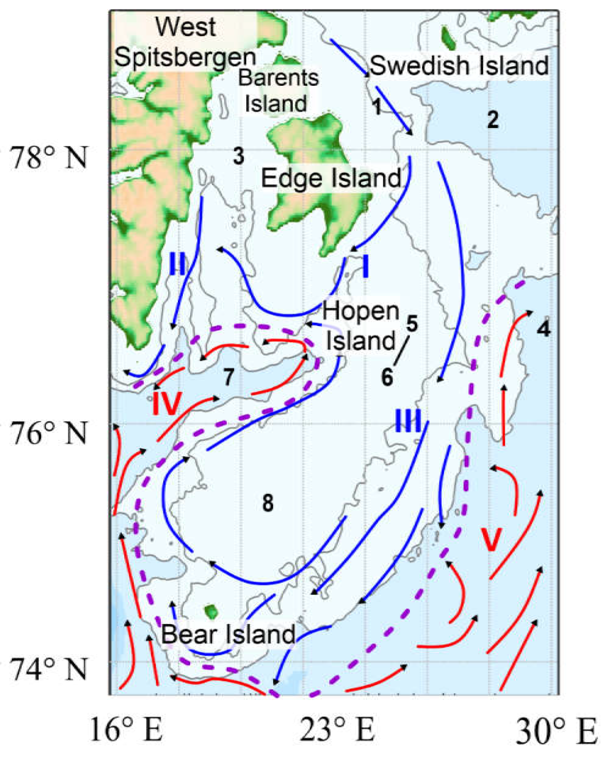
Figure 2.
(a) SAR coverage of the study region from 1 January to 31 December 2018. Black line shows the ice edge position in April 2018. Examples of eddy signatures in SAR images over (b) the open water on 23 August 2018 at 05:50 UTC and (c) the MIZ on 12 February 2018 at 05:50 UTC.
Figure 2.
(a) SAR coverage of the study region from 1 January to 31 December 2018. Black line shows the ice edge position in April 2018. Examples of eddy signatures in SAR images over (b) the open water on 23 August 2018 at 05:50 UTC and (c) the MIZ on 12 February 2018 at 05:50 UTC.
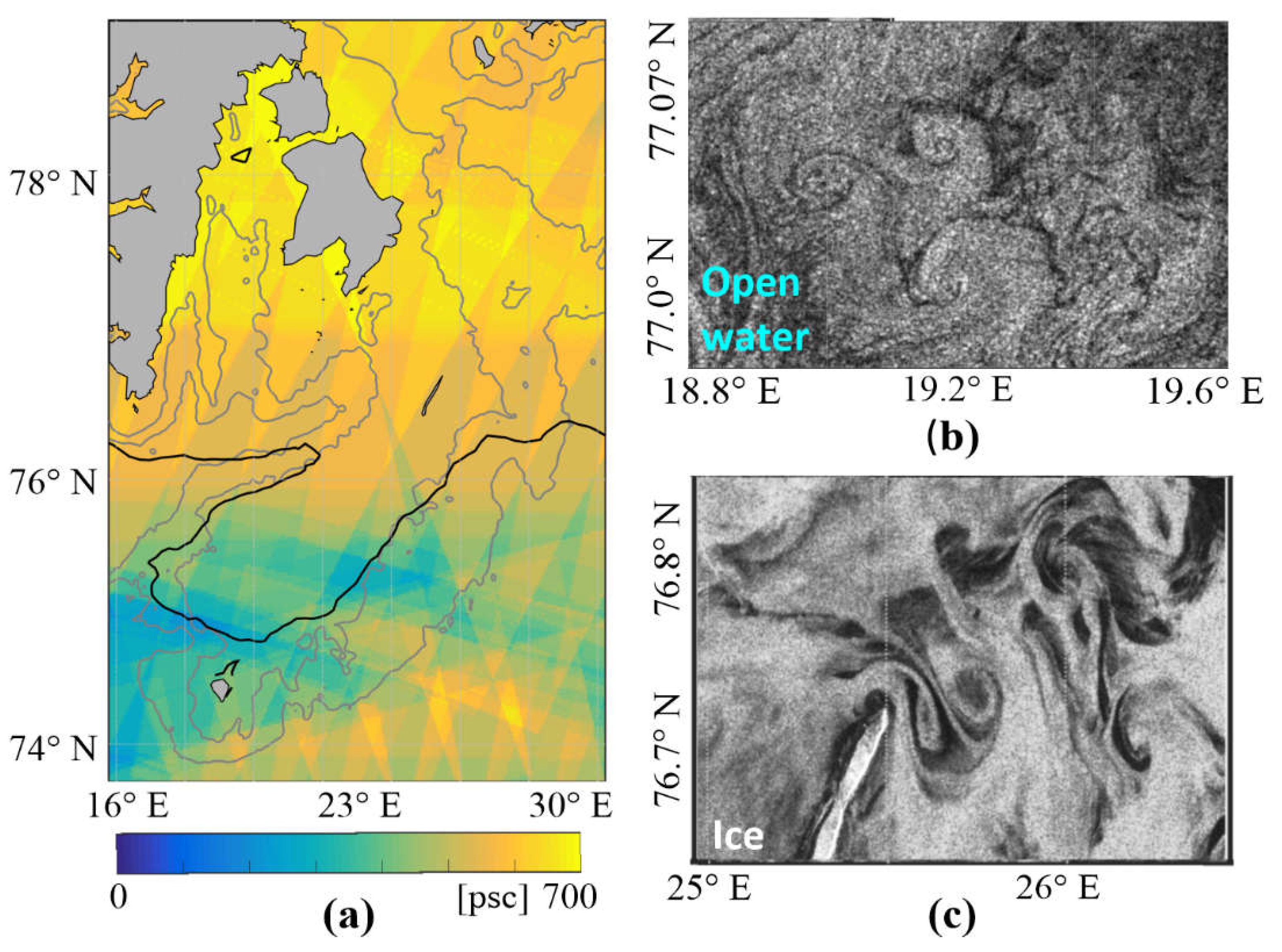
Figure 3.
Spatial distribution of eddy numbers (a), their probability (b) and the mean eddy diameters (c) over the SB. Overlaid grey lines are the 100- and 200-m isobaths.
Figure 3.
Spatial distribution of eddy numbers (a), their probability (b) and the mean eddy diameters (c) over the SB. Overlaid grey lines are the 100- and 200-m isobaths.
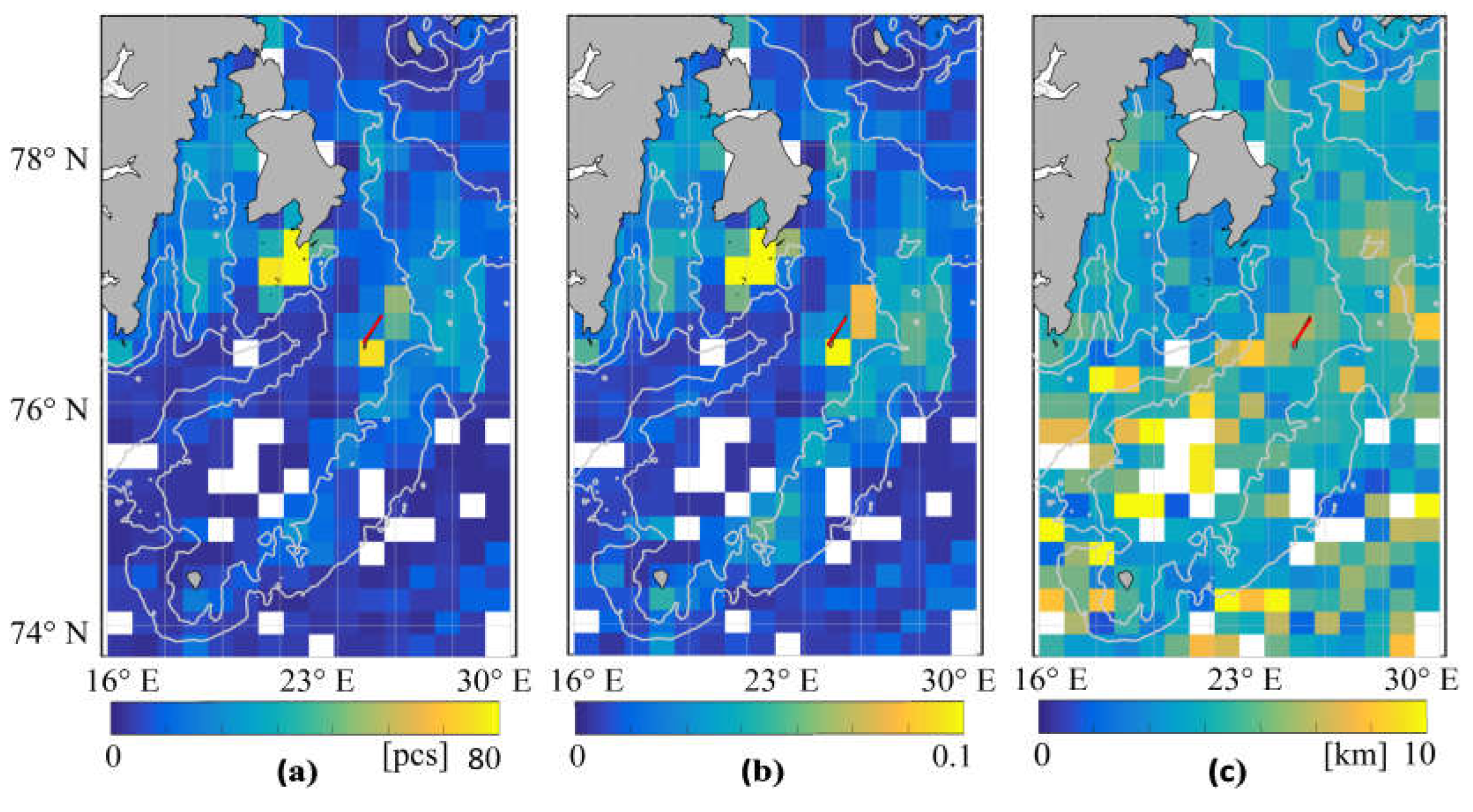
Figure 4.
Spatial distribution of eddy numbers (a-d) and their probability (e-h) during first (a), second (b), third (с) and fourth (d) quarters of 2018. Dotted grey lines are the 100- and 200-m isobaths. Color lines are monthly positions of the ice edge: (a) red line - January, light green – February, magenta – March; (b) orange – April, cyan – May, yellow – June; (f) grey line - December.
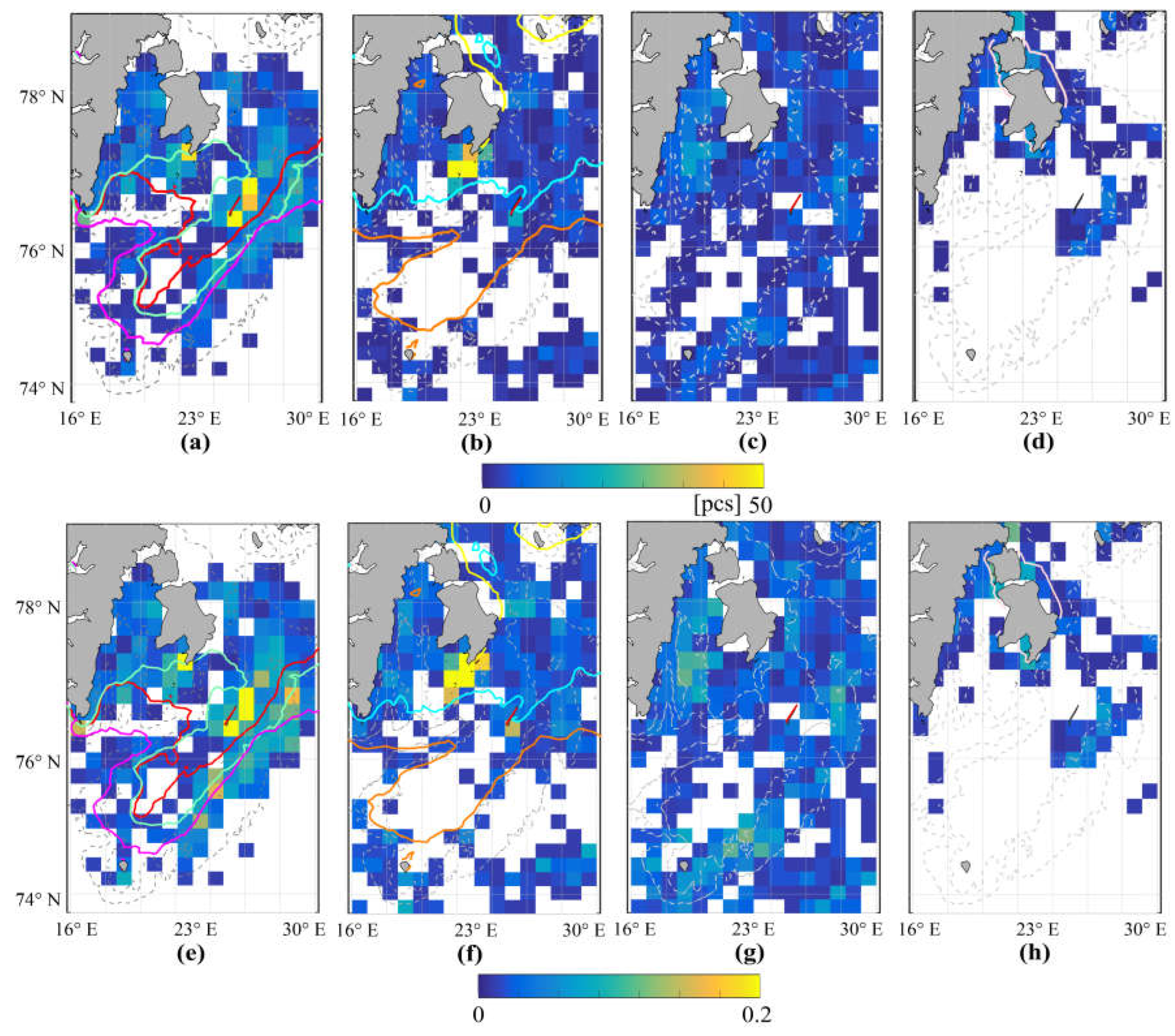
Figure 5.
Monthly distributions of the number of detected eddies (columns) and their monthly-mean diameter values (lines). Dark (light) grey colors correspond to the MIZ (OW) eddies, respectively.
Figure 5.
Monthly distributions of the number of detected eddies (columns) and their monthly-mean diameter values (lines). Dark (light) grey colors correspond to the MIZ (OW) eddies, respectively.
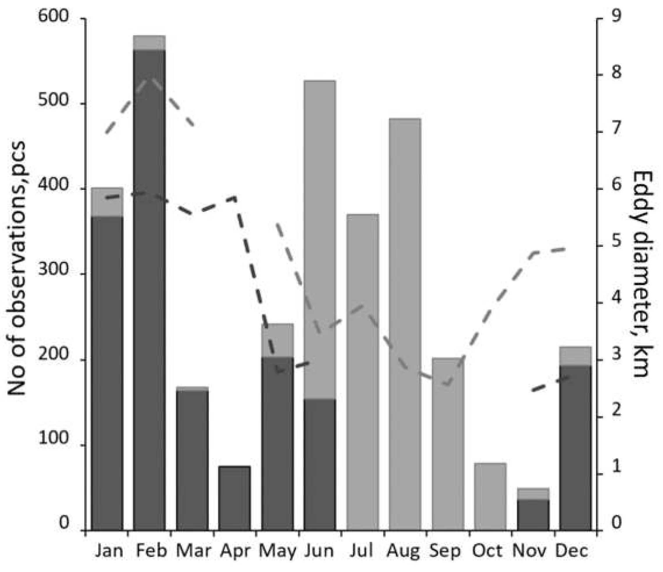
Figure 6.
Locations (a), probability of eddy occurrence (b) and maximum diameters (c) of the MIZ eddies identified in spaceborne SAR data in 2018. Red line marks HI.
Figure 6.
Locations (a), probability of eddy occurrence (b) and maximum diameters (c) of the MIZ eddies identified in spaceborne SAR data in 2018. Red line marks HI.

Figure 7.
Histogram distributions of (a) the number of MIZ eddies as a function of their diameters and (b) monthly variations of the normalized number of MIZ eddies. Black and white colors in (a) correspond to C and AC eddies, respectively. Blue line in (b) is a ratio of C and AC eddies.
Figure 7.
Histogram distributions of (a) the number of MIZ eddies as a function of their diameters and (b) monthly variations of the normalized number of MIZ eddies. Black and white colors in (a) correspond to C and AC eddies, respectively. Blue line in (b) is a ratio of C and AC eddies.
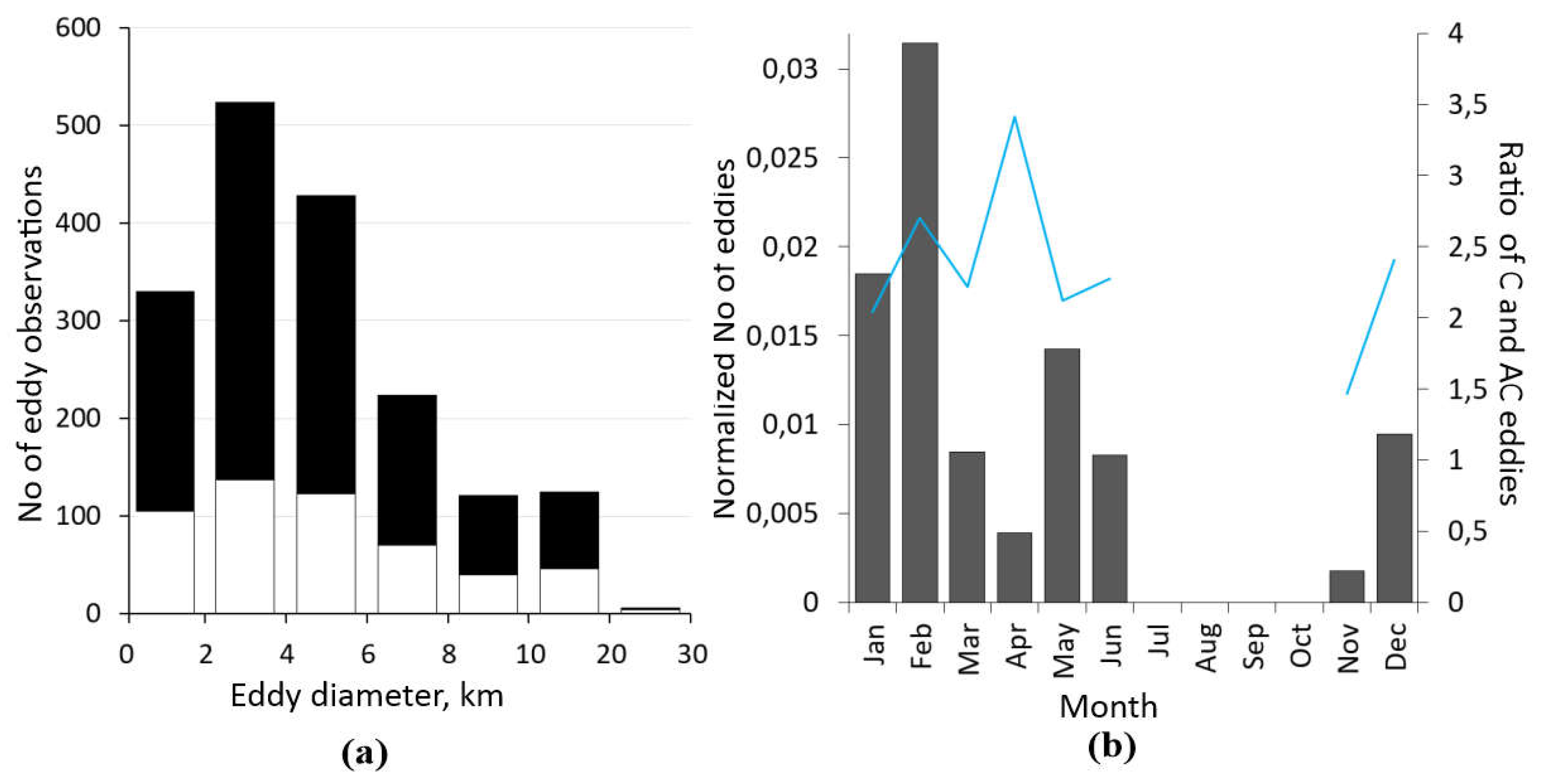
Figure 8.
Maps of normalized radar cross section showing examples of MIZ eddy manifestations in a sequence of Sentinel-1 SAR images acquired on (a) 11 February 2018 at 05:59 UTC, (b) 12 February 2018 at 05:01 UTC, (c) 12 February 2018 at 05:50 UTC, (d) 13 February 2018 at 05:42 UTC near HI.
Figure 8.
Maps of normalized radar cross section showing examples of MIZ eddy manifestations in a sequence of Sentinel-1 SAR images acquired on (a) 11 February 2018 at 05:59 UTC, (b) 12 February 2018 at 05:01 UTC, (c) 12 February 2018 at 05:50 UTC, (d) 13 February 2018 at 05:42 UTC near HI.
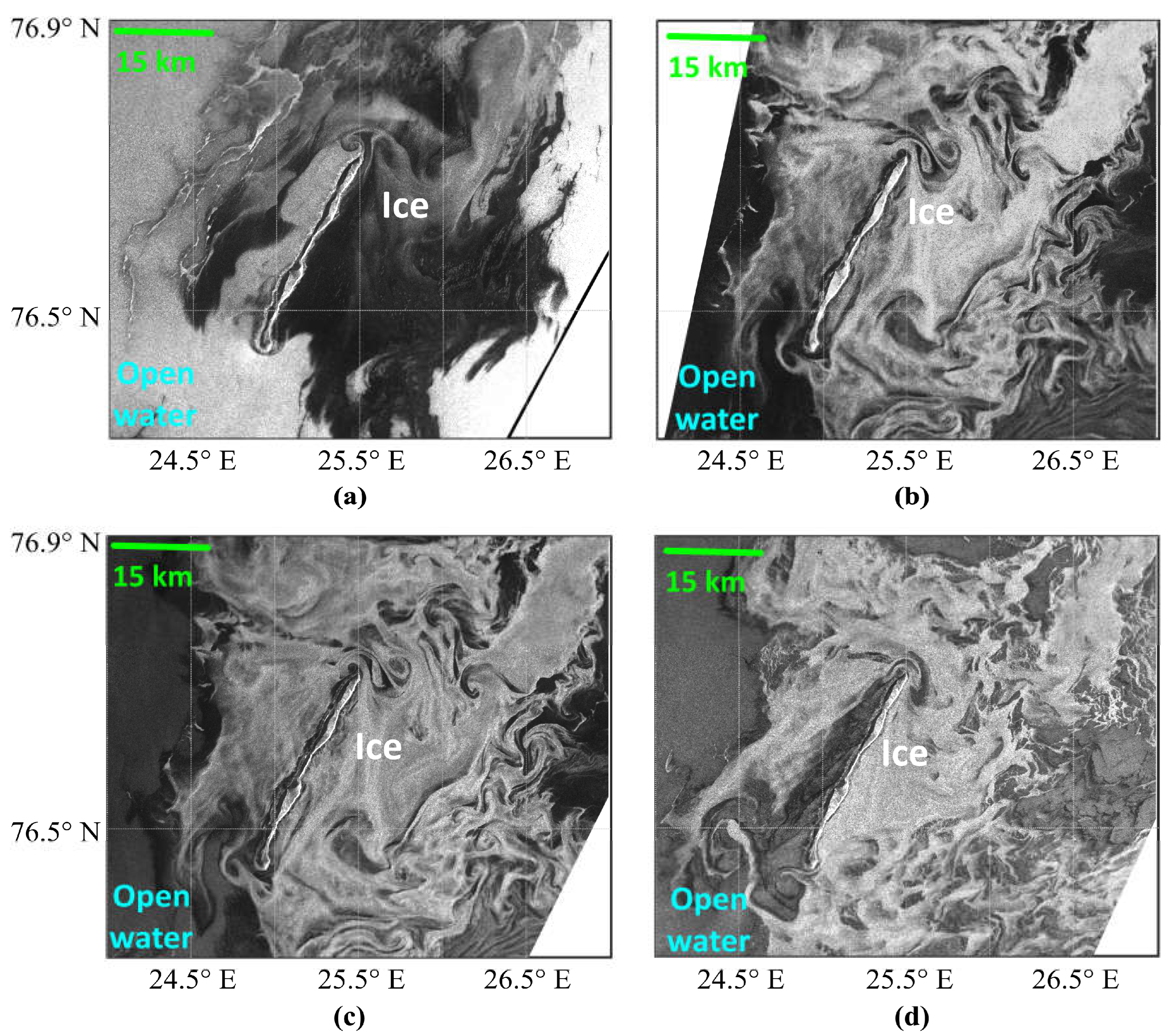
Figure 9.
Locations (a), probability (b) and maximum diameters (с) of OW eddies identified in spaceborne SAR data in 2018.
Figure 9.
Locations (a), probability (b) and maximum diameters (с) of OW eddies identified in spaceborne SAR data in 2018.
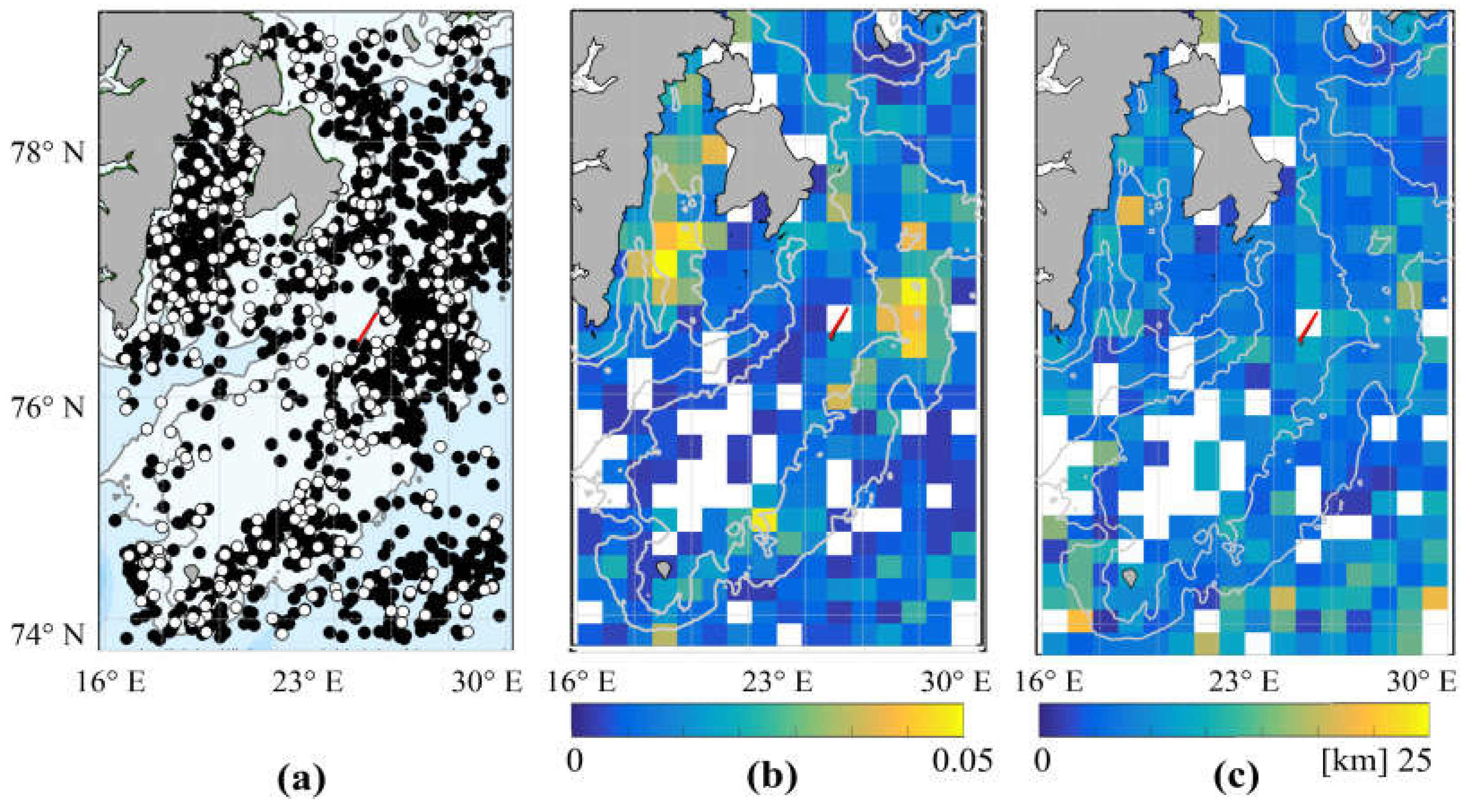
Figure 10.
Histogram distributions of the number of OW eddies as a function of depth (a) and dimensionless slope (b), values corresponding to the location of eddy centers.
Figure 10.
Histogram distributions of the number of OW eddies as a function of depth (a) and dimensionless slope (b), values corresponding to the location of eddy centers.
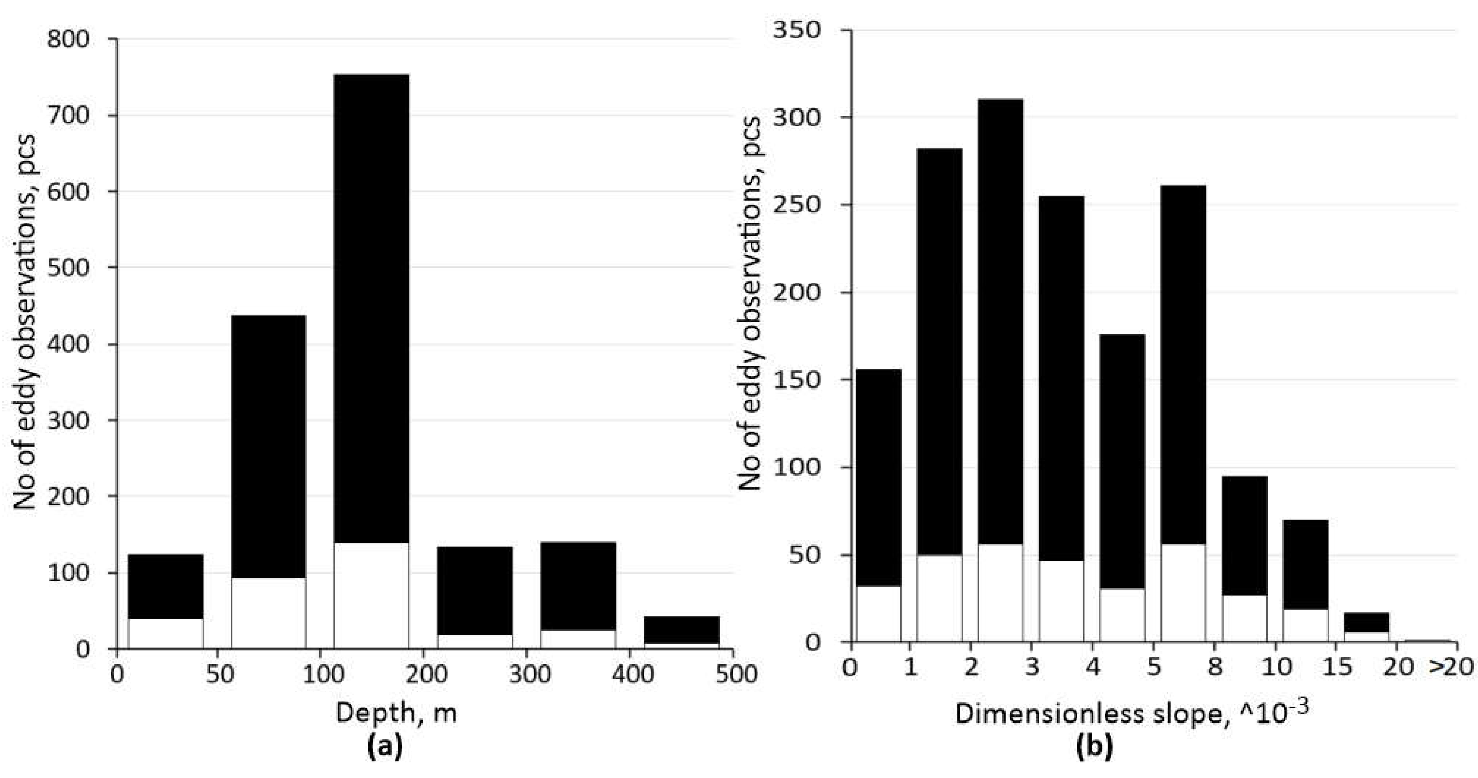
Figure 11.
Histogram distributions of (a) the number of OW eddies as a function of their diameters and (b) monthly normalized number of eddies. Black and white colors in (a) correspond to C and AC, respectively. Blue line on (b) is a ratio of C and AC eddies.
Figure 11.
Histogram distributions of (a) the number of OW eddies as a function of their diameters and (b) monthly normalized number of eddies. Black and white colors in (a) correspond to C and AC, respectively. Blue line on (b) is a ratio of C and AC eddies.
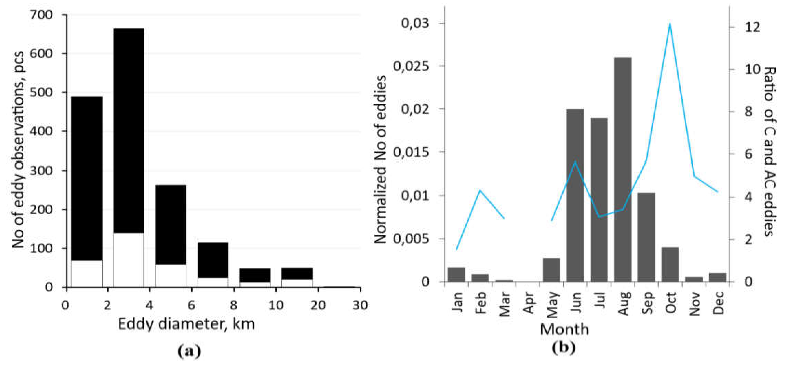
Figure 12.
Spatial fields of dimensionless slope (a), surface current speed (b), near-surface wind speed (c) and SST gradient (d) for August 2018. Magenta circles show locations of eddies registered in SAR data in August 2018. White lines in (d) mark the boundaries of Polar Front.
Figure 12.
Spatial fields of dimensionless slope (a), surface current speed (b), near-surface wind speed (c) and SST gradient (d) for August 2018. Magenta circles show locations of eddies registered in SAR data in August 2018. White lines in (d) mark the boundaries of Polar Front.
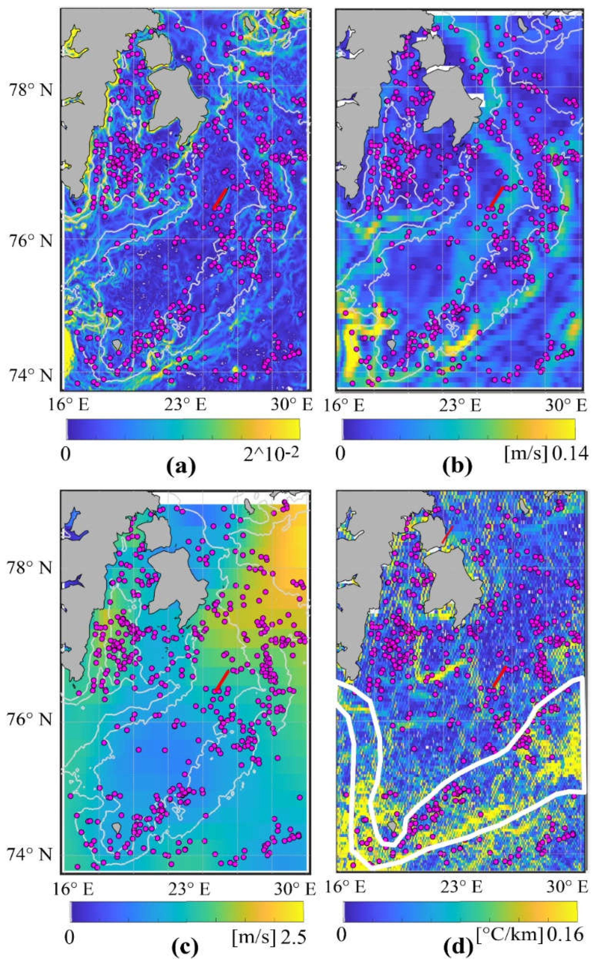
Figure 13.
Schematic depicting main eddy generation mechanisms over the Spitsbergen Bank in the northwestern Barents Sea owing to (a) interaction of currents with sloping bottom, (b) island wakes, (c) frontal generation, (d) dynamic processes in the MIZ. Magenta and green markers in (a) represent cyclones and anticyclones.
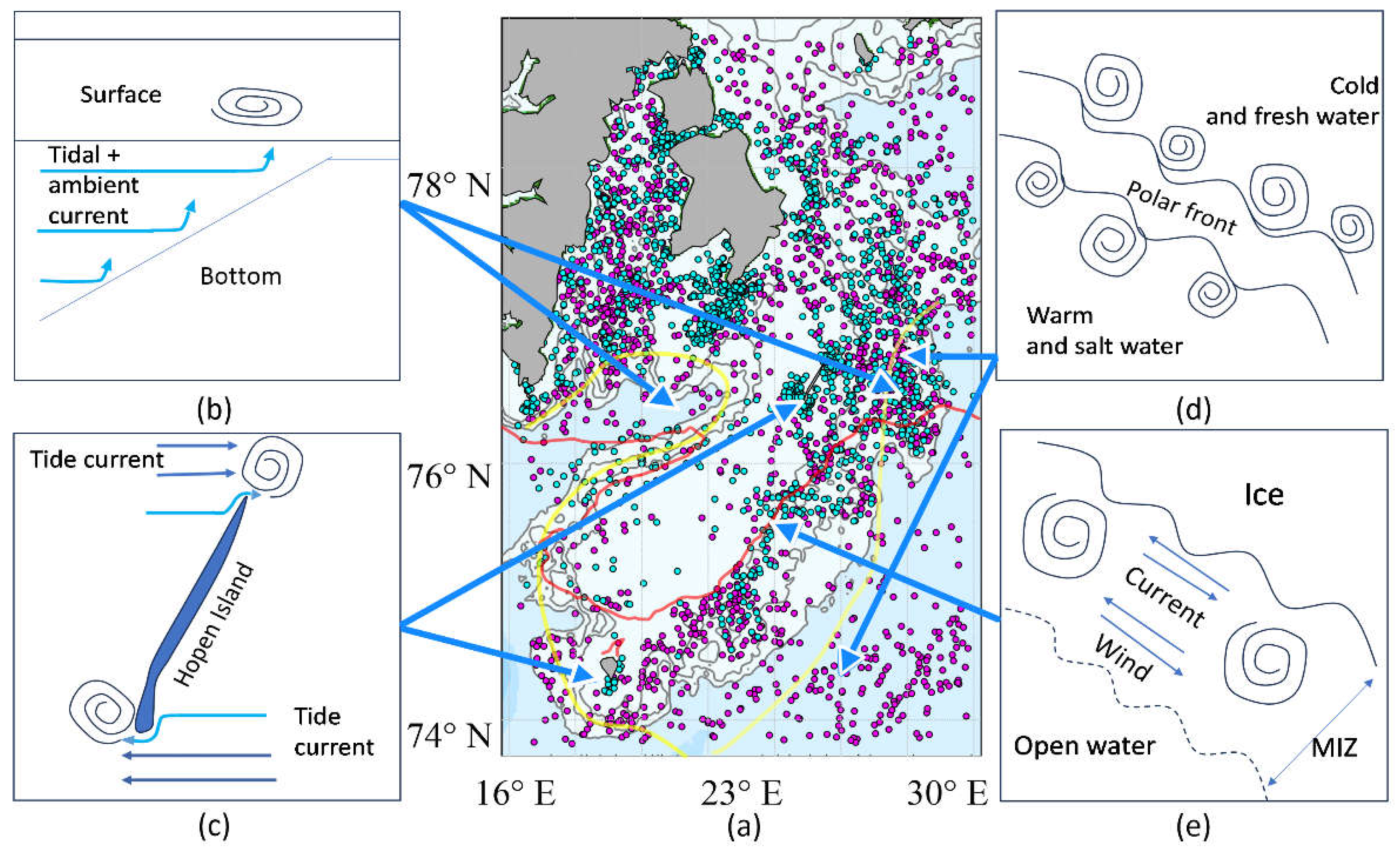

Table 1.
Summary of the MIZ and the OW eddy detection in spaceborne SAR data in quarters of 2018.
| Quarter (Months) | Number of Eddies | Mean Diameter, km |
||
|---|---|---|---|---|
| MIZ | OW | MIZ | OW | |
| 1 (Jan-Mar) | 1095 | 53 | 5.8 | 7.3 |
| 2 (Apr-Jun) | 432 | 412 | 3.4 | 3.6 |
| 3 (Jul-Sep) | 0 | 1054 | 0 | 3.2 |
| 4 (Oct-Dec) | 231 | 112 | 2.7 | 4.2 |
| Total | 1758 | 1631 | 4.8 | 3.5 |
Table 2.
Summary of the MIZ eddy detection in spaceborne SAR data in 2018.
| Month | SAR-images, pcs | Number of Eddies | Mean Diameter (min-max), km | ||||
|---|---|---|---|---|---|---|---|
| C | AС | Total | C | AС | All | ||
| Jan | 267 | 247 | 121 | 368 | 5.7 (0.6 - 23.4) | 6.2 (1.1 - 18.7) | 5.9 |
| Feb | 244 | 411 | 152 | 563 | 5.7(1.4 - 39.3) | 6.7 (1.4 - 27.9) | 5.9 |
| Mar | 266 | 113 | 51 | 164 | 5.6 (0.9 - 18) | 5.4 (1.1 - 11.9) | 5.6 |
| Apr | 261 | 58 | 17 | 75 | 5.9 (1.3 - 15.2) | 5.7 (1.5 - 9.3) | 5.8 |
| May | 180 | 138 | 65 | 203 | 2.8 (0.4 - 8.9) | 2.8 (0.7 - 9.5) | 2.8 |
| Jun | 255 | 107 | 47 | 154 | 2.8 (0.5 - 11.2) | 3.5 (0.8 - 11.7) | 3.0 |
| Jul | 264 | - | - | - | - | - | - |
| Aug | 251 | - | - | - | - | - | - |
| Sep | 255 | - | - | - | - | - | - |
| Oct | 268 | - | - | - | - | - | - |
| Nov | 281 | 22 | 15 | 37 | 2.3 (0.9 - 4.9) | 2.7 (0.6 - 8) | 2.5 |
| Dec | 278 | 137 | 57 | 194 | 2.8 (0.2 - 8.6) | 2.6 (0.4 - 10.1) | 2.8 |
| Total | 3070 | 1233 | 525 | 1758 | 4.7 | 5.1 | 4.8 |
Table 3.
Summary of the open water eddy detection in spaceborne SAR data in 2018.
| Month | SAR-images, pcs | Number of Eddies | Mean Diameter (min-max), km | ||||
|---|---|---|---|---|---|---|---|
| C | AС | Total | C | AС | All | ||
| Jan | 267 | 20 | 13 | 33 | 7.6 (3 - 16.4) | 6.1 (2.4 - 13.8) | 7.0 |
| Feb | 244 | 13 | 3 | 16 | 7 (2.9 - 13.7) | 12.2 (9.2 - 15.1) | 8.0 |
| Mar | 266 | 3 | 1 | 4 | 8.8 (6.6 - 10.9) | 2.0 | 7.1 |
| Apr | 261 | ||||||
| May | 180 | 29 | 10 | 39 | 5.8 (1.3 - 14.9) | 4.1 (1.4 - 9.5) | 5.4 |
| Jun | 255 | 317 | 56 | 373 | 3.5 (0.4 - 12.6) | 3.3 (0.6 - 7.8) | 3.5 |
| Jul | 264 | 279 | 91 | 370 | 3.6 (0.6 - 21) | 4.9 (1.1 - 14.5) | 4.0 |
| Aug | 251 | 373 | 109 | 482 | 2.7 (0.5 - 20) | 3.5 (0.7 - 18.4) | 2.9 |
| Sep | 255 | 172 | 30 | 202 | 2.5 (0.6 - 10.6) | 2.8 (0.6 - 10) | 2.6 |
| Oct | 268 | 73 | 6 | 79 | 3.7 (1.1 - 9.5) | 5.6 (2.9 - 10.6) | 3.9 |
| Nov | 281 | 10 | 2 | 12 | 4.3 (1.8 - 7.8) | 7.8 (3.9 - 11.7) | 4.9 |
| Dec | 278 | 17 | 4 | 21 | 4.8 (0.7 - 17) | 5.6 (0.8 - 19.7) | 5.0 |
| Total | 3070 | 1306 | 325 | 1631 | 3.4 | 4.1 | 3.5 |
Disclaimer/Publisher’s Note: The statements, opinions and data contained in all publications are solely those of the individual author(s) and contributor(s) and not of MDPI and/or the editor(s). MDPI and/or the editor(s) disclaim responsibility for any injury to people or property resulting from any ideas, methods, instructions or products referred to in the content. |
© 2024 by the authors. Licensee MDPI, Basel, Switzerland. This article is an open access article distributed under the terms and conditions of the Creative Commons Attribution (CC BY) license (http://creativecommons.org/licenses/by/4.0/).
Copyright: This open access article is published under a Creative Commons CC BY 4.0 license, which permit the free download, distribution, and reuse, provided that the author and preprint are cited in any reuse.


