Indirect Model Predictive Control on Epidemiological Stochastic Blockmodels

Preprint

Article

Indirect Model Predictive Control on Epidemiological Stochastic Blockmodels

Altmetrics

Downloads

Views

Comments

This version is not peer-reviewed

Submitted:

02 May 2024

Posted:

06 May 2024

You are already at the latest version

Alerts

Abstract

This paper aims to demonstrate how the detection of communities for epidemiological networks can be used to reduce the dimensionality of optimal control problems. A range of planted partition stochastic blockmodels are generated, where the underlying communities in the model vary in detectability. A high-performance computing workflow is then used to simulate and estimate reduced model dynamics for the networks, which in turn is used to find optimal control solutions.

Keywords:

Subject: Engineering - Control and Systems Engineering

1. Introduction

1.1. Background

Ranking as one of the deadliest epidemics in history [1], the The COVID-19 pandemic has shown the need for accuracy in the modeling and response to epidemics. In order to mitigate the spread of such diseases, it is important to develop models that are able to utilize all data available that can be used to determine the epidemics course.

Epidemics on large populations are usually modeled with compartmental models like the Kermack-McKendrick (SIR) model [2] which models disease infection and recovery. These models yield accurate predictions for homogenous populations.

In contrast to these frequently used compartmental models, the true dynamics of an epidemic is heterogenous and exhibits the small-world and scale-free properties exhibited by real-world networks [3]. Network dataset analysis on mobile communication records and mobility fluxes [4] shows strong correlations between mobility and communitation patterns in populations, which encourages usage of heterogenous epidemiological network models. These models also enable data association on more detailed levels, which enables the implications of targeted control inputs (such as disease spread mitigation strategies, self-quarantine recommendations and local restrictions on facilities and events) to be compared to implications of more global control strategies (such as regional lockdowns and restrictions on large population gatherings).

Model predictive control on compartmental models is generally computationally feasible, both for nonlinear programs (NLPs) and mixed-integer ones. In contrast, due to the number of distinct control inputs that can be present in an epidemiological network model, direct optimization on the network model is not computationally feasible. A remedy for this issue is to approximate parts of these networks with simpler models, and instead solve control problems for these approximations. These approximations needs to account both for the underlying graph structure and the dynamics of the network.

Extensive work has previously been done on the approximation of graph structures, and it is frequently used for community detection and cluster identification in networks. Bayesian inference methods are usually applied to networks, in order to categorize nodes into distinct partions. Stochastic blockmodels (SBMs) are generally used to retrieve partitions that capture clusters and communities, which can be used to form hierarchical layers of graphs [5]. The majority of theory related to SBM-inference in this paper is summarized in [6]. This includes the detectability-indetectability phase transition, which is used to demonstrate how control input dimensionalities can be reduced when the number of detected communities are reduced.

One potential solution to avoid the infeasibility of graph optimization is to treat network models as black-box models, which only considers input signals and output measurements of the network. Black-box models lack interpretability and transparency, which are important properties for control strategies that potentially have fatal consequences. A remedy for the interpretability in black-box models is sparse nonlinear regression methods, which have gained traction over the recent years [7]. Sparse nonlinear regression enable the identification of models based on input signals and output measurements, such that the resulting models consists of as few parameters as possible.

Monte Carlo (MC) methods are used with Bayesian inference in order to approximate posterior distributions for the quantities of Susceptible (S), Infectious (I) and Recovered (R) individuals in the networks populations. Importance sampling [8] is frequently used to reduce the dimensionality of the sample space, which in this paper is used on the stochastic dynamics found in the edges of dynamical networks.

1.2. Overview

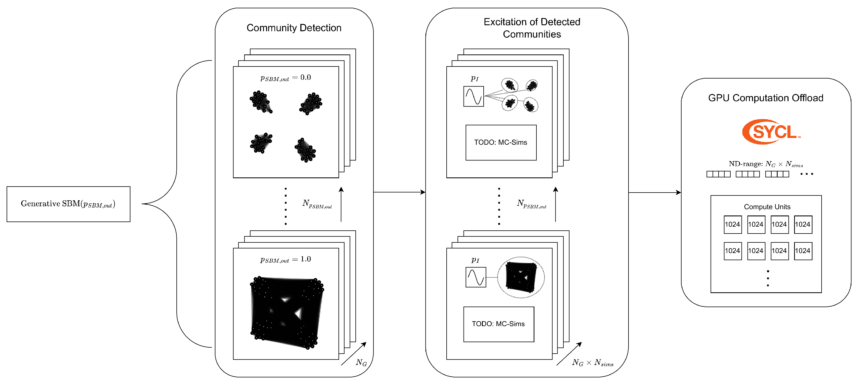
This paper presents a high performance computing (HPC) workflow for simulation, model reduction and optimal control of epidemics, from the level of an individual-based network model. The workflow is demonstrated by performing MC-simulations, community detection, regression and optimal control over networks whose population clusters become increasingly more interconnected (Figure 1). The relation between them will be explained by first introducing the community and individual level dynamics, followed by a bayesian inference approach to identify communities for weighted graphs.

MC-simulations are run on the identified communities, which generates data used to fit Least Squares (LS) and Quantile Regression (QR) models. These models are then used to approximate Robust Model Predictive Control (RMPC) problems aimed at minimizing the total number infected of an epidemic with minimal intervention. Finally, the control input solutions are validated with new MC-simulations on the networks.

2. Epidemiological Models

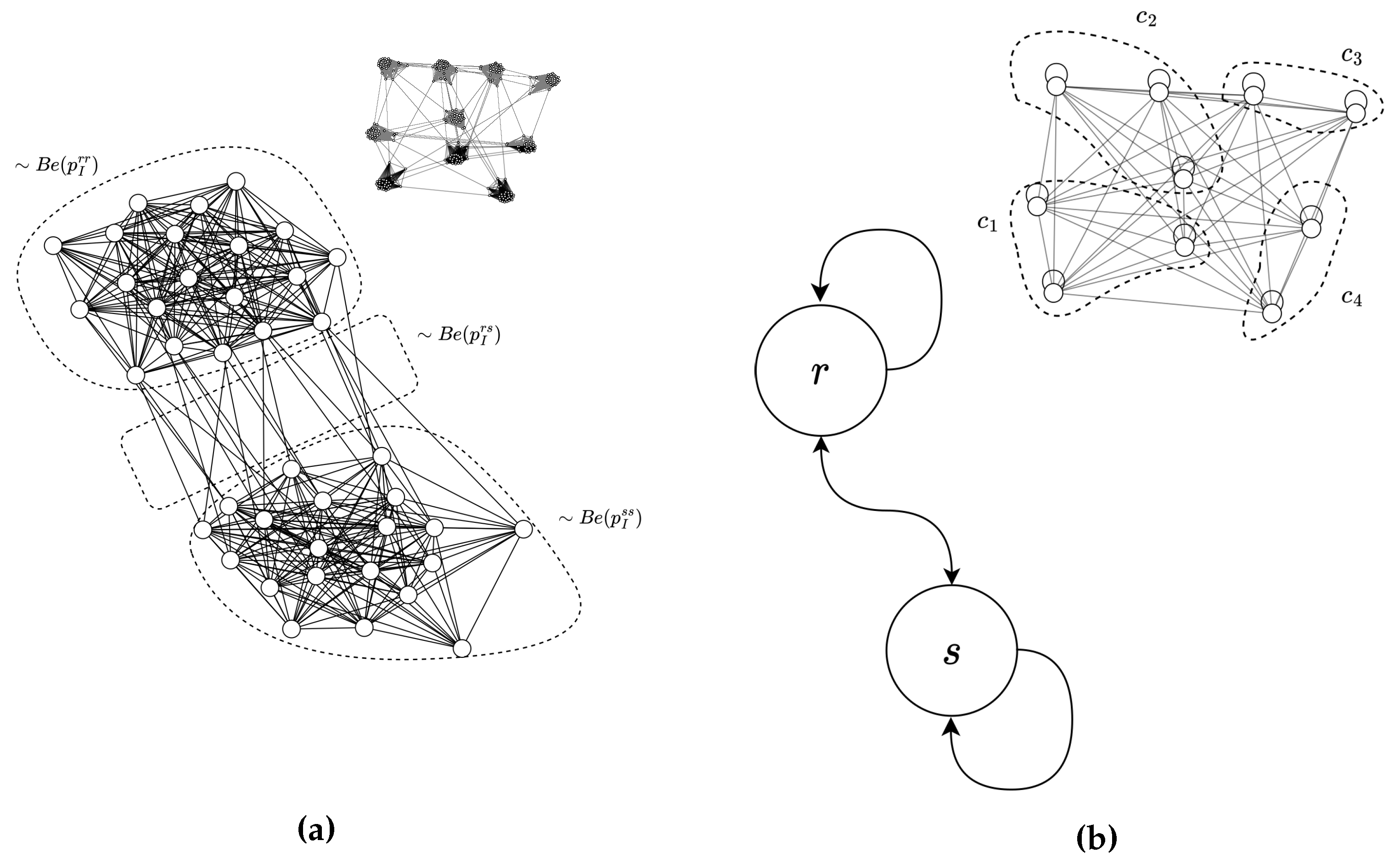
This paper utilize three levels of graph-structured epidemiological models, which are all described by separate adjacency matrices (individual-level

A_{S B M}

, partition-level

A_{p a r t}

and community-level

A_{c o m}

). The next sections formulate dynamics for the individual and community levels.

2.1. Community SIR Model

A community SIR model can be defined for a population in order to account for infections caused by external populations. Compartmental populations

N_{S}, N_{I}

and

N_{R}

denote the susceptible, infected and recovered groups of each community.

Individuals are divided into communities

c = {c_{1}, \dots, c_{N_{c}}}

, where n and m denotes source and target communities. Infections inside (

n = n

) and between communities occur over discrete timesteps t with bilinear infection dynamics.

Δ N_{I, t}^{(r s)} = θ_{r s} \frac{N_{S, t}^{(r)} N_{I, t}^{(s)}}{N_{S, t}^{(s)} + N_{I, t}^{(r)} + N_{R, t}^{(s)}}

(1)

θ = [θ_{11}, θ_{12}, \dots, θ_{N_{c} N_{c}}]

contains parameters the average number of contacts between communities for each person over a timestep. A known recovery rate

α

applies to all infected individuals, which in combination with (1) can be used to derive discrete dynamics (2-4) for the health states of all communities.

\begin{matrix} Δ N_{S, t}^{(r)} & = - \sum_{s \in c} Δ N_{I, t}^{(r s)} \end{matrix}

(2)

\begin{matrix} Δ N_{I, t}^{(r)} & = \sum_{s \in c} Δ N_{I, t}^{(r s)} - α N_{I, t}^{(r)} \end{matrix}

(3)

\begin{matrix} Δ N_{R, t}^{(r)} & = α N_{I, t}^{(r)} \end{matrix}

(4)

2.2. Stochastic Blockmodel

Let

b

denote vertex partitions in the individual-level graph with adacency matrix

A_{S B M}

. The stochastic blockmodel is a generative graph model parameterized by a probabilities

p_{S B M}

, where

p_{S B M, r s}

denotes the probability of generating an edge between vertices contained in partitions r and s. From a Bayesian perspective,

p_{S B M}

parameterize the maximum entropy probability distribution for generating an adjacency matrix

A_{S B M}

over partitions

b

[6]. Graphs generated in this paper utilize the planted partition SBM, which is parameterized by internal probability

p_{S B M, i n}

(for

r = s

), and outgoing probability

p_{S B M, o u t}

. It should be emphasized that this papers graphs are static, in contrast to dynamic contact networks.

2.3. Stochastic SIR Network Model

Each vertex

v_{i} \in {0, \dots N_{V} - 1}

is assigned a state

V_{i} (t) \in {S = 0, I = 1, R = 2}

. Initial infections are assigned with Bernoulli probability

p_{I, 0}

, with remaining individuals initially assigned as susceptible. Edges between vertices of partitions r and s are assigned uniform infection probability

p_{I}^{(r s)}

q_{r, t}^{(i)}

is used to denote the number infectious contact events inflicted upon an individual

v_{i}

by partition r.

q_{r, t}^{(i)} (ω) = \sum_{j \in N_{I, t}^{(i, r)}} q_{I, t}^{(i j)} (ω) \sim B i n (N_{I, t}^{(r)}, p_{I}^{(r b (i))})

(5)

For each sample

ω

from the full space of possible outcomes

Ω

q_{I, t}^{(i j)} (ω) \sim B e (p_{I}^{(r s)})

are contact events occuring between communities at time t, and

q_{R, t}^{(i)} (ω) \sim B e (p_{R})

are recovery events.

N_{I, t}^{(i, r)}

denotes the infected neighborhood of

v_{i}

located in r. Since infections between partitions are uniformly Bernoulli-distributed, the resulting number of community contact events inflicted on an individual are binomially distributed.

Under Markov assumptions, the dynamics for an individual

V^{(i)}

can be formulated.

V_{t + 1}^{(i)} = \{\begin{matrix} 1 (\sum_{r \in b} q_{r, t}^{(i)} (ω)), & V_{t}^{(i)} = S \\ 1 + q_{R, t}^{(i)} (ω), & V_{t}^{(i)} = I \end{matrix}

(6)

The purpose of the detailed notation is to obtain infection likelihoods between all communities. The likelihood for an individual to be infected by a community is determined by the infection event contributions from all communities.

L_{r} (V_{t + 1}^{(i)} = I) = \frac{q_{r, t}^{(i)} (ω)}{\sum_{s \in c} q_{s, t}^{(i)} (ω)}

(7)

Since an individual can be exposed to multiple contact events during a timestep, the likelihood will be used to sample the events that actually cause the infections.

3. Weighted Graph Bayesian Inference

Structural inference will be performed on the partition-level (

A_{p a r t}

), where partitions

b

labels individuals that are subject to common control inputs (Figure 2). Probability for generating an adjacency matrix

A

over communities

c

is given as [6]:

\begin{matrix} P (A | λ, c) = & \prod_{n < m} \frac{e^{- λ_{c_{n}, c_{m}}} λ_{c_{n}, c_{m}}^{A_{n m}}}{A_{n m}!} \\ \times & \prod_{i} \frac{e^{- λ_{c_{n}, c_{m}} / 2} {(λ_{c_{n}, c_{m}} / 2)}^{A_{n n} / 2}}{(A_{n n} / 2)!} \end{matrix}

(8)

Where

λ_{n m}

is the average number of edges between pairs of nodes in communities

n, m

Decoupling the inference of dynamics and structure can be challenging for arbitrary dynamical networks. Due to uniform assignments of

p_{I}

, this paper assumes that all edges are equally important for the structural inference problem, which makes it possible to decouple the inference of communities from the inference of parameters for the community ODE. With prior distribution

P (c)

the posterior distribution for

c

becomes:

P (c | A) = \frac{\int P (A | λ, c) P (λ | c) d λ P (c)}{P (A)}

(9)

4. Monte-Carlo Importance Sampling

In order to relate the stochastic network model (6) to the deterministic one (2-4) Monte-Carlo (MC) importance sampling will be used to approximate marginal likelihoods for the communities. Let

p_{I, t}^{(r s)} \sim U (p_{I, m i n}, p_{I, m a x})

ξ

denote the vector of all random variables

U_{I, 0 : N_{t}}, U_{R, 0 : N_{t}}, p_{I, 0 : N_{t} - 1}

in the network models trajectory, and let

θ_{G} = {G_{S B M}, p_{I, 0}, p_{R}}

denote all fixed parameters required for initialization of the network.

Community-level dynamics can be captured by measuring infections between and recoveries inside of the network communities.

\begin{matrix} y_{I, t} & = [Δ N_{I, t}^{(11)}, Δ N_{I, t}^{(12)}, \dots, Δ N_{I, t}^{(N_{c} N_{c})}] \end{matrix}

(10)

With

y_{I, 0 : N_{t} - 1}

y \in Z^{N_{t} \times (\binom{N_{c}}{2})}

, the marginal distributions for the full network trajectory can be found by integrating over

ξ

p (y | θ_{G}) = \int_{ξ} p (y, ξ | θ_{G}) p (ξ) d ξ

(11)

Variance of the MC-simulations are reduced by advancing the network dynamics with (6), which amounts to importance distribution

π (.)

I = \int_{y} p (y | θ_{G}) π (y | θ_{G}) d y

(12)

Statistical moments of interest I can be approximated by drawing samples of

{y^{(k)}}_{k = 1}^{N_{M C}}

from

π (.)

, where

N_{M C}

denotes the total number of MC-simulations. The regression performed in this paper will approximate expected and ’worst-case’ number of infections between and inside each community.

\begin{matrix} E_{N} (y | θ_{G}) & = \sum_{k = 0}^{N_{M C} - 1} y^{(k)} p (y^{(k)} | θ_{G}) \end{matrix}

(13)

\begin{matrix} P_{N} (y \leq y_{I, τ} | θ_{G}) & = \sum_{y \leq y_{I, τ}} p (y^{(k)} | θ_{G}) \end{matrix}

(14)

y_{I, τ}

denotes the conditional median number of infected for

y

, given quantile

τ

. In order to avoid an overrepresentation of endemic states (and degeneracy in the regression problem) MC-simulations are terminated early whenever

N_{I, t} < N_{I, m i n}

Bounds for

p_{I}

are retrieved from the reproduction number

R_{0}

of the SBM.

p_{I} = 1 - e^{\frac{log 1 - p_{R} R_{0}}{〈 k 〉}}

(15)

Where

〈 k 〉

is the expected degree for the vertices.

5. Regression

5.1. Regression Model

The regression algorithm aims to identify the bilinear dynamics found in (3), which is achieved by transforming MC-data to the same form.

\begin{matrix} F_{θ_{r s}} (x_{t}^{(r)}, x_{t}^{(s)}, p_{I, t}^{(r s)}) & = p_{I, t}^{(r s)} θ_{r s} \frac{N_{S, t}^{(s)} N_{I, t}^{(r)}}{N_{S, t}^{(s)} + N_{I, t}^{(r)} + N_{R, t}^{(s)}} \end{matrix}

(16)

F_{θ_{r s}}

captures the identified infection dynamic between a single community pair.

5.2. Objective

The regression objectives aims to find good estimators for (13) and (14). For the infection dynamics, this can be decoupled into

(\binom{N_{c}}{2})

regression objectives.

arg min_{{\hat{θ}}_{θ_{r s}}} | | y_{I, M C}^{(r s)} - F_{θ_{r s}} (x_{t}^{(r)}, x_{t}^{(s)}, p_{I, t}^{(r s)}) | |

(17)

(17) is linear, and can be solved using least squares in order to approximate (13) with expected infection rate

{\hat{θ}}_{r s}

. (14) can be approximated with quantile regression, resulting in a linear program (LP).

\begin{matrix} arg min_{θ_{r s, τ}} | | f_{τ} (θ_{r s, τ}, y_{M C}^{(r s)}, x_{M C}^{(r)}, x_{M C}^{(s)}) | | \end{matrix}

(18)

\begin{matrix} f_{τ} (θ_{θ_{r s}, τ}, y_{t}, x_{t}^{(r)}, x_{t}^{(s)}) = \{\begin{matrix} (1 - τ) | F_{θ_{r s}} (x_{t}^{(r)}, x_{t}^{(s)}, p_{I, t}^{(r s)}) | \\ if y_{r} < F_{θ_{r s}} (x_{t}^{(r)}, x_{t}^{(s)}, p_{I, t}^{(r s)}) \\ τ | y_{r} - F_{θ_{r s}} (x_{t}^{(r)}, x_{t}^{(s)}, p_{I, t}^{(r s)}) | \\ else \end{matrix} \end{matrix}

(19)

6. Optimal Control Problem

6.1. Robust Model Predictive Control

\begin{matrix} arg min_{w, u} & Φ (w, u) \end{matrix}

(20)

\begin{matrix} s . t & w_{0} = {\bar{w}}_{0} \end{matrix}

(21)

\begin{matrix} τ & \leq P (g (w_{t}) \leq 0) \forall t ∖ 0 \end{matrix}

(22)

\begin{matrix} p_{I, \min} \leq u_{t} \leq p_{I, \max} \forall t ∖ N_{t} \end{matrix}

(23)

(21-23) presents a robust Optimal Control Problem (OCP) with objective

Φ

, state trajectory

w

and control inputs

u

. Robustness of the OCP is enforced with single chance constraints [9] in (22), which relate probability distributions to the OCP as inequality constraints.

6.2. Regression Model Predictive Control

The OCP for this paper balance the cost of disease spread mitigation against the cost of disease spread. Let

w_{t} \in R^{3 N_{c}}, u_{t} \in R^{2 (\binom{N_{c}}{2}) + N_{c}}

be the compartmental states and control inputs at time t for the OCP. An ordinary differential equation for

w

can be composed from the identified regression models.

\begin{matrix} F_{r} (w_{t}, u_{t}) & = [\begin{matrix} - \sum_{s \in c} F_{r s} (w_{t}^{(r)}, w_{t}^{(s)}, u_{t}^{(r s)}) \\ - \sum_{s \in c} F_{r s} (w_{t}^{(r)}, w_{t}^{(s)}, u_{t}^{(r s)}) + α w_{I, t}^{(0)} \\ α w_{I, t}^{(0)} \end{matrix}] \end{matrix}

(24)

\begin{matrix} F (w_{t}, u_{t}) & = [\begin{matrix} F_{1} (w_{t}, u_{t}) \\ ⋮ \\ F_{N_{c}} (w_{t}, u_{t}) \end{matrix}] \end{matrix}

(25)

With

F

identified, the chance constraint (22) can be approximated.

Φ

can be defined to minimize the number of infected while restricting the usage of the control input, which together is used to formulate the full regression model OCP (26-29)

\begin{matrix} arg min_{w, u} & \sum_{t = 1}^{N_{t}} {\frac{\sum w_{I, t}}{N_{p o p}} - \frac{W_{u}}{N_{p o p}} (u_{t} - u_{\max})} \end{matrix}

(26)

\begin{matrix} s . t & w_{0} = {\bar{w}}_{0} \end{matrix}

(27)

\begin{matrix} w_{t + 1} = F (w_{t}, u_{t} | θ) \forall t ∖ N_{t} \end{matrix}

(28)

\begin{matrix} p_{I, \min} \leq u_{t} \leq p_{I, \max} \forall t ∖ N_{t} \end{matrix}

(29)

7. Simulations

7.1. Structural Inference

In order to demonstrate the control and prediction capabilities of the presented method, a large number of individual-level graphs (

N_{G}

) is generated for the MC-simulations. The partitions are given a population size large enough to be approximated by ODEs, but small enough to give the partitions a considerable variance. The number of partitions (

N_{b}

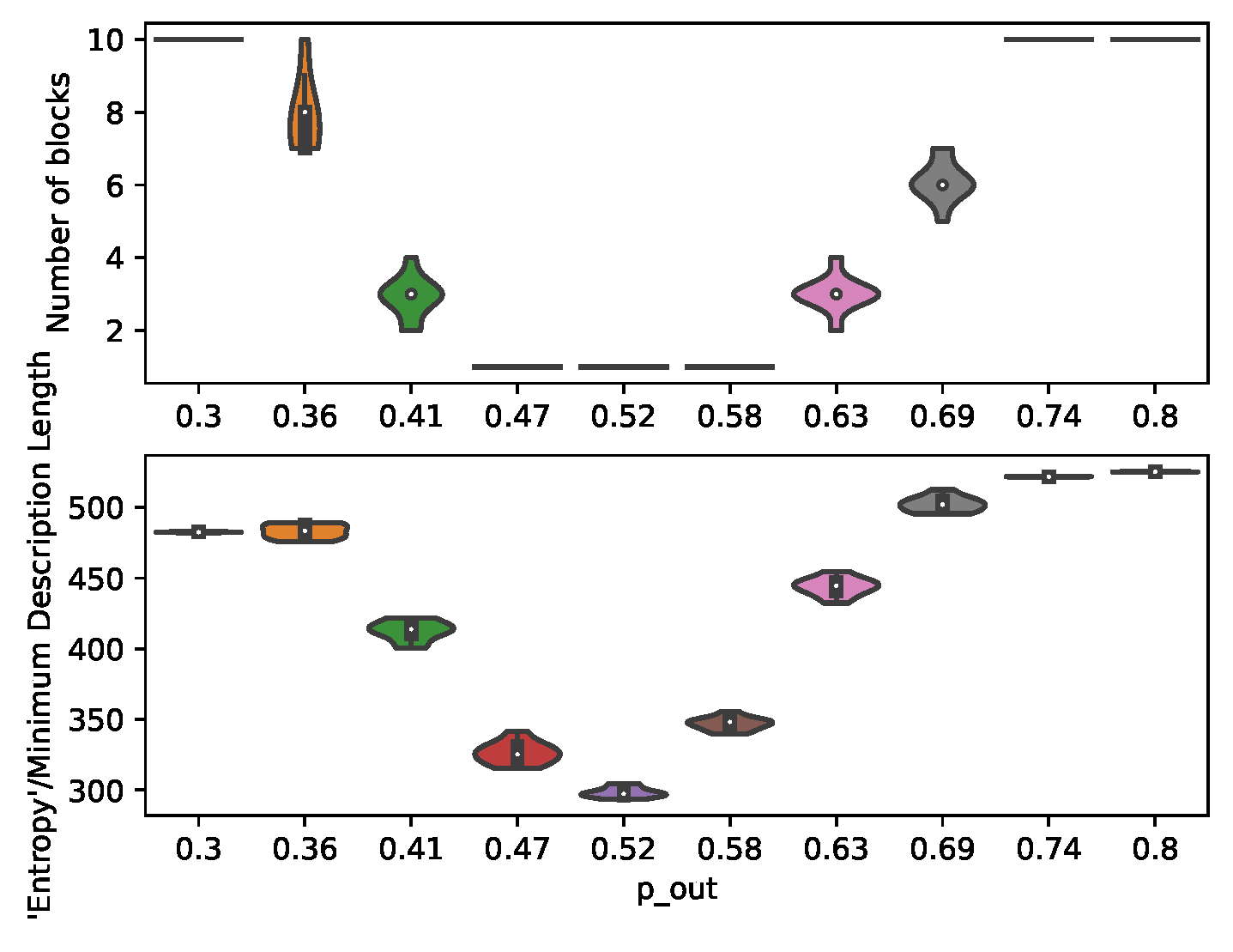
) is set high in order to provide a more granular transition through the community detection threshold (Figure 3).

Figure 3. Inferred number of communities and minimum description length for graphs generated under different

p_{S B M, o u t}

Figure 3. Inferred number of communities and minimum description length for graphs generated under different

p_{S B M, o u t}

Table 1. Graph generation parameters.

$p_{S B M, o u t}$	$[0.3 : 0.05 : 0.8]$	$N_{p o p, b}$	100
$p_{S B M, i n}$	0.5	$N_{G}$	100
$N_{b}$	10

Estimates for (9) are computed using an importance sampling algorithm [10] provided in graph-tool [11], with a default uninformative prior distribution

P (c)

7.2. Monte-Carlo Sampling

Other parameters related to MC-simulations, regression and optimal control remain fixed in order to generate comparable results.

p_{I, t}

is for the MC-simulations constrained to change at the same time instances as the control input

u_{t}

, which in this situation changes every 7 timesteps. Since the expected vertex degree is uniform over all vertices in the planted SBM, bounds for

u

can be found using basic reproduction numbers

R_{0}

Table 2. Fixed parameter set for the simulation scenarios

$p_{I 0}$	0.1	$p_{R 0}$	0.05
$R_{0, m i n}$	$0.1$	$R_{0, m a x}$	$1.5$
$W_{u}$	300	$N_{t}$	56
$N_{M C}$	100

Due to the high dimensionality of the inference problem, the MC-algorithm is implemented in Data-Parallel C++ using SYCL [12].

Note: Draft submission is run on a consumer-grade, local GPU, (Nvidia RTX3060,

N_{p o p, b} = 40, N_{G} = 10

), the final result will be processed on a HPC-cluster (toolchain is verified to work on the cluster, access and setup is complete, missing final results).

Note: The network scale, MC-simulations and number of graphs is therefore insufficient to properly excite the network and identify accurate regression parameters.

7.3. Optimization

The regression OCP (26-29) is constructed symbolically in Casadi [13] and solved using IPOPT [14].

8. Results

Figure 3, respectively show the structural, regression and optimization results from the simulations.

Figure 4. Distributions for internal (

θ_{i n}

) and outgoing (

θ_{o u t}

) regression parameters, averaged over the

N_{G}

generated graphs.(Result incomplete, Needs HPC to converge)

Figure 4. Distributions for internal (

θ_{i n}

) and outgoing (

θ_{o u t}

) regression parameters, averaged over the

N_{G}

generated graphs.(Result incomplete, Needs HPC to converge)

Figure 5. Distributions for objective values, averaged over the

N_{G}

generated graphs. (Needs HPC to converge)

Figure 5. Distributions for objective values, averaged over the

N_{G}

generated graphs. (Needs HPC to converge)

Figure 6. Optimal control trajectory for

p_{S B M, o u t} = 0.41

. Predictions and solutions for least squares and quantile regression are shown with dotted lines and percentiles. (Needs HPC to converge)

Figure 6. Optimal control trajectory for

p_{S B M, o u t} = 0.41

. Predictions and solutions for least squares and quantile regression are shown with dotted lines and percentiles. (Needs HPC to converge)

9. Discussion

The results from structural inference (Figure 3) illustrates the varying heterogeneity between the partitions of the planted SBMs. These structural changes impacts the number of communities identified, and thereby the number of regression parameters

θ

and control inputs (

N_{u} = (\binom{N_{c}}{2})

The best optimal solutions are acheived when the partition layer is controlled directly based on its

(\binom{N_{b}}{2})

known control inputs, which is illustrated both in the objective plot and the trajectory plot(s). On the contrary, objective values for simulations with uniform control inputs (

N_{u} = 1

) are penalized in (26) because of its excessive control input usage.

Optimal control on the identified communities manages to exploit the structural properties of the networks to reduce the dimensionality of the control inputs, which can be seen when

p_{S B M, o u t}

is close (but not equal) to

p_{S B M, i n}

The assignment of

u

p_{I}

lacks practical relatability, since it is difficult to associate the adjustment of

p_{I}

between individuals/communities to real intervention measures. Its continous, real value instead gives it ideal relatability to the community SIR-ODE, which it will converge to in the large population limit (given a complete graph,

p_{S B M, i n} = p_{S B M, o u t} = 1

). Associating spatial dynamics of epidemics (mobility tracking of individuals, restrictions on schools, workplaces, ...) would improve the practical relatability.

References

Ritchie, H.; Mathieu, E.; Rodés-Guirao, L.; Appel, C.; Giattino, C.; Ortiz-Ospina, E.; Hasell, J.; Macdonald, B.; Beltekian, D.; Roser, M. Coronavirus Pandemic (COVID-19). Our World in Data 2020. Available online: https://ourworldindata.org/coronavirus.
Kermack, W.O.; McKendrick, A.G. A contribution to the mathematical theory of epidemics. Proceedings of the royal society of london. Series A, Containing papers of a mathematical and physical character 1927, 115, 700–721. [Google Scholar]
Barabási, A.L.; Pósfai, M. Network science; Cambridge University Press: Cambridge, 2016. [Google Scholar]
Deville, P.; Song, C.; Eagle, N.; Blondel, V.D.; Barabási, A.L.; Wang, D. Scaling identity connects human mobility and social interactions. Proceedings of the National Academy of Sciences 2016, 113, 7047–7052. [Google Scholar] [CrossRef]
Peixoto, T.P. Hierarchical Block Structures and High-Resolution Model Selection in Large Networks. Phys. Rev. X 2014, 4, 011047. [Google Scholar] [CrossRef]
Peixoto, T.P. Bayesian Stochastic Blockmodeling. 2019. [Google Scholar] [CrossRef]
Brunton, S.L.; Proctor, J.L.; Kutz, J.N. Discovering governing equations from data by sparse identification of nonlinear dynamical systems. Proceedings of the National Academy of Sciences 2016, 113, 3932–3937. [Google Scholar] [CrossRef]
Kloek, T.; van Dijk, H.K. Bayesian Estimates of Equation System Parameters: An Application of Integration by Monte Carlo. Econometrica 1978, 46, 1–19. [Google Scholar] [CrossRef]
Shapiro, A.; Dentcheva, D.; Ruszczyński, A. Lectures on stochastic programming. Modeling and theory; Society for Industrial and Applied Mathematics, 2009. [CrossRef]
Peixoto, T.P. Nonparametric weighted stochastic block models. Physical Review E 2018, 97. [Google Scholar] [CrossRef]
Peixoto, T.P. The graph-tool python library 2017. [CrossRef]
Maria Rovatsou, L.H.; Keryell, R. SYCL Specification. Khronos Registry 2022. [Google Scholar]
Andersson, J.A.E.; Gillis, J.; Horn, G.; Rawlings, J.B.; Diehl, M. CasADi – A software framework for nonlinear optimization and optimal control. Mathematical Programming Computation 2019, 11, 1–36. [Google Scholar] [CrossRef]
Wächter, A.; Biegler, L.T. On the Implementation of an Interior-Point Filter Line-Search Algorithm for Large-Scale Nonlinear Programming, 2004.

Figure 1. Workflow for generating epidemiological networks and offloading MC-simulations.

Figure 2. (a) Individual-level planted partition SIR network model, where infection probabilities are uniform within and between partitions r and s. Edges were generated with

p_{S B M, i n} = 0.8

and

p_{S B M, o u t} = 0.05

. (b) Partition-level weighted graph (

A_{p a r t}

) used for community detection.

A_{c o m}

connects the inferred communities

c

, shown with dotted lines.

Figure 2. (a) Individual-level planted partition SIR network model, where infection probabilities are uniform within and between partitions r and s. Edges were generated with

p_{S B M, i n} = 0.8

and

p_{S B M, o u t} = 0.05

. (b) Partition-level weighted graph (

A_{p a r t}

) used for community detection.

A_{c o m}

connects the inferred communities

c

, shown with dotted lines.

Disclaimer/Publisher’s Note: The statements, opinions and data contained in all publications are solely those of the individual author(s) and contributor(s) and not of MDPI and/or the editor(s). MDPI and/or the editor(s) disclaim responsibility for any injury to people or property resulting from any ideas, methods, instructions or products referred to in the content.

© 2024 by the authors. Licensee MDPI, Basel, Switzerland. This article is an open access article distributed under the terms and conditions of the Creative Commons Attribution (CC BY) license (http://creativecommons.org/licenses/by/4.0/).

Copyright: This open access article is published under a Creative Commons CC BY 4.0 license, which permit the free download, distribution, and reuse, provided that the author and preprint are cited in any reuse.

MDPI Initiatives

Important Links

Choose an area of interest and we will send you notifications of new preprints at your preferred frequency.

Disclaimer

Indirect Model Predictive Control on Epidemiological Stochastic Blockmodels

Abstract

1. Introduction

1.1. Background

1.2. Overview

2. Epidemiological Models

2.1. Community SIR Model

2.2. Stochastic Blockmodel

2.3. Stochastic SIR Network Model

3. Weighted Graph Bayesian Inference

4. Monte-Carlo Importance Sampling

5. Regression

5.1. Regression Model

5.2. Objective

6. Optimal Control Problem

6.1. Robust Model Predictive Control

6.2. Regression Model Predictive Control

7. Simulations

7.1. Structural Inference

7.2. Monte-Carlo Sampling

7.3. Optimization

8. Results

9. Discussion

References

MDPI Initiatives

Important Links

Subscribe