1. Introduction
Driven by both the climate change and human activities, the mechanism of runoff generation and confluence is undergoing significant changes, leading to a more uncertain water resources evolution trend [
1,
2,
3,
4]. Meanwhile, some changing socio-economic factors, such as growing population and urbanization processes, will cause more and more water supply demand [
5,
6,
7,
8]. Under this background, mid-long term runoff prediction (MLTRP), which can support valuable information on future runoff, is of great importance in water resources management and comprehensive utilization, and received more and more attention in the research and practice fields [
9,
10,
11,
12].
In order to obtain good predictive performance, many models have been developed and applied in MLTRP, and support the comprehensive management of water resources [
9,
10,
11,
12,
13,
14,
15,
16]. These models can be broadly divided into two groups: 1) physical-based models; and 2) data-based models [
12,
17,
18,
19,
20]. In general, the physical-based models require large amount of data for model construction and validation, such as rainfall data, characteristics data of basins, geographic data and climate data, and therefore these models cannot obtain good predictive performance in data-sparse basins [
18,
21,
22]. On the other hand, along with the development of computer science and data science, there are more and more hydrological data and climate data, and the data-based models are more and more popular in many fields including the MLTRP [
23,
24,
25,
26]. In addition, due to the lack of reliable and accurate meteorological forecasts with same forecast horizon, the application of physical-based models are limited, and therefore the data-based models are widely used to generate mid-long term runoff predictions by establishing teleconnection relationship between future runoff and climate factors, such as sea surface temperature anomalies (SSTA), atmospheric circulation factors [
13,
17,
27,
28,
29].
Aiming to improve the predictive skills of the data-driven mid-long term runoff predictions, many studies have been done in the three aspects: 1) the model improvement, 2) the post-processing of model outputs and 3) the selection of predictors. Among these studies, most studies focus on the improvement of models and many artificial intelligent (AI) models, including the support vector regression (SVR), artificial neural networks (ANN), gated recurrent unit neural network (GRU) and so on, have been proposed in place of the simple linear models and obtain better predictive performance [
18,
30,
31,
32,
33]. In addition, many hybrid models based on the connection of different models have been applied and perform better than base models [
17,
25,
34]. However, the same model may have different predictive performance in different basins, and a single AI model often generate deterministic predictions and cannot reflect the uncertainties of future runoff, and therefore the post-processing methods are needed to improve the predictive accuracy and reliability [
16,
35]. For example, the model fusion methods are used to combine the forecasting results to improve model reliability [
35,
36,
37]. And some studies focus on generating probabilistic predictions to reflect the forecasting uncertainties better [
16,
38]. For example, Liang et al. (2018) makes probabilistic predictions by applying hydrological uncertainty processor to post-process the deterministic predictions obtained by the SVR model [
16].
In terms of the selection of predictors, many previous studies focus on the auto-correlation in the runoff time series and many auto-regressive models, such as autoregressive moving average model and its variant models, have been used and have good performance [
21,
39,
40]. However, when only the auto-correlated factors are used, the predictive performance is determined by the statistical characteristics of the runoff time series [
27]. And many studies demonstrated that the number and selection process of predictors will influence the predictive performance significantly [
21,
41,
42]. Therefore, considering the teleconnection between the hydrological factors and climate factors (SSTA, atmospheric circulation factors), many studies select climate factors as predictors and obtain more accurate predictions with longer forecast lead time [
43,
44,
45]. In order to select more suitable predictors form numerous climate factors, many selection methods have been used, such as correlation analysis, sensitivity analysis, least absolute shrinkage and selection operator, mutual information and principal component analysis [
10,
16,
37,
44,
46,
47]. Among these methods, the mutual information (MI), which can reflect nonlinear relationship between variables, has been widely used in many fields [
48,
49,
50].
Based on the studies on selecting predictors, improving models, and post-processing, the mid-long term runoff predictive performance have been significantly improved. But there are some questions needing to be investigated. Firstly, in some forecasting scenarios, the forecasting results obtained by data-based models may be worse than results obtained by averaging the runoff time series, and the difference of predictive performance among different basins may be larger than that among different models [
31,
33,
51]. But how to explain the difference among different basins and evaluate if a basin is suitable for making mid-long term runoff predictions? Secondly, many indexes, e.g., the mutual information, are used in the predictor selection process to evaluate the nonlinear correlation between the predictors and predictand (i.e., the runoff), which is closely related with the predictive performance [
27]. But the relationship between the predictive performance and the indexes, which are used in predictor selection process, is not further discussed. Therefore, the objectives of this study are (1) to find an index which can reflect the relationship between all predictors and runoff; (2) to evaluate the relationship between the index and the predictive performance; and (3) to identify if the index can be used in assessing the applicability of MLTRP in a specific forecasting scenario.
The remaining sections of this paper are organized as follows. The data, case studies and methods are introduced in section 2. The results will be demonstrated in section 3 and discussed in section 4. Finally, the main conclusions will be summarized in section 5.
2. Materials and Methods
2.1. The Predictor Selection and Total Mutual Information
2.1.1. The Predictor Selection Method
The predictor selection is a process applied to recognize most valuable predictors from numerous candidate predictors to reduce the model complexity and improve model accuracy [
49,
52]. Among many predictor selection methods, the MI can reflect the nonlinear relationship and is used in this study. The selection method based on MI is briefly described as follows, and the details can be found in other studies [
48,
53,
54].
For the predictand
Y and candidate predictors
X, the MI is defined as follow:
where
and
represents the marginal probability density functions (pdfs) of
X and
Y, and
is the joint pdf. In the application, the MI can be obtained by a numerical approximation as follows:
where
f denotes the estimated density based on a sample of
n observations of (
x, y), and can be estimate by the kernel density estimation (KDE):
where
denotes the estimate of the pdf at
;
denote the
ith observation of
X; and
is some kernel function and a common choice is the Gaussian kernel.
The MI can be used to evaluate the correlation between predictand and predictors, but it cannot identify the internal relation among the predictors and may cause the redundant information in the predictors [
54]. Therefore, the partial mutual information (PMI), which quantifies the nonlinear dependence of
Y on candidate predictors
Z that is not accounted for by the selected predictors
X, is introduced. The PMI is calculated by first filtering both
Y and
Z via regression on
X to obtain residuals
u and
v respectively:
where the
and
represents the estimators for the regression of
Y and
Z on
X. Based on the KDE, the
can be written as:
Then, the PMI can be calculated by:
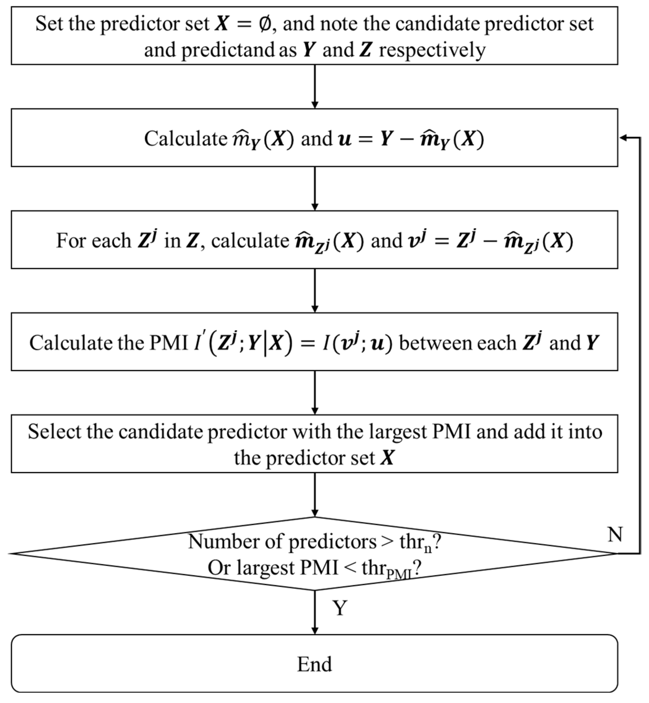
Based on the previous equations, the process of the predictor selection method based on the MI and PMI, named PMIS, is showed in
Figure 1. The
and
are sated thresholds.
2.1.2. Total Mutual Information
The PMIS can be proposed to select suitable predictors from numerous candidate variables, but the PMI cannot reflect the relation between the whole predictor set and the predictand, and the MI cannot reflect the internal relationship among the predictor set. Therefore, the total mutual information (TMI) is developed based on the PMIS method to reflect the relation between the whole predictor set and the predictand. The TMI can be calculated by the following equation:
where
is the number of selected predictors;
is the order of selecting the predictor;
and
are the weight and PMI value of the
ith selected predictor.
The
can be determined by calculating the information gain after introducing the specific predictor. Considering the residual shown in equation (4) can represent the uncertainty in the predictand to some degree, the difference between standard deviation of the residual is used to represent the information gain. Then the
can be calculated as follows:
where
represent the predictor set after introducing the
ith predictor; std denote the standard deviation.
2.2. Case Study and Data Preparing
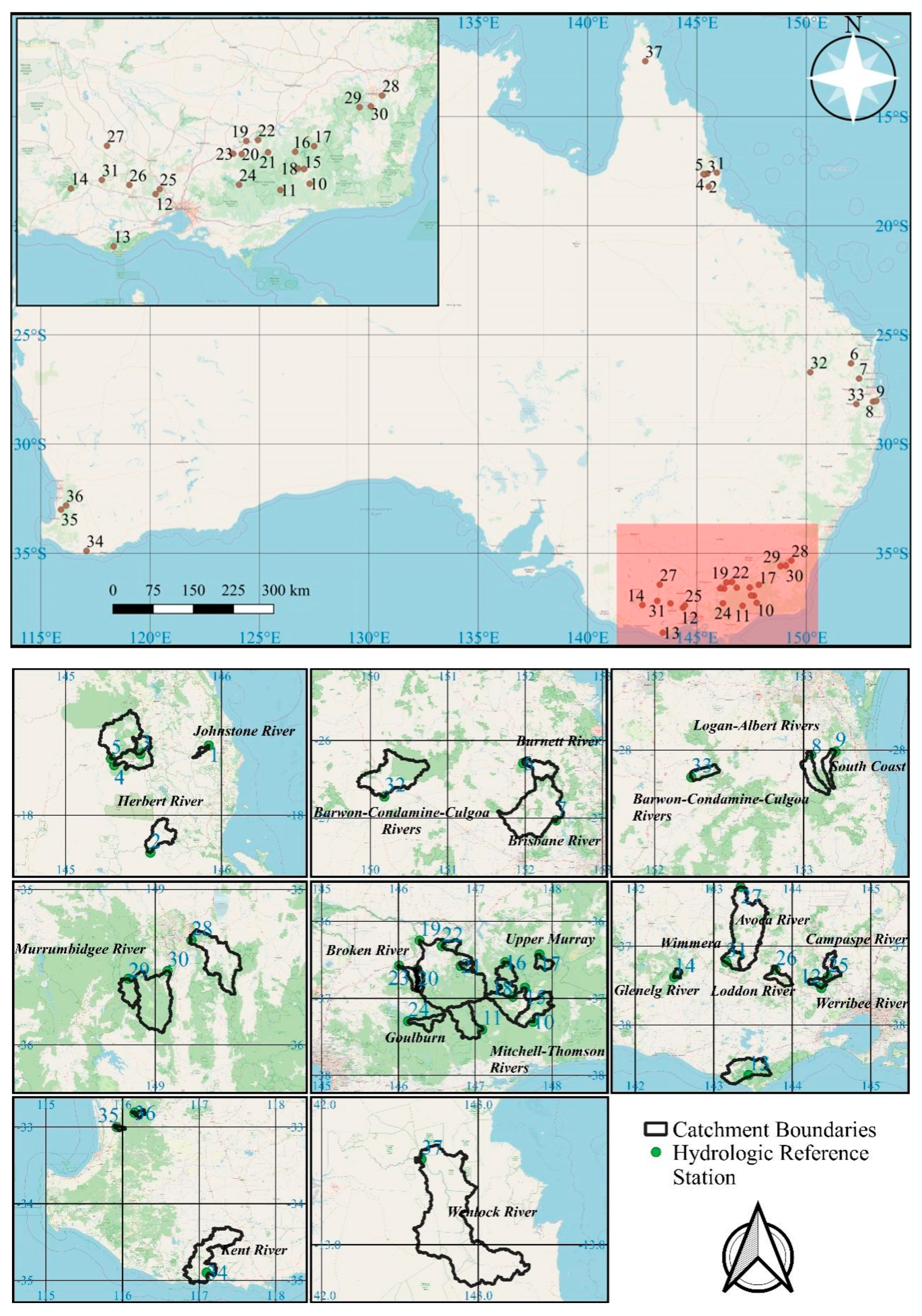
In order to analyze the relationship between TMI and the predictive performance of MLTRP, the predictions are generated in 37 hydrologic reference stations in Australia. The 37 hydrologic reference stations are selected from 221 stations with the best data quality and available data length. All stations are located in catchments with minimal anthropogenic interruptions. The 37 stations and corresponding catchments are shown in Figure 2.
Figure 2.
Locations of the catchments and hydrologic reference stations.
Figure 2.
Locations of the catchments and hydrologic reference stations.
The monthly runoff data of the 37 selected stations can be obtained from the website of Bureau of Meteorology, Australia (
http://www.bom.gov.au/water/hrs/). The available runoff records all end in December 2014 and the start months of different stations are between January 1951 and July 1982. In order to process the skewness in runoff data, the runoff data are preprocessed by a widely used log-sinh data transformation method [
51,
55,
56]. And it should be noted that the following results are demonstrated and discussed based on the transformed data in order to compare the model’s predictive performance among different basins.
The other data used in this study include the rainfall and 130 climate factors. The grid rainfall data with 0.05° resolution are obtained through Australian Water Availability Project (
http://www.auscover.org.au/purl/australian-gridded-climate-data) and processed to monthly area rainfall. The 130 climate factors data are obtained from the website of National Climate Center, China Meteorological Administration (
http://cmdp.ncc-cma.net/en/). The climate data are normalized by:
where
is the original data,
is the transformed data,
year and
month represent time,
is mean value and
is standard deviation.
2.3. Forecasting Models and Model Development Process
2.3.1. Forecasting Models
Five AI models are used to generate mid-long term runoff predictions in this study. The five models are multilayer perceptron (MLP) model, block-based MLP (MB) model, Bayesian SVR (BSVR) model, coupled model of BSVR and ARD kernel (BSVRARD), and long short-term memory (LSTM) model. Because these five models have been widely used in many fields, the details of these five models are not introduced in this study and can be found in other previous studies [
24,
49,
57,
58,
59,
60]. The features of these five models are briefly summarized in
Table 1. In general, the MLP, BSVR and BSVRARD more focus on the point information and the inputs of these models are simple point structure [
49]. The MB and LSTM more focus on the time series information and the inputs of these two models are time series structure [
49].
2.3.2. Model Development Process
The commonly used model development process introduced in [
49,
50] is proposed and modified in this study. Firstly, the PMIS method is used to select predictors and organized to meet the input format requirement of the five models. Meanwhile, the TMI and MI are calculated along with the PMIS process. Secondly, the leave-one-year-out cross validation is applied in this study to generate predictions in whole dataset of each station. Thirdly, the five models are constructed and validated.
The validation metrics include: 1) root mean square error (RMSE) and 2) relative root mean square error (RRMSE). The two metrics can be calculated according to the following equations.
where
and
are the predicted and observed value respectively,
is the number of validation data,
is the standard error.
Because the can represent the predictive performance of a model using the average value as predictions (named average model), the RRMSE, which is the ratio of the RMSE of a specific model to , can represent the forecasting model’s applicability to some degree. A RRMSE value larger than 1 means that the model’s predictive performance is worse than the average model and cannot generate valuable predictions.
2.4. Experiment Setup
In order to examine the ability of TMI in evaluating the applicability of MLTRP, two experiments are implemented in this study and summarized in
Table 2. The main difference of the two experiments is the candidate predictor set. In experiment 1 (E1), the candidate predictions include 130 climate factors and transformed runoff in the previous 12 months. In experiment 2 (E2), the candidate predictors include those in the E1 and area rainfall in the previous 12 months and future
FLT (forecast lead time) months. Based on the candidate predictors, five AI models are used to predict runoff of the 37 stations in the future 1-6 months (37*6=222 forecasting scenarios), and the RMSE and RRMSE are used to evaluate the predictive performance. Meanwhile, the MI and TMI are calculated. Finally, the relationships of RMSE-TMI, RRMSE-TMI and RRMSE-MI are analyzed. In addition, the TMI and predictive performance are further compared between the two experiments.
3. Results
The results of the five forecasting models without and with rainfall in candidate predictors (i.e., E1 and E2) are presented in terms of the RMSE and RRMSE in section 3.1 and section 3.2 respectively.
3.1. The Predictive Performance of Five Models without Rainfall in Predictors
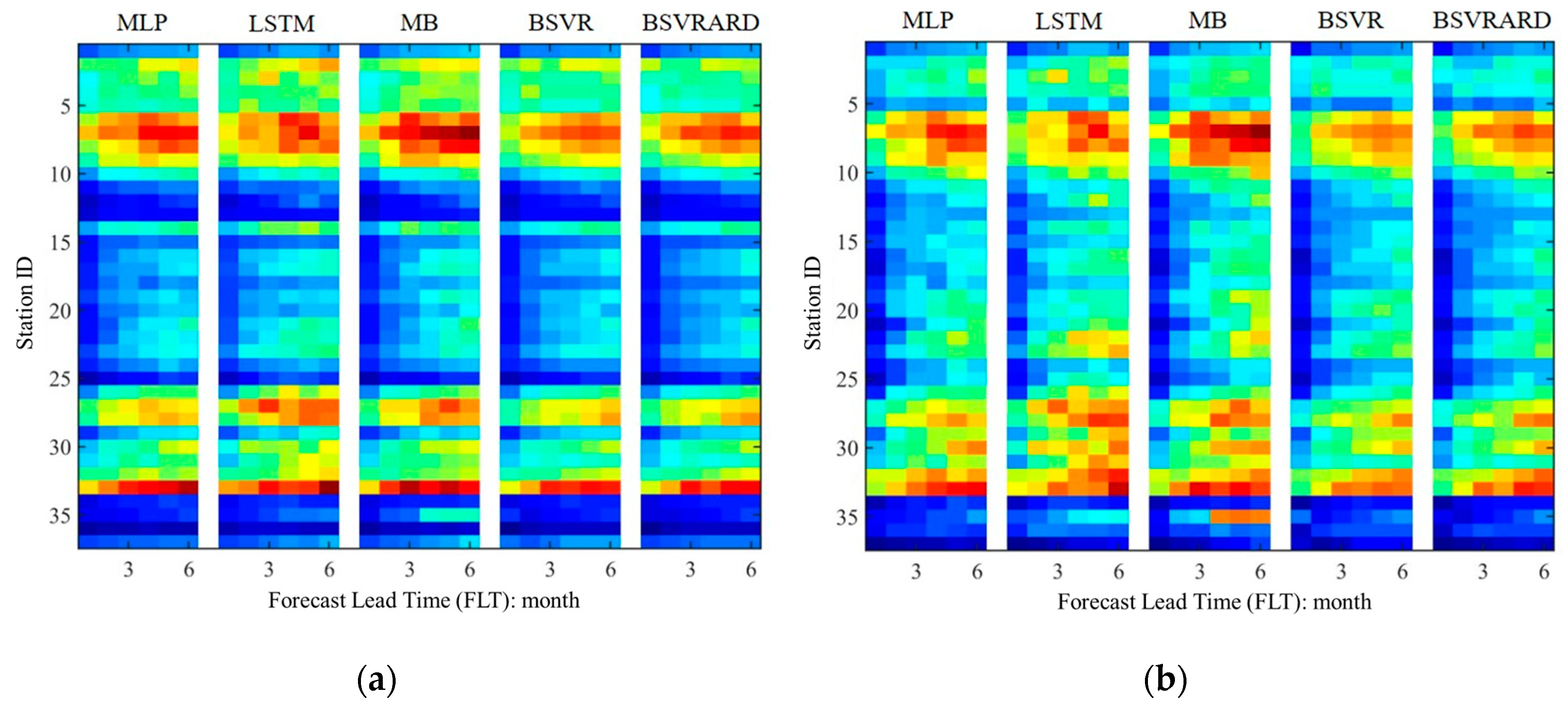
The cross-validated predictive performance of the five AI models (i.e., MLP, LSTM, MB, BSVR and BSVRARD) are examined using the root mean square error (RMSE) and relative root mean square error (RRMSE) obtained over the validation data, as shown in Figure 2. In the figure, the x-axis and y-axis represent the FLT and station ID, and the color represents the RMSE and RRMSE values. The difference of predictive performance results from the difference among basins, FLTs and models. It can be seen from the Figure 2 that the difference of predictive performance caused by the difference of basins is most significant. In addition, the basins with smaller RMSE values and the basins with smaller RRMSE values are different due to the characteristics of the transformed runoff time series. In terms of the influence of the FLT, it can be seen that the all model will obtain best predictive performance, which will become worse along with the increase of FLT. In general, it is obvious that the difference of predictive performance caused by the difference of forecasting scenarios (different basins and different FLTs) is more significant than that caused by the models.
Figure 2.
The RMSE and RRMSE values over the validation data for predicting in the future 1-6 months in the 37 stations without observed rainfall as predictors (E1). (a) RMSE; (b) RRMSE.
Figure 2.
The RMSE and RRMSE values over the validation data for predicting in the future 1-6 months in the 37 stations without observed rainfall as predictors (E1). (a) RMSE; (b) RRMSE.
3.2. The Predictive Performance of Five Models with Rainfall in Predictors
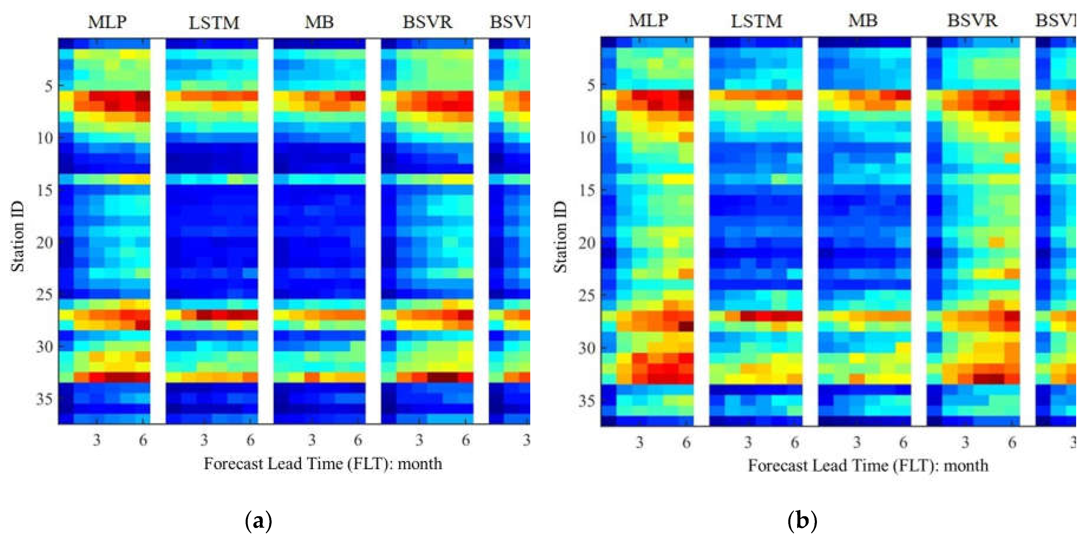
The cross-validated predictive performance of the five AI models are examined using the RMSE and RRMSE obtained over the validation data with rainfall as predictors, as shown in
Figure 3. It can be seen that RMSE values of the 222 forecasting scenarios (37 stations * 6 FLTs) is within 0.4-2.3 and significantly decrease compared with those obtained in experiment 1 (E1, without rainfall as predictors) shown in
Figure 2. And the RRMSE values decrease from 0.35-1.25 (
Figure 2) to 0.2-0.85 (
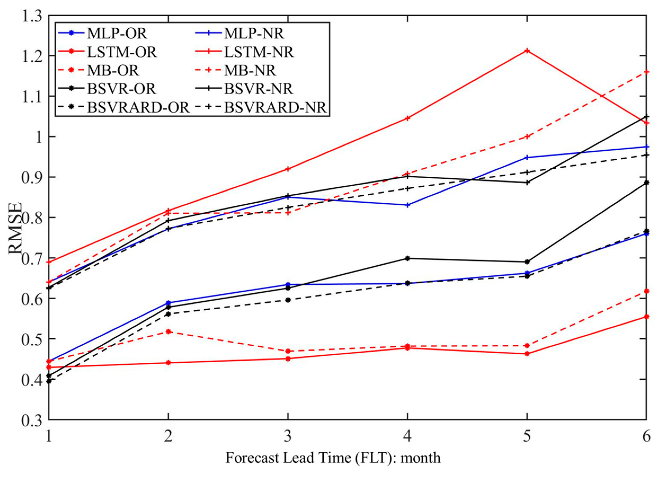
Figure 3). In addition, the difference of predictive performance among different basins is still significant. In terms of the influence of FLTs on predictive performance, different models show different features, which can be seen from
Figure 4. In E2, where the observed rainfall is included in predictors, the predictive performance becomes worse significantly for the MLP, BSVR and BSVRARD models (i.e., point models) along with the increase of FLTs. But the predictive performance of the time series models (i.e., MB and LSTM) are steadier among different FLTs. In E1, the predictive performance of all models shows similar trend with the increase of FLT. Though the LSTM and MB models perform worse in E1, the two models have better performance after the incorporation of rainfall (E2). In addition, the advantages of the time series models (MB and LSTM) compared with the point models (MLP, BSVR and BSVRARD) are more obvious along with the increase of FLT.
4. Discussion
The results are discussed in this section. First, the five models are compared in terms of the predictive performance in section 4.1. Second, the relationship between the total mutual information (TMI) and the predictive performance of five models is analyzed in section 4.2. Finally, the influence of the incorporation of rainfall on the predictive performance is discussed in section 4.3.
4.1. The Comparison of Different Models
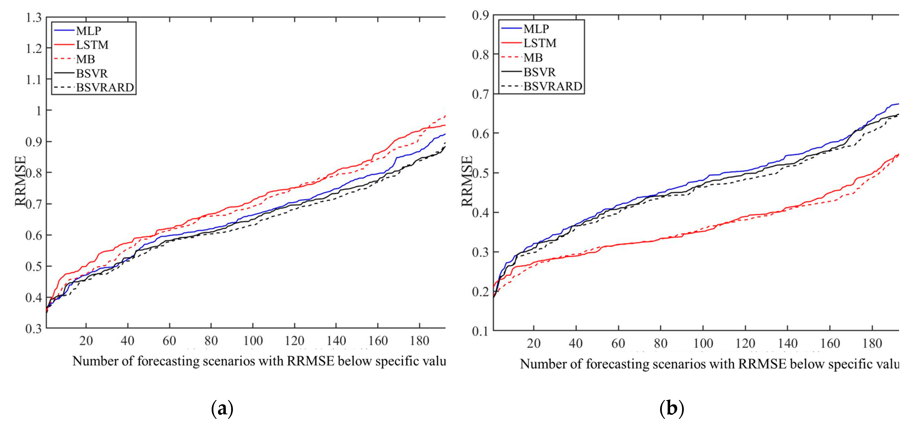
The predictive performance of the five models (i.e., MLP, LSTM, MB, BSVR and BSVRARD) in terms of the RRMSE in 222 forecasting scenarios (37 stations * 6 FLTs) without rainfall in the predictors (E1) is illustrated in
Figure 5(a), and that in E2 is illustrated in
Figure 5(b). In
Figure 5, the y-axis shows the values of the RRMSE and the x-axis shows the number of forecasting scenarios with RRMSE below specific values. It can be seen from
Figure 5(a) that in the three neural network models (MLP, LSTM and MB), the MLP model perform best and the LSTM model perform worst. Though the LSTM models have better performance than the simple machine learning models in many fields, such as flood prediction and rainfall-runoff modelling, some studies also demonstrate that the effect of LSTM depends on the available data [
23,
49,
61]. In MLTRP, the data are all monthly runoff and the limited data may be not enough to support the application of LSTM model. Furthermore, the LSTM are widely used in short term runoff prediction, where the predictand (runoff) has clear physical correlation with the predictors (rainfall and temperature). But in this study, the forecasting models are constructed based on the teleconnection between monthly runoff and climate factors in E1, where the rainfall is not included in predictors. Due to both the limited data and weak connection between predictors and predictand in the MLTRP, the most complex LSTM model performs worst and the complex MB model is worse than the MLP model. But the opposite comparison result can be obtained in E2, as shown in
Figure 5(b). It is obvious that the LSTM and MB models are significantly better than the other three models (i.e., MLP, BSVR and BSVRARD). The main difference between E1 and E2 is that the rainfall is incorporated into the predictors. After the application of rainfall, there is strong physical connection between predictors and predictand. This makes the complex models, which can use the time series information, perform better. In terms of the comparison among the three point models (MLP, BSVR and BSVRARD), the BSVR and BSVRARD models are better than the MLP model, because the uncertainty risks of the model structure and parameters are incorporated in the SVR model and the solution of SVR model is globally optimized [
62].
4.2. The Relationship between Predictive Performance and TMI, MI
4.2.1. RRMSE and MI in E1
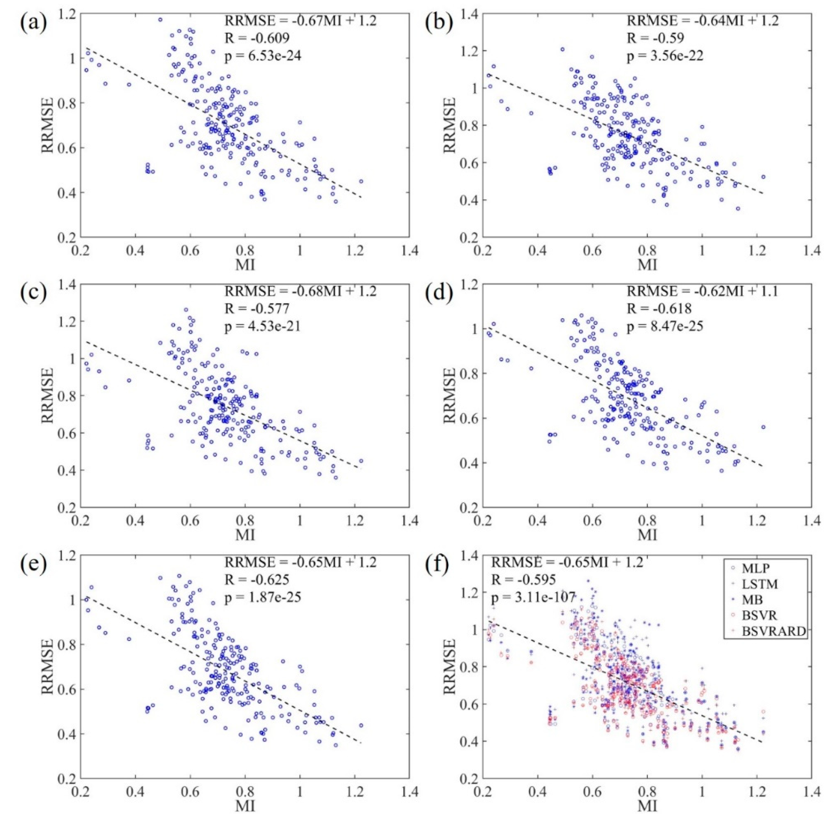
The RRMSE values of 222 forecasting scenarios and the corresponding MIs are shown in
Figure 6, where the linear regression equation and p values are also illustrated. It can be seen that there is a good linear correlation relationship with correlation coefficient around -0.6 and p value less than 4.53×10
-21. This means that there is close connection between the predictive performance and the available information in the predictors, which can be represented by the MI. Even if the RRMSE and MI values are combined in the
Figure 6(f), there is still a good linear correlation relationship. This means that the predictive performance difference caused by the model’s difference is not significant compared with that caused by the difference among MIs. The overall linear regression equation is RRMSE = -0.65*MI + 1.2, which means that the RRMSE is 1.2 showing the model is worse than an average model when the MI is zero. Thought the MI can represent the available information in the predictors to some degree and there is a good correlation between RRMSE and MI, the correlation is not very significant and needs to be further imporved.
4.2.2. RMSE, RRMSE and TMI
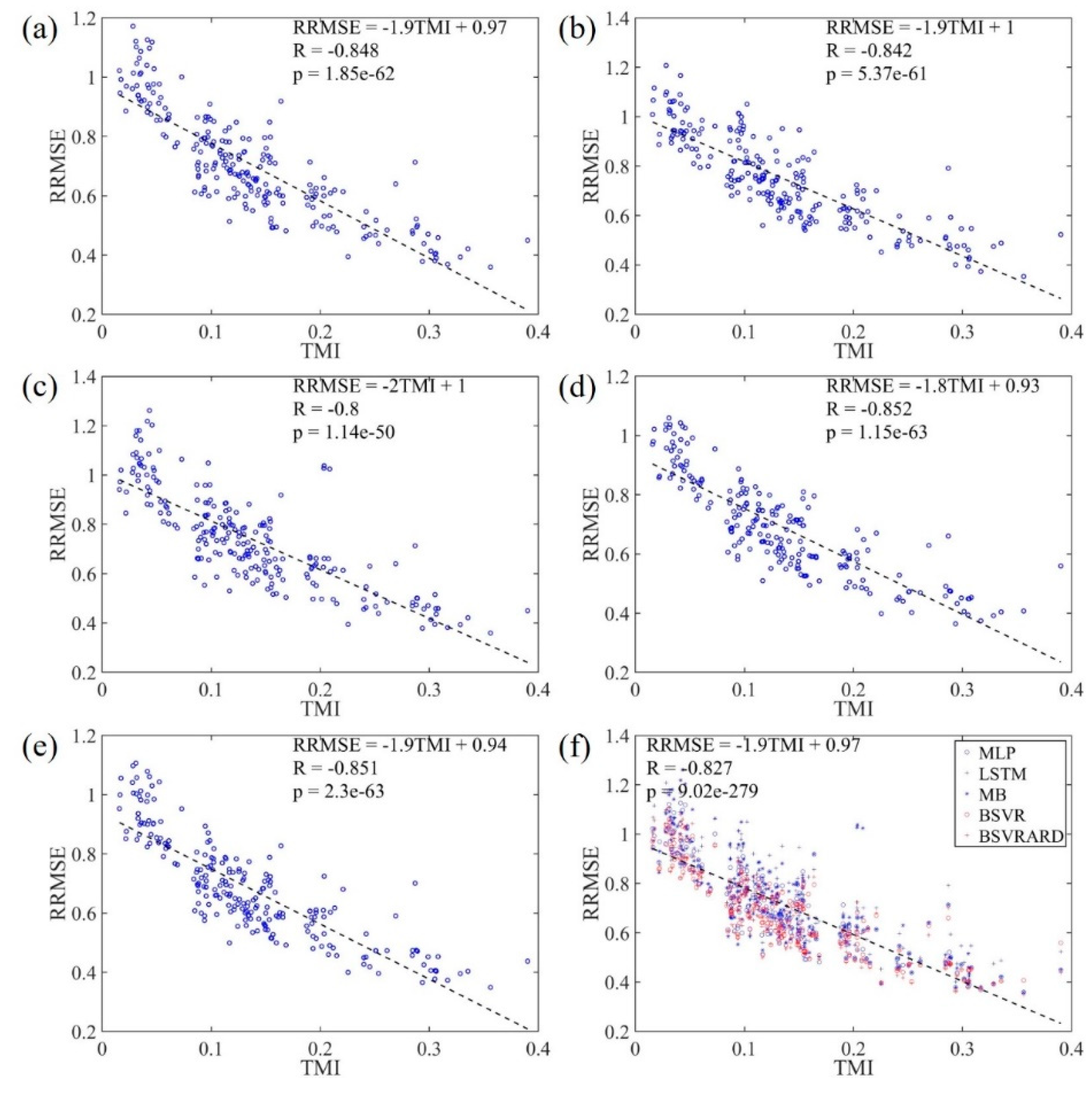
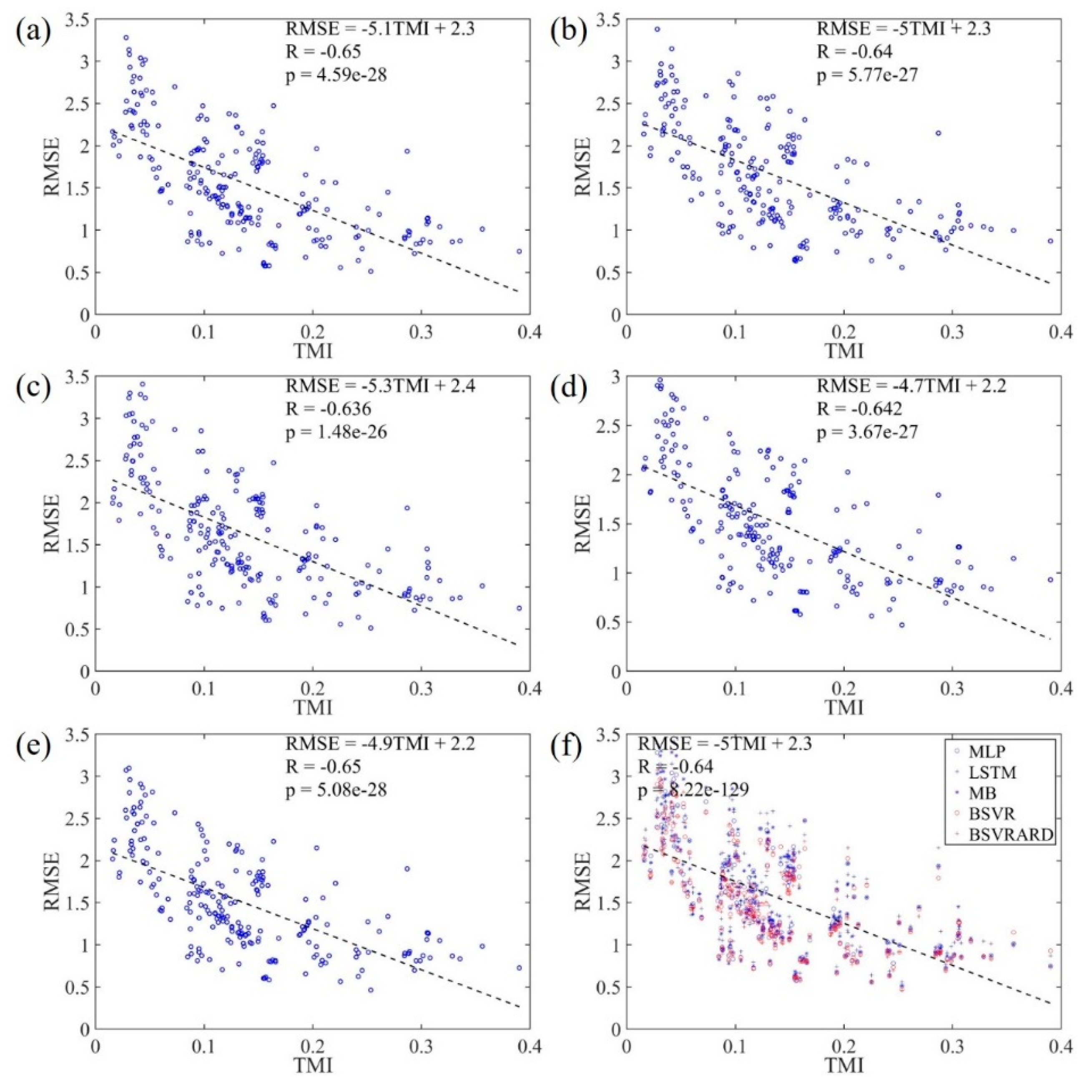
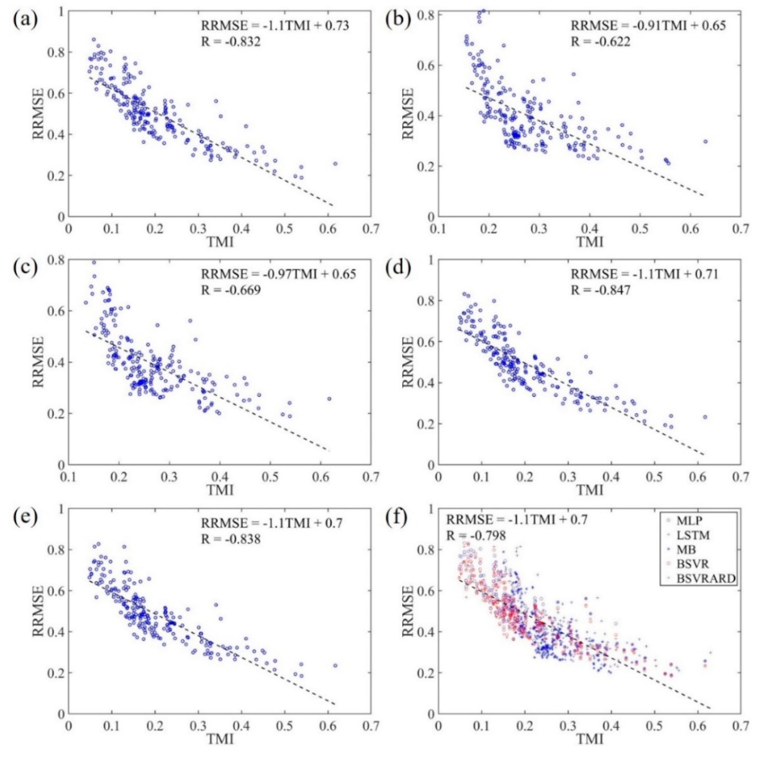
The RRMSE and RMSE values of 222 forecasting scenarios and the corresponding TMIs are shown in
Figure 7 and
Figure 8 respectively. It is clear that the RMSE has negative correlation with the TMI, and the correlation coefficient is around -0.65 with p value less than 1.48×10
-26. However, the RMSE in affected by not only the available information in the predictors (TMI or MI) but also the statistical characteristics of the transformed runoff time series. Therefore, the RRMSE, which is calculated through dividing RMSE by standard deviation of the time series, has a stronger negative correlation with the TMI, which can be seen in
Figure 7. The correlation coefficients are between -0.8 and -0.85 with p values less than 1.14×10
-50. Compared with the correlation coefficients of RRMSE-MI (
Figure 6) and RMSE-TMI (
Figure 8), the correlation coefficients of RRMSE-TMI are closer to -1. This means that the TMI can better represent the available information in the predictors compared with the MI. The main difference between MI and TMI is the way to discriminate the predictors. The MI is used to evaluate the mutual information between all predictors and predictand, but it cannot discriminate the importance of predictors. The TMI is calculated by multiplying the PMIs of predictors with weights which represent the information gain after incorporating the predictor. Therefore, the TMI can discriminate the predictors and better represent the available information.
Because the TMI can represent the available information in the predictors and has strong correlation with the predictive performance, the TMI can be used to evaluate the applicability of MLTRP in a specific forecasting scenario. If the TMI is smaller, it is inappropriate to make mid-long term runoff predictions using data-based models. It can be seen from
Figure 7 that the RRMSE values of almost all models is less than 1 when the TMI is more than 0.1. This means the model can generate valuable forecasting information compared with the average model using average value as predictions. When TMI is less than 0.1, the RRMSE may be more than 1 in some forecasting scenarios. In addition, considering the linear regression equation RRMSE = -1.9TMI + 0.97, the corresponding RRMSE is 0.78 with TMI equal to 0.1, which means the predictive performance is good.
In general, the predictive performance shows strong correlation with the TMI which represents the available information in the predictors, and therefore the TMI can be used to evaluate the applicability of MLTRP. The TMI more than 0.1 may represent the corresponding forecasting scenario is suitable for applying data-based model to generate valuable predictions.
4.2.3. The Linear Regression Equations between RRMSE and MI, TMI
The linear regression equations between RRMSE and MI, TMI are shown in
Figure 7 and
Figure 8 and the slopes and intercepts are summarized in
Table 3. It can be seen that the intercepts are around 1.2 when MI is the independent variable and around 1 when TMI is the independent variable. When the predictor set is empty, the MI and TMI are 0 and the fitted RRMSE values should be 1.2 and 1 respectively. Meanwhile, the forecasting results show be the average values of the time series and the real RRMSE of forecasting model should be 1. From this perspective, the TMI can represent the predictive performance better.
It can also be seen from
Table 3 that the slopes differ among different models. The difference of slopes can partly explain the difference of five models. A less slope value (larger absolute value) means the model is more sensitive to the available information in the predictors. For the MB and LSTM models, the slope is less than the BSVR and BSVRARD model, because these models are more able to use the information in the predictors. For the MLP, the model’s predictive performance is also sensitive to the TMI because the model may fall in local optima and the model performance is not stable.
4.3. The Influence of Rainfall on the Predictive Performance and TMI
In E2, where the rainfall is included in predictors, five models’ predictive performance become better significantly, which may be reflected by the change of TMI. Therefore, the RRMSE and TMI values in E2 are calculated and shown in
Figure 9. It can be seen from the
Figure 9 that the TMI values are between 0.05 and 0.65 and the RRMSE values are between 0.2 and 0.9 after incorporating the rainfall into the predictor set. Compared with the results obtained without rainfall in predictors (
Figure 7), the TMI values increase 0.01-0.31 and the corresponding RRMSE decrease -0.01-0.69. It can also be seen from
Figure 9 that the RRMSE levels off when along with the increase of TMI.
After the incorporation of rainfall, the five models show different features. For the LSTM and MB models, the TMI values are all more than 0.1, and the RRMSE values are less than 0.8. But for the MLP, BSVR and BSVRARD models, there still exists 13.5 forecasting scenarios where the TMI is less than 0.1 and the RRMSE values are around or more than 0.8. The reason for the difference of TMI among the five models is that the time series information is used in the LSTM and MB models.
It can be seen from
Figure 9 that there is still significant negative correlation between the RRMSE and TMI. For the three point models (MLP, BSVR and BSVRARD), the correlation coefficients are around -0.83. But for the LSTM and MB models, the correlation coefficients are -0.62 and -0.67 respectively. The difference of five models in terms of the coefficients is caused by the difference among the model structure. The LSTM and MB models use time series data as model input. But the time series characteristics are not considered in the calculation of PMIS, and therefore the TMI can only partly explain the available information in the input time series data. Nevertheless, the overall correlation coefficient for all five models is -0.80.
5. Conclusions
In this study, the total mutual information (TMI) index is developed based on the predictor selection method named PMIS, which recognize predictors based on the mutual information (MI) and partial MI (PMI). In order to examine the relationship between the TMI and the predictive performance, five AI models (MLP, LSTM, MB, BSVR, BSVRARD) are applied in 37 hydrological stations in Australia to predict monthly runoff in the future 1-6 months, and the RMSE and RRMSE are used to evaluate the predictive performance in 222 forecasting scenarios. The relationship of TMI and RMSE, RRMSE in two different experiments, the difference of which is the application of the rainfall. The main conclusions are as follows:
(1) The developed TMI index can represent the available information in the predictors better than the MI index, and has significant negative correlation with the RRMSE. The correlation coefficients are between -0.8 and -0.85 when the rainfall is not included in predictors. And when the rainfall is included in predictors, the coefficients are between -0.62 and -0.85.
(2) The developed TMI index can be used to evaluate the applicability of MLTRP. Along with the increase of TMI, the available information increases and the model’s predictive performance become better. When TMI is more than 0.1, the available information in the predictors can support the construction of MLTRP models and the model can generate valuable predictions. When TMI is less than 0.1 and near 0, the MLTRP may be not suitable in the forecasting scenarios.
(3) The five AI models have significant different performance in different scenarios. When the rainfall is not included in the predictors, the complex LSTM and MB models using time series as inputs perform worse than the MLP, BSVR and BSVRARD models. After the incorporation of rainfall in predictors, the TMI increases significantly and the complex LSTM and MB models, which can better utilize the contained information in the predictors, perform better than the other three models.
(4) The difference of the five models can be partly explained by the developed TMI index. The slopes of the linear regression equation between the RRMSE of the LSTM and MB models and the TMI are less than those for the BSVR and BSVRARD models. This means the LSTM and MB models are more sensitive to the available information in predictors (i.e., TMI), and therefore the change of model predictive performance for LSTM and MB models are more significant than that of the BSVR and BSVRARD models after the incorporation of rainfall into predictors.
Author Contributions
Conceptualization, S.X. and Z.X.; methodology, S.X. and Z.X.; validation, S.X., Z.X. and Y.W.; investigation, S.X., Y.W. and B.W; data curation, Z.X. and K.S.; writing—original draft preparation, S.X., Z.X., B.W., K.S. and J.W.; supervision, S.X. and Y.W.. All authors have read and agreed to the published version of the manuscript.
Funding
This research was funded by The National Key Research and Development Program of China (No. 2022YFC3202300), the Knowledge Innovation Program of Wuhan – Basic Research (2022020801010240), the Key Project of Chinese Water Resources Ministry (SKS-2022120), the Natural Science Foundation of Hubei Province (2022CFD027), and the National Public Research Institutes for Basic R&D Operating Expenses Special Project (No. CKSF2021486).
Data Availability Statement
The data used in this study are all public and the links to obtain the data are supported in this paper.
Acknowledgments
Various Python open-source frameworks were used in this study. We would like to express our gratitude to all contributors. We would also like to give a special thanks to the anonymous reviewers and editors for their constructive comments.
Conflicts of Interest
The authors declare no conflicts of interest.
References
- Nguyen, Q.H. and V.N. Tran, Temporal Changes in Water and Sediment Discharges: Impacts of Climate Change and Human Activities in the Red River Basin (1958–2021) with Projections up to 2100. Water, 2024. 16(8): p. 1155.
- Jia, L., et al., Sensitivity of Runoff to Climatic Factors and the Attribution of Runoff Variation in the Upper Shule River, North-West China. Water, 2024. 16(9): p. 1272.
- Xu, H., et al., Assessment of climate change impact and difference on the river runoff in four basins in China under 1.5 and 2.0∘ C global warming. Hydrology & Earth System Sciences, 2019. 23(10).
- Zou, L. and T. Zhou, Near future (2016-40) summer precipitation changes over China as projected by a regional climate model (RCM) under the RCP8. 5 emissions scenario: Comparison between RCM downscaling and the driving GCM. Advances in Atmospheric Sciences, 2013. 30(3): p. 806-818.
- Piao, S., et al., The impacts of climate change on water resources and agriculture in China. Nature, 2010. 467(7311): p. 43-51.
- Larraz, B., et al., Socio-Economic Indicators for Water Management in the South-West Europe Territory: Sectorial Water Productivity and Intensity in Employment. Water, 2024. 16(7): p. 959.
- Haj-Amor, Z., et al., Impacts of climate change on irrigation water requirement of date palms under future salinity trend in coastal aquifer of Tunisian oasis. Agricultural Water Management, 2020. 228: p. 105843.
- Shukla, P., et al., Climate Change and Land: an IPCC special report on climate change, desertification, land degradation, sustainable land management, food security, and greenhouse gas fluxes in terrestrial ecosystems. 2019.
- Bărbulescu, A. and L. Zhen, Forecasting the River Water Discharge by Artificial Intelligence Methods. Water, 2024. 16(9): p. 1248.
- Chu, H., J. Wei, and W. Wu, Streamflow prediction using LASSO-FCM-DBN approach based on hydro-meteorological condition classification. Journal of Hydrology, 2020. 580: p. 124253.
- Xie, S., et al., Mid-long term runoff prediction based on a Lasso and SVR hybrid method. Journal of Basic Science and Engineering, 2018. 26(4): p. 709-722.
- Feng, Z.-k., et al., Monthly runoff time series prediction by variational mode decomposition and support vector machine based on quantum-behaved particle swarm optimization. Journal of Hydrology, 2020. 583: p. 124627.
- Sunday, R., et al., Streamflow forecasting for operational water management in the Incomati River Basin, Southern Africa. Physics and Chemistry of the Earth, Parts A/B/C, 2014. 72: p. 1-12.
- Shamir, E., The value and skill of seasonal forecasts for water resources management in the Upper Santa Cruz River basin, southern Arizona. Journal of Arid Environments, 2017. 137: p. 35-45.
- Zhao, H., et al., Investigating the critical influencing factors of snowmelt runoff and development of a mid-long term snowmelt runoff forecasting. Journal of Geographical Sciences, 2023. 33(6): p. 1313-1333.
- Liang, Z., et al., A data-driven SVR model for long-term runoff prediction and uncertainty analysis based on the Bayesian framework. Theoretical and applied climatology, 2018. 133(1-2): p. 137-149.
- He, C., et al., Improving the precision of monthly runoff prediction using the combined non-stationary methods in an oasis irrigation area. Agricultural Water Management, 2023. 279: p. 108161.
- Samsudin, R., P. Saad, and A. Shabri, River flow time series using least squares support vector machines. Hydrology and Earth System Sciences, 2011. 15(6): p. 1835-1852.
- Bennett, J.C., et al., Reliable long-range ensemble streamflow forecasts: Combining calibrated climate forecasts with a conceptual runoff model and a staged error model. Water Resources Research, 2016. 52(10): p. 8238-8259.
- Crochemore, L., M.-H. Ramos, and F. Pappenberger, Bias correcting precipitation forecasts to improve the skill of seasonal streamflow forecasts. Hydrology and Earth System Sciences, 2016. 20(9): p. 3601-3618.
- Jain, A. and A.M. Kumar, Hybrid neural network models for hydrologic time series forecasting. Applied Soft Computing, 2007. 7(2): p. 585-592.
- Firat, M. and M.E. Turan, Monthly river flow forecasting by an adaptive neuro-fuzzy inference system. Water and environment journal, 2010. 24(2): p. 116-125.
- Le, X.-H., et al., Application of long short-term memory (LSTM) neural network for flood forecasting. Water, 2019. 11(7): p. 1387.
- Choi, J., et al., Learning Enhancement Method of Long Short-Term Memory Network and Its Applicability in Hydrological Time Series Prediction. Water, 2022. 14(18): p. 2910.
- Mount, N.J., et al., Data-driven modelling approaches for socio-hydrology: opportunities and challenges within the Panta Rhei Science Plan. Hydrological Sciences Journal, 2016. 61(7): p. 1192-1208.
- Reichstein, M., et al., Deep learning and process understanding for data-driven Earth system science. Nature, 2019. 566(7743): p. 195-204.
- Xie, S., et al., Performance Comparison of Autoregressive Runoff Prediction Methods for Different River Basins. Journal of Basic Science and Engineering, 2018. 26(4): p. 723-736.
- Jónsdóttir, J.F. and C.B. Uvo, Long-term variability in precipitation and streamflow in Iceland and relations to atmospheric circulation. International Journal of Climatology, 2010. 29(10): p. 1369-1380.
- Omondi, P., et al., Linkages between global sea surface temperatures and decadal rainfall variability over Eastern Africa region. International Journal of Climatology, 2013. 33(8): p. 2082–2104.
- Valipour, M., Number of Required Observation Data for Rainfall Forecasting According to the Climate Conditions. American Journal of Scientific Research, 2012. 74: p. 79-86.
- Wang, W.C., et al., A comparison of performance of several artificial intelligence methods for forecasting monthly discharge time series. Journal of Hydrology, 2009. 374(3): p. 294-306.
- Yaseen, Z.M., et al., Artificial intelligence based models for stream-flow forecasting: 2000–2015. Journal of Hydrology, 2015. 530: p. 829-844.
- Yang, T., et al., Developing reservoir monthly inflow forecasts using artificial intelligence and climate phenomenon information. Water Resources Research, 2017. 53(4): p. 2786-2812.
- Kelly, R.A., et al., Selecting among five common modelling approaches for integrated environmental assessment and management. Environmental modelling & software, 2013. 47: p. 159-181.
- Azmi, M., S. Araghinejad, and M. Kholghi, Multi model data fusion for hydrological forecasting using k-nearest neighbour method. Iranian Journal of Science and Technology, 2010. 34(B1): p. 81.
- See, L. and R.J. Abrahart, Multi-model data fusion for hydrological forecasting. Computers & Geosciences, 2001. 27(8): p. 987-994.
- Liu, Y., et al., Mid and long-term hydrological classification forecasting model based on KDE-BDA and its application research. IOP Conference Series: Earth and Environmental Science, 2019. 330: p. 032010.
- Wang, Q., D.E. Robertson, and F.H.S. Chiew, A Bayesian joint probability modeling approach for seasonal forecasting of streamflows at multiple sites. Water Resources Research, 2009. 45(5): p. 641-648.
- Tesfaye, Y.G., M.M. Meerschaert, and P.L. Anderson, Identification of periodic autoregressive moving average models and their application to the modeling of river flows. Water Resources Research, 2006. 42(42): p. 87-94.
- Maity, R., P.P. Bhagwat, and A. Bhatnagar, Potential of support vector regression for prediction of monthly streamflow using endogenous property. Hydrological Processes, 2010. 24(7): p. 917-923.
- Zhang, G. and M.Y. Hu, Neural network forecasting of the British Pound/US Dollar exchange rate. Omega, 1998. 26(4): p. 495-506.
- Coulibaly, P., B. Bobée, and F. Anctil, Improving extreme hydrologic events forecasting using a new criterion for artificial neural network selection. Hydrological Processes, 2010. 15(8): p. 1533-1536.
- Nilsson, P., C.B. Uvo, and R. Berndtsson, Monthly runoff simulation: Comparing and combining conceptual and neural network models. Journal of Hydrology, 2006. 321(1): p. 344-363.
- Kirono, D.G., F.H. Chiew, and D.M. Kent, Identification of best predictors for forecasting seasonal rainfall and runoff in Australia. Hydrological Processes: An International Journal, 2010. 24(10): p. 1237-1247.
- Kashid, S.S., S. Ghosh, and R. Maity, Streamflow prediction using multi-site rainfall obtained from hydroclimatic teleconnection. Journal of Hydrology, 2010. 395(1): p. 23-38.
- Li, H., M. Xie, and S. Jiang, Recognition method for mid-to long-term runoff forecasting factors based on global sensitivity analysis in the Nenjiang River Basin. Hydrological Processes, 2012. 26(18): p. 2827-2837.
- Zhang, D., et al., Modeling and simulating of reservoir operation using the artificial neural network, support vector regression, deep learning algorithm. Journal of hydrology (Amsterdam), 2018. 565: p. 720-736.
- May, R., G. Dandy, and H. Maier, Review of input variable selection methods for artificial neural networks. Artificial neural networks-methodological advances and biomedical applications, 2011. 10: p. 16004.
- Xie, S., et al., Artificial neural network based hybrid modeling approach for flood inundation modeling. Journal of Hydrology, 2021. 592: p. 125605.
- Wu, W., G.C. Dandy, and H.R. Maier, Protocol for developing ANN models and its application to the assessment of the quality of the ANN model development process in drinking water quality modelling. Environmental Modelling & Software, 2014. 54: p. 108-127.
- Zhao, T., A. Schepen, and Q.J. Wang, Ensemble forecasting of sub-seasonal to seasonal streamflow by a Bayesian joint probability modelling approach. Journal of Hydrology, 2016. 541: p. 839-849.
- Hejazi, M.I. and X. Cai, Input variable selection for water resources systems using a modified minimum redundancy maximum relevance (mMRMR) algorithm. Advances in water resources, 2009. 32(4): p. 582-593.
- May, R.J., et al., Application of partial mutual information variable selection to ANN forecasting of water quality in water distribution systems. Environmental Modelling & Software, 2008. 23(10-11): p. 1289-1299.
- May, R.J., et al., Non-linear variable selection for artificial neural networks using partial mutual information. Environmental Modelling & Software, 2008. 23(10-11): p. 1312-1326.
- Wang, Q., et al., A log-sinh transformation for data normalization and variance stabilization. Water Resources Research, 2012. 48(5).
- Wang, Q., et al., A Seasonally Coherent Calibration (SCC) Model for Postprocessing Numerical Weather Predictions. Monthly Weather Review, 2019. 147(10): p. 3633-3647.
- Gestel, T.V., et al. Automatic relevance determination for least squares support vector machine regression. in Neural Networks, 2001. Proceedings. IJCNN’01. International Joint Conference on. 2001. IEEE.
- Gestel, T.V., et al., Financial time series prediction using least squares support vector machines within the evidence framework. IEEE Transactions on neural networks, 2001. 12(4): p. 809-821.
- Gestel, T.V., et al., Bayesian framework for least-squares support vector machine classifiers, Gaussian processes, and kernel Fisher discriminant analysis. Neural computation, 2002. 14(5): p. 1115-1147.
- Hochreiter, S. and J. Schmidhuber, Long short-term memory. Neural computation, 1997. 9(8): p. 1735-1780.
- Kratzert, F., et al., Rainfall–runoff modelling using long short-term memory (LSTM) networks. Hydrology and Earth System Sciences, 2018. 22(11): p. 6005-6022.
- Lin, J., C. Cheng, and K. Chau, Using support vector machines for long-term discharge prediction. Hydrological Sciences Journal, 2006. 51(4): p. 599-612.
|
Disclaimer/Publisher’s Note: The statements, opinions and data contained in all publications are solely those of the individual author(s) and contributor(s) and not of MDPI and/or the editor(s). MDPI and/or the editor(s) disclaim responsibility for any injury to people or property resulting from any ideas, methods, instructions or products referred to in the content. |
© 2024 by the authors. Licensee MDPI, Basel, Switzerland. This article is an open access article distributed under the terms and conditions of the Creative Commons Attribution (CC BY) license (http://creativecommons.org/licenses/by/4.0/).
