Optimal Harvesting Strategies for Timber and Non-timber Forest Products with Nonlinear Harvesting Term

Preprint

Article

Optimal Harvesting Strategies for Timber and Non-timber Forest Products with Nonlinear Harvesting Term

This version is not peer-reviewed.

This version is not peer-reviewed.

Altmetrics

Downloads

Views

Comments

Submitted:

09 May 2024

Posted:

10 May 2024

You are already at the latest version

A peer-reviewed article of this preprint also exists.

Abstract

Forest resources are renewable,rational exploitation and utilization of forest resources are not only conducive to sustainable development of population, but also can obtain higher economic benefits. Based on actual timber harvesting problems,a combined harvesting model of timber and non-timber with nonlinear harvesting term was established.Firstly, using the qualitative theory of ordinary differential equations, the dynamic behavior of the model is studied, and the existence and stability of the equilibrium point of the model are proved .Secondly, the optimal control solution is obtained by using the optimal control theory.Finally, the optimal harvesting strategy of timber and non-timber products is given based on the numerical simulation results, which provides a certain theoretical basis for the sustainable development of forestry ecological economy.

Keywords:

Subject:

Computer Science and Mathematics - Mathematics

0. Introduction

Population dynamics is one of the branches of biomathematics, which focuses on the quantitative, spatial and structural dynamics of populations, and can be used to describe the dynamic relationships between populations and their environment and between populations and other populations, as well as to explain, predict, regulate and control the developmental processes and trends of species [1]. The updating and development of biological population dynamics models have effectively contributed to the human knowledge of biological systems. At present, many scholars have established mathematical models to judge and predict the stable development of populations, such as forestry, agriculture, fisheries, integrated control and management of pests, etc., which have given us practical production life [2,3,4].

The problem of optimal control of ecosystems has been a major concern. The problem of optimal control of ecosystems has been one of the hot issues studied by scholars. The maximum sustainable yield policy obtained by studying the optimal harvesting of biological populations is an important ecological management tool to protect the survival of populations and to maximize economic benefits [5,6].

Forests are important natural resources, which not only provide the necessary economic support for human production and life, but also play a role in regulating the climate, water conservation, air purification and biodiversity conservation. In recent years, the increasing demand of timber market and the intensification of commercial exploitation have led to the over-harvesting of forest resources, and the balance of timber and forest products supply has been greatly damaged. In order to ensure the sustainable development of forest resources, a series of logging policies have been established in various regions, and it is therefore necessary to develop reasonable timber harvesting strategies to obtain higher ecological benefits. However, because of such restrictions, it may not be economically viable to provide sufficient income for local residents and timber harvesters. Non-timber products such as fruits, seeds, leaves, bark, gum, etc., can also generate significant economic and ecological benefits, and can even generate more economic income than timber harvesting or agricultural production. Therefore, the study of the ecological impacts of non-timber forest products utilization is also very important for the sustainable use of forest resources and biodiversity conservation [7]. Most of the previous studies have been devoted to timber harvesting, while non-timber harvesting has been studied less frequently and in a discontinuous manner. For example, in 2011, Isabel B et al. [8] modeled the ecological impacts of harvesting non-timber products using stage structure matrix models based on projection matrices. Although these models can quantify the effects of different life stages on plant population dynamics, they do not explicitly represent harvest intensity, which poses a challenge to quantify the effects of harvest intensity on each stage transition. In addition, matrix models have more parameters than classical logistic growth models and may be difficult to relate to well-established harvesting theories based on logistic growth models. Therefore, this paper investigates the problem of joint harvesting of timber and non-timber products based on the current exploitation status of the relevant background of timber and non-timber products in forests, so as to derive the optimal harvesting strategy that is conducive to the conservation and recovery of populations.

1. Model Building

In 2016, Gaoue et al. [9] developed a joint harvest model for timber and non-timber products based on a logistic timber growth equation with proportional harvest, which is the first continuous theoretical model for non-timber harvest

\{\begin{cases} \frac{d x}{d t} = r x (1 - \frac{x}{K}) - h_{L} x \\ τ \frac{d r}{d t} = r_{e} - r - α h_{N} - β h_{L}, \end{cases}

(1)

The model includes harvesting of timber and non-timber products, and additional synergistic effects of harvesting on the growth rate of plant populations. It is also shown that the sustainability of timber and non-timber harvests depends on the effect of harvesting on species growth rates for each type of population, and that there are two states in this differential equation,

x

denotes the population density,

r

represents the endogenous growth rate of the plant, and

r_{e}

is the maximum growth rate in the absence of harvest. The population

x

has logistic growth and

K

is the environmental holding capacity.

h_{L}

is the timber harvest intensity,

h_{N}

is the non-timber harvest intensity,

τ

is the average population longevity,

α

is the population decay rate due to non-timber harvest, and

β

is the population decay rate due to timber harvest.

The harvest term of the first differential equation in this model uses proportional harvesting, but in practical ecological problems, the human catch does not increase infinitely with the increase of capture effort and biological resources, therefore, more and more scholars have started to study predation systems with nonlinear harvest rates [10,11,12].Agnew [13] considered the competition between fishing vessels as an example of fishery harvesting and The nonlinear harvest term was improved by taking into account the competition among fishing vessels and the processing time of the capture fishery, and for a specific model that conforms to the logistic growth law, a nonlinear catch function term of the following form was given after a simplified analysis.

H (x, E) = \frac{x E}{1 + a_{1} E + a_{2} x},

where

E

is the harvesting effort of timber product,

a_{1}

is used to measure the competition between vessels, and

a_{2}

represents the proportionality constant of the handling time.

The harvesting and processing of timber products is more complicated and requires more processing time, while generally timber needs to establish permits and has fixed contractors, so there is not much competition. Therefore, in this paper, we only consider the timber handling time without considering the competition among harvesters, and simplify the nonlinear harvesting term as follows

H (x, E) = \frac{E_{1} x}{1 + a x},

where,

x

denotes the population density,

E_{1}

is the harvesting effort of timber products, and

a

is the handling time of timber products. Therefore,we introduced the nonlinear harvesting function into the model established by Gaoue et al. and established a harvesting model for timber and non-timber products with nonlinear harvesting function

\{\begin{cases} \frac{d x}{d t} = r x (1 - \frac{x}{K}) - \frac{E_{1} x}{1 + a x}, \\ τ \frac{d r}{d t} = r_{e} - r - α E_{2} - β \frac{E_{1}}{1 + a x} . \end{cases}

(2)

2. Qualitative Analysis

2.1. Existence of Equilibrium Point

Theorem 1.

Equation (2) has a trivial equilibrium point

x_{0} = 0

, and when the condition

r_{e} > α E_{2} + (1 + β) E_{1}

is satisfied, the equation has a unique positive equilibrium point

x^{*}

Proof of Theorem 1.

Considering the harvest of timber and non-timber, the dynamics of the long-term range is in quasi-steady state, therefore

r = r_{e} - α E_{2} - β \frac{E_{1}}{1 + a x},

We use this to reduce equation (2) into the following single equation:

\frac{d x}{d t} = (r_{e} - α E_{2} - β \frac{E_{1}}{1 + a x}) x (1 - \frac{x}{K}) - \frac{E_{1} x}{1 + a x} .

(3)

By discussing equation (3), we have:

(1) The equation always has a trivial equilibrium point.

(2) Otherwise, there is

(r_{e} - α E_{2} - β \frac{E_{1}}{1 + a x}) (1 - \frac{x}{K}) - \frac{E_{1}}{1 + a x} = 0,

it can be obtained

- a (r_{e} - α E_{2}) x^{2} + ((K a - 1) (r_{e} - α E_{2}) + β E_{1}) x + K (r_{e} - α E_{2} - (1 + β) E_{1}) = 0

When the condition

r_{e} > α E_{2} + (1 + β) E_{1}

is satisfied, according to Veda’s theorem

\frac{k (r_{e} - α E_{2} - (1 + β) E_{1}}{- a (r_{e} - α E_{2})} < 0

, there exists a unique positive equilibrium point for the equation.

2.2. Stability of Equilibrium Point

Theorem 2.

Equation (2) has a locally asymptotically stable equilibrium point

x_{0}

r_{e} < α E_{2} + (1 + β) E_{1}

; equation (2) has a unique locally asymptotically stable positive equilibrium point

x^{*}

r_{e} > α E_{2} + (1 + β) E_{1}

is satisfied.

Proof of Theorem 2.

(1) The Jacobian matrix at equilibrium

x_{0}

is given by

J (x) = [r_{e} - α E_{2} - (1 + β) E_{1}],

it can be obtained that the eigenvalues

λ = r_{e} - α E_{2} - (1 + β) E_{1},

thus, where

r_{e} < α E_{2} + (1 + β) E_{1}

, the equilibrium is locally asymptotically stable.

The Jacobian matrix

x^{*}

at the equilibrium is given by

J (x^{*}) = [\frac{x^{*}}{K} (\frac{K a E_{1} (1 + β) + β E_{1}}{{(1 + a x)}^{2}} + α E_{2} - r_{e})],

the eigenvalues is

λ = \frac{x^{*}}{K} (\frac{K a E_{1} (1 + β) + β E_{1}}{{(1 + a x)}^{2}} + α E_{2} - r_{e}),

where

\frac{x^{*}}{K} > 0

,we can get

r_{e} > \frac{K a E_{1} (1 + β) + β E_{1}}{{(1 + a x^{*})}^{2}} + α E_{2},

the condition can be strengthened by taking the maximum value at

x = 0

r_{e} > K a E_{1} (1 + β) + β E_{1} + α E_{2} .

When discussing the existence of the solution, there exists a unique positive equilibrium point

x^{*}

of the equation if

r_{e} > α E_{2} + (1 + β) E_{1}

. At this time, if the positive equilibrium is stable, the condition

r_{e} > K a E_{1} (1 + β) + β E_{1} + α E_{2}

will also be satisfied, and the above analysis holds.

In summary, when condition

r_{e} < α E_{2} + (1 + β) E_{1}

is satisfied, equation (2) has a locally asymptotically stable trivial equilibrium point

x_{0}

. Harvesting timber and non-timber in this case leads to a large decay rate of the plant population, which will eventually lead to extinction if the plant population keeps growing at such a growth rate; when condition

r_{e} > α E_{2} + (1 + β) E_{1}

is satisfied, the equation has a unique positive equilibrium point

x^{*}

, and

x^{*}

is locally asymptotically stable. The plant growth rate is sustainable when combined timber and non-timber harvesting is carried out in this case.

3. Optimal Harvesting Strategy

In this section we consider the issue of harvesting of timber and non-timber products. The economic revenue benefits are maximized while minimizing the harvesting costs of timber and non-timber products, while ensuring the sustainability of system populations. Economic benefits are considered in the objective generalization to establish the optimal control problem.

\begin{array}{l} \max_{E_{1}, E_{2} \in U} J (E_{1}, E_{2}) = A_{T} x (t) + \int_{0}^{T} e^{- δ t} (A x (t) + B_{1} \frac{E_{1} (t)}{1 + a x (t)} x (t) + B_{2} E_{2} (t) x (t) - C_{1} {(\frac{E_{1} (t)}{1 + a x (t)})}^{2} - C_{2} E_{2}^{2} (t)) d t, \\ s . t . \{\begin{cases} \frac{d x (t)}{d t} = r (t) x (t) (1 - \frac{x (t)}{K}) - \frac{E_{1} (t)}{1 + a x (t)} x (t), \\ τ \frac{d r (t)}{d t} = r_{e} - r (t) - α \frac{E_{1} (t)}{1 + a x (t)} - β E_{2} (t), \\ 0 \leq E_{1} (t) \leq 0.7, 0 \leq E_{2} (t) \leq 1, \end{cases} \end{array}

(4)

where,

J

is the objective function of the optimal control problem,and it is desired to find an optimal control pair

(E_{1}^{*}, E_{2}^{*})

such that the objective function is maximized. In addition,the coefficient

B_{1}, B_{2}

denotes the price of the two types of harvesting,

B_{1} \frac{E_{1} (t) x (t)}{1 + a x (t)} + B_{2} E_{2} (t) x (t)

is the corresponding income;

e^{- δ t}

denotes the discount term;

C_{1} {(\frac{E_{1} (t)}{1 + a x (t)})}^{2} + C_{2} E_{2}^{2} (t)

is the cost term, in reference [8] Gaoue et al. used the cost term of harvesting is nonlinear and used the quadratic form of control.In order to facilitate the comparison of the difference between the harvesting strategies corresponding to nonlinear harvesting and proportional harvesting,the quadratic form of control is also used for the cost term in this paper.

The weighting factor

A

balances the importance of stock conservation, and

A_{T} x (t)

indicates the conservation value of the stock at the end of the harvest. The total economic return is

\max_{E_{1}, E_{2} \in U} P (E_{1}, E_{2}) = \int_{0}^{T} e^{- δ t} (B_{1} \frac{E_{1} (t)}{1 + a x (t)} x (t) + B_{2} E_{2} (t) x (t) - C_{1} {(\frac{E_{1} (t)}{1 + a x (t)})}^{2} - C_{2} E_{2}^{2} (t)) d t,

The control set of the Lebesque measurable function boundary of the equation is

u = \{(E_{1}, E_{2}) \in {(L^{\infty} (0, T))}^{2} : 0 \leq E_{1} \leq M_{1}, 0 \leq E_{2} \leq M_{2}, 0 \leq t \leq T\},

where,

M_{1}, M_{2}

is an upper bound on the control, for which the control set and the target generalization have appropriate tightness and convexity assumptions to guarantee the existence of optimal control pairs and corresponding states. The Hamiltonian function constructed here is

\begin{array}{l} H = \int_{0}^{T} e^{- δ t} (A x (t) + B_{1} (t) \frac{E_{1} (t) x (t)}{1 + a x (t)} + B_{2} E_{2} (t) x (t) - C_{1} {(\frac{E_{1} (t)}{1 + a x (t)})}^{2} - C_{2} E_{2}^{2} (t)) \\ + λ_{x} (r (t) x (t) (1 - \frac{x}{K}) - \frac{E_{1} (t)}{1 + a x (t)}) + \frac{λ_{r}}{τ} (r_{e} - r (t) - (α E_{2} (t) + β \frac{E_{1} (t)}{1 + a x (t)}) d t . \end{array}

The concomitant function is derived from Pontryagin’s principle of maximum value as

\begin{array}{l} {λ^{'}}_{x} = - \frac{\partial H}{\partial x} = - e^{- δ t} (A + \frac{B_{1} E_{1} (t)}{{(1 + a x (t))}^{2}} + B_{2} E_{2} (t) + \frac{2 a C_{1} E_{1} (t)}{{(1 + a x (t))}^{3}}) \\ - λ_{x} (r (t) - \frac{2 x (t) r (t)}{K} - \frac{E_{1}}{{(1 + a x (t))}^{2}}) + \frac{λ_{r} β E_{1} (t) a}{τ {(1 + a x (t))}^{2}}, \\ {λ^{'}}_{r} = - \frac{\partial H}{\partial r} = - λ_{x} x (t) (1 - \frac{x (t)}{K}) + \frac{λ_{r}}{τ} . \end{array}

The transversality conditions are

λ_{x} (T) = A_{T}, λ_{r} (T) = 0 .

Also from

\frac{\partial H_{2}}{\partial E_{1}} = 0, \frac{\partial H_{2}}{\partial E_{2}} = 0

,it can be derived that

\{\begin{cases} e^{- δ t} (\frac{B_{1} x (t)}{1 + a x (t)} - \frac{2 C_{1} E_{1} (t)}{1 + a x (t)}) - \frac{λ_{x} x (t)}{1 + a x (t)} + \frac{λ_{r} β}{τ (1 + a x (t))} = 0, \\ e^{- δ t} (B_{2} x (t) - 2 C_{2} E_{2} (t) - \frac{λ_{r} α}{τ} = 0 . \end{cases}

we have

\{\begin{cases} E_{1}^{*} = \frac{B_{1} x (t) (1 + a x (t) - e^{δ t} (1 + a x (t) (λ_{x} x (t) - λ_{r} β)}{2 C_{1}}, \\ E_{2}^{*} = \frac{B_{2} x (t) - α \frac{λ_{r}}{τ} e^{δ t}}{2 C_{2}} . \end{cases}

(5)

For the timber harvesting problem with a nonlinear harvesting term, the objective function can be maximized when the optimal control pair

(E_{1}^{*}, E_{2}^{*})

takes the value of

J

, so that the economic and ecological benefits are optimized.

4. Numerical Simulation

In this section, the optimal harvesting strategy is simulated numerically, and the numerical results of the optimal harvesting strategy with a nonlinear harvesting term are compared with proportional harvesting, and parameter sensitivity analysis is performed. The values of the parameters are shown in Table 1.

5.1. The Effect of Proportional Harvesting and Nonlinear Harvesting on the Optimal Harvesting Strategy

1. Some parameters of proportional harvesting and nonlinear harvesting are taken as

T = 5, τ = 5, r_{e} = 0.25, a = 0.1, A = 0.1, A_{T} = 0.1, δ = 0.05

,see Table 1 for other parameters.

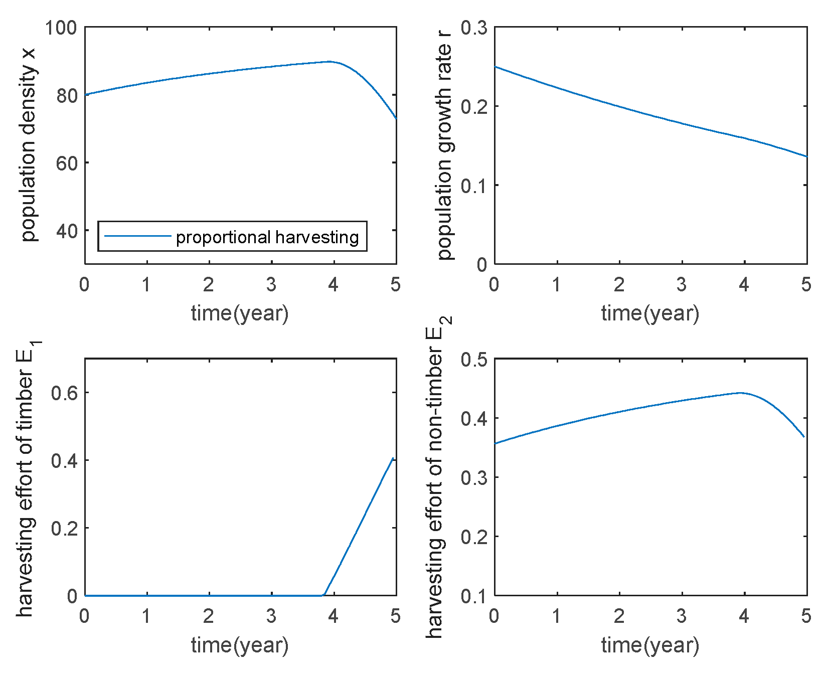
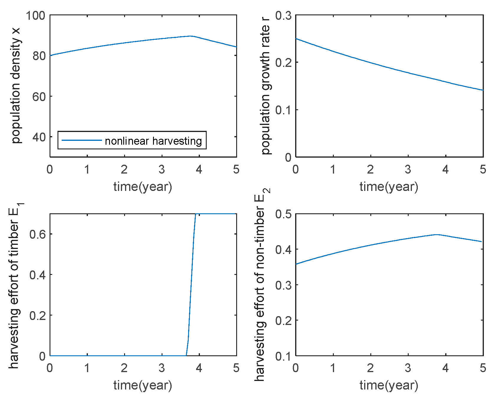
Figure 1 shows the harvesting strategy with proportional harvesting, it can be seen that the timber harvesting starts around the fourth year after the non-timber harvesting starts, and at the end of harvesting, the timber population decreases by about 10%, and the objective function of the optimal control problem has the maximum value of A. Figure 2 shows the non-linear harvesting strategy, it can be seen that when the non-linear harvesting is used, the timber harvesting starts around year 3.7, and at the end of harvesting, the population size is The maximum value of the objective function of the optimal control problem is B. Compared with proportional harvesting, the economic benefit is reduced by 14.87%, but the economic benefit plus ecological benefit is only reduced by 0.8%, which indicates that the nonlinear harvesting method has a great improvement on ecological benefit and is more beneficial to the recovery of the population.

5.2. Sensitivity Analysis of Parameters

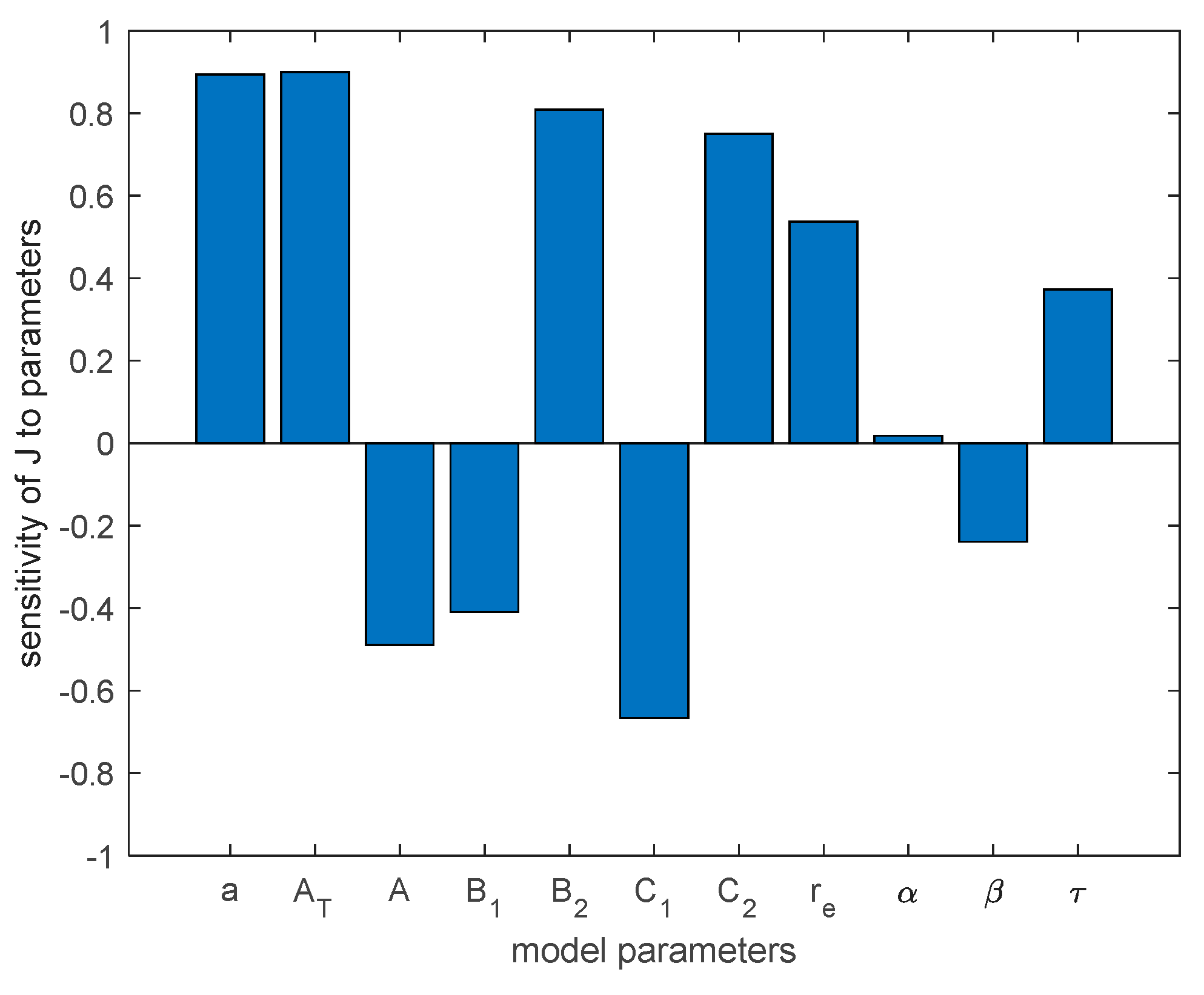
In this section, the sensitivity of the objective function with respect to each parameter is calculated using the partial rank correlation coefficient (PRCC) method for the optimal control problem.

Figure 3 shows the parameter sensitivity analysis of the pair，it can be seen that the importance of population conservation at the end of harvest

A_{T}

has a greater impact on the objective function; at the same time, timber treatment time also has an impact on the objective function, indicating that it is necessary for us to consider timber treatment time; the price and cost of non-timber

B_{2}, C_{2}

also have a greater impact on the sensitivity of

J

, so a combined harvest of timber and non-timber can yield better benefits.

5.3. Effect of Different Parameters on the Optimal Harvesting Strategy

This section focuses on the influence of parameters on the optimal harvesting strategy. The price of timber

B_{1}

, the cost of timber harvesting

C_{1}

, the price of non-timber

B_{2}

, and the cost of non-timber harvesting

C_{2}

are influenced by the market and are not specifically analyzed here.

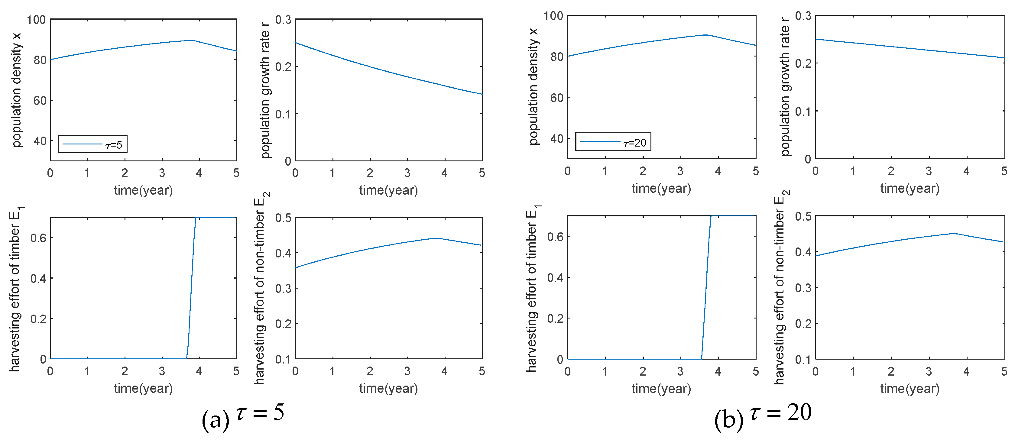
1.The effect of timber processing time on the optimal control strategy, some parameters are taken as

T = 5, τ = 5, r_{e} = 0.25, A = 0.1, A_{T} = 0.1

,see Table 1 for other parameters.

The objective functions of the optimal harvesting strategies for different timber treatment times are

J_{\max} = 60.2475, p_{\max} = 16.8275

J_{\max} = 60.6665, p_{\max} = 19.7374 .

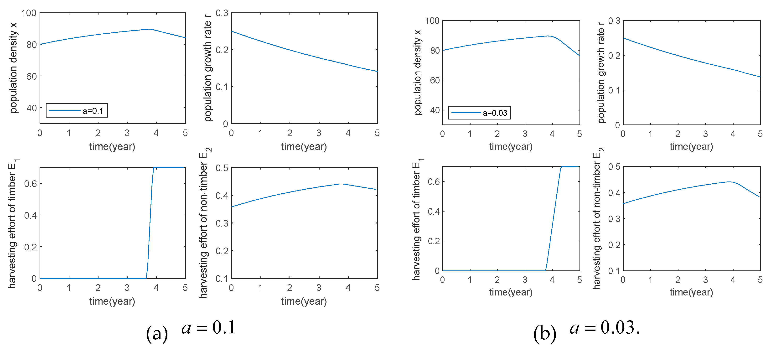
It can be seen from Figure 4 that the timber treatment time has a certain influence on the timber harvesting strategy.The lower the treatment time, the lower the population size at the end of harvest, and the higher the economic benefits, but the lower the ecological benefits.

2.The effect of plant growth rate on the optimal control strategy, some parameters are taken as

T = 5, τ = 20, a = 0.1, A = 0.1, A_{T} = 0.1

,see Table 1 for other parameters.

The objective functions of slow growth and fast growth are

J_{\max} = 54.9543, p_{\max} = 14.8346

;

J_{\max} = 60.918 p_{\max} = 17.1486 .

It can be seen from Figure 5 that species with fast growth rate can obtain higher economic and ecological benefits. Also fast growing species can start harvesting timber earlier and the population size is not reduced at the end of harvest, which can better maintain the sustainability of the species.

3.The effect of different species lifespan on the optimal control strategy, some parameters are taken as

T = 5, r_{e} = 0.25, a = 0.1, A = 0.1, A_{T} = 0.1

,see Table 1 for other parameters.

The effect of different species longevity on the optimal harvest strategies can be seen in Figure 6, but the population growth rate was lower for species with shorter population longevity at the end of the harvest, indicating that timber harvesting has a greater effect on timber with shorter longevity.

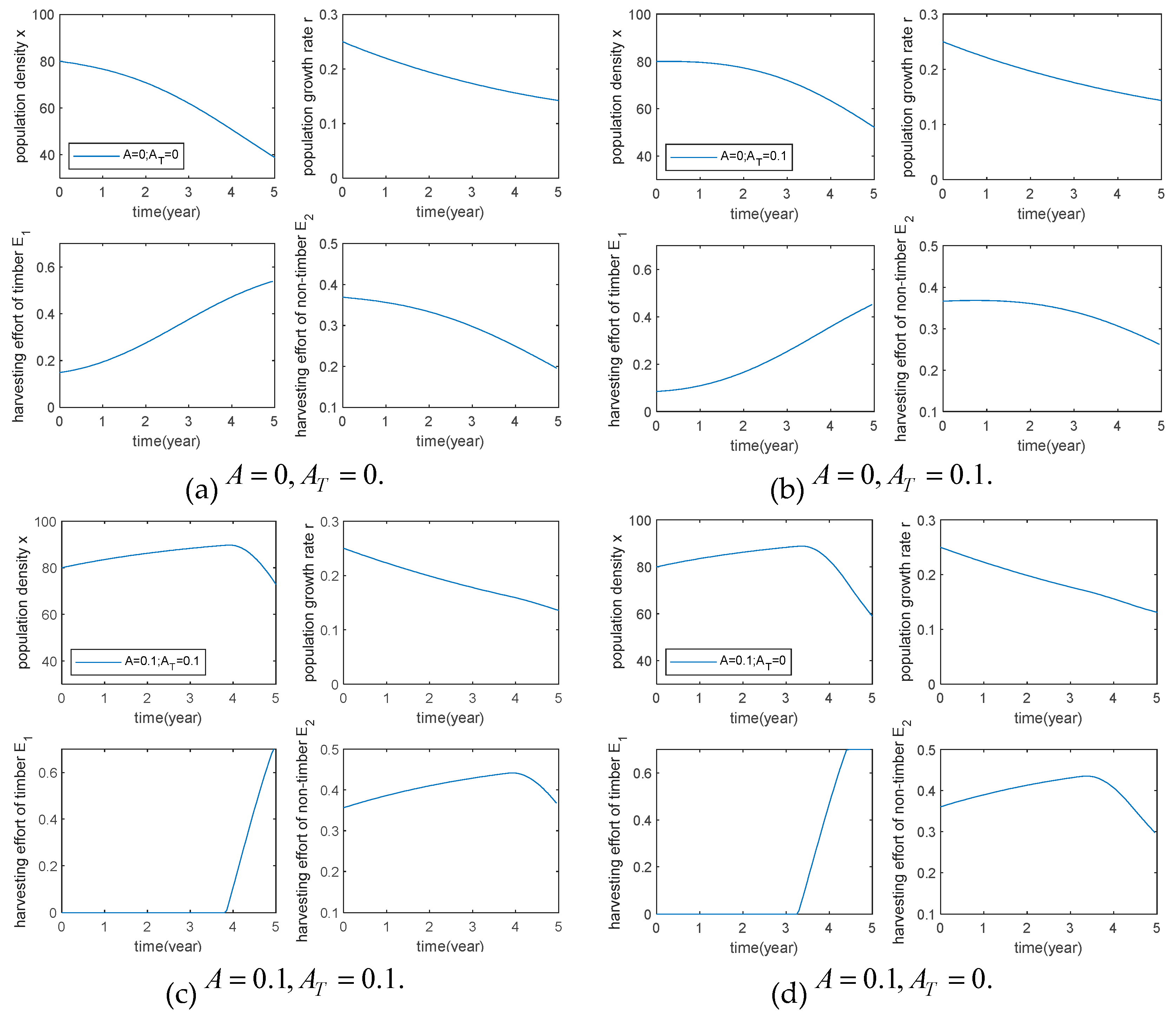
4.The importance of species conservation, and the influence of the importance of species conservation at the end of harvest on the optimal control strategy, some parameters are taken as

T = 5, τ = 5, r_{e} = 0.25, a = 0.01

,see Table 1 for other parameters.

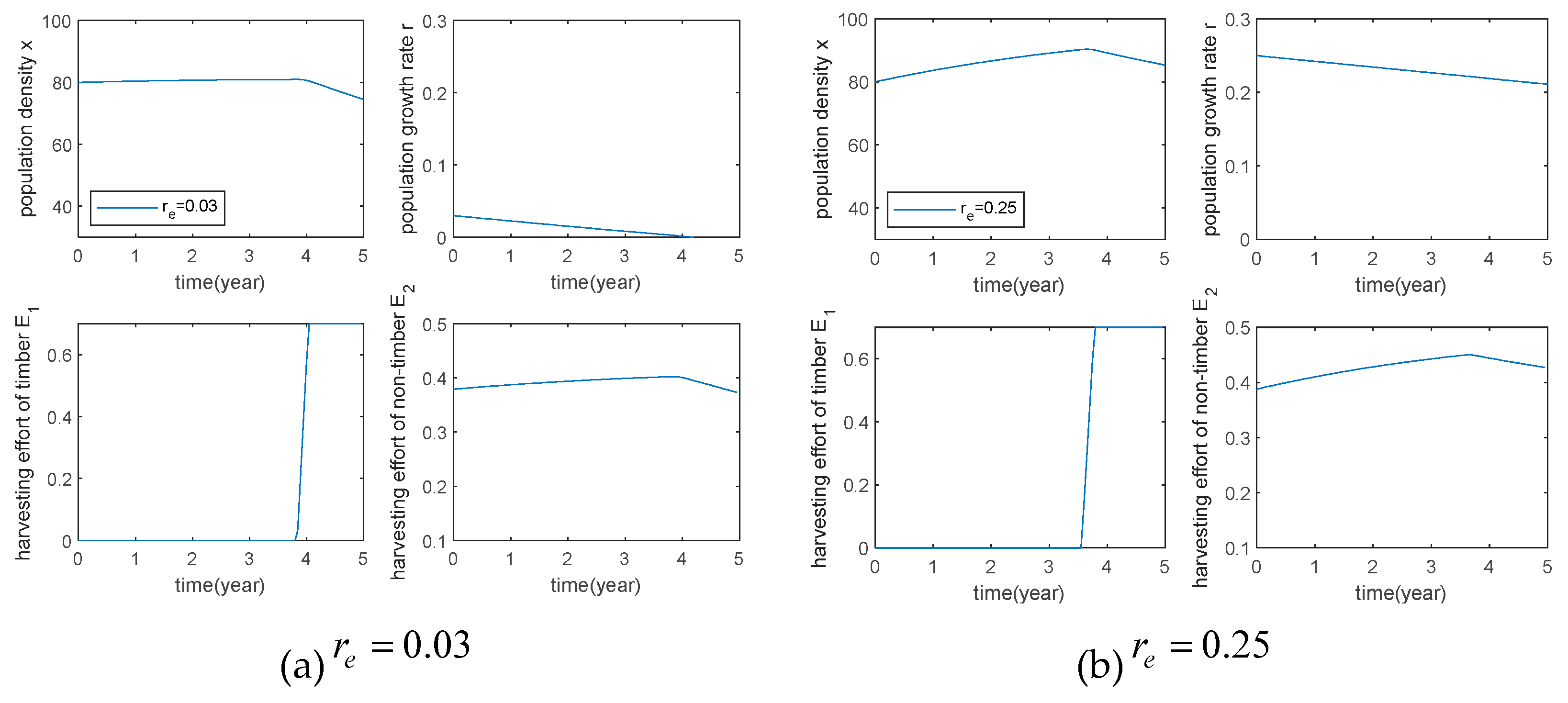
By comparing (b) with (c) in Figure 7, we shows that species with low importance of species conservation during harvest, which can be harvested from the beginning and the harvesting behavior is maintained until the end of the harvest, can obtain higher benefits. Species with lower importance of species conservation at the end of the harvest, higher harvest effort and lower population size at the end of the harvest also resulted in higher benefits.

4. Conclusion

In this paper, a combined timber and non-timber harvesting model with a nonlinear harvesting term was developed and the dynamical behavior of the model was investigated. It was concluded that when the combined harvesting was carried out, there existed a unique locally asymptotically stable positive equilibrium point in equation (2) when the condition was satisfied, and the plant growth rate was sustainable at that time for both timber and non-timber harvesting. When, there is only one trivial equilibrium point in equation (2), and harvesting timber and non-timber will result in a large decay rate of the plant population, which will eventually lead to extinction if the plant population keeps growing at such a growth rate.

For the optimal control problem of combined timber and non-timber harvesting with nonlinear harvesting, expression (5) of the optimal control strategy was obtained using the Hamilitonian function and Pontryagin’s optimality principle, and numerical simulations were carried out using MATLAB. The optimal harvesting strategy with nonlinear harvesting term can lead to higher ecological benefits and more sustainable development of the population.The price and cost of non-timber have a great impact on the harvesting benefits, so the combined harvesting of timber and non-timber can obtain more economic and ecological benefits.The timber treatment time, growth rate, and the importance of species conservation have a greater impact on the harvesting strategy. timber life span had almost no effect on the optimal harvesting strategy.

The combined timber and non-timber harvesting strategy with a nonlinear harvesting term can ensure higher ecological benefits while maximizing economic benefits, and provide a theoretical basis for the sustainable development of forestry ecology and economy.

Author Contributions

Conceptualization L.H.and S.H.;writing—original draft preparation Y.Z., L.H., and S.H.;Conceptualization,L.H., S.H. and Y.Z.:software,Y.Z.;data curation,Y.Z.validation L.H., S.H. and Y.Z. All authors have read and agreed to the published version of the manuscrip.

Funding

This work was supported by the National Natural Science Foundation of China (Program No. 11126239, No.11301036, No. 1140011471), and by Jilin provincial education department “13th Five-Year planning” (No. JJKH20200645KJ，No. JJKH20220662KJ).

Data Availability Statement

The data used to support the findings of this study are available from the corresponding author upon request.

Conflicts of Interest

The authors have no relevant financial or non-financial interests to disclose.

References

Liu, X.X. Dynamics analysis and harvesting strategy of predation system. Jilin University,Changchun,CHINA,2019.
Chen, X.F. Harvesting of a Prey-predator fisher based on leslie-gaower model. Journal of mathmatical Study, 2010, 3(3): 256-263.
Cheng, H.D.; Yin, Z.Y.; Liu, H.X. Analysis of the dynamic of stage-structured pest control model. Mathmatica Applicata, 2012, 25(4): 816-823.
Sudhakar, Y.; Vivek, K. A prey-predator model and control of a nematodes pest using control in banana:Mathematical modeling and qualitative analysis. International Journal of Biomathematics, 2022,15(1): 1-31.
Lv, Y.; Yuan, R.; Pei, Y. Dynamics in two nonsmooth predator-prey models with threshold Harvesting. Nonlinear Dynamics, 2013, 74(2): 107-132.
Mesterton-Gibbons, M. On the optimal policy for combining harvesting of predator and prey. Natural Resource Modeling. 1988, 3(1): 63-90. [CrossRef]
Yang, J.; Luan, X.F. Ecological impacts of non-timber forest product use. Chinese Journal of Applied Ecology, 2011, 22(3): 800－809.
Schmidt I, Mandle L, Ticktin,T, et al.What do matrix population model sreveal about the sustainability of non-timber forest product harvest ?. Journal of Applied Ecology, 2011,48: 815–826.
Gaoue O.G.; Ngonghala C.; Jiang J.; et al. Towards a mechanistic understanding of the synergistic effects of harvesting timber and non-timber forest products. Method in Ecology and Evolution, 2016, 7: 398-406. [CrossRef]
Yu, X.; Chen, F.; Lai, L. Dynamic behaviors of may type cooperative system with micha-elismenten type harvesting. Annals of Applied Mathematics, 2019, 35(4): 374-391.
Heggerud, C.M.; Lan, K.Q. Local stability analysis of ratio-dependent predator–prey models with predator harvesting rates. Applied Mathematics and Computation, 2015, 270: 349-357.
Zhang D.X; Sun G.; Xu M.L; et al. Spatial Dynamic Predator-Prey System with Time Delay and Nonlinear Harvesting Effect.Journal of Jilin University(ScienceEdition), 2018,56(3):515-522.
Agnew, T.T. Optimal exploitation of a fishery employ inganon-linear harvesting function. Ecological Modelling, 1979, 6: 47-57.
Gaoue O.G;Jiang J.; Ding W.; et al. Optimal harvesting strategies for timber and non-timber forest products in tropical ecosystems. Theoretical Ecology, 2016, 9: 287-297. [CrossRef]
Gaoue, O.G; Ticktin, T. Fulani knowledge of the ecologicalimpacts of Khaya senegalensis (Meliaceae) foliage harvest in Benin and its implications for sustainable harvest. Economic Botany, 2009, 63(3): 256–270.
Lande, R.; Engen, S.; Saether, B.E. Optimal harvesting economic discounting and extinction risk in fluctuat-ing populations. Nature, 1994, 372(6501): 88–90.
Armsworth, P.R.; Block, B.A.; Eagle, J.; Roughgarden, J.E. The role of discounting and dynamics in determ-ining the economic efficiency of time-area closures for managing fishery bycatch[J]. Theoretical Ecology, 2011, 4(4): 513–526.
Ticktin T.; Nantel P.; Ramirez F.;et al. Effects of variation on harvest limits for nontimber forest speci-es in Mexico. Conservation Biology, 2002, 16(3): 691–705.

Figure 1. Optimal solution with proportional harvesting.

Figure 2. Optimal solution with nonlinear harvesting.

Figure 3. Sensitivity analysis of the objective value

J

Figure 3. Sensitivity analysis of the objective value

J

Figure 4. Effect of optimal harvest for different timber treatment times.

Figure 5. Effect of optimal harvest for fast growth species and slow growth species.

Figure 6. Effect of optimal harvest for short and long-lived species.

Figure 7. Effect of optimal harvest for conservation weight coefficient

A

and conservation weight coefficient at the end of the harvest

A_{T}

Figure 7. Effect of optimal harvest for conservation weight coefficient

A

and conservation weight coefficient at the end of the harvest

A_{T}

Table 1. Notation for the model and optimal control and value.

	Values	Definition	References
$x_{0}$	80	Initial population density at $t = 0$	[14]
$K$	100	Carrying capacity for the plant	[14]
$r_{e}$	0.03,0.25	Maximum growth rate without harvest	[17,18]
$τ$	1,5,10,20	Average lifespan of the plant in years	Estimated
$α$	0.4	Growth decay rate for non-timber harvest	[15]
$β$	0.23	Growth decay rate due to timber harvest	[16]
$A$	0,0.1	Weight for the value of conservation	[14]
$A_{T}$	0,0.1	Weight for the value of conservation at the end of harvest	[14]
$δ$	0.05	Discount rate	[14]
$B_{1}$	0.3	Benefit from timber harvest	[14]
$B_{2}$	0.15	Benefit from non-timber harvest	[14]
$C_{1}$	15	Cost coefficient of timber harvesting	[14]
$C_{2}$	15	Cost coefficient of non-timber harvest	[14]
$a$	0.01,01	processing time for timber harvesting	Estimated
$M_{1}$	0.7	Upper bound for timber harvest rate	[14]
$M_{2}$	1	Upper bound for non-timber harvest rate	[14]

Disclaimer/Publisher’s Note: The statements, opinions and data contained in all publications are solely those of the individual author(s) and contributor(s) and not of MDPI and/or the editor(s). MDPI and/or the editor(s) disclaim responsibility for any injury to people or property resulting from any ideas, methods, instructions or products referred to in the content.

© 2024 by the authors. Licensee MDPI, Basel, Switzerland. This article is an open access article distributed under the terms and conditions of the Creative Commons Attribution (CC BY) license (http://creativecommons.org/licenses/by/4.0/).

Copyright: This open access article is published under a Creative Commons CC BY 4.0 license, which permit the free download, distribution, and reuse, provided that the author and preprint are cited in any reuse.

Alerts

MDPI Initiatives

Important Links

Choose an area of interest and we will send you notifications of new preprints at your preferred frequency.

Disclaimer

Optimal Harvesting Strategies for Timber and Non-timber Forest Products with Nonlinear Harvesting Term

Abstract

Keywords:

Subject:

0. Introduction

1. Model Building

2. Qualitative Analysis

2.1. Existence of Equilibrium Point

2.2. Stability of Equilibrium Point

3. Optimal Harvesting Strategy

4. Numerical Simulation

5.1. The Effect of Proportional Harvesting and Nonlinear Harvesting on the Optimal Harvesting Strategy

5.2. Sensitivity Analysis of Parameters

5.3. Effect of Different Parameters on the Optimal Harvesting Strategy

4. Conclusion

Author Contributions

Funding

Data Availability Statement

Conflicts of Interest

References

MDPI Initiatives

Important Links

Subscribe