Preprint
Article

DeClEx-Processing Pipeline for Critical Healthcare Application

Altmetrics

Downloads

83

Views

71

Comments

0

Submitted:

14 May 2024

Posted:

14 May 2024

You are already at the latest version

Alerts
Abstract
Over the last decade, the prevalence of health issues has increased by approximately 29.1%, putting a substantial strain on healthcare services. This has accelerated the integration of machine learning in healthcare, particularly following the COVID-19 pandemic. The utilization of machine learning in healthcare has grown significantly, however many present approaches are unsuitable for real-world implementation due to high memory footprints and lack of interpretability. We introduce DeClEx, a pipeline designed to address these issues. DeClEx ensures that data mirrors real-world settings by incorporating gaussian noise and blur and employing autoencoders to learn intermediate feature representations. Subsequently, our convolutional neural network, paired with spatial attention, provides comparable accuracy to state of the art pre-trained models while achieving threefold improvement in training speed. Furthermore, we provide interpretable results using explainable AI techniques. We integrate denoising and deblurring, classification and explainability in a single pipeline called DeClEx.
Keywords: 
Subject: Computer Science and Mathematics  -   Artificial Intelligence and Machine Learning

1. Introduction

Healthcare is the systematic provision of medical care to individuals by trained professionals with the objective to keep them healthy. The healthcare sector is divided into two categories: general healthcare and critical healthcare. General healthcare includes preventative screenings, periodic examinations, vaccines, and dental treatment. Recently, artificial intelligence (AI) has been utilized to streamline patient data management and provide appropriate treatment options. Critical healthcare involves acute medical treatments such as emergency services, intensive care, and surgical procedures. AI is applied vastly in this sector for patient monitoring and quicker decision making under time-constrained situations. In recent years, machine learning (ML) has been used to perform several tasks in healthcare and biomedicine. These techniques are used for anomaly detection, predictive analytics, drug discovery and development, genetic mutation analysis, gene expression analysis, personal health monitoring, and disease spread modeling. Nanyue et al. [1] utilized principal component analysis (PCA) and least squares (LS) to analyze and differentiate pulse-diagnosis signals between patients with fatty liver disease and Cirrhosis, aiming to aid in TCM diagnosis. Kim et al. [2] used support vector machines (SVM), random forest, artificial neural networks (ANN) to identify risk of osteoporosis in postmenopausal women. Seixas et al. [3] employed k-nearest neighbors (KNN), decision tree, multi-layer perceptron (MLP) and naïve-bayes for segmentation and pattern recognition of lower limb skin ulcers in medical images. Tulder and Bruijne [4] studied the use of convolutional classification restricted boltzmann machines to help with feature learning of lung texture classification and airway detection in CT images. Gerazov and Conceicao [5] made use of a deep convolutional neural network (DCNN) for tumor classification in homogeneous breast tissue. Tyagi, Mehra, and Saxena [6] adopted SVM and KNN for accurately predicting thyroid disease. Anastasiou et al. [7] proposed MODELHealth to process and anonymize health data using ML architectures. Tsarapatsani et al. [8] applied extreme grading boosting (XGB) and adaptive boosting (AdaBoost) for cardiovascular disease prediction. Sabir et al. [9] leveraged ResUNet to segment liver tumors from CT scans. Recent trends also show increased use of contrastive learning methods in medical care [10,11]. In the past few years, explainable AI methods have turned opaque, “black box” models into transparent, “white box” models, allowing both experts and beginners to gain an in-depth understanding of the reasoning behind certain predictions. This approach has been extensively applied in healthcare, providing clinicians with crucial decision-making support. Workman et al. [12] provided explainability using impact scores for each feature within a deep learning model aimed at understanding opioid use disorder. Hossain, Muhammad and Guizani [13] integrated local interpretable model-agnostic explanations (LIME) in a healthcare framework to combat COVID 19-like pandemics. Marvin and Alam [14] utilized LIME, shapley additive explanations (SHAP) to highlight feature importances in neonatal intensive care unit (NICU). Ammar et al. [15] proposed an explainable multimodal AI platform called SPACES for active surveillance, diagnosis, and management of adverse childhood experiences (ACEs). She et al. [16] investigated a web-based explainable AI screening for prolonged grief disorder. [17] and [18] applied interpretable AI techniques for maternal health risk prediction and empowering glioma prognosis respectively.

2. Proposed Method

Dedicated autoencoders are used to process noisy and blur images. Then we make predictions using 3 different models and select the best model to provide explainability. Figure 1 illustrates the entire process.

2.1. Dataset

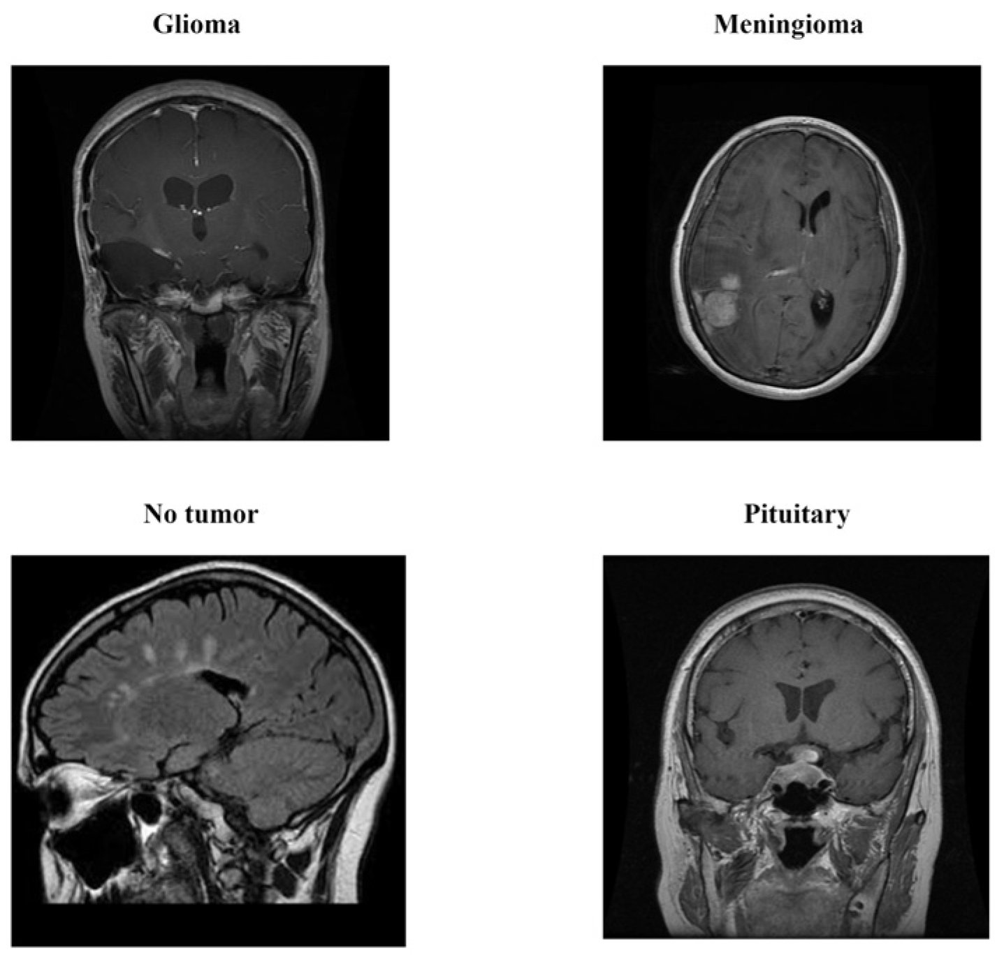
The original data provided in this study is openly available at https://www.kaggle.com/datasets/masoudnickparvar/brain-tumor-mri-dataset. This data contains MRI scans of the brain, categorized into Glioma, Meningioma, Pituitary, or No tumor. It includes 7022 images, comprising 1623 Glioma, 1647 Meningioma, 2002 No tumor, and 1750 Pituitary scans. Figure 2 depicts sample images across all four classes.

2.2. Implementation of Pre-Trained Models for Comparison

Initially, we use pre-trained models on the data to come up with baseline findings for future comparison. We implement two models namely ResNet-50 and VGG-16 for classifying tumor images into one of the four mentioned classes. Initially, the data is processed by an image data generator, which performs several random translations to improve generalization. The dataset is then divided into 80% training and 20% testing. Next, we train ResNet-50 by freezing the base model’s layers, preventing their weights from updating. To prevent model overfitting dropout is used. We utilize softmax for probability distribution over classes, with categorical cross entropy as the loss function. We achieve a 97.86% test accuracy. Subsequently, VGG-16 is trained using an identical setup with the same activation function and loss function. We achieve a test accuracy of 81.01%. Therefore, we select the ResNet-50 model for benchmarking and comparative evaluation.

2.3. Noise and Blur Introduction

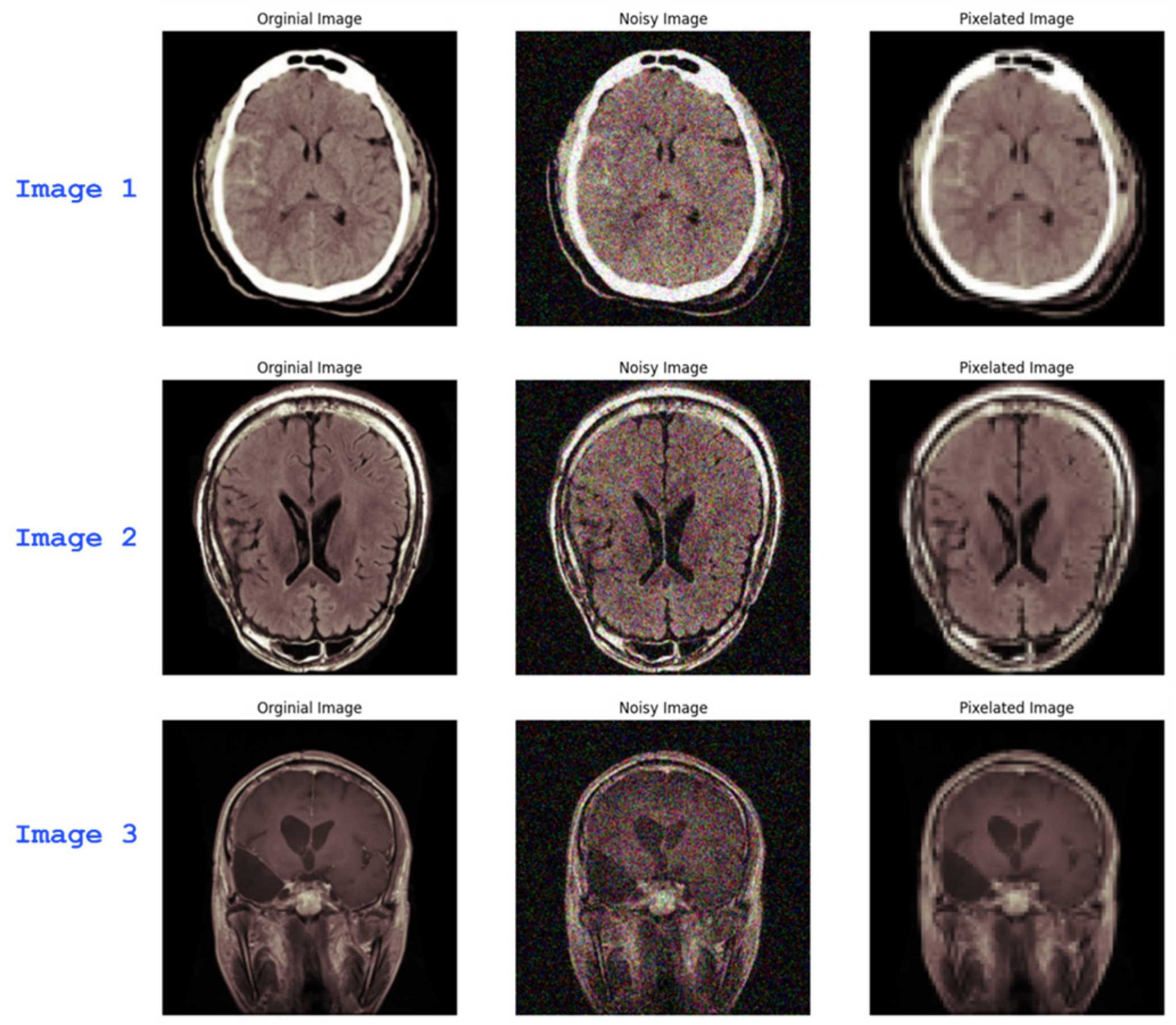
To improve the classification model’s generalization to real-world test data, we deliberately introduce noise and blur in our training set. Figure 3 shows original images alongside their noisy and blurred representations. Real-time test images often contain subtle noise that is unnoticeable to the human eye but has an adverse impact on model performance. Some images may also have low resolution. To help classification models later, we create a pipeline which intentionally pixelates the image first and then introduces noise. Following an in-depth literature survey, in which most studies across different tasks included 15% noise in their images, we add 15% noise in the data leaving the remainder unchanged.

2.3. Autoencoders for Noise and Blur Mitigation

An autoencoder consists of an encoder-decoder architecture. The encoder transforms the input into a latent-space representation, learning to preserve the data’s most important attributes. The decoder then reconstructs the input data using this compressed version. This not only helps with dimensionality reduction but also in learning efficient data encodings. Figure 4 represents a high level overview of an autoencoder.
Figure 4. Schematic representation of an Autoencoder [19].
Preprints 106443 g004
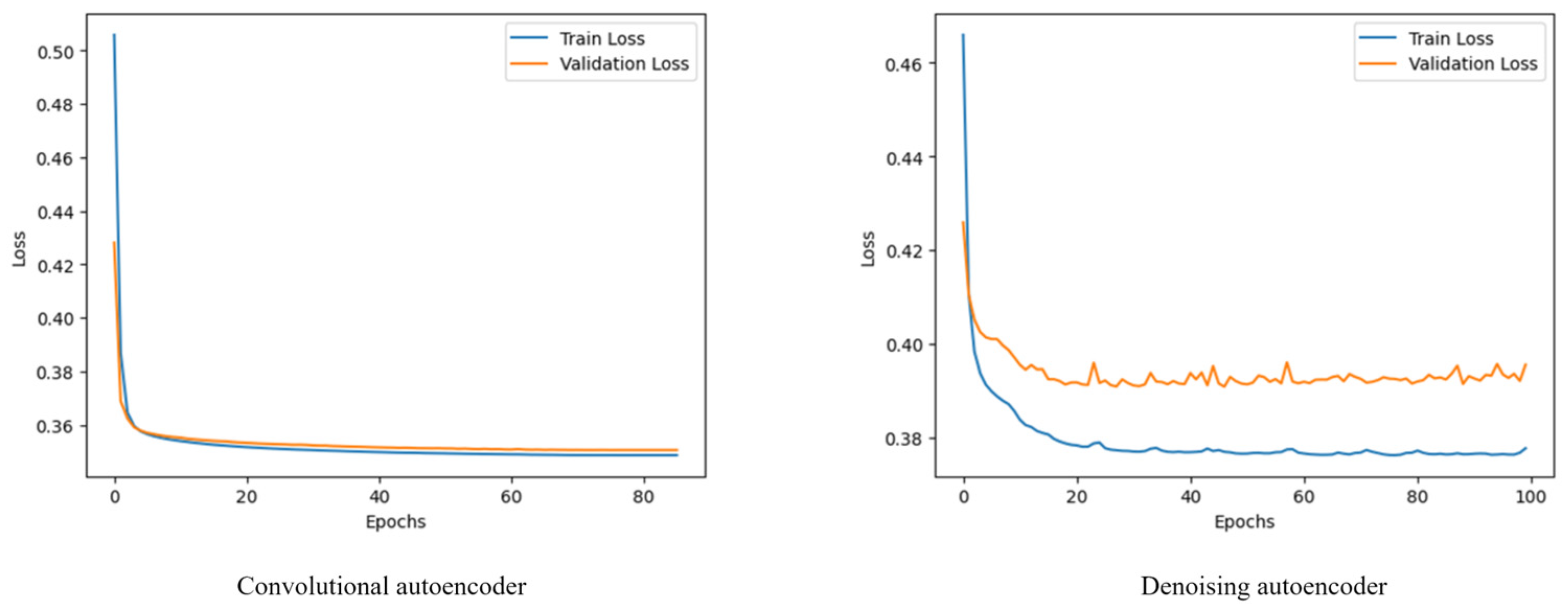
We experiment with convolutional and denoising autoencoders and then select the best model among these for our denoising task. For a convolutional autoencoder, the input is passed through a convolutional layer consisting of 32 filters. The activation function used is a rectified linear unit (ReLU) and we keep padding the same to preserve spatial dimensions. This is then followed by a max pooling layer. We add a dropout layer for regularization purposes. The decoder mirrors the encoder but in reverse and the activation function used in the last layer is sigmoid. A denoising autoencoder consists of a dense architecture with fully connected layers. The data is first transformed by dense layers using ReLU as the activation function and subsequently decoded by dense layers having Sigmoid activation. Convolutional autoencoders perform better and hence we use this for the denoising task. Figure 5 and Figure S2 prove this quantitatively and qualitatively respectively.
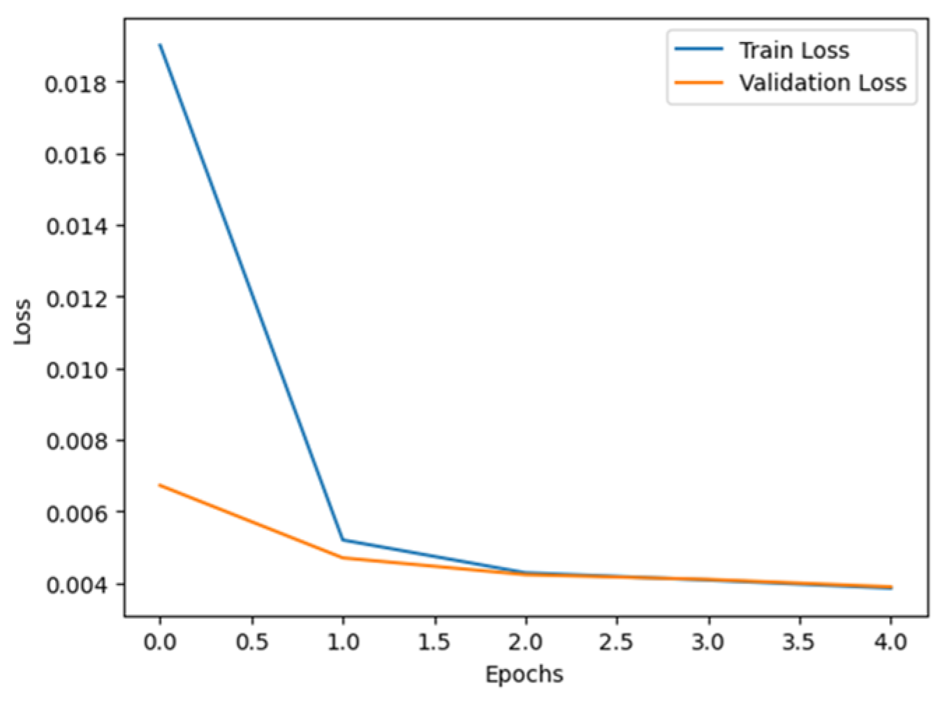
We first scale down the image by 20% and then resize it back to obtain the pixelated effect. Then we train an autoencoder with successive convolution layers to learn hidden feature representation and de-blur the images. The final layer outputs a three-channel image while maintaining the original color depth. Figure 6 shows the loss curve for deblurring autoencoder.

2.3. Noise Ablation Study

We conduct a noise ablation study to explore autoencoders’ resilience to noise during testing. This involves intentionally adding increasing degrees of noise, specifically 15%, 20%, and 30% into the training data using noise perturbation methods. By doing so, we hope to see if training autoencoders with such distortions improves the ability to reconstruct data properly when faced with similar noise patterns during testing. This method aids in determining the model’s noise resistance and practical applicability in situations when data corruption is possible. We add gaussian noise into our data during train as well as test time. Gaussian noise, also known as normal noise, is a type of statistical noise that has the same probability density function as the normal distribution. This is an effective representation of random noise that may be found in both natural and man-made systems. Gaussian distribution is defined by a bell-shaped curve symmetrical around the mean value. Adding gaussian noise to data during training can make machine learning models more resilient to unexpected inputs in real-world scenarios. This method not only assesses models’ robustness in noisy environments, but also improves their capacity to generalize.

3. Results

With our pipeline, we first add noise to the training dataset, allowing autoencoders to reconstruct the data. This approach has proven effective in a wide range of applications, from simple image classification to complex time-series regression problems. Chen, Hong, and Zhou [20] introduced noise to estimate the capacity degradation over time using an autoencoder followed by a transformer encoder architecture.
First, we aim to evaluate ResNet-50 which we previously identified as our best model. We perform ablation study on a noisy test set using both a stand alone ResNet-50 and a combination of autoencoder and ResNet-50. Our findings detailed in Table 1 indicate that integrating autoencoders with ResNet-50 enhances performance in noisy environments.
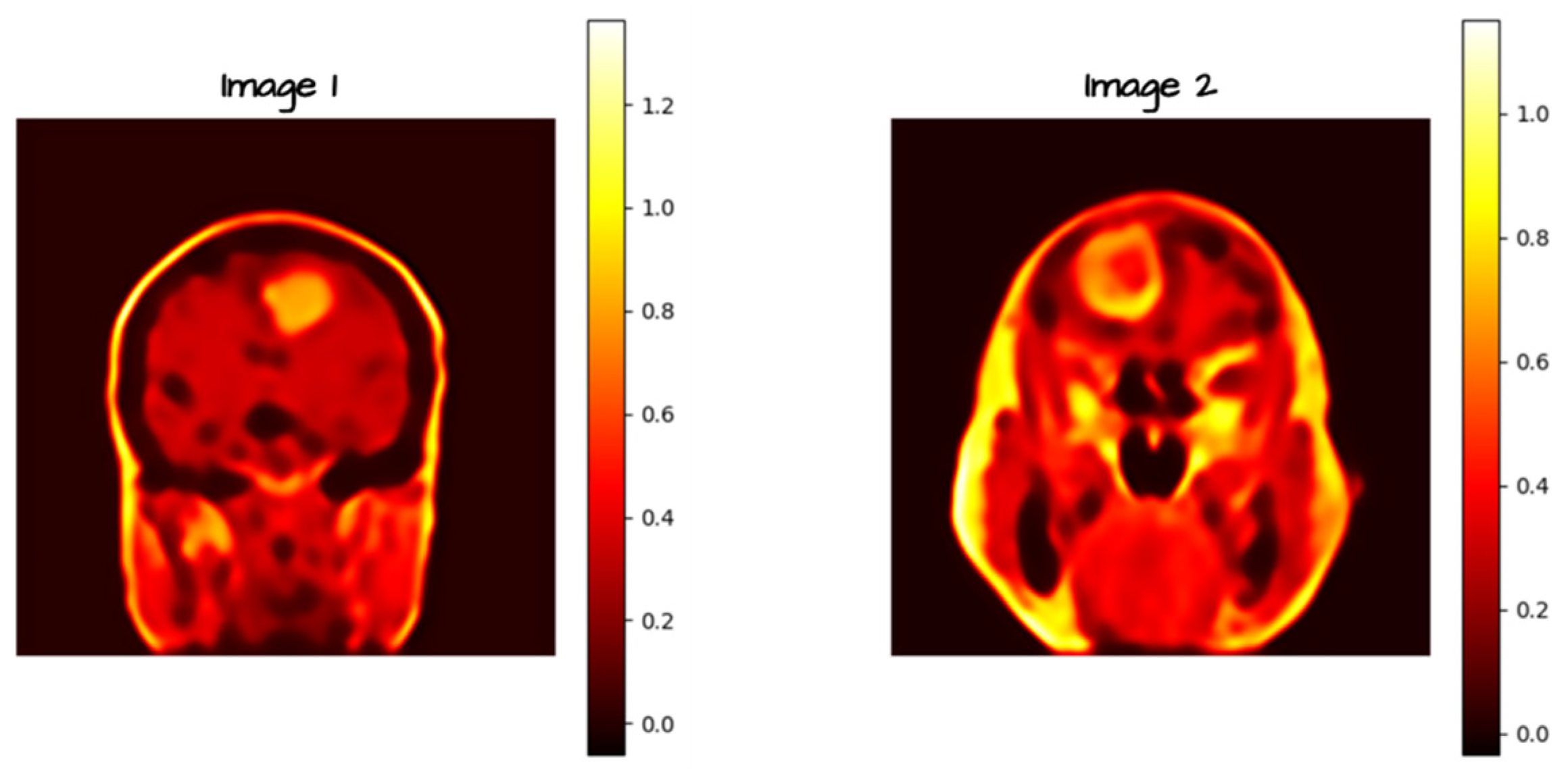
We then implement a CNN with spatial attention for the classification task. This architecture significantly reduces the number of parameters, maintains comparable accuracy, and achieves a threefold increase in training speed relative to ResNet-50. Spatial attention is a technique that improves performance of neural nets for image classification and detection tasks. This method directs the model’s attention to specific parts of the image, prioritizing informative feature regions over non-informative ones. It generates a spatial feature map (Figure 7) by concatenating features obtained through average and max pooling. This is passed through a sigmoid function which normalizes the values between 0 and 1. The values closer to 1 are considered more important.
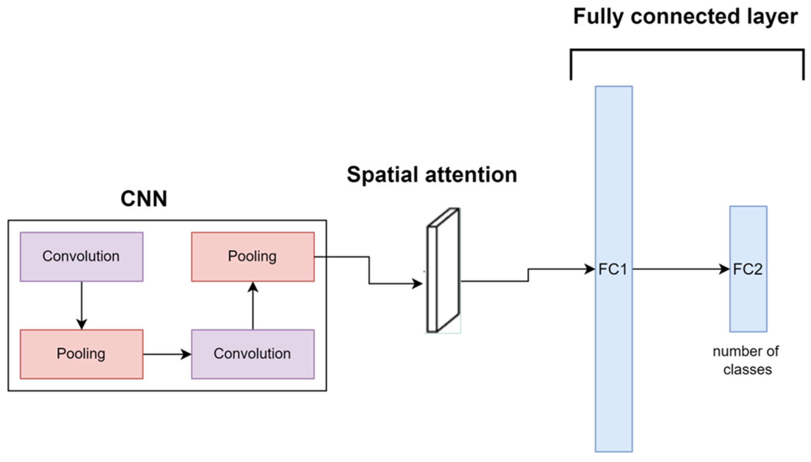
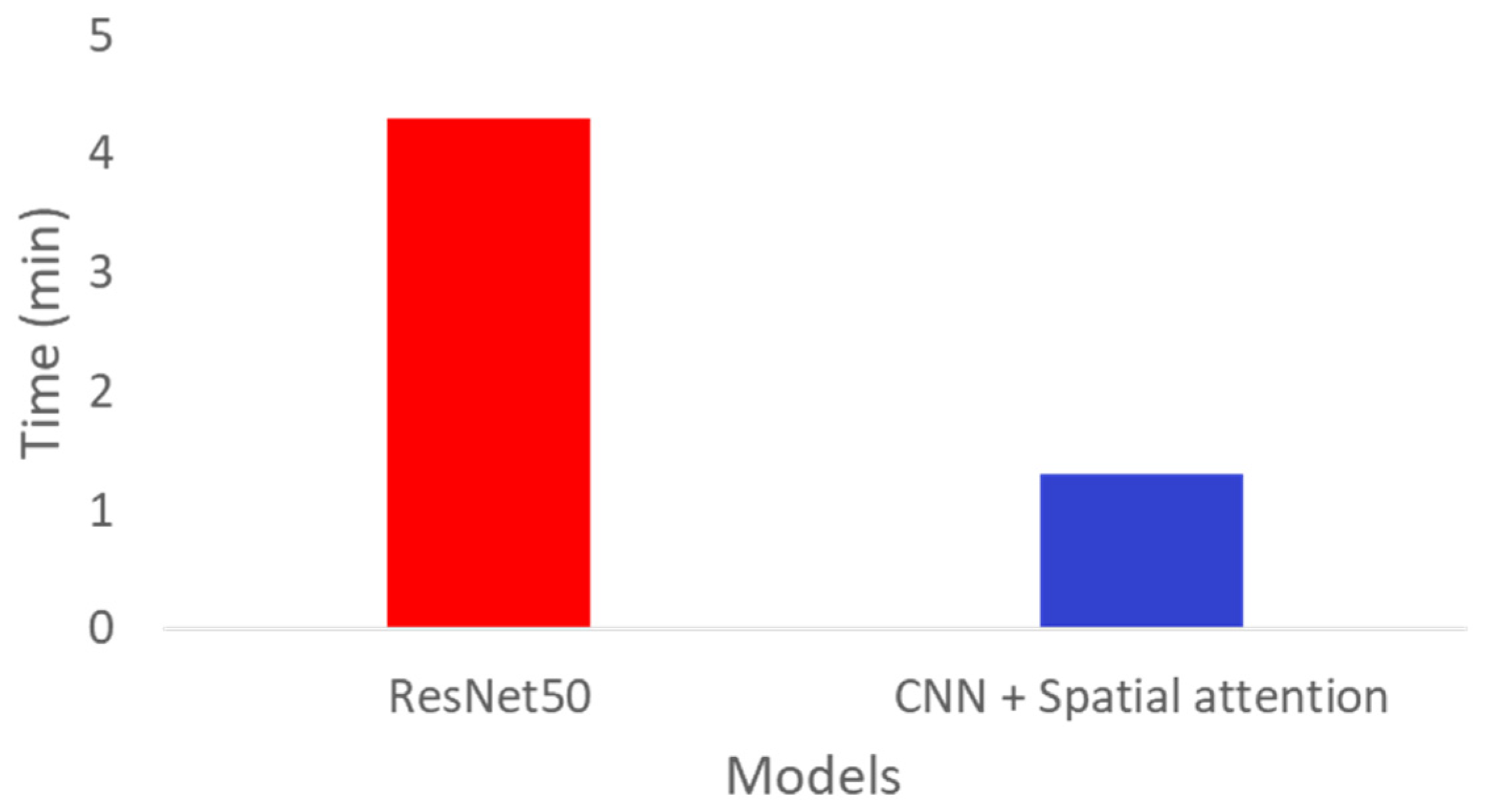
In this architecture (Figure 8 and Figure 9), the images first pass through alternating convolution layers and max pooling layers to capture spatial hierarchies and reduce dimensionality. Subsequently we pass it through a spatial attention module followed by dense layers to obtain classification results. Experiments are run on a system using Python 3.10, Tensorflow 2.0 and Keras with Nvidia A100 and Nvidia T4 GPUs. We obtain a 93.13% accuracy on the test set, comparable to ResNet-50. Consequently, we replace ResNet-50 with CNN + spatial attention as our optimal model due to its faster training time as shown in Figure 10.
Figure 8. Spatial attention module [21].
Preprints 106443 g008
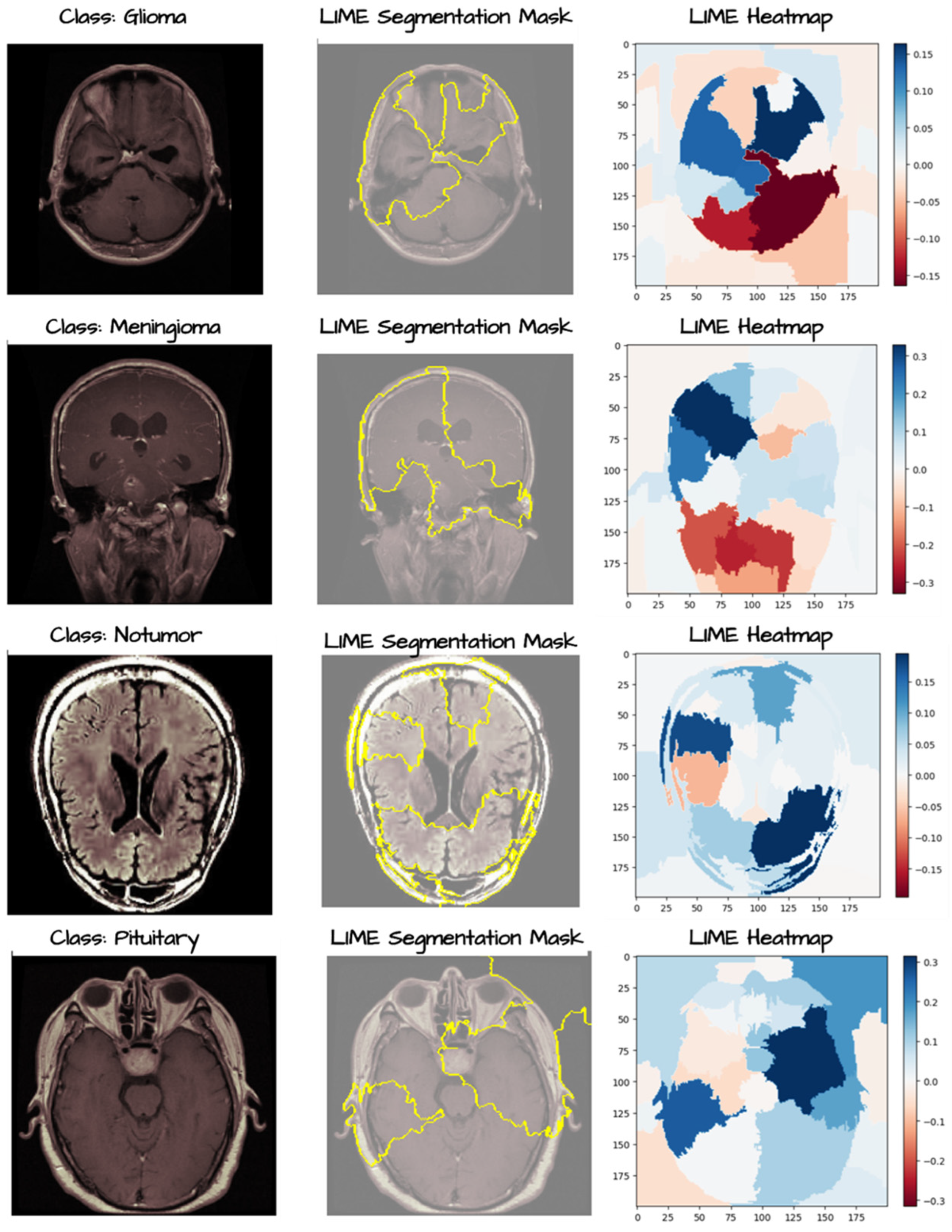
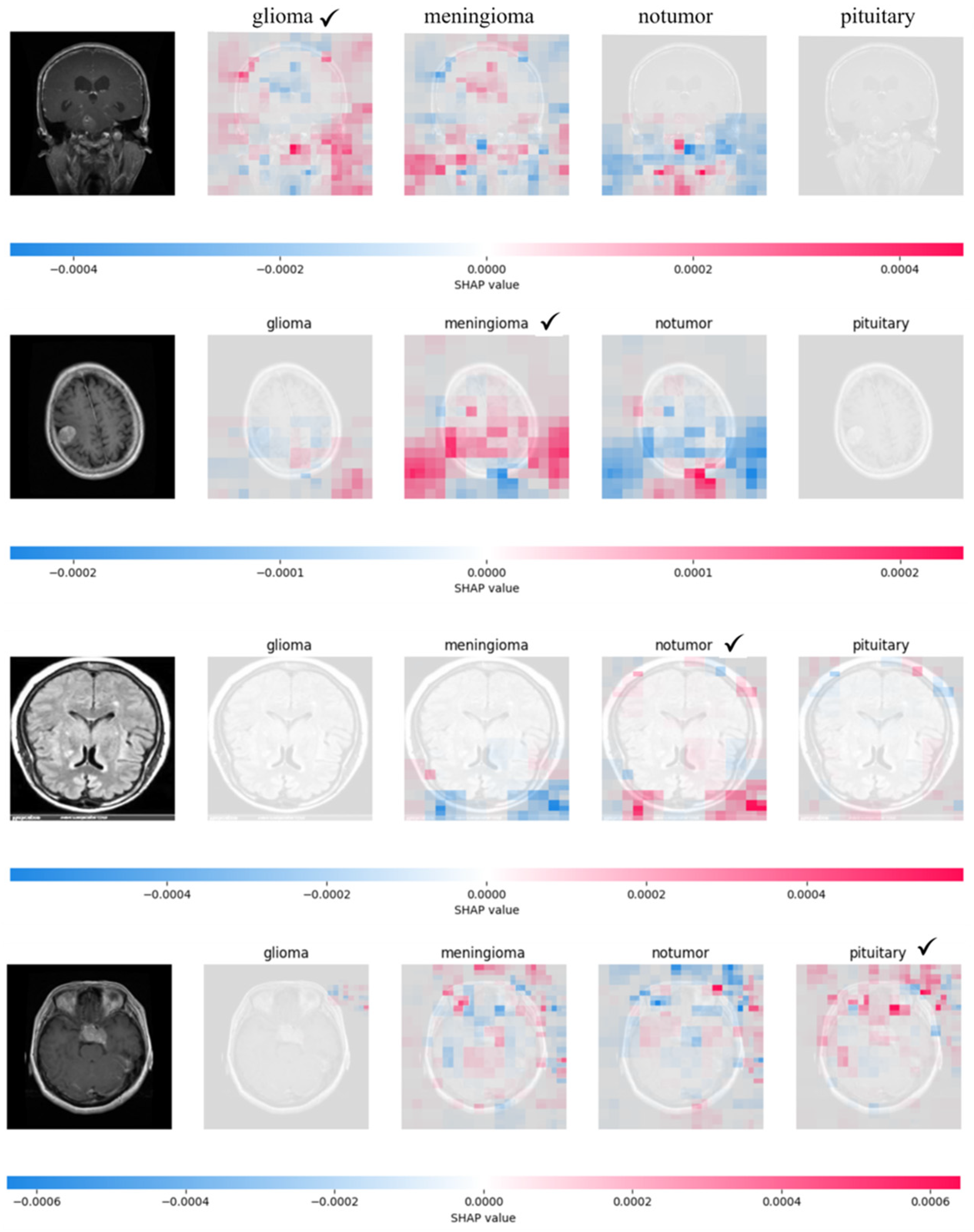
Next, we utilize Explainable AI (XAI) techniques, specifically Local Interpretable Model-Agnostic Explanations (LIME) and Shapley Additive Explanations (SHAP), to transform the black box CNN with spatial attention into a transparent model. XAI is crucial in healthcare since decisions that have life-changing repercussions must be clear. The use of XAI allows healthcare professionals to interpret AI generated diagnosis and treatment plans. Ribeiro, Singh, and Guestrin [22] proposed LIME to explain the decisions of any classifier. LIME achieves this by zooming into the local area of interest. This area is analyzed in depth to gain insights. LIME fits a sparse linear model from a set of linear interpretable models in the local area. Lundenberg and Lee [23] proposed SHAP to interpret complex ML models. SHAP values are used to ascertain the importance of individual pixels in brain MRI scans. A ML model is utilized to make a prediction. Then a baseline image is selected. Pixels of this image are altered to evaluate single pixel and multiple pixel change impact on model’s prediction. Shapley values are calculated according to the contribution across all possible combinations. Higher Shapley values indicate a higher pixel importance. Figure 11 and Figure 12 depict the results for LIME and SHAP across all four classes.

4. Discussion

The study demonstrates the effectiveness of our proposed pipeline for tumor classification from brain MRI scans. Our comprehensive approach enhances interpretability for diagnostic imaging applications. However, there are additional areas we aim to explore in future research. Large Language Models (LLMs) such as GPT [24], Llama [25] and MedPaLM [26] have been the talk of the town in recent years and have received significant attention from both industry as well as academia. LLMs have been used for a wide range of tasks from creating human-like language, generating sophisticated code and engaging in nuanced dialogues. We plan on using LLMs for precise tumor classification in brain MRI scans, as well as providing detailed explanatory narratives. This will streamline the current three-step diagnostic process into a single step. We plan to integrate retrieval augmented generation (RAG) [27] in our framework in such a way that once the pipeline gets executed, clinicians can ask relevant medical questions and the RAG model can give informed answers to these questions. This integration will lead to even better decision support. We also aim to explore various adversarial attacks and defense mechanisms [28] in future. Integrating all of the above components can lead to better treatment plans.

5. Conclusions

We propose a pipeline which 1. improves model resilience to real-world data by including noise and blur in the train set and using autoencoders to learn data representations from these altered inputs. Furthermore, 2. We demonstrate that CNN with spatial attention not only equals the performance of state-of-the-art pretrained models, but does so with a threefold improvement in training speed. The spatial attention component successfully captures subtle spatial information in MRI scans. 3. We also examine explainable AI techniques to provide transparency in the decision making phase. 4. We implement this pipeline as a web application where clinicians can upload brain MRI scans and receive a comprehensive analysis of these images.

Supplementary Materials

The following supporting information can be downloaded at the website of this paper posted on Preprints.org, Figure S1: Train and validation accuracy curves for different noise levels. Figure S2: Qualitative evaluation of Convolutional and Denoising autoencoder. Figure S3: Qualitative evaluation of Deblurring autoencoder.

Author Contributions

GS and SCG conceptualized the project. PS, GS and SCG performed all the experiments. AH co-advised the project and helped shape the goal of the project.

Funding

This research received no funding.

Institutional Review Board Statement

Not applicable.

Conflicts of Interest

The authors declare no conflict of interest.

References

  1. Nanyue, W. et al. Comparative study of pulse-diagnosis signals between 2 kinds of liver disease patients based on the combination of unsupervised learning and supervised learning. 2013 IEEE International Conference on Bioinformatics and Biomedicine 2013, pp. 260-262. [Online]. [CrossRef]
  2. Kim, S. K., Yoo, T. K., Oh, E., & Kim, D. W. Osteoporosis risk prediction using machine learning and conventional methods. Annual International Conference of the IEEE Engineering in Medicine and Biology Society 2013, pp. 188-191. [Online]. [CrossRef]
  3. Seixas, J. L., Barbon, S., & Mantovani, R. G. Pattern Recognition of Lower Member Skin Ulcers in Medical Images with Machine Learning Algorithms. 2015 IEEE 28th International Symposium on Computer-Based Medical Systems 2015, pp. 50-53. [Online]. [CrossRef]
  4. van Tulder, G. & de Bruijne, M. Combining Generative and Discriminative Representation Learning for Lung CT Analysis With Convolutional Restricted Boltzmann Machines. IEEE Transactions on Medical Imaging 2016, 35(5), pp. 1262-1272. [Online]. [CrossRef]
  5. Gerazov, B. & Conceicao, R. C. Deep learning for tumour classification in homogeneous breast tissue in medical microwave imaging. IEEE EUROCON 2017 - 17th International Conference on Smart Technologies 2017, pp. 564-569. [Online]. [CrossRef]
  6. Tyagi, A., Mehra, R., & Saxena, A. Interactive Thyroid Disease Prediction System Using Machine Learning Technique. 2018 Fifth International Conference on Parallel, Distributed and Grid Computing (PDGC) 2018, pp. 689-693. [Online]. [CrossRef]
  7. Anastasiou, A., Pitoglou, S., Androutsou, T., Kostalas, E., Matsopoulos, G., & Koutsouris, D. MODELHealth: An Innovative Software Platform for Machine Learning in Healthcare Leveraging Indoor Localization Services. 2019 20th IEEE International Conference on Mobile Data Management (MDM) 2019, pp. 443-446. [Online]. [CrossRef]
  8. Tsarapatsani, K. et al. Machine Learning Models for Cardiovascular Disease Events Prediction. 2022 44th Annual International Conference of the IEEE Engineering in Medicine & Biology Society (EMBC) 2022, pp. 1066-1069. [Online]. [CrossRef]
  9. Sabir, M.W., Khan, Z., Saad, N.M., Khan, D.M., Al-Khasawneh, M.A., Perveen, K., Qayyum, A., & Ali, S.S. Azhar. Segmentation of Liver Tumor in CT Scan Using ResU-Net. Applied Sciences 2022, 12, 8650. [Online]. [CrossRef]
  10. Zhao, X., Fang, C., Fan, D.-J., Lin, X., Gao, F., & Li, G. Cross-Level Contrastive Learning and Consistency Constraint for Semi-Supervised Medical Image Segmentation. 2022 IEEE 19th International Symposium on Biomedical Imaging (ISBI) 2022, pp. 1-5. [Online]. [CrossRef]
  11. Li, X., Fan, Y., Zheng, H., Gao, J., Wei, X., & Yu, M. Balanced And Discriminative Contrastive Learning For Class-Imbalanced Medical Images. ICASSP 2024 - 2024 IEEE International Conference on Acoustics, Speech and Signal Processing (ICASSP) 2024, pp. 3735-3739. [Online. [CrossRef]
  12. Workman, T. E. et al. Explainable Deep Learning Applied to Understanding Opioid Use Disorder and Its Risk Factors. 2019 IEEE International Conference on Big Data (Big Data) 2019, pp. 4883-4888. [Online]. [CrossRef]
  13. Hossain, M. S., Muhammad, G., & Guizani, N. Explainable AI and Mass Surveillance System-Based Healthcare Framework to Combat COVID-19 Like Pandemics. IEEE Network 2020, 34(4), pp. 126-132, July/August. [Online]. [CrossRef]
  14. Marvin, G. & Alam, M. G. R. Explainable Feature Learning for Predicting Neonatal Intensive Care Unit (NICU) Admissions. 2021 IEEE International Conference on Biomedical Engineering, Computer and Information Technology for Health 2021, pp. 69-74. [Online]. [CrossRef]
  15. Ammar, N. et al. SPACES: Explainable Multimodal AI for Active Surveillance, Diagnosis, and Management of Adverse Childhood Experiences (ACEs). 2021 IEEE International Conference on Big Data (Big Data) 2021, pp. 5843-5847. [Online]. [CrossRef]
  16. She, W. J. et al. Investigation of a Web-Based Explainable AI Screening for Prolonged Grief Disorder. IEEE Access 2022, 10, pp. 41164-41185. [Online]. [CrossRef]
  17. Rahman, A. & Alam, M. G. Rabiul. Explainable AI-based Maternal Health Risk Prediction using Machine Learning and Deep Learning. 2023 IEEE World AI IoT Congress (AIIoT) 2023, pp. 0013-0018. [Online]. [CrossRef]
  18. Palkar, A., Dias, C. C., Chadaga, K., & Sampathila, N. Empowering Glioma Prognosis With Transparent Machine Learning and Interpretative Insights Using Explainable AI. IEEE Access 2024, 12, pp. 31697-31718. [Online]. [CrossRef]
  19. Shinde, G., Mohapatra, R., Krishan, P., Garg, H., Prabhu, S., Das, S., Masum, M., & Sengupta, S. The State of Lithium-Ion Battery Health Prognostics in the CPS Era. to be submitted.
  20. Chen, D., Hong, W., & Zhou, X. Transformer Network for Remaining Useful Life Prediction of Lithium-Ion Batteries. IEEE Access 2022, 10, pp. 19621-19628. [Online]. [CrossRef]
  21. Yu, J., Shen, Y., Liu, N., & Pan, Q. Frequency-Enhanced Channel-Spatial Attention Module for Grain Pests Classification. Agriculture 2022, 12, 2046. [Online]. [CrossRef]
  22. Ribeiro, M. T., Singh, S., & Guestrin, C. “Why Should I Trust You?”: Explaining the Predictions of Any Classifier 2016. arXiv preprint. arXiv:1602.04938.
  23. Lundberg, S. & Lee, S.-I. A Unified Approach to Interpreting Model Predictions 2017. arXiv preprint. arXiv:1705.07874.
  24. Radford, A. & Narasimhan, K. Improving Language Understanding by Generative Pre-Training 2018.
  25. Touvron, H., Lavril, T., Izacard, G., Martinet, X., Lachaux, M.-A., Lacroix, T., Rozière, B., Goyal, N., Hambro, E., Azhar, F., Rodriguez, A., Joulin, A., Grave, E., & Lample, G. LLaMA: Open and Efficient Foundation Language Models 2023. arXiv preprint. arXiv:2302.13971.
  26. Singhal, K., Azizi, S., Tu, T. et al. Large language models encode clinical knowledge. Nature 620, 172–180 2023. [CrossRef]
  27. Lewis, P., Perez, E., Piktus, A., Petroni, F., Karpukhin, V., Goyal, N., Küttler, H., Lewis, M., Yih, W.-t., Rocktäschel, T., Riedel, S., & Kiela, D. Retrieval-Augmented Generation for Knowledge-Intensive NLP Tasks 2021. arXiv preprint. arXiv:2005.11401.
  28. Chen, Y., Zhang, M., Li, J., & Kuang, X. Adversarial Attacks and Defenses in Image Classification: A Practical Perspective. 2022 7th International Conference on Image, Vision and Computing (ICIVC) 2022, pp. 424-430. [Online]. [CrossRef]
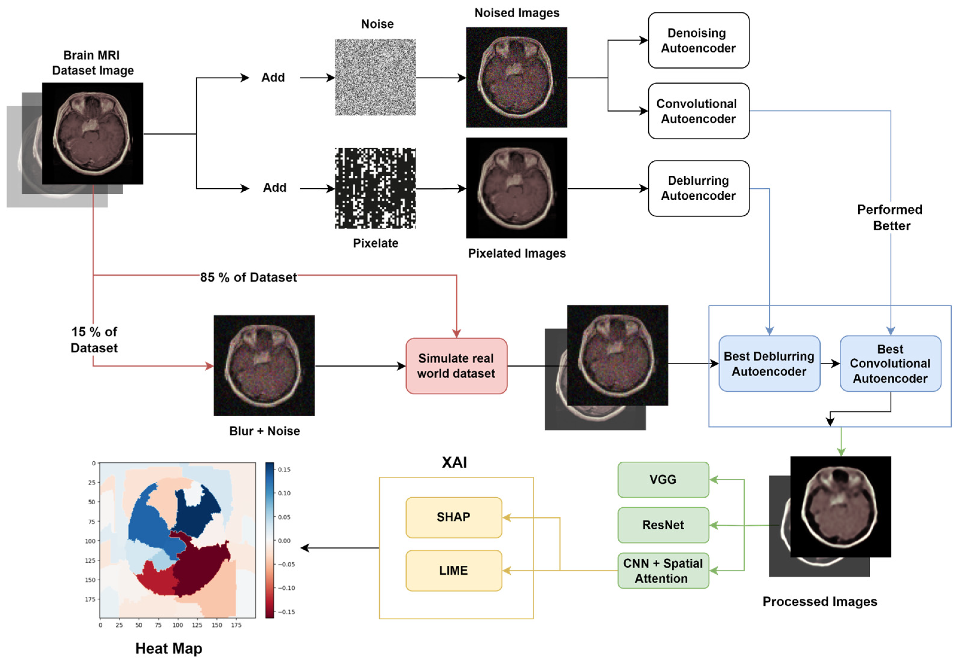
Figure 1. Proposed DeClEx Architecture.
Preprints 106443 g001
Figure 2. Samples of Classes in Data.
Preprints 106443 g002
Figure 3. Images along their noisy and blurred versions.
Preprints 106443 g003
Figure 5. Loss curves for Convolutional and Denoising Autoencoders.
Preprints 106443 g005
Figure 6. Loss curve for Deblurring Autoencoder.
Preprints 106443 g006
Figure 7. Concatenated feature maps for two image samples.
Preprints 106443 g007
Figure 9. CNN with Spatial Attention architecture.
Preprints 106443 g009
Figure 10. Train time for ResNet-50 and CNN + spatial attention.
Preprints 106443 g010
Figure 11. LIME segment masks and heat maps for all 4 classes.
Preprints 106443 g011
Figure 12. SHAP pixel value for all four classes.
Preprints 106443 g012
Table 1. Performance comparison on noisy data with and without Autoencoder.
Test accuracy (%)
Noise level (%) ResNet-50 Autoencoder + Resnet-50
15% 88.94% 94.51%
20% 81.69% 83.60%
30% 73.07% 77.96%
Disclaimer/Publisher’s Note: The statements, opinions and data contained in all publications are solely those of the individual author(s) and contributor(s) and not of MDPI and/or the editor(s). MDPI and/or the editor(s) disclaim responsibility for any injury to people or property resulting from any ideas, methods, instructions or products referred to in the content.
Copyright: This open access article is published under a Creative Commons CC BY 4.0 license, which permit the free download, distribution, and reuse, provided that the author and preprint are cited in any reuse.
Prerpints.org logo

Preprints.org is a free preprint server supported by MDPI in Basel, Switzerland.

Subscribe

© 2024 MDPI (Basel, Switzerland) unless otherwise stated