Submitted:
15 May 2024
Posted:
15 May 2024
You are already at the latest version
Abstract
Keywords:
1. Introduction
2. Materials and Methods
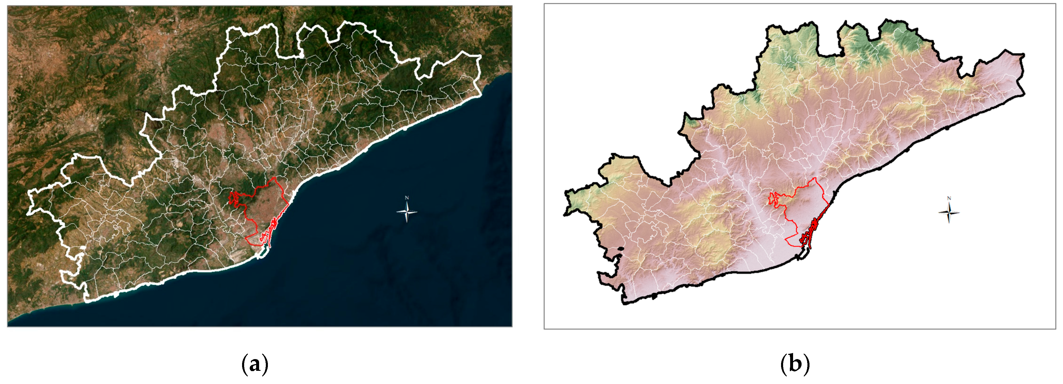
2.1. The Field of Study
2.2. Methodology
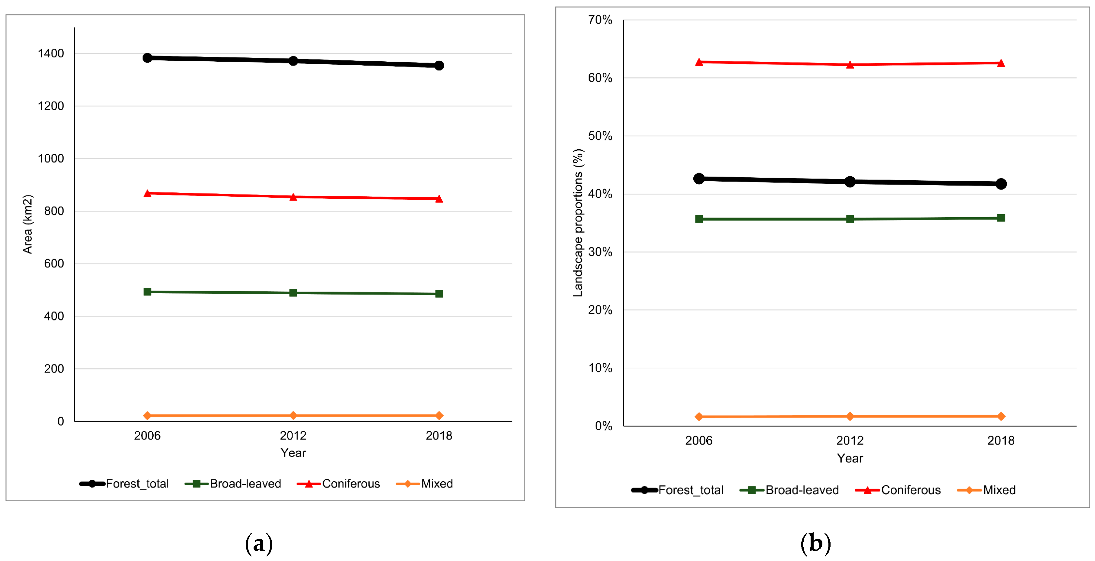
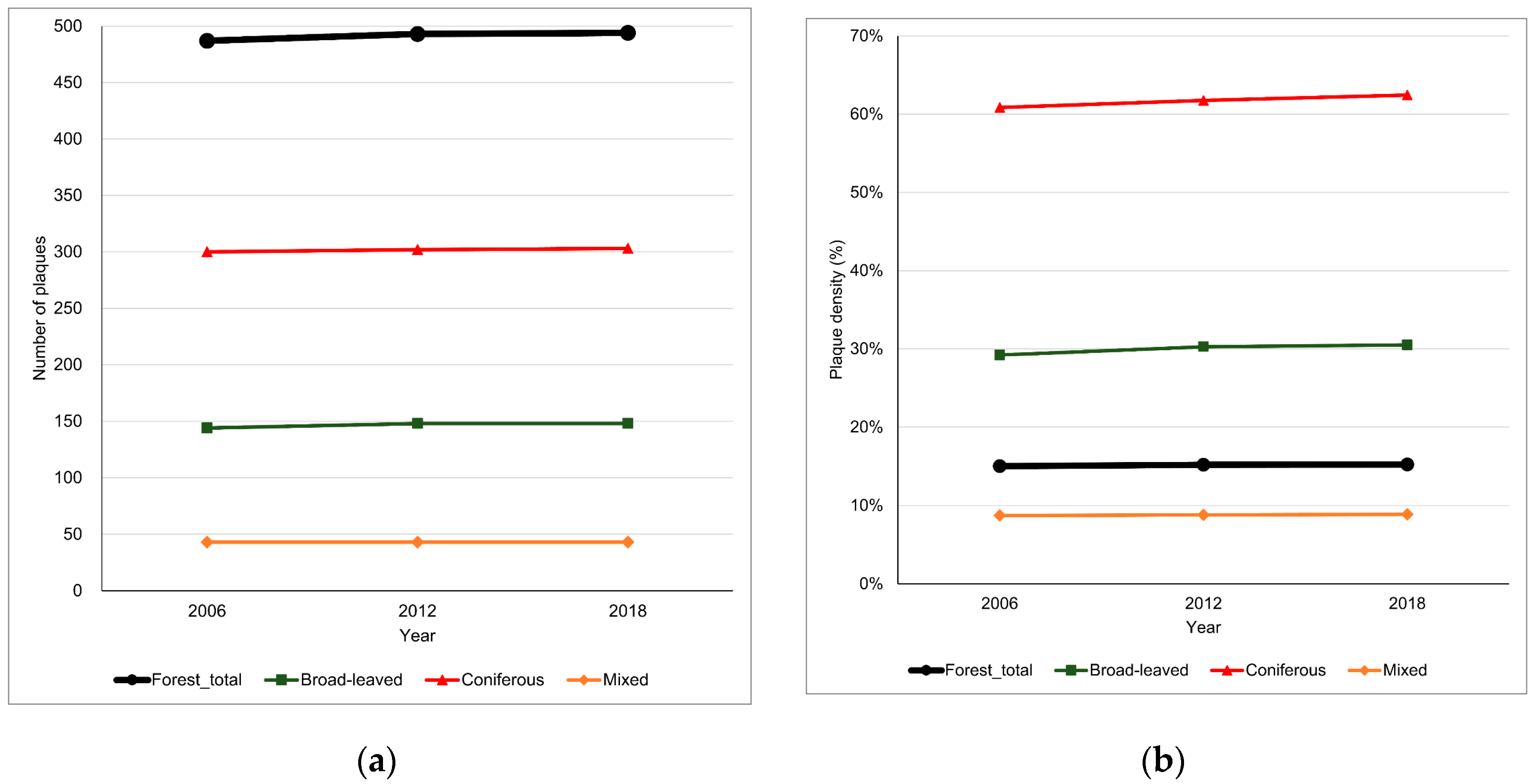
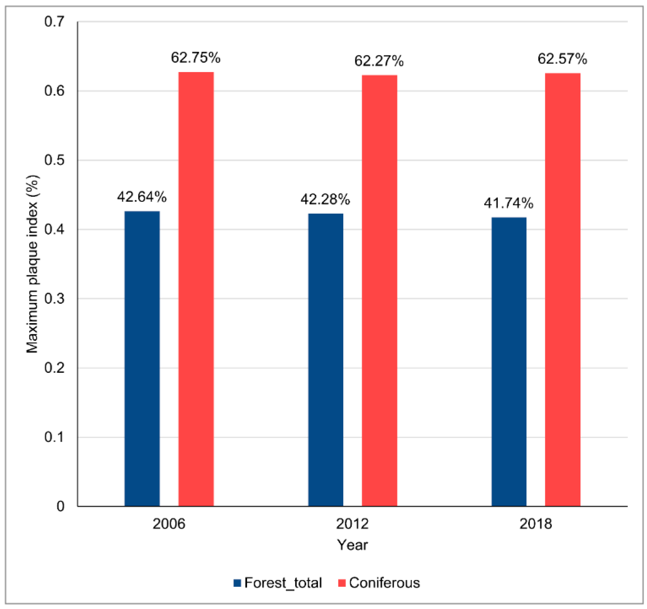
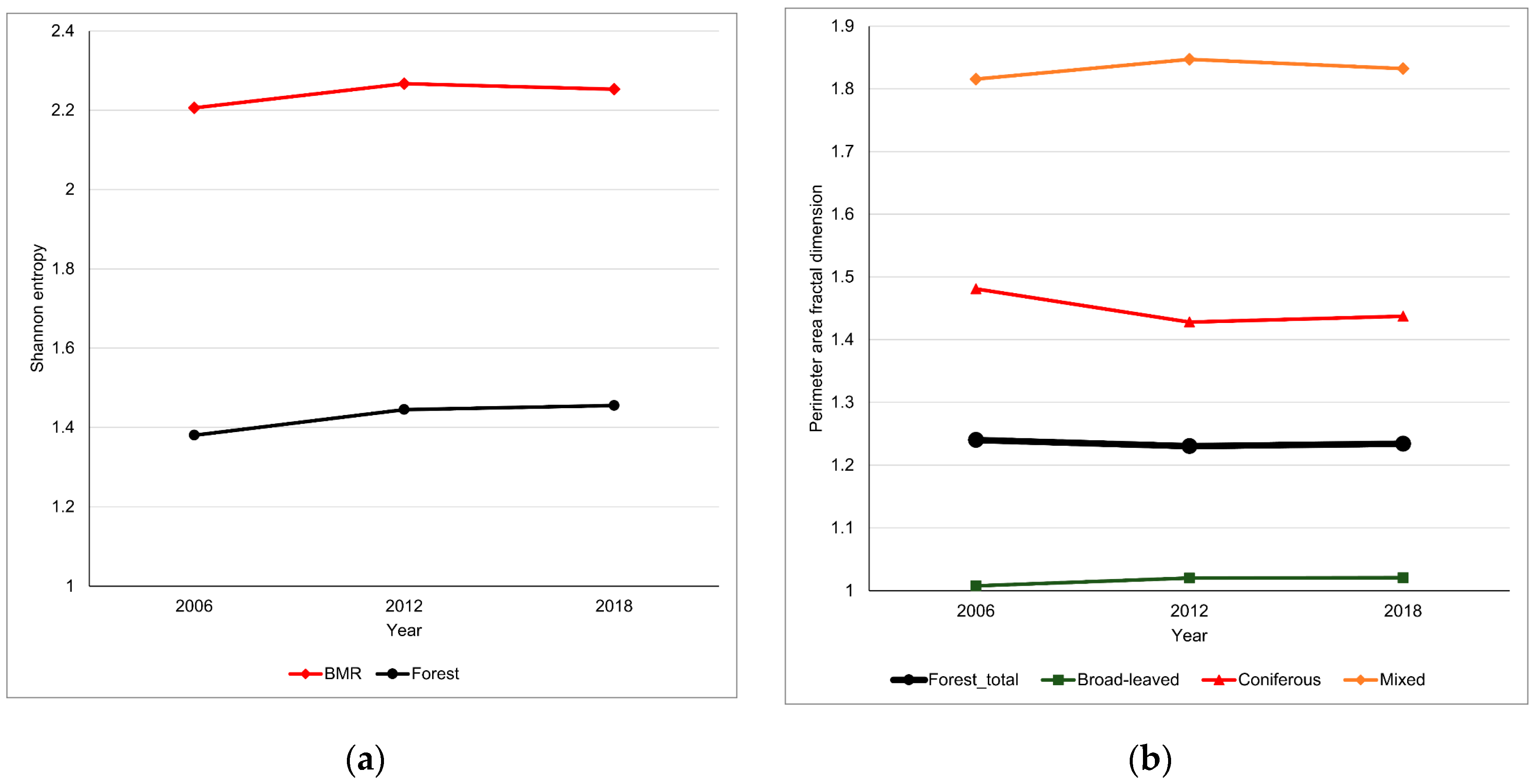
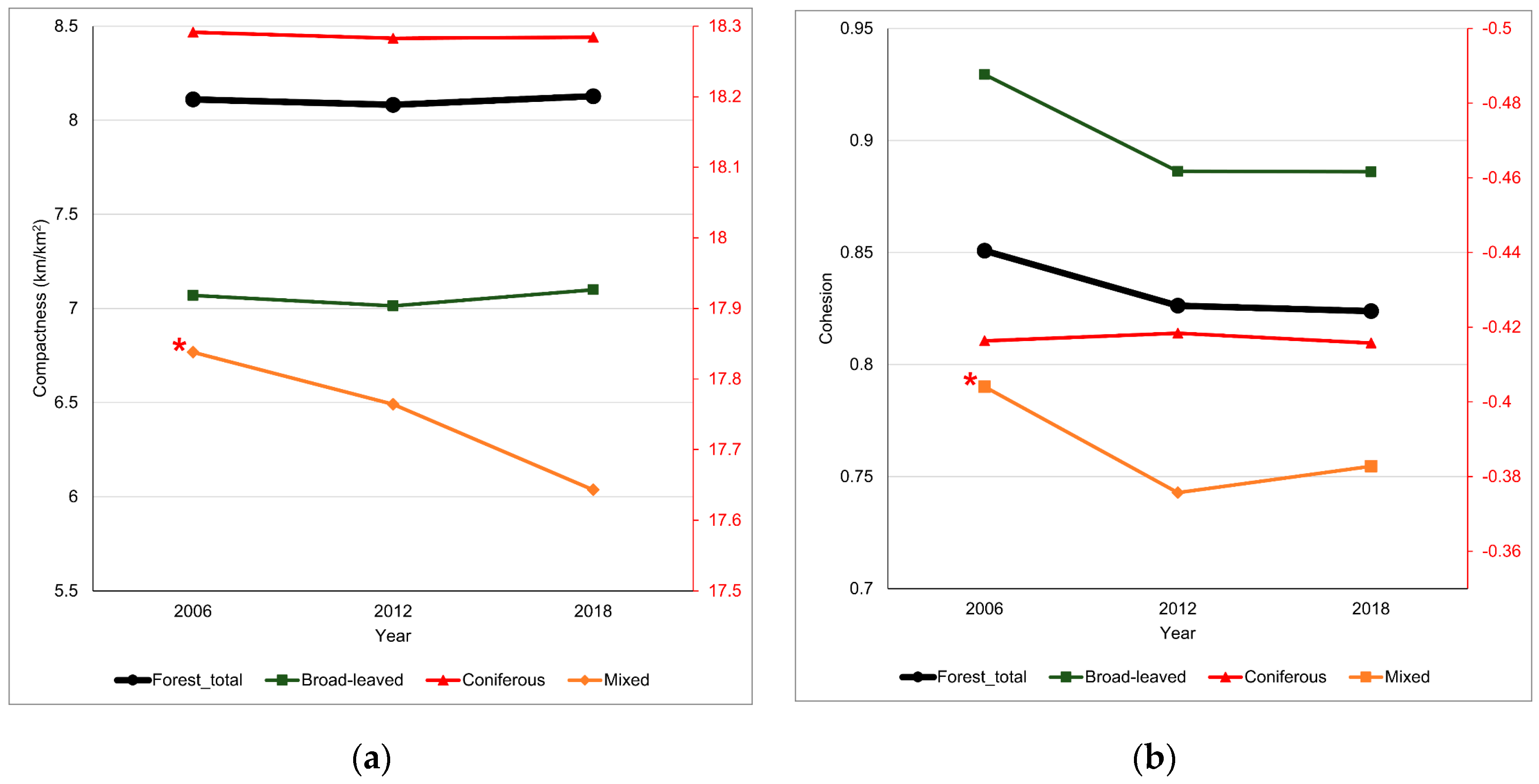
- First of all, we need to determine the evolution of BMR forest land distribution proportions. In addition to presenting the area change process of the overall forest land and the internal classification of the forest, we will analyze it from the following seven indicators.
- 2.
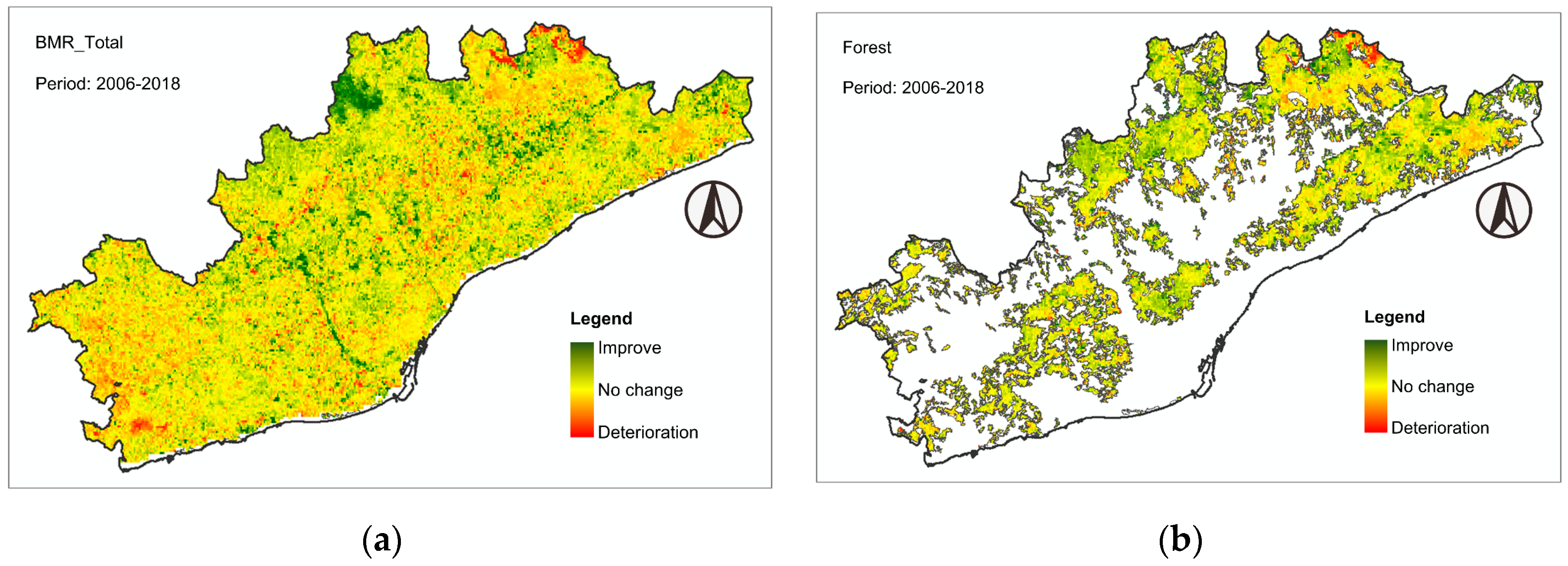
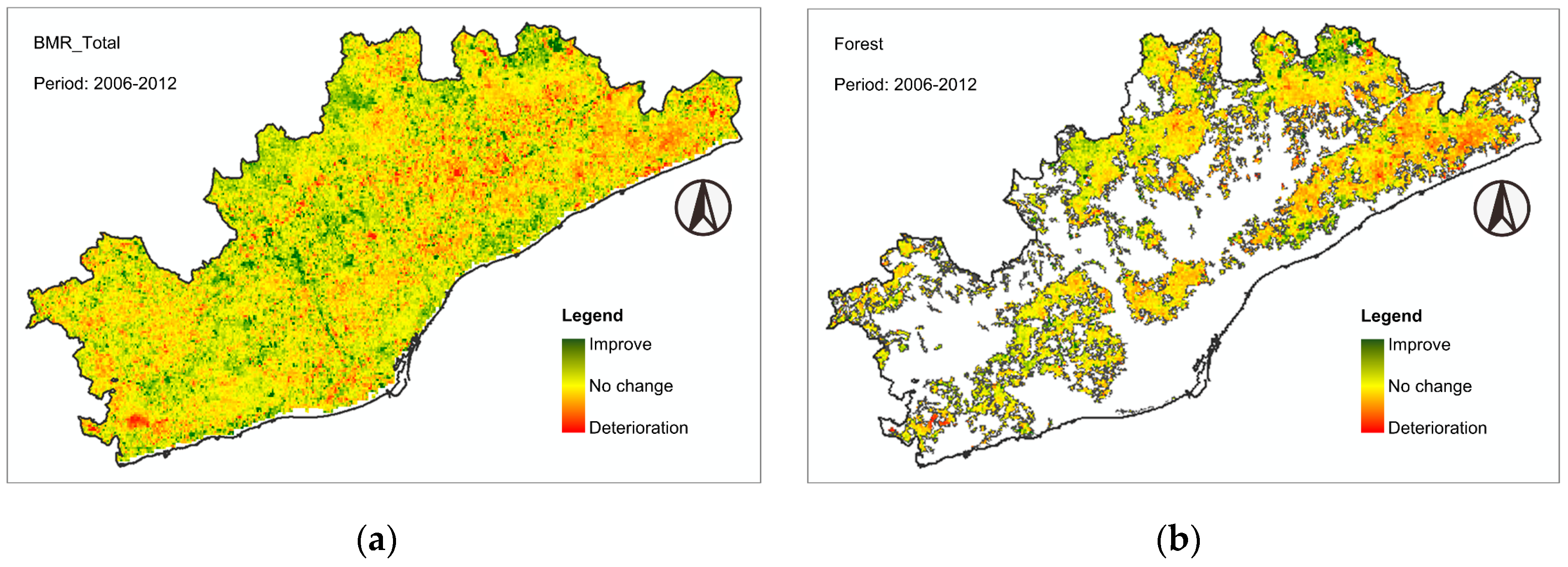
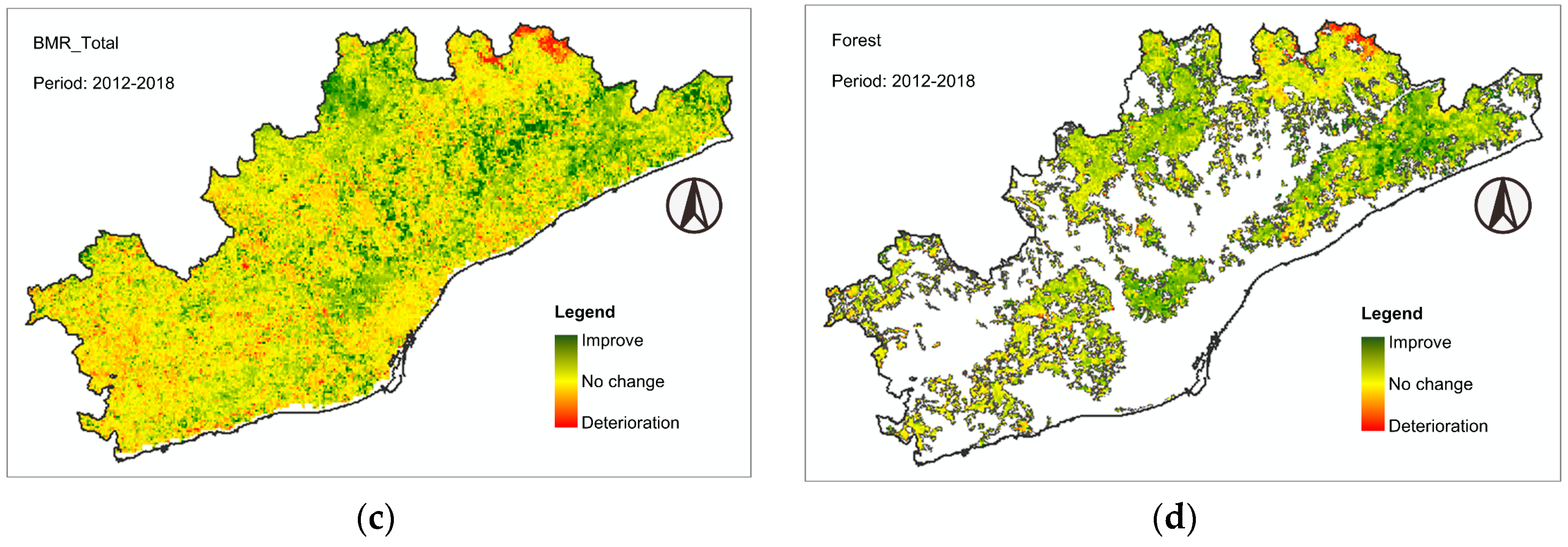
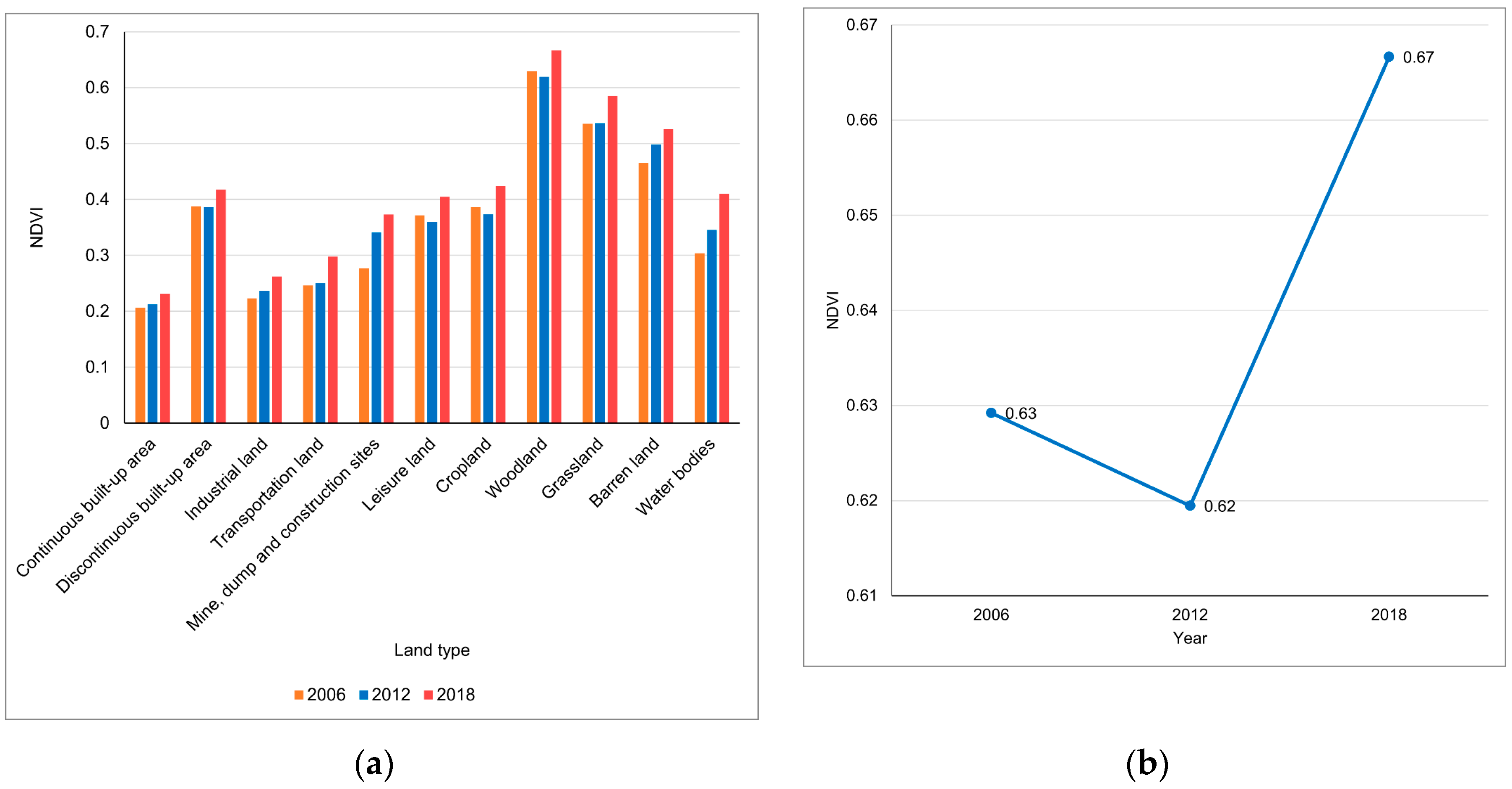
- Secondly, in order to intuitively and accurately reveal the long-term change characteristics of forest NDVI, the change of each pixel is calculated to reflect the increase or degradation trends of NDVI over time.
- 3.
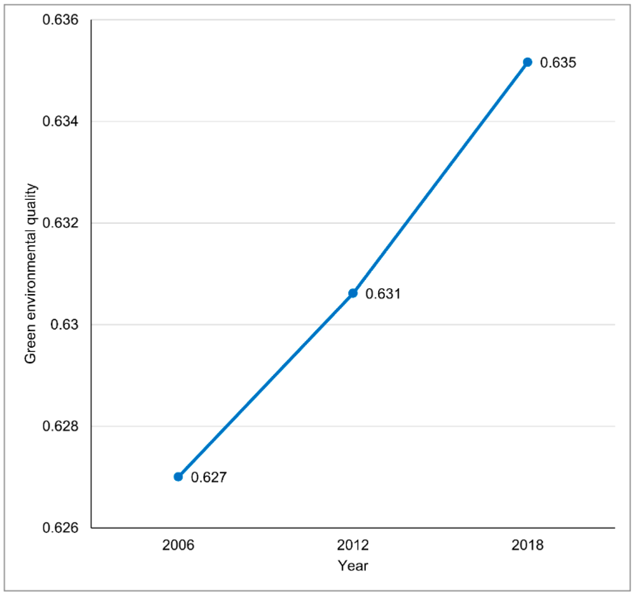
- Next, we will try to use NDVI to evaluate the forest green environmental quality of BMR. The average NDVI of each type of forest land was extracted to establish a normalized green quality assessment system. The average NDVI of each type of forest land is extracted, and for each year, we establish a normalized green quality assessment system through formula (8). Set the minimum value to 0 and the maximum value to 1 as the assigned value (Ei) of the green environmental quality proportion of each type of forest species.
- 4.
- We need to study the relationship between forest area distribution and various possible influencing factors. We will establish a 1km grid within the metropolitan area and extract the annual proportion of forest area within the grid and the average value of winter and summer NDVI. In addition, collect various types of data listed in the table. MODIS can provide land surface temperature (LST) and normalized building index NDBI. The urban heat island (UHI) effect will be represented by the urban-rural temperature difference, that is, the difference in average surface temperature between built-up areas and rural areas is expressed based on land cover data. For each year's daytime and nighttime LST, we subtract their average values in the rural land to get the approximate intensity distribution of UHI. The larger the value, the higher the UHI intensity. DEM terrain data comes from SRTM with a resolution of 30m. The impervious ground data comes from GlobeLand 30, also with a resolution of 30 meters. E-OBS can provide annual and monthly European precipitation raster data, but the resolution is 1° and the scale is very large. Therefore, we used the Kriging interpolation method to re-establish the BMR precipitation map with a resolution of 1 kilometer based on the E-OBS precipitation data. After obtaining the above data, we used the proportion of forest area in each grid as the dependent variable to establish an OLS model to analyze their importance.Table 1. List of factors potentially influencing forest spatial distribution.
Type Factors Natural factors Loçngitude Latitude Distance from coastline Orientation Altitude NDVI Precipitation LST Human activity NDBI Urban heat island effect Impermeable area Artificial area
- 5.
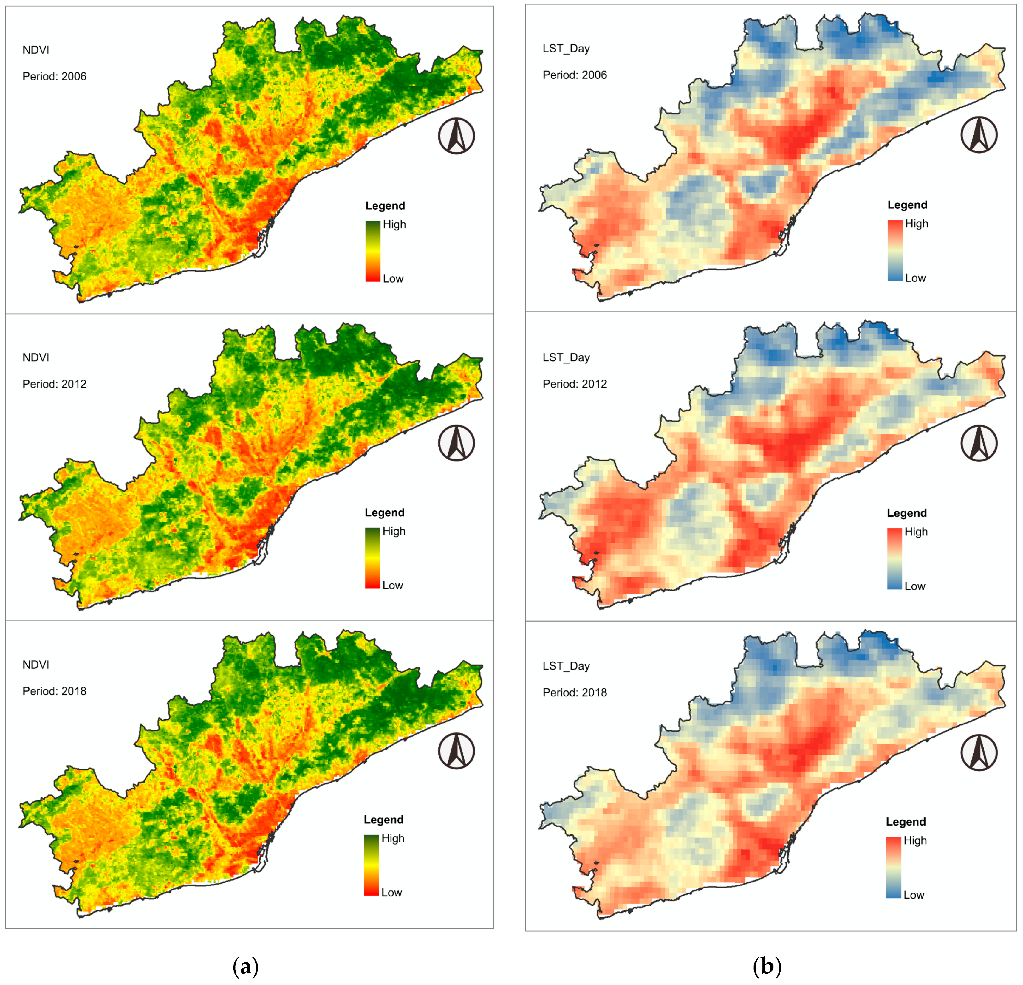
- Once it is clear that there is an obvious interaction between NDVI and forests, we must analyze the climate factors that affect NDVI to discover the potential threats that climate change may have on forests and predict possible trends in changes in BMR forest layout caused by climate change. Based on the data obtained from the grid in step 4, we used average NDVI as the dependent variable, annual precipitation and daytime and nighttime LST as independent variables to establish three OLS regression models to analyze the correlation between them and the average NDVI. And analyze the average NDVI and the distribution pattern of the found most significant independent variables on the map.
- 6.
- It is also very important to study the impact of various factors on forest landscape indicators. Taking 2018 as an example, we calculated the landscape indicators in each grid and used them as independent variables to establish models with the factors involved in the fourth step to analyze their relationships. In order to build models, it is necessary to cut the BMR into 1km grids and the landscape index inside each grid is calculated separately. Because of that, the results calculated by PAFRAC, COHESION and some other indices seriously deviate from the actual situation, and such analysis is meaningless. In addition, the landscape proportion (PLAND) index has been analyzed as a dependent variable in step 4. Therefore, in this section we only analyze patch density (PD), compactness and Shannon entropy (ENT). In addition, we will also consider the impact of temperature changes from 2006 to 2018 on forest pattern morphology.
- 7.
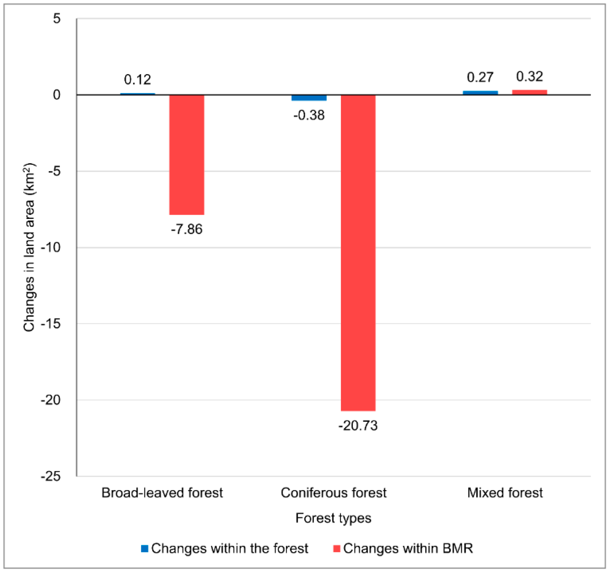
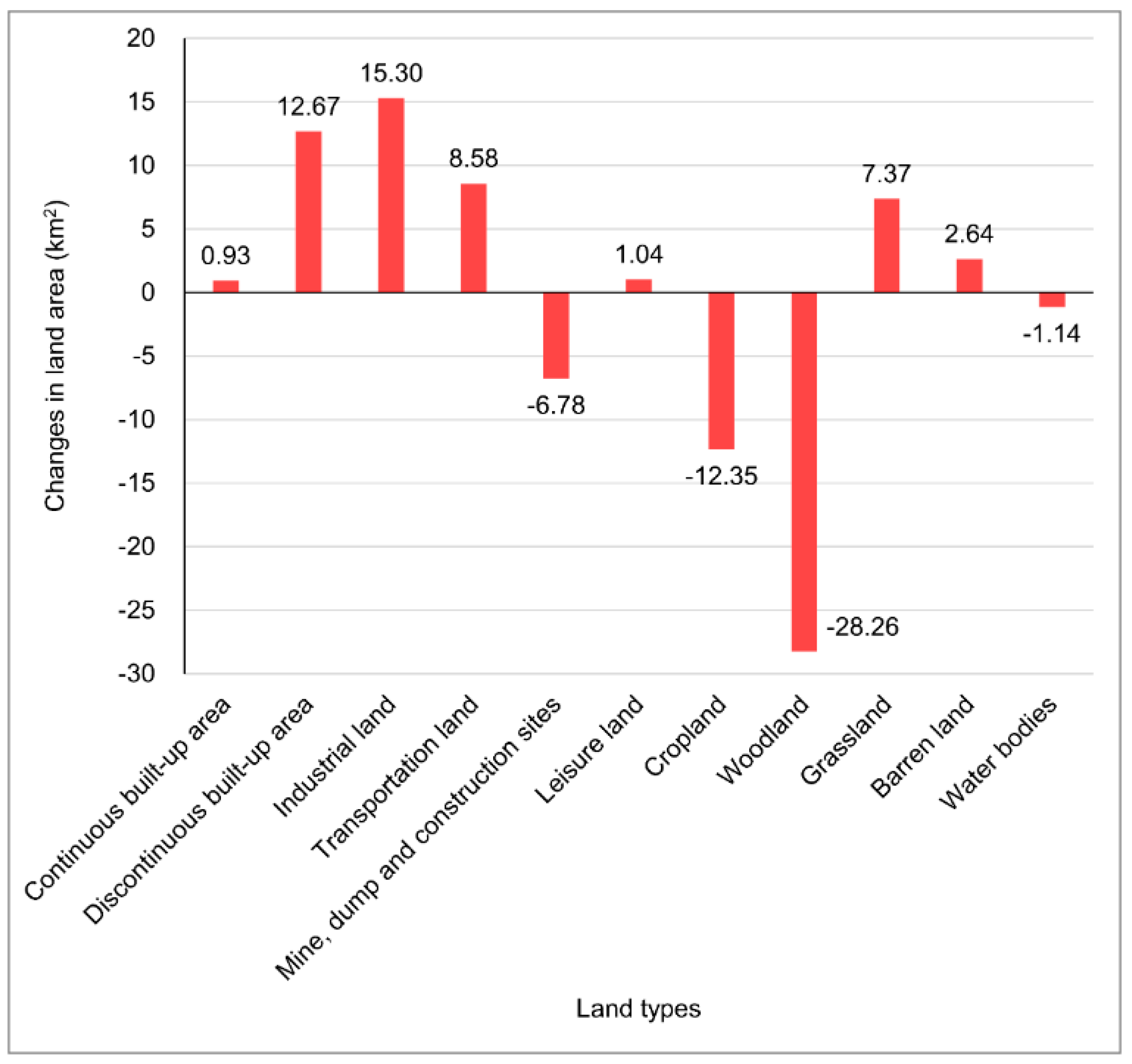
- Finally, ArcGIS was used to analyze the transformation process within the forest areas of the Barcelona metropolitan area between 2006 and 2018, and find the types of forest land that were being lost and the types that were growing significantly over the years. In addition, land transfer in the entire metropolitan area also needs to be analyzed to find the main degradation directions of forest areas.
3. Results
3.1. Analysis of Forest-Related Landscape Indicators
3.1.1. The Overall Scale of the Forest Landscape Has Been Slightly Reduced
3.1.2. Increased Fragmentation of Forest Landscapes
3.1.3. Forests Are the Most Widespread Type of Land Use
3.1.4. The Structure of Forest Land Is Becoming More Complex and the Degree of Human Interference Is Deepening
3.1.5. Forest Land Is Increasingly Dispersed
3.2. NDVI Change Trend Analysis
3.2.1. The Development of NDVI in BMR and Forest Areas Is Relatively Optimistic
3.2.2. The Development Status of NDVI in 2012 Was Disappointing
3.2.3. The Forest's NDVI Is the Most Outstanding
3.3. Forest Green Environmental Quality Assessment
3.3.1. Broadleaf Forest Has the Highest Assessment Weight
3.3.2. The Quality of Forest Green Environment Is Increasing Year by Year
3.4. Analysis of Factors Affecting Forest Distribution
3.5. Analysis of Climate Factors Affecting NDVI
3.6. Analysis of Influencing Factors of Forest Landscape Index
| Independent variable d | Model_PD a | Model_ENT b | Model_Compactness c | |||||||||||
|---|---|---|---|---|---|---|---|---|---|---|---|---|---|---|
| B | Beta | t | Sig. | B | Beta | t | Sig. | B | Beta | t | Sig. | |||
| Constant | -4549.12 | - | -3.66 | 0.00 | -0.08 | - | -3.34 | 0.00 | -372.52 | - | -0.12 | 0.905 | ||
| Longitude | 0.00 | -0.44 | -3.71 | 0.00 | 0.00 | -0.41 | -3.38 | 0.00 | 0.00 | 0.02 | 0.07 | 0.943 | ||
| Latitude | 0.00 | 0.47 | 3.66 | 0.00 | 0.00 | 0.43 | 3.31 | 0.00 | 0.00 | 0.07 | 0.30 | 0.768 | ||
| Distance from coastline | 0.00 | -0.20 | -2.54 | 0.01 | 0.00 | -0.18 | -2.28 | 0.02 | 0.00 | -0.09 | -0.68 | 0.498 | ||
| Orientation | 0.00 | 0.00 | -0.28 | 0.78 | 0.00 | -0.01 | -0.36 | 0.72 | -0.01 | 0.00 | -0.17 | 0.862 | ||
| Altitude | -0.02 | -0.10 | -3.42 | 0.00 | 0.00 | -0.10 | -3.29 | 0.00 | 0.01 | 0.03 | 0.53 | 0.599 | ||
| Slope | 1.18 | 0.01 | 0.82 | 0.41 | 0.00 | 0.02 | 1.05 | 0.29 | -6.09 | -0.04 | -1.68 | 0.093 | ||
| NDVI_MEAN | 91.58 | 0.34 | 8.20 | 0.00 | 0.00 | 0.36 | 8.47 | 0.00 | -83.81 | -0.22 | -2.98 | 0.003 | ||
| Precipitation | 1.62 | 0.05 | 2.38 | 0.02 | 0.00 | 0.05 | 2.31 | 0.02 | -0.87 | -0.02 | -0.51 | 0.611 | ||
| LST_DAY | -3.63 | -0.22 | -7.38 | 0.00 | 0.00 | -0.22 | -7.23 | 0.00 | 2.85 | 0.12 | 2.31 | 0.021 | ||
| LST_NIGHT | 3.38 | 0.11 | 4.06 | 0.00 | 0.00 | 0.11 | 3.85 | 0.00 | -2.59 | -0.06 | -1.24 | 0.216 | ||
| NDBI | -70.13 | -0.33 | -7.87 | 0.00 | 0.00 | -0.32 | -7.44 | 0.00 | 3.73 | 0.01 | 0.17 | 0.868 | ||
| Impermeable area | 4.19 | 0.03 | 0.58 | 0.56 | 0.00 | 0.04 | 0.86 | 0.39 | 14.88 | 0.06 | 0.82 | 0.411 | ||
| Artificial area | -20.75 | -0.13 | -2.98 | 0.00 | 0.00 | -0.14 | -3.12 | 0.00 | -0.86 | 0.00 | -0.05 | 0.961 | ||
| Difference_LST_DAY_2018-2006 | 4.78 | 0.13 | 6.70 | 0.00 | 0.00 | 0.13 | 6.47 | 0.00 | -3.82 | -0.07 | -2.12 | 0.034 | ||
| Difference_LST_NIGHT_2018-2006 | -2.23 | -0.05 | -2.15 | 0.03 | 0.00 | -0.04 | -2.00 | 0.05 | 5.47 | 0.08 | 2.10 | 0.036 | ||
3.7. Land Use Transfer Matrix Analysis
3.7.1. Mixed Forests Are the Only Expanding Woodlands
3.7.2. Forests Are Mainly Transferred Like Cultivated Land and Grassland
4. Discussion and Conclusion
Author Contributions
Funding
Institutional Review Board Statement
Informed Consent Statement
Data Availability Statement
Acknowledgments
Conflicts of Interest
Appendix A
| Classification results | CLC land use description |
| Continuous built-up area | Continuous urban fabric |
| Discontinuous built-up area | Discontinuous urban fabric |
| Industrial land | Industrial or commercial units |
| Transportation land | Road and rail networks and associated land |
| Port areas | |
| Airports | |
| Mine, dump and construction sites | Mineral extraction sites |
| Dump sites | |
| Construction sites | |
| Leisure land | Green urban areas |
| Sport and leisure facilities | |
| Cropland | Non-irrigated arable land |
| Permanently irrigated land | |
| Rice fields | |
| Vineyards | |
| Fruit trees and berry plantations | |
| Olive groves | |
| Pastures | |
| Annual crops associated with permanent crops | |
| Complex cultivation patterns | |
| Land principally occupied by agriculture, with significant areas of natural vegetation | |
| Agro-forestry areas | |
| Woodland | Broad-leaved forest |
| Coniferous forest | |
| Mixed forest | |
| Grassland | Natural grasslands |
| Moors and heathland | |
| Sclerophyllous vegetation | |
| Transitional woodland-shrub | |
| Inland marshes | |
| Peat bogs | |
| Salt marshes | |
| Barren land | Beaches, dunes, sands |
| Bare rocks | |
| Sparsely vegetated areas | |
| Burnt areas | |
| Glaciers and perpetual snow | |
| Salines | |
| Intertidal flats | |
| Water bodies | Water courses |
| Water bodies | |
| Coastal lagoons | |
| Estuaries | |
| Sea and ocean |
Appendix B
| Var. | 1 | 2 | 3 | 4 | 5 | 6 | 7 | 8 | 9 | 10 | 11 | 12 | 13 | 14 | 15 | 16 | |
| 1 | Pearson | 1 | .331** | .341** | 0.03 | .100** | .387** | .230** | .824** | .410** | -.690** | -.102** | -.796** | -.690** | -.102** | -.447** | -.480** |
| Sign. | 0 | 0 | 0.146 | 0 | 0 | 0 | 0 | 0 | 0 | 0 | 0 | 0 | 0 | 0 | 0 | ||
| N. cases | 2283 | 2283 | 2283 | 2283 | 2283 | 2283 | 2283 | 2273 | 2283 | 1740 | 1740 | 2280 | 1740 | 1740 | 2283 | 2283 | |
| 2 | Pearson | .331** | 1 | .724** | -.320** | 0.032 | -0.002 | 0.03 | .387** | .893** | -.287** | .325** | -.439** | -.287** | .325** | 0.021 | 0.01 |
| Sign. | 0 | 0 | 0 | 0.131 | 0.914 | 0.153 | 0 | 0 | 0 | 0 | 0 | 0 | 0 | 0.314 | 0.629 | ||
| N. cases | 2283 | 2283 | 2283 | 2283 | 2283 | 2283 | 2283 | 2273 | 2283 | 1740 | 1740 | 2280 | 1740 | 1740 | 2283 | 2283 | |
| 3 | Pearson | .341** | .724** | 1 | .404** | 0.028 | .448** | .078** | .352** | .863** | -.388** | -.221** | -.388** | -.388** | -.221** | -.093** | -.116** |
| Sign. | 0 | 0 | 0 | 0.186 | 0 | 0 | 0 | 0 | 0 | 0 | 0 | 0 | 0 | 0 | 0 | ||
| N. cases | 2283 | 2283 | 2283 | 2283 | 2283 | 2283 | 2283 | 2273 | 2283 | 1740 | 1740 | 2280 | 1740 | 1740 | 2283 | 2283 | |
| 4 | Pearson | 0.03 | -.320** | .404** | 1 | -0.005 | .578** | .085** | -0.037 | -0.022 | -.176** | -.692** | 0.038 | -.176** | -.692** | -.126** | -.140** |
| Sign. | 0.146 | 0 | 0 | 0.799 | 0 | 0 | 0.076 | 0.285 | 0 | 0 | 0.069 | 0 | 0 | 0 | 0 | ||
| N. cases | 2283 | 2283 | 2283 | 2283 | 2283 | 2283 | 2283 | 2273 | 2283 | 1740 | 1740 | 2280 | 1740 | 1740 | 2283 | 2283 | |
| 5 | Pearson | .100** | 0.032 | 0.028 | -0.005 | 1 | .103** | .058** | .116** | .067** | -.077** | -.097** | -.097** | -.077** | -.097** | -.077** | -.080** |
| Sign. | 0 | 0.131 | 0.186 | 0.799 | 0 | 0.006 | 0 | 0.001 | 0.001 | 0 | 0 | 0.001 | 0 | 0 | 0 | ||
| N. cases | 2283 | 2283 | 2283 | 2283 | 2283 | 2283 | 2283 | 2273 | 2283 | 1740 | 1740 | 2280 | 1740 | 1740 | 2283 | 2283 | |
| 6 | Pearson | .387** | -0.002 | .448** | .578** | .103** | 1 | .192** | .454** | .332** | -.612** | -.724** | -.444** | -.612** | -.724** | -.336** | -.356** |
| Sign. | 0 | 0.914 | 0 | 0 | 0 | 0 | 0 | 0 | 0 | 0 | 0 | 0 | 0 | 0 | 0 | ||
| N. cases | 2283 | 2283 | 2283 | 2283 | 2283 | 2283 | 2283 | 2273 | 2283 | 1740 | 1740 | 2280 | 1740 | 1740 | 2283 | 2283 | |
| 7 | Pearson | .230** | 0.03 | .078** | .085** | .058** | .192** | 1 | .254** | .060** | -.231** | -.055* | -.203** | -.231** | -.055* | -.139** | -.153** |
| Sign. | 0 | 0.153 | 0 | 0 | 0.006 | 0 | 0 | 0.004 | 0 | 0.022 | 0 | 0 | 0.022 | 0 | 0 | ||
| N. cases | 2283 | 2283 | 2283 | 2283 | 2283 | 2283 | 2283 | 2273 | 2283 | 1740 | 1740 | 2280 | 1740 | 1740 | 2283 | 2283 | |
| 8 | Pearson | .824** | .387** | .352** | -0.037 | .116** | .454** | .254** | 1 | .469** | -.732** | -.111** | -.911** | -.732** | -.111** | -.524** | -.565** |
| Sign. | 0 | 0 | 0 | 0.076 | 0 | 0 | 0 | 0 | 0 | 0 | 0 | 0 | 0 | 0 | 0 | ||
| N. cases | 2273 | 2273 | 2273 | 2273 | 2273 | 2273 | 2273 | 2273 | 2273 | 1732 | 1732 | 2273 | 1732 | 1732 | 2273 | 2273 | |
| 9 | Pearson | .410** | .893** | .863** | -0.022 | .067** | .332** | .060** | .469** | 1 | -.413** | -0.008 | -.512** | -.413** | -0.008 | -.090** | -.107** |
| Sign. | 0 | 0 | 0 | 0.285 | 0.001 | 0 | 0.004 | 0 | 0 | 0.733 | 0 | 0 | 0.733 | 0 | 0 | ||
| N. cases | 2283 | 2283 | 2283 | 2283 | 2283 | 2283 | 2283 | 2273 | 2283 | 1740 | 1740 | 2280 | 1740 | 1740 | 2283 | 2283 | |
| 10 | Pearson | -.690** | -.287** | -.388** | -.176** | -.077** | -.612** | -.231** | -.732** | -.413** | 1 | .332** | .758** | 1.000** | .332** | .297** | .334** |
| Sign. | 0 | 0 | 0 | 0 | 0.001 | 0 | 0 | 0 | 0 | 0 | 0 | 0 | 0 | 0 | 0 | ||
| N. cases | 1740 | 1740 | 1740 | 1740 | 1740 | 1740 | 1740 | 1732 | 1740 | 1740 | 1740 | 1738 | 1740 | 1740 | 1740 | 1740 | |
| 11 | Pearson | -.102** | .325** | -.221** | -.692** | -.097** | -.724** | -.055* | -.111** | -0.008 | .332** | 1 | .082** | .332** | 1.000** | .320** | .345** |
| Sign. | 0 | 0 | 0 | 0 | 0 | 0 | 0.022 | 0 | 0.733 | 0 | 0.001 | 0 | 0 | 0 | 0 | ||
| N. cases | 1740 | 1740 | 1740 | 1740 | 1740 | 1740 | 1740 | 1732 | 1740 | 1740 | 1740 | 1738 | 1740 | 1740 | 1740 | 1740 | |
| 12 | Pearson | -.796** | -.439** | -.388** | 0.038 | -.097** | -.444** | -.203** | -.911** | -.512** | .758** | .082** | 1 | .758** | .082** | .388** | .425** |
| Sign. | 0 | 0 | 0 | 0.069 | 0 | 0 | 0 | 0 | 0 | 0 | 0.001 | 0 | 0.001 | 0 | 0 | ||
| N. cases | 2280 | 2280 | 2280 | 2280 | 2280 | 2280 | 2280 | 2273 | 2280 | 1738 | 1738 | 2280 | 1738 | 1738 | 2280 | 2280 | |
| 13 | Pearson | -.690** | -.287** | -.388** | -.176** | -.077** | -.612** | -.231** | -.732** | -.413** | 1.000** | .332** | .758** | 1 | .332** | .297** | .334** |
| Sign. | 0 | 0 | 0 | 0 | 0.001 | 0 | 0 | 0 | 0 | 0 | 0 | 0 | 0 | 0 | 0 | ||
| N. cases | 1740 | 1740 | 1740 | 1740 | 1740 | 1740 | 1740 | 1732 | 1740 | 1740 | 1740 | 1738 | 1740 | 1740 | 1740 | 1740 | |
| 14 | Pearson | -.102** | .325** | -.221** | -.692** | -.097** | -.724** | -.055* | -.111** | -0.008 | .332** | 1.000** | .082** | .332** | 1 | .320** | .345** |
| Sign. | 0 | 0 | 0 | 0 | 0 | 0 | 0.022 | 0 | 0.733 | 0 | 0 | 0.001 | 0 | 0 | 0 | ||
| N. cases | 1740 | 1740 | 1740 | 1740 | 1740 | 1740 | 1740 | 1732 | 1740 | 1740 | 1740 | 1738 | 1740 | 1740 | 1740 | 1740 | |
| 15 | Pearson | -.447** | 0.021 | -.093** | -.126** | -.077** | -.336** | -.139** | -.524** | -.090** | .297** | .320** | .388** | .297** | .320** | 1 | .949** |
| Sign. | 0 | 0.314 | 0 | 0 | 0 | 0 | 0 | 0 | 0 | 0 | 0 | 0 | 0 | 0 | 0 | ||
| N. cases | 2283 | 2283 | 2283 | 2283 | 2283 | 2283 | 2283 | 2273 | 2283 | 1740 | 1740 | 2280 | 1740 | 1740 | 2283 | 2283 | |
| 16 | Pearson | -.480** | 0.01 | -.116** | -.140** | -.080** | -.356** | -.153** | -.565** | -.107** | .334** | .345** | .425** | .334** | .345** | .949** | 1 |
| Sign. | 0 | 0.629 | 0 | 0 | 0 | 0 | 0 | 0 | 0 | 0 | 0 | 0 | 0 | 0 | 0 | ||
| N. cases | 2283 | 2283 | 2283 | 2283 | 2283 | 2283 | 2283 | 2273 | 2283 | 1740 | 1740 | 2280 | 1740 | 1740 | 2283 | 2283 |
| Var. | 1 | 2 | 3 | 4 | 5 | 6 | 7 | 8 | 9 | 10 | 11 | 12 | 13 | 14 | 15 | 16 | |
| 1 | Pearson | 1 | .327** | .341** | 0.038 | .097** | .391** | .229** | .828** | -.322** | -.631** | -.211** | -.784** | -.631** | -.211** | -.499** | -.520** |
| Sign. | 0 | 0 | 0.073 | 0 | 0 | 0 | 0 | 0 | 0 | 0 | 0 | 0 | 0 | 0 | 0 | ||
| N. cases | 2268 | 2268 | 2268 | 2268 | 2268 | 2268 | 2268 | 2263 | 2268 | 1730 | 1730 | 2264 | 1730 | 1730 | 1178 | 1252 | |
| 2 | Pearson | .327** | 1 | .724** | -.319** | 0.031 | -0.005 | 0.028 | .343** | -.708** | -.208** | 0.014 | -.405** | -.208** | 0.014 | -0.018 | -0.009 |
| Sign. | 0 | 0 | 0 | 0.138 | 0.806 | 0.184 | 0 | 0 | 0 | 0.547 | 0 | 0 | 0.547 | 0.542 | 0.745 | ||
| N. cases | 2268 | 2268 | 2268 | 2268 | 2268 | 2268 | 2268 | 2263 | 2268 | 1730 | 1730 | 2264 | 1730 | 1730 | 1178 | 1252 | |
| 3 | Pearson | .341** | .724** | 1 | .405** | 0.027 | .447** | .077** | .349** | -.606** | -.395** | -.536** | -.446** | -.395** | -.536** | -0.056 | -.057* |
| Sign. | 0 | 0 | 0 | 0.192 | 0 | 0 | 0 | 0 | 0 | 0 | 0 | 0 | 0 | 0.053 | 0.045 | ||
| N. cases | 2268 | 2268 | 2268 | 2268 | 2268 | 2268 | 2268 | 2263 | 2268 | 1730 | 1730 | 2264 | 1730 | 1730 | 1178 | 1252 | |
| 4 | Pearson | 0.038 | -.319** | .405** | 1 | -0.005 | .582** | .086** | 0.027 | .156** | -.278** | -.729** | -.097** | -.278** | -.729** | -0.031 | -0.04 |
| Sign. | 0.073 | 0 | 0 | 0.826 | 0 | 0 | 0.195 | 0 | 0 | 0 | 0 | 0 | 0 | 0.287 | 0.16 | ||
| N. cases | 2268 | 2268 | 2268 | 2268 | 2268 | 2268 | 2268 | 2263 | 2268 | 1730 | 1730 | 2264 | 1730 | 1730 | 1178 | 1252 | |
| 5 | Pearson | .097** | 0.031 | 0.027 | -0.005 | 1 | .101** | .058** | .111** | -0.002 | -.069** | -.127** | -.105** | -.069** | -.127** | -0.048 | -.061* |
| Sign. | 0 | 0.138 | 0.192 | 0.826 | 0 | 0.006 | 0 | 0.932 | 0.004 | 0 | 0 | 0.004 | 0 | 0.102 | 0.032 | ||
| N. cases | 2268 | 2268 | 2268 | 2268 | 2268 | 2268 | 2268 | 2263 | 2268 | 1730 | 1730 | 2264 | 1730 | 1730 | 1178 | 1252 | |
| 6 | Pearson | .391** | -0.005 | .447** | .582** | .101** | 1 | .191** | .508** | -.138** | -.731** | -.830** | -.558** | -.731** | -.830** | -.228** | -.256** |
| Sign. | 0 | 0.806 | 0 | 0 | 0 | 0 | 0 | 0 | 0 | 0 | 0 | 0 | 0 | 0 | 0 | ||
| N. cases | 2268 | 2268 | 2268 | 2268 | 2268 | 2268 | 2268 | 2263 | 2268 | 1730 | 1730 | 2264 | 1730 | 1730 | 1178 | 1252 | |
| 7 | Pearson | .229** | 0.028 | .077** | .086** | .058** | .191** | 1 | .276** | -0.01 | -.229** | -.087** | -.219** | -.229** | -.087** | -.203** | -.238** |
| Sign. | 0 | 0.184 | 0 | 0 | 0.006 | 0 | 0 | 0.635 | 0 | 0 | 0 | 0 | 0 | 0 | 0 | ||
| N. cases | 2268 | 2268 | 2268 | 2268 | 2268 | 2268 | 2268 | 2263 | 2268 | 1730 | 1730 | 2264 | 1730 | 1730 | 1178 | 1252 | |
| 8 | Pearson | .828** | .343** | .349** | 0.027 | .111** | .508** | .276** | 1 | -.340** | -.727** | -.276** | -.907** | -.727** | -.276** | -.527** | -.566** |
| Sign. | 0 | 0 | 0 | 0.195 | 0 | 0 | 0 | 0 | 0 | 0 | 0 | 0 | 0 | 0 | 0 | ||
| N. cases | 2263 | 2263 | 2263 | 2263 | 2263 | 2263 | 2263 | 2263 | 2263 | 1726 | 1726 | 2263 | 1726 | 1726 | 1173 | 1247 | |
| 9 | Pearson | -.322** | -.708** | -.606** | .156** | -0.002 | -.138** | -0.01 | -.340** | 1 | .311** | .149** | .329** | .311** | .149** | .143** | .148** |
| Sign. | 0 | 0 | 0 | 0 | 0.932 | 0 | 0.635 | 0 | 0 | 0 | 0 | 0 | 0 | 0 | 0 | ||
| N. cases | 2268 | 2268 | 2268 | 2268 | 2268 | 2268 | 2268 | 2263 | 2268 | 1730 | 1730 | 2264 | 1730 | 1730 | 1178 | 1252 | |
| 10 | Pearson | -.631** | -.208** | -.395** | -.278** | -.069** | -.731** | -.229** | -.727** | .311** | 1 | .573** | .764** | 1.000** | .573** | .213** | .244** |
| Sign. | 0 | 0 | 0 | 0 | 0.004 | 0 | 0 | 0 | 0 | 0 | 0 | 0 | 0 | 0 | 0 | ||
| N. cases | 1730 | 1730 | 1730 | 1730 | 1730 | 1730 | 1730 | 1726 | 1730 | 1730 | 1730 | 1727 | 1730 | 1730 | 890 | 955 | |
| 11 | Pearson | -.211** | 0.014 | -.536** | -.729** | -.127** | -.830** | -.087** | -.276** | .149** | .573** | 1 | .349** | .573** | 1.000** | .187** | .217** |
| Sign. | 0 | 0.547 | 0 | 0 | 0 | 0 | 0 | 0 | 0 | 0 | 0 | 0 | 0 | 0 | 0 | ||
| N. cases | 1730 | 1730 | 1730 | 1730 | 1730 | 1730 | 1730 | 1726 | 1730 | 1730 | 1730 | 1727 | 1730 | 1730 | 890 | 955 | |
| 12 | Pearson | -.784** | -.405** | -.446** | -.097** | -.105** | -.558** | -.219** | -.907** | .329** | .764** | .349** | 1 | .764** | .349** | .371** | .405** |
| Sign. | 0 | 0 | 0 | 0 | 0 | 0 | 0 | 0 | 0 | 0 | 0 | 0 | 0 | 0 | 0 | ||
| N. cases | 2264 | 2264 | 2264 | 2264 | 2264 | 2264 | 2264 | 2263 | 2264 | 1727 | 1727 | 2264 | 1727 | 1727 | 1174 | 1248 | |
| 13 | Pearson | -.631** | -.208** | -.395** | -.278** | -.069** | -.731** | -.229** | -.727** | .311** | 1.000** | .573** | .764** | 1 | .573** | .213** | .244** |
| Sign. | 0 | 0 | 0 | 0 | 0.004 | 0 | 0 | 0 | 0 | 0 | 0 | 0 | 0 | 0 | 0 | ||
| N. cases | 1730 | 1730 | 1730 | 1730 | 1730 | 1730 | 1730 | 1726 | 1730 | 1730 | 1730 | 1727 | 1730 | 1730 | 890 | 955 | |
| 14 | Pearson | -.211** | 0.014 | -.536** | -.729** | -.127** | -.830** | -.087** | -.276** | .149** | .573** | 1.000** | .349** | .573** | 1 | .187** | .217** |
| Sign. | 0 | 0.547 | 0 | 0 | 0 | 0 | 0 | 0 | 0 | 0 | 0 | 0 | 0 | 0 | 0 | ||
| N. cases | 1730 | 1730 | 1730 | 1730 | 1730 | 1730 | 1730 | 1726 | 1730 | 1730 | 1730 | 1727 | 1730 | 1730 | 890 | 955 | |
| 15 | Pearson | -.499** | -0.018 | -0.056 | -0.031 | -0.048 | -.228** | -.203** | -.527** | .143** | .213** | .187** | .371** | .213** | .187** | 1 | .953** |
| Sign. | 0 | 0.542 | 0.053 | 0.287 | 0.102 | 0 | 0 | 0 | 0 | 0 | 0 | 0 | 0 | 0 | 0 | ||
| N. cases | 1178 | 1178 | 1178 | 1178 | 1178 | 1178 | 1178 | 1173 | 1178 | 890 | 890 | 1174 | 890 | 890 | 1178 | 1178 | |
| 16 | Pearson | -.520** | -0.009 | -.057* | -0.04 | -.061* | -.256** | -.238** | -.566** | .148** | .244** | .217** | .405** | .244** | .217** | .953** | 1 |
| Sign. | 0 | 0.745 | 0.045 | 0.16 | 0.032 | 0 | 0 | 0 | 0 | 0 | 0 | 0 | 0 | 0 | 0 | ||
| N. cases | 1252 | 1252 | 1252 | 1252 | 1252 | 1252 | 1252 | 1247 | 1252 | 955 | 955 | 1248 | 955 | 955 | 1178 | 1252 |
| Var. | 1 | 2 | 3 | 4 | 5 | 6 | 7 | 8 | 9 | 10 | 11 | 12 | 13 | 14 | 15 | 16 | |
| 1 | Pearson | 1 | .330** | .343** | 0.038 | .097** | .384** | .227** | .811** | .205** | -.602** | -.229** | -.801** | -.602** | -.229** | -.459** | -.490** |
| Sign. | 0 | 0 | 0.072 | 0 | 0 | 0 | 0 | 0 | 0 | 0 | 0 | 0 | 0 | 0 | 0 | ||
| N. cases | 2264 | 2264 | 2264 | 2264 | 2264 | 2264 | 2264 | 2255 | 2264 | 1726 | 1726 | 2256 | 1726 | 1726 | 2264 | 2264 | |
| 2 | Pearson | .330** | 1 | .723** | -.322** | 0.031 | -0.006 | 0.028 | .409** | 0.029 | -.153** | -.082** | -.419** | -.153** | -.082** | 0.027 | 0.011 |
| Sign. | 0 | 0 | 0 | 0.144 | 0.778 | 0.178 | 0 | 0.167 | 0 | 0.001 | 0 | 0 | 0.001 | 0.207 | 0.597 | ||
| N. cases | 2264 | 2264 | 2264 | 2264 | 2264 | 2264 | 2264 | 2255 | 2264 | 1726 | 1726 | 2256 | 1726 | 1726 | 2264 | 2264 | |
| 3 | Pearson | .343** | .723** | 1 | .404** | 0.027 | .446** | .078** | .397** | -.147** | -.439** | -.534** | -.427** | -.439** | -.534** | -.095** | -.119** |
| Sign. | 0 | 0 | 0 | 0.196 | 0 | 0 | 0 | 0 | 0 | 0 | 0 | 0 | 0 | 0 | 0 | ||
| N. cases | 2264 | 2264 | 2264 | 2264 | 2264 | 2264 | 2264 | 2255 | 2264 | 1726 | 1726 | 2256 | 1726 | 1726 | 2264 | 2264 | |
| 4 | Pearson | 0.038 | -.322** | .404** | 1 | -0.004 | .581** | .087** | 0.005 | -.142** | -.400** | -.572** | -.044* | -.400** | -.572** | -.136** | -.144** |
| Sign. | 0.072 | 0 | 0 | 0.836 | 0 | 0 | 0.8 | 0 | 0 | 0 | 0.036 | 0 | 0 | 0 | 0 | ||
| N. cases | 2264 | 2264 | 2264 | 2264 | 2264 | 2264 | 2264 | 2255 | 2264 | 1726 | 1726 | 2256 | 1726 | 1726 | 2264 | 2264 | |
| 5 | Pearson | .097** | 0.031 | 0.027 | -0.004 | 1 | .102** | .058** | .118** | .069** | -0.04 | -.143** | -.118** | -0.04 | -.143** | -.073** | -.072** |
| Sign. | 0 | 0.144 | 0.196 | 0.836 | 0 | 0.006 | 0 | 0.001 | 0.095 | 0 | 0 | 0.095 | 0 | 0.001 | 0.001 | ||
| N. cases | 2264 | 2264 | 2264 | 2264 | 2264 | 2264 | 2264 | 2255 | 2264 | 1726 | 1726 | 2256 | 1726 | 1726 | 2264 | 2264 | |
| 6 | Pearson | .384** | -0.006 | .446** | .581** | .102** | 1 | .191** | .450** | .162** | -.790** | -.737** | -.515** | -.790** | -.737** | -.346** | -.364** |
| Sign. | 0 | 0.778 | 0 | 0 | 0 | 0 | 0 | 0 | 0 | 0 | 0 | 0 | 0 | 0 | 0 | ||
| N. cases | 2264 | 2264 | 2264 | 2264 | 2264 | 2264 | 2264 | 2255 | 2264 | 1726 | 1726 | 2256 | 1726 | 1726 | 2264 | 2264 | |
| 7 | Pearson | .227** | 0.028 | .078** | .087** | .058** | .191** | 1 | .261** | .081** | -.213** | -.056* | -.233** | -.213** | -.056* | -.140** | -.157** |
| Sign. | 0 | 0.178 | 0 | 0 | 0.006 | 0 | 0 | 0 | 0 | 0.02 | 0 | 0 | 0.02 | 0 | 0 | ||
| N. cases | 2264 | 2264 | 2264 | 2264 | 2264 | 2264 | 2264 | 2255 | 2264 | 1726 | 1726 | 2256 | 1726 | 1726 | 2264 | 2264 | |
| 8 | Pearson | .811** | .409** | .397** | 0.005 | .118** | .450** | .261** | 1 | .234** | -.671** | -.285** | -.934** | -.671** | -.285** | -.545** | -.578** |
| Sign. | 0 | 0 | 0 | 0.8 | 0 | 0 | 0 | 0 | 0 | 0 | 0 | 0 | 0 | 0 | 0 | ||
| N. cases | 2255 | 2255 | 2255 | 2255 | 2255 | 2255 | 2255 | 2255 | 2255 | 1718 | 1718 | 2255 | 1718 | 1718 | 2255 | 2255 | |
| 9 | Pearson | .205** | 0.029 | -.147** | -.142** | .069** | .162** | .081** | .234** | 1 | -.261** | -.076** | -.294** | -.261** | -.076** | -.100** | -.093** |
| Sign. | 0 | 0.167 | 0 | 0 | 0.001 | 0 | 0 | 0 | 0 | 0.002 | 0 | 0 | 0.002 | 0 | 0 | ||
| N. cases | 2264 | 2264 | 2264 | 2264 | 2264 | 2264 | 2264 | 2255 | 2264 | 1726 | 1726 | 2256 | 1726 | 1726 | 2264 | 2264 | |
| 10 | Pearson | -.602** | -.153** | -.439** | -.400** | -0.04 | -.790** | -.213** | -.671** | -.261** | 1 | .620** | .706** | 1.000** | .620** | .380** | .412** |
| Sign. | 0 | 0 | 0 | 0 | 0.095 | 0 | 0 | 0 | 0 | 0 | 0 | 0 | 0 | 0 | 0 | ||
| N. cases | 1726 | 1726 | 1726 | 1726 | 1726 | 1726 | 1726 | 1718 | 1726 | 1726 | 1726 | 1718 | 1726 | 1726 | 1726 | 1726 | |
| 11 | Pearson | -.229** | -.082** | -.534** | -.572** | -.143** | -.737** | -.056* | -.285** | -.076** | .620** | 1 | .298** | .620** | 1.000** | .340** | .365** |
| Sign. | 0 | 0.001 | 0 | 0 | 0 | 0 | 0.02 | 0 | 0.002 | 0 | 0 | 0 | 0 | 0 | 0 | ||
| N. cases | 1726 | 1726 | 1726 | 1726 | 1726 | 1726 | 1726 | 1718 | 1726 | 1726 | 1726 | 1718 | 1726 | 1726 | 1726 | 1726 | |
| 12 | Pearson | -.801** | -.419** | -.427** | -.044* | -.118** | -.515** | -.233** | -.934** | -.294** | .706** | .298** | 1 | .706** | .298** | .467** | .495** |
| Sign. | 0 | 0 | 0 | 0.036 | 0 | 0 | 0 | 0 | 0 | 0 | 0 | 0 | 0 | 0 | 0 | ||
| N. cases | 2256 | 2256 | 2256 | 2256 | 2256 | 2256 | 2256 | 2255 | 2256 | 1718 | 1718 | 2256 | 1718 | 1718 | 2256 | 2256 | |
| 13 | Pearson | -.602** | -.153** | -.439** | -.400** | -0.04 | -.790** | -.213** | -.671** | -.261** | 1.000** | .620** | .706** | 1 | .620** | .380** | .412** |
| Sign. | 0 | 0 | 0 | 0 | 0.095 | 0 | 0 | 0 | 0 | 0 | 0 | 0 | 0 | 0 | 0 | ||
| N. cases | 1726 | 1726 | 1726 | 1726 | 1726 | 1726 | 1726 | 1718 | 1726 | 1726 | 1726 | 1718 | 1726 | 1726 | 1726 | 1726 | |
| 14 | Pearson | -.229** | -.082** | -.534** | -.572** | -.143** | -.737** | -.056* | -.285** | -.076** | .620** | 1.000** | .298** | .620** | 1 | .340** | .365** |
| Sign. | 0 | 0.001 | 0 | 0 | 0 | 0 | 0.02 | 0 | 0.002 | 0 | 0 | 0 | 0 | 0 | 0 | ||
| N. cases | 1726 | 1726 | 1726 | 1726 | 1726 | 1726 | 1726 | 1718 | 1726 | 1726 | 1726 | 1718 | 1726 | 1726 | 1726 | 1726 | |
| 15 | Pearson | -.459** | 0.027 | -.095** | -.136** | -.073** | -.346** | -.140** | -.545** | -.100** | .380** | .340** | .467** | .380** | .340** | 1 | .949** |
| Sign. | 0 | 0.207 | 0 | 0 | 0.001 | 0 | 0 | 0 | 0 | 0 | 0 | 0 | 0 | 0 | 0 | ||
| N. cases | 2264 | 2264 | 2264 | 2264 | 2264 | 2264 | 2264 | 2255 | 2264 | 1726 | 1726 | 2256 | 1726 | 1726 | 2264 | 2264 | |
| 16 | Pearson | -.490** | 0.011 | -.119** | -.144** | -.072** | -.364** | -.157** | -.578** | -.093** | .412** | .365** | .495** | .412** | .365** | .949** | 1 |
| Sign. | 0 | 0.597 | 0 | 0 | 0.001 | 0 | 0 | 0 | 0 | 0 | 0 | 0 | 0 | 0 | 0 | ||
| N. cases | 2264 | 2264 | 2264 | 2264 | 2264 | 2264 | 2264 | 2255 | 2264 | 1726 | 1726 | 2256 | 1726 | 1726 | 2264 | 2264 | |
| 1 The variables corresponding to the code are: 1-Forest%, 2-Longitude, 3-Latitude, 4-Distance from coastline, 5-Orientation, 6-Altitude, 7-Slope, 8-NDVI_MEAN, 9-Precipitation, 10-LST_DAY, 11-LST_NIGHT, 12-NDBI, 13-UHIE_DAY, 14-UHIE_NIGHT, 15-Impermeable area, 16-Artificial area. **Corr. is significant at the 0.01 level (two-tailed). *Corr. is significant at the 0.05 level (two-tailed). | |||||||||||||||||
Appendix C
| Variables | Forest% | NDVI_MEAN | Precipitation | LST_DAY | LST_NIGHT | |
| Forest% | Pearson | 1 | .846** | .436** | -.765** | -.229** |
| Sig. | 0 | 0 | 0 | 0 | ||
| N. cases | 2215 | 2215 | 2215 | 2215 | 2215 | |
| NDVI_MEAN | Pearson | .846** | 1 | .438** | -.797** | -.314** |
| Sig. | 0 | 0 | 0 | 0 | ||
| N. cases | 2215 | 2215 | 2215 | 2215 | 2215 | |
| Precipitation | Pearson | .436** | .438** | 1 | -.417** | -0.001 |
| Sig. | 0 | 0 | 0 | 0.963 | ||
| N. cases | 2215 | 2215 | 2215 | 2215 | 2215 | |
| LST_DAY | Pearson | -.765** | -.797** | -.417** | 1 | .402** |
| Sig. | 0 | 0 | 0 | 0 | ||
| N. cases | 2215 | 2215 | 2215 | 2215 | 2215 | |
| LST_NIGHT | Pearson | -.229** | -.314** | -0.001 | .402** | 1 |
| Sig. | 0 | 0 | 0.963 | 0 | ||
| N. cases | 2215 | 2215 | 2215 | 2215 | 2215 |
| Variables | Analysis | Forest% | NDVI_MEAN | Precipitation | LST_DAY | LST_NIGHT |
| Forest% | Pearson | 1 | .819** | -.361** | -.721** | -.334** |
| Sig. | 0 | 0 | 0 | 0 | ||
| N. cases | 2220 | 2220 | 2220 | 2220 | 2220 | |
| NDVI_MEAN | Pearson | .819** | 1 | -.349** | -.759** | -.408** |
| Sig. | 0 | 0 | 0 | 0 | ||
| N. cases | 2220 | 2220 | 2220 | 2220 | 2220 | |
| Precipitation | Pearson | -.361** | -.349** | 1 | .364** | .178** |
| Sig. | 0 | 0 | 0 | 0 | ||
| N. cases | 2220 | 2220 | 2220 | 2220 | 2220 | |
| LST_DAY | Pearson | -.721** | -.759** | .364** | 1 | .566** |
| Sig. | 0 | 0 | 0 | 0 | ||
| N. cases | 2220 | 2220 | 2220 | 2220 | 2220 | |
| LST_NIGHT | Pearson | -.334** | -.408** | .178** | .566** | 1 |
| Sig. | 0 | 0 | 0 | 0 | ||
| N. cases | 2220 | 2220 | 2220 | 2220 | 2220 |
| Variables | Analysis | Forest% | NDVI_MEAN | Precipitation | LST_DAY | LST_NIGHT |
| Forest% | Pearson | 1 | .831** | .218** | -.693** | -.340** |
| Sig. | 0 | 0 | 0 | 0 | ||
| N. cases | 2217 | 2217 | 2217 | 2217 | 2217 | |
| NDVI_MEAN | Pearson | .831** | 1 | .235** | -.755** | -.439** |
| Sig. | 0 | 0 | 0 | 0 | ||
| N. cases | 2217 | 2217 | 2217 | 2217 | 2217 | |
| Precipitation | Pearson | .218** | .235** | 1 | -.285** | -.088** |
| Sig. | 0 | 0 | 0 | 0 | ||
| N. cases | 2217 | 2217 | 2217 | 2217 | 2217 | |
| LST_DAY | Pearson | -.693** | -.755** | -.285** | 1 | .644** |
| Sig. | 0 | 0 | 0 | 0 | ||
| N. cases | 2217 | 2217 | 2217 | 2217 | 2217 | |
| LST_NIGHT | Pearson | -.340** | -.439** | -.088** | .644** | 1 |
| Sig. | 0 | 0 | 0 | 0 | ||
| N. cases | 2217 | 2217 | 2217 | 2217 | 2217 | |
| **Corr. is significant at the 0.01 level (two-tailed). | ||||||
Appendix D
| Var | 1 | 2 | 3 | 4 | 5 | 6 | 7 | 8 | 9 | 10 | 11 | 12 | 13 | 14 | 15 | 16 | 17 | 18 | 19 | 20 | 21 | |
| 1 | Pearson | 1 | .999** | .999** | -.111** | .328** | .342** | 0.038 | .097** | .385** | .227** | .811** | .204** | -.602** | -.228** | -.801** | -.602** | -.228** | -.460** | -.490** | 0.043 | -.197** |
| Sig. | 0 | 0 | 0 | 0 | 0 | 0 | 0.068 | 0 | 0 | 0 | 0 | 0 | 0 | 0 | 0 | 0 | 0 | 0 | 0 | 0.076 | 0 | |
| N. cases | 2267 | 2267 | 2267 | 2267 | 2267 | 2267 | 2267 | 2267 | 2267 | 2267 | 2258 | 2267 | 1728 | 1728 | 2259 | 1728 | 1728 | 2267 | 2267 | 1728 | 1728 | |
| 2 | Pearson | .999** | 1 | .998** | -.110** | .327** | .342** | 0.039 | .097** | .384** | .227** | .810** | .203** | -.601** | -.229** | -.799** | -.601** | -.229** | -.460** | -.490** | 0.043 | -.196** |
| Sig. | 0 | 0 | 0 | 0 | 0 | 0.061 | 0 | 0 | 0 | 0 | 0 | 0 | 0 | 0 | 0 | 0 | 0 | 0 | 0.076 | 0 | ||
| N. cases | 2267 | 2267 | 2267 | 2267 | 2267 | 2267 | 2267 | 2267 | 2267 | 2267 | 2258 | 2267 | 1728 | 1728 | 2259 | 1728 | 1728 | 2267 | 2267 | 1728 | 1728 | |
| 3 | Pearson | .999** | .998** | 1 | -.117** | .323** | .336** | 0.036 | .097** | .382** | .230** | .809** | .205** | -.599** | -.226** | -.796** | -.599** | -.226** | -.458** | -.490** | 0.042 | -.192** |
| Sig. | 0 | 0 | 0 | 0 | 0 | 0.086 | 0 | 0 | 0 | 0 | 0 | 0 | 0 | 0 | 0 | 0 | 0 | 0 | 0.078 | 0 | ||
| N. cases | 2267 | 2267 | 2267 | 2267 | 2267 | 2267 | 2267 | 2267 | 2267 | 2267 | 2258 | 2267 | 1728 | 1728 | 2259 | 1728 | 1728 | 2267 | 2267 | 1728 | 1728 | |
| 4 | Pearson | -.111** | -.110** | -.117** | 1 | -0.029 | -0.04 | -0.006 | -0.016 | -.051* | -0.029 | -.087** | 0.017 | .227** | .076** | .073** | .227** | .076** | .070** | .079** | -0.026 | .069** |
| Sig. | 0 | 0 | 0 | 0.174 | 0.06 | 0.771 | 0.438 | 0.015 | 0.171 | 0 | 0.428 | 0 | 0.002 | 0 | 0 | 0.002 | 0.001 | 0 | 0.284 | 0.004 | ||
| N. cases | 2267 | 2267 | 2267 | 2267 | 2267 | 2267 | 2267 | 2267 | 2267 | 2267 | 2258 | 2267 | 1728 | 1728 | 2259 | 1728 | 1728 | 2267 | 2267 | 1728 | 1728 | |
| 5 | Pearson | .328** | .327** | .323** | -0.029 | 1 | .723** | -.322** | 0.031 | -0.006 | 0.028 | .408** | 0.028 | -.152** | -.082** | -.418** | -.152** | -.082** | 0.027 | 0.011 | .244** | -.708** |
| Sig. | 0 | 0 | 0 | 0.174 | 0 | 0 | 0.145 | 0.772 | 0.183 | 0 | 0.177 | 0 | 0.001 | 0 | 0 | 0.001 | 0.202 | 0.592 | 0 | 0 | ||
| N. cases | 2267 | 2267 | 2267 | 2267 | 2267 | 2267 | 2267 | 2267 | 2267 | 2267 | 2258 | 2267 | 1728 | 1728 | 2259 | 1728 | 1728 | 2267 | 2267 | 1728 | 1728 | |
| 6 | Pearson | .342** | .342** | .336** | -0.04 | .723** | 1 | .403** | 0.027 | .446** | .077** | .397** | -.148** | -.438** | -.534** | -.427** | -.438** | -.534** | -.095** | -.119** | -.200** | -.487** |
| Sig. | 0 | 0 | 0 | 0.06 | 0 | 0 | 0.195 | 0 | 0 | 0 | 0 | 0 | 0 | 0 | 0 | 0 | 0 | 0 | 0 | 0 | ||
| N. cases | 2267 | 2267 | 2267 | 2267 | 2267 | 2267 | 2267 | 2267 | 2267 | 2267 | 2258 | 2267 | 1728 | 1728 | 2259 | 1728 | 1728 | 2267 | 2267 | 1728 | 1728 | |
| 7 | Pearson | 0.038 | 0.039 | 0.036 | -0.006 | -.322** | .403** | 1 | -0.004 | .581** | .087** | 0.006 | -.142** | -.400** | -.572** | -.044* | -.400** | -.572** | -.136** | -.145** | -.552** | .280** |
| Sig. | 0.068 | 0.061 | 0.086 | 0.771 | 0 | 0 | 0.84 | 0 | 0 | 0.787 | 0 | 0 | 0 | 0.035 | 0 | 0 | 0 | 0 | 0 | 0 | ||
| N. cases | 2267 | 2267 | 2267 | 2267 | 2267 | 2267 | 2267 | 2267 | 2267 | 2267 | 2258 | 2267 | 1728 | 1728 | 2259 | 1728 | 1728 | 2267 | 2267 | 1728 | 1728 | |
| 8 | Pearson | .097** | .097** | .097** | -0.016 | 0.031 | 0.027 | -0.004 | 1 | .102** | .058** | .118** | .068** | -0.04 | -.143** | -.118** | -0.04 | -.143** | -.073** | -.072** | .069** | -.069** |
| Sig. | 0 | 0 | 0 | 0.438 | 0.145 | 0.195 | 0.84 | 0 | 0.006 | 0 | 0.001 | 0.097 | 0 | 0 | 0.097 | 0 | 0 | 0.001 | 0.004 | 0.004 | ||
| N. cases | 2267 | 2267 | 2267 | 2267 | 2267 | 2267 | 2267 | 2267 | 2267 | 2267 | 2258 | 2267 | 1728 | 1728 | 2259 | 1728 | 1728 | 2267 | 2267 | 1728 | 1728 | |
| 9 | Pearson | .385** | .384** | .382** | -.051* | -0.006 | .446** | .581** | .102** | 1 | .191** | .451** | .161** | -.790** | -.737** | -.516** | -.790** | -.737** | -.346** | -.365** | -.541** | .064** |
| Sig. | 0 | 0 | 0 | 0.015 | 0.772 | 0 | 0 | 0 | 0 | 0 | 0 | 0 | 0 | 0 | 0 | 0 | 0 | 0 | 0 | 0.008 | ||
| N. cases | 2267 | 2267 | 2267 | 2267 | 2267 | 2267 | 2267 | 2267 | 2267 | 2267 | 2258 | 2267 | 1728 | 1728 | 2259 | 1728 | 1728 | 2267 | 2267 | 1728 | 1728 | |
| 10 | Pearson | .227** | .227** | .230** | -0.029 | 0.028 | .077** | .087** | .058** | .191** | 1 | .261** | .081** | -.213** | -.056* | -.234** | -.213** | -.056* | -.140** | -.158** | -0.011 | 0.007 |
| Sig. | 0 | 0 | 0 | 0.171 | 0.183 | 0 | 0 | 0.006 | 0 | 0 | 0 | 0 | 0.02 | 0 | 0 | 0.02 | 0 | 0 | 0.65 | 0.773 | ||
| N. cases | 2267 | 2267 | 2267 | 2267 | 2267 | 2267 | 2267 | 2267 | 2267 | 2267 | 2258 | 2267 | 1728 | 1728 | 2259 | 1728 | 1728 | 2267 | 2267 | 1728 | 1728 | |
| 11 | Pearson | .811** | .810** | .809** | -.087** | .408** | .397** | 0.006 | .118** | .451** | .261** | 1 | .233** | -.671** | -.285** | -.934** | -.671** | -.285** | -.546** | -.578** | 0.002 | -.245** |
| Sig. | 0 | 0 | 0 | 0 | 0 | 0 | 0.787 | 0 | 0 | 0 | 0 | 0 | 0 | 0 | 0 | 0 | 0 | 0 | 0.925 | 0 | ||
| N. cases | 2258 | 2258 | 2258 | 2258 | 2258 | 2258 | 2258 | 2258 | 2258 | 2258 | 2258 | 2258 | 1720 | 1720 | 2258 | 1720 | 1720 | 2258 | 2258 | 1720 | 1720 | |
| 12 | Pearson | .204** | .203** | .205** | 0.017 | 0.028 | -.148** | -.142** | .068** | .161** | .081** | .233** | 1 | -.261** | -.076** | -.294** | -.261** | -.076** | -.098** | -.091** | 0.021 | -0.024 |
| Sig. | 0 | 0 | 0 | 0.428 | 0.177 | 0 | 0 | 0.001 | 0 | 0 | 0 | 0 | 0.002 | 0 | 0 | 0.002 | 0 | 0 | 0.376 | 0.319 | ||
| N. cases | 2267 | 2267 | 2267 | 2267 | 2267 | 2267 | 2267 | 2267 | 2267 | 2267 | 2258 | 2267 | 1728 | 1728 | 2259 | 1728 | 1728 | 2267 | 2267 | 1728 | 1728 | |
| 13 | Pearson | -.602** | -.601** | -.599** | .227** | -.152** | -.438** | -.400** | -0.04 | -.790** | -.213** | -.671** | -.261** | 1 | .620** | .706** | 1.000** | .620** | .380** | .411** | .416** | 0.026 |
| Sig. | 0 | 0 | 0 | 0 | 0 | 0 | 0 | 0.097 | 0 | 0 | 0 | 0 | 0 | 0 | 0 | 0 | 0 | 0 | 0 | 0.285 | ||
| N. cases | 1728 | 1728 | 1728 | 1728 | 1728 | 1728 | 1728 | 1728 | 1728 | 1728 | 1720 | 1728 | 1728 | 1728 | 1720 | 1728 | 1728 | 1728 | 1728 | 1728 | 1728 | |
| 14 | Pearson | -.228** | -.229** | -.226** | .076** | -.082** | -.534** | -.572** | -.143** | -.737** | -.056* | -.285** | -.076** | .620** | 1 | .298** | .620** | 1.000** | .339** | .364** | .548** | .186** |
| Sig. | 0 | 0 | 0 | 0.002 | 0.001 | 0 | 0 | 0 | 0 | 0.02 | 0 | 0.002 | 0 | 0 | 0 | 0 | 0 | 0 | 0 | 0 | ||
| N. cases | 1728 | 1728 | 1728 | 1728 | 1728 | 1728 | 1728 | 1728 | 1728 | 1728 | 1720 | 1728 | 1728 | 1728 | 1720 | 1728 | 1728 | 1728 | 1728 | 1728 | 1728 | |
| 15 | Pearson | -.801** | -.799** | -.796** | .073** | -.418** | -.427** | -.044* | -.118** | -.516** | -.234** | -.934** | -.294** | .706** | .298** | 1 | .706** | .298** | .468** | .495** | 0.003 | .240** |
| Sig. | 0 | 0 | 0 | 0 | 0 | 0 | 0.035 | 0 | 0 | 0 | 0 | 0 | 0 | 0 | 0 | 0 | 0 | 0 | 0.895 | 0 | ||
| N. cases | 2259 | 2259 | 2259 | 2259 | 2259 | 2259 | 2259 | 2259 | 2259 | 2259 | 2258 | 2259 | 1720 | 1720 | 2259 | 1720 | 1720 | 2259 | 2259 | 1720 | 1720 | |
| 16 | Pearson | -.602** | -.601** | -.599** | .227** | -.152** | -.438** | -.400** | -0.04 | -.790** | -.213** | -.671** | -.261** | 1.000** | .620** | .706** | 1 | .620** | .380** | .411** | .416** | 0.026 |
| Sig. | 0 | 0 | 0 | 0 | 0 | 0 | 0 | 0.097 | 0 | 0 | 0 | 0 | 0 | 0 | 0 | 0 | 0 | 0 | 0 | 0.285 | ||
| N. cases | 1728 | 1728 | 1728 | 1728 | 1728 | 1728 | 1728 | 1728 | 1728 | 1728 | 1720 | 1728 | 1728 | 1728 | 1720 | 1728 | 1728 | 1728 | 1728 | 1728 | 1728 | |
| 17 | Pearson | -.228** | -.229** | -.226** | .076** | -.082** | -.534** | -.572** | -.143** | -.737** | -.056* | -.285** | -.076** | .620** | 1.000** | .298** | .620** | 1 | .339** | .364** | .548** | .186** |
| Sig. | 0 | 0 | 0 | 0.002 | 0.001 | 0 | 0 | 0 | 0 | 0.02 | 0 | 0.002 | 0 | 0 | 0 | 0 | 0 | 0 | 0 | 0 | ||
| N. cases | 1728 | 1728 | 1728 | 1728 | 1728 | 1728 | 1728 | 1728 | 1728 | 1728 | 1720 | 1728 | 1728 | 1728 | 1720 | 1728 | 1728 | 1728 | 1728 | 1728 | 1728 | |
| 18 | Pearson | -.460** | -.460** | -.458** | .070** | 0.027 | -.095** | -.136** | -.073** | -.346** | -.140** | -.546** | -.098** | .380** | .339** | .468** | .380** | .339** | 1 | .949** | .244** | -0.007 |
| Sig. | 0 | 0 | 0 | 0.001 | 0.202 | 0 | 0 | 0 | 0 | 0 | 0 | 0 | 0 | 0 | 0 | 0 | 0 | 0 | 0 | 0.784 | ||
| N. cases | 2267 | 2267 | 2267 | 2267 | 2267 | 2267 | 2267 | 2267 | 2267 | 2267 | 2258 | 2267 | 1728 | 1728 | 2259 | 1728 | 1728 | 2267 | 2267 | 1728 | 1728 | |
| 19 | Pearson | -.490** | -.490** | -.490** | .079** | 0.011 | -.119** | -.145** | -.072** | -.365** | -.158** | -.578** | -.091** | .411** | .364** | .495** | .411** | .364** | .949** | 1 | .247** | -0.006 |
| Sig. | 0 | 0 | 0 | 0 | 0.592 | 0 | 0 | 0.001 | 0 | 0 | 0 | 0 | 0 | 0 | 0 | 0 | 0 | 0 | 0 | 0.808 | ||
| N. cases | 2267 | 2267 | 2267 | 2267 | 2267 | 2267 | 2267 | 2267 | 2267 | 2267 | 2258 | 2267 | 1728 | 1728 | 2259 | 1728 | 1728 | 2267 | 2267 | 1728 | 1728 | |
| 20 | Pearson | 0.043 | 0.043 | 0.042 | -0.026 | .244** | -.200** | -.552** | .069** | -.541** | -0.011 | 0.002 | 0.021 | .416** | .548** | 0.003 | .416** | .548** | .244** | .247** | 1 | -.172** |
| Sig. | 0.076 | 0.076 | 0.078 | 0.284 | 0 | 0 | 0 | 0.004 | 0 | 0.65 | 0.925 | 0.376 | 0 | 0 | 0.895 | 0 | 0 | 0 | 0 | 0 | ||
| N. cases | 1728 | 1728 | 1728 | 1728 | 1728 | 1728 | 1728 | 1728 | 1728 | 1728 | 1720 | 1728 | 1728 | 1728 | 1720 | 1728 | 1728 | 1728 | 1728 | 1728 | 1728 | |
| 21 | Pearson | -.197** | -.196** | -.192** | .069** | -.708** | -.487** | .280** | -.069** | .064** | 0.007 | -.245** | -0.024 | 0.026 | .186** | .240** | 0.026 | .186** | -0.007 | -0.006 | -.172** | 1 |
| Sig. | 0 | 0 | 0 | 0.004 | 0 | 0 | 0 | 0.004 | 0.008 | 0.773 | 0 | 0.319 | 0.285 | 0 | 0 | 0.285 | 0 | 0.784 | 0.808 | 0 | ||
| N. cases | 1728 | 1728 | 1728 | 1728 | 1728 | 1728 | 1728 | 1728 | 1728 | 1728 | 1720 | 1728 | 1728 | 1728 | 1720 | 1728 | 1728 | 1728 | 1728 | 1728 | 1728 | |
| 1 The variables corresponding to the code are: 1-PLAND, 2-PD, 3-ENT ,4-Compactness, 5-Longitude, 6-Latitude, 7-Distance from coastline, 8-Orientation, 9-Altitude, 10-Slope, 11-NDVI_MEAN, 12-Precipitation, 13-LST_DAY, 14-LST_NIGHT, 15-NDBI, 16-UHIE_DAY, 17-UHIE_NIGHT, 18-Impermeable area, 19-Artificial area, 20-Difference_DAY, 21-Difference_NIGHT. **Corr. is significant at the 0.01 level (two-tailed). *Corr. is significant at the 0.05 level (two-tailed). | ||||||||||||||||||||||
References
- Liu Mingzhi. Analysis of forest resource changes and influencing factors in the Yellow River Basin (Gansu Section) integrating multi-source remote sensing data. Master Thesis, Lanzhou University of Technology, Lanzhou, China, 2023.
- Feng D R; Fu M C; Sun Y Y. How Large-Scale Anthropogenic Activities Influence Vegetation Cover Change in China? A Review 2021, Forests, 12(3): 320. [CrossRef]
- Aubinet M; Grelle A; Ibrom A. Estimates of the annual net carbon and water exchange of forests: the EUROFLUX methodology. Advances in ecological research 1999, Academic Press, 30: 113-175. [CrossRef]
- Yang Ranran. Research on remote sensing forest classification based on ALOS data. Master Thesis, Capital Normal University, Beijing, China, 2013.
- Li Chuanhua; Zhu Tongbin; Zhou Min. Study on spatiotemporal changes in vegetation net primary productivity and its influencing factors in the Hexi Corridor. Acta Ecologica Sinica 2021, 41(5):1931-1943. [CrossRef]
- IPCC, 2021. Climate Change 2021. The Physical Science Basis. Working Group I contribution to the Sixth Assessment Report of the Intergovernmental Panel on Climate Change. Cambridge University Press, 1-3949.
- Jiang Tong; Zhai Jianqing; Luo Yong. Progress in climate change impact adaptation and vulnerability assessment reports: New understanding of IPCC AR5 to AR6. Journal of Atmospheric Science 2022, 45(04): 502-511.
- Chen Xiaoyi; Wang Zheng. Research and practice on dynamic monitoring of forest resources in Wangqing County based on remote sensing technology. Surveying, Mapping and Spatial Geographic Information 2016, 39(3): 125-129.
- Shi Jingjing; Lei Yuancai; Zhao Tianzhong. Research progress on forest resources sampling survey techniques. Forestry Science Research 2009, 22(01): 101-108.
- Jin Kai; Wang Fei; Han Cambridge. Impact of climate change and human activities on vegetation NDVI changes in China from 1982 to 2015. Acta Geographica Sinica 2020, 75(05): 961-974.
- Achard F; Estreguil C. Forest classification of Southeast Asia using NOAA AVHRR data. Remote Sensing of Environment 1995, 54(3): 198-208. [CrossRef]
- Liu Aixia; Liu Zhengjun; Wang Jing. Research on forest mapping in China based on PCA transformation and neuron network classification method. Yangtze River Basin Resources and Environment 2006, (1): 19-24.
- Jing Xia; Wang Jihua; Huang Wenjiang; Liu Liangyun; Wang Jindi. Study on Forest Vegetation Classification Based on Multi-Temporal Remote Sensing Images. Computer And Computing Technologies in Agriculture II, 2009, Volume 293, 115. [CrossRef]
- CORINE Land Cover. Available online: https://land.copernicus.eu/en/products/corine-land-cover (accessed on 15 March 2024).
- Xiao Zhang; Liangyun Liu; Xidong Chen; Yuan Gao; Shuai Xie; Jun Mi. GLC_FCS30: global land-cover product with fine classification system at 30 m using time-series Landsat imagery. Earth System Science Data 2021,Volume 13, 2753–2776. [CrossRef]
- Wang Jianbang; Zhao Jun; Li Chuanhua. Spatiotemporal pattern of anthropogenic impacts on vegetation cover in China from 2001 to 2015. Acta Geographica Sinica 2019, 74(03): 504-519.
- He Hang; Zhang Bo; Hou Qi. Change characteristics of normalized vegetation index (NDVI) and response to climate change in northern China from 1982 to 2015. Journal of Ecology and Rural Environment 2020, 36(01): 70-80.
- Jin Kai. Spatiotemporal changes in vegetation coverage in China and its relationship with climate and human activities. Master Thesis, Northwest A&F University, Shanxi, China, 2019.
- Jiang L L; Guli J; Bao A. Vegetation dynamics and responses to climate change and human activities in Central Asia. Science of the Total Environment 2017, 599-600: 967-980. [CrossRef]
- Wang Xiaoxia; Liu Zhihua; Jiao Kewei. Spatiotemporal dynamics of NDVI and its driving factors in Northeastern forests from 2000 to 2017. Journal of Ecology 2020, 39(09): 2878-2886.
- Zhang X; Roca J; Arellano B. Evolution of ecological patterns of land use changes in European metropolitan areas. Proceedings of SPIE, Berlin, Germany, 26 October 2022.
- Zhang X; Roca J; Arellano B. Ecological pattern evolution of land use change in Beijing-Tianjin-Hebei capital urban agglomeration, China. Proceedings of SPIE, Amsterdam, Netherlands, 19 October 2023.
- Tian Rui. A comprehensive study on the impact of climate change on NDVI in the forests of ParlungZangbo and Zayu River basins. Master thesis, Tibet Agricultural and Animal Husbandry University, Tibet, China, 2023.
- Smith T M; Shugart H H; Halpin P N. Computer models of forest dynamics and global changes in the environment. Responses of Forest Ecosystems to Environmental Changes 1992, 91-102.
- Neilson R P. Vegetation redistribution: a possible biosphere source of CO2 during climatic change. Water, Air, and Soil Pollution 1993, 70: 659-673. [CrossRef]
- Cao Heqin; Hua Yan; Liang Xin; Long Zexu; Qi Jinzhe; Wen Dusu; Nathan James Roberts; Su Haijun; Jiang Guangshun. Wavelet analysis reveals mismatch between temperate forest plant leaf phenology and Siberian roe deer molt under climate warming. Collection of abstracts of papers from the 16th National Academic Symposium on Wildlife Ecology and Resource Protection. Hubei, China, August 26, 2023.
- Hu DJ; Li BS; Sa LL. Vegetation dynamics and its responses to drought in Ordos Plateau. Science of Surveying and Mapping 2019, 43(4): 49-58..
- Roca J; Arellano B. Urban structure, polycentrism and sprawl: the examples of Madrid and Barcelona. City and Territory. Territorial Studies 2011, 299-321.
- Zhang X; Roca J; Arellano B. Urban sprawl and warming - Research on the evolution of the urban sprawl of chinese municipalities and its relationship with climate warming in the past three decades. The International Archives of the Photogrammetry, Remote Sensing and Spatial Information Sciences, Nice, France, 11 June 2022.
- Roca J; Arellano B. Effects of urban greenery on health. A study from remote sensing. The International Archives of the Photogrammetry, Remote Sensing and Spatial Information Sciences, Nice, France, 11 June 2022.
- Roca J; Arellano B; Zhang X. Global Warming in Spanish Cities (1971-2022). European Geosciences Union General Assembly 2023, Vienna, Austria, 23 April, 2023.
- Arellano B; Roca J; Serra C; Martínez M; Biere R; Lana F. Heat Waves in the city of Barcelona: 1971-2020. ACE: Architecture, City and Environment 2022, vol. 17, núm. 50, 11684.

| Forest species | 2006 | 2012 | 2018 |
|---|---|---|---|
| Broad-leaved | 1 | 1 | 1 |
| Coniferous | 0.43 | 0.44 | 0.44 |
| Mixed | 0 | 0 | 0 |
| Independent variable b | Model_2006 a | Model_2012 a | Model_2018 a | |||||||||||
|---|---|---|---|---|---|---|---|---|---|---|---|---|---|---|
| B | Beta | t | Sig. | B | Beta | t | Sig. | B | Beta | t | Sig. | |||
| Constant | -1672.13 | - | -1.73 | 0.08 | -1148.61 | - | -0.93 | 0.35 | -3620.67 | - | -2.92 | 0.00 | ||
| Longitude | 0.00 | -0.22 | -2.41 | 0.02 | 0.00 | -0.11 | -0.84 | 0.40 | 0.00 | -0.30 | -2.55 | 0.01 | ||
| Latitude | 0.00 | 0.16 | 1.60 | 0.11 | 0.00 | 0.11 | 0.82 | 0.41 | 0.00 | 0.36 | 2.80 | 0.01 | ||
| Distance from coastline | 0.00 | 0.01 | 0.17 | 0.87 | 0.00 | 0.01 | 0.06 | 0.95 | 0.00 | -0.17 | -2.08 | 0.04 | ||
| Orientation | 0.00 | 0.00 | 0.25 | 0.81 | 0.02 | 0.02 | 1.19 | 0.24 | 0.01 | 0.01 | 0.36 | 0.72 | ||
| Altitude | -0.02 | -0.13 | -4.83 | 0.00 | -0.01 | -0.03 | -0.77 | 0.44 | -0.02 | -0.14 | -4.52 | 0.00 | ||
| Slope | 1.55 | 0.02 | 1.13 | 0.26 | 1.93 | 0.01 | 0.56 | 0.58 | 1.63 | 0.02 | 1.12 | 0.26 | ||
| NDVI_MEAN | 106.83 | 0.41 | 9.91 | 0.00 | 128.94 | 0.47 | 8.43 | 0.00 | 95.67 | 0.36 | 8.52 | 0.00 | ||
| Precipitation | 3.41 | 0.07 | 1.33 | 0.18 | -2.20 | -0.05 | -1.72 | 0.09 | 1.30 | 0.04 | 1.91 | 0.06 | ||
| LST_NIGHT | 2.68 | 0.10 | 3.79 | 0.00 | -1.99 | -0.12 | -3.32 | 0.00 | 3.09 | 0.10 | 3.97 | 0.00 | ||
| NDBI | -60.94 | -0.29 | -7.23 | 0.00 | 4.18 | 0.14 | 3.69 | 0.00 | -79.35 | -0.38 | -8.93 | 0.00 | ||
| UHIE_DAY | -3.90 | -0.22 | -9.19 | 0.00 | -61.75 | -0.24 | -4.63 | 0.00 | -2.79 | -0.17 | -5.82 | 0.00 | ||
| Impermeable area | -3.05 | -0.02 | -0.46 | 0.64 | 1.01 | 0.01 | 0.13 | 0.90 | 6.44 | 0.04 | 0.89 | 0.37 | ||
| Artificial area | -12.96 | -0.08 | -1.99 | 0.05 | -19.13 | -0.15 | -2.46 | 0.01 | -18.49 | -0.12 | -2.64 | 0.01 | ||
| Independent variable | Model_2006 a | Model_2012 a | Model_2018 a | |||||||||||
|---|---|---|---|---|---|---|---|---|---|---|---|---|---|---|
| B | Beta | t | Sig. | B | Beta | t | Sig. | B | Beta | t | Sig. | |||
| Constant | 1.44 | - | 28.35 | 0.00 | 1.73 | - | 48.38 | 0.00 | 1.58 | - | 38.94 | 0 | ||
| Precipitation | 0.03 | 0.13 | 9.30 | 0.00 | -0.02 | -0.08 | -5.59 | 0.00 | 0.00 | 0.01 | 0.90 | 0.367 | ||
| LST_DAY | -0.06 | -0.74 | -47.60 | 0.00 | -0.05 | -0.74 | -42.25 | 0.00 | -0.06 | -0.80 | -42.15 | 0 | ||
| LST_NIGHT | 0.00 | 0.02 | -1.27 | 0.21 | 0.00 | 0.03 | 1.69 | 0.09 | 0.01 | 0.08 | 4.27 | 0 | ||
| 2018 Land Type | Broad-leaved forest | Coniferous forest | Mixed forest | Total |
|---|---|---|---|---|
| 2006 Land Type | ||||
| Broad-leaved forest | 483.31 | 0.75 | 0.00 | 484.07 |
| Coniferous forest | 0.87 | 843.60 | 0.35 | 844.82 |
| Mixed forest | 0.00 | 0.09 | 21.59 | 21.67 |
| Total | 484.19 | 844.44 | 21.94 | 1350.56 |
| 2018 Land Type* | 1 | 2 | 3 | 4 | 5 | 6 | 7 | 8 | 9 | 10 | 11 | Total |
|---|---|---|---|---|---|---|---|---|---|---|---|---|
| 2006 Land Type* | ||||||||||||
| 1 | 131.25 | 0.09 | 0.00 | 0.00 | 0.03 | 0.14 | 0.07 | 0.00 | 0.20 | 0.00 | 0.00 | 131.78 |
| 2 | 0.00 | 327.81 | 1.57 | 0.05 | 0.00 | 0.10 | 0.10 | 0.04 | 0.00 | 0.00 | 0.00 | 329.67 |
| 3 | 0.09 | 0.61 | 154.60 | 2.20 | 0.10 | 0.72 | 0.16 | 0.15 | 0.14 | 0.00 | 0.35 | 159.12 |
| 4 | 0.00 | 1.14 | 0.90 | 30.23 | 0.00 | 0.01 | 0.28 | 0.00 | 0.00 | 0.00 | 0.00 | 32.56 |
| 5 | 0.15 | 1.37 | 4.57 | 2.49 | 16.38 | 0.33 | 1.60 | 0.00 | 0.71 | - | 0.00 | 27.60 |
| 6 | 0.00 | 0.15 | 0.80 | 0.22 | 0.00 | 40.39 | 1.48 | 0.00 | 1.19 | 0.00 | 0.00 | 44.24 |
| 7 | 1.21 | 5.64 | 8.97 | 5.79 | 3.34 | 3.04 | 713.19 | 1.64 | 4.59 | 0.01 | 0.00 | 747.42 |
| 8 | 0.01 | 4.52 | 1.34 | 0.15 | 0.30 | 0.00 | 13.40 | 1350.56 | 10.03 | 3.16 | 0.00 | 1383.47 |
| 9 | 0.00 | 1.01 | 0.71 | 0.01 | 0.67 | 0.03 | 4.72 | 2.39 | 358.31 | 3.52 | 0.00 | 371.36 |
| 10 | 0.00 | 0.00 | 0.00 | 0.00 | - | 0.00 | 0.08 | 0.42 | 3.55 | 9.01 | 0.00 | 13.05 |
| 11 | 0.00 | 0.00 | 0.96 | 0.00 | - | 0.53 | 0.00 | 0.00 | 0.00 | 0.00 | 5.04 | 6.53 |
| Total | 132.71 | 342.34 | 174.42 | 41.14 | 20.83 | 45.27 | 735.07 | 1355.21 | 378.73 | 15.69 | 5.39 | 3246.80 |
Disclaimer/Publisher’s Note: The statements, opinions and data contained in all publications are solely those of the individual author(s) and contributor(s) and not of MDPI and/or the editor(s). MDPI and/or the editor(s) disclaim responsibility for any injury to people or property resulting from any ideas, methods, instructions or products referred to in the content. |
© 2024 by the authors. Licensee MDPI, Basel, Switzerland. This article is an open access article distributed under the terms and conditions of the Creative Commons Attribution (CC BY) license (http://creativecommons.org/licenses/by/4.0/).


