Submitted:
15 May 2024
Posted:
16 May 2024
You are already at the latest version
Abstract
In this paper, a modular wire-actuated robotic arm was designed to improve the safety and adaptability of service robots during human-robot interaction. To raise the stiffness adjustment range of the robotic arm, a symmetric variable-stiffness unit was designed based on flexure, which had compact and simple structure, and lowly nonlinear stiffness-force relationship. In this paper, we focused on the research of the symmetric 1-DOF joint module. Based on the kinematics and stiffness analysis, the pose of the joint module could be adjusted by controlling the length of the wires, and the stiffness of the joint module could be adjusted by controlling the tension of the wires. Because of the actuation redundancy, the pose and stiffness of the joint module could be controlled synchronously. Furthermore, a directly method was proposed for the stiffness-oriented wire tension distribution problem of the 1-DOF joint module. A simulation was carried out to verify the proposed method.
Keywords:
wire-actuated robot
; service robot
; human-robot interaction
; variable-stiffness unit
1. Introduction
Service robots usually work in the unstructured environment and interact with human. This requires the service robots to be safe and adaptive. While the traditional rigid robots always have heavy weight and high stiffness, which are not safe enough for human-robot interaction. In the past decades, soft robots have attracted researchers’ attention, due to their great potential to interact with the human and the environment more safely and more adaptively [1,2].
The human arm mainly composes of bones, joints and muscles. Since the human arm is actuated by the soft muscles and the stiffness of the human arm can be adjusted by controlling the muscle strength, it can work in our daily life safely and adaptively. Inspired by the human arm, wire-actuated robotic arms are proposed to improve the safety and adaptability of service robots during human-robot interaction.
The wire-actuated robot is a kind of soft parallel robots, which employs the soft wires instead of rigid links to actuate the robot. Comparing with the rigid robots, wire-actuated robots have the advantages of low inertia, large workspace, high safety and adaptability. Because of these advantages, the wire-actuated robots are applied widely in many fields, such as lifting and positioning [3,4], detection and maintenance [5,6,7], wearable rehabilitation and assistance [8,9,10,11,12,13], medical surgery [14,15,16], soft robot arm and hand [17,18,19,20], bionic robot [21]. Researchers have designed different wire-actuated robots and carry out a lot of research works, such as kinematics and statics analysis [22,23,24,25,26], workspace analysis [27,28], wire tension analysis [29], stiffness analysis [30], dynamics analysis [31,32], path and trajectory planning [33,34,35], motion and compliance control [36,37,38,39,40] and so on. These works are valuable for the subsequent researches and applications of the wire-actuated robots.
In this paper, we adopted modular design method to design a wire-actuated human-like robotic arm, which could simplify the structure of the robotic arm and make it easy to analyze, control, reconstruct and maintain. The modular wire-actuated robotic arm consisted of three joint modules in series, i.e., a 3-DOF shoulder joint module, a 1-DOF elbow joint module, and a 3-DOF wrist joint. The wire actuation units were located at the base of the robotic arm. Since the wires had the property of unidirectional force transmission, the wire-actuated robotic arm was redundantly actuated, and the stiffness of the robotic arm could be adjusted by controlling the wire tensions. These features made the proposed modular wire-actuated robotic arm have low inertia, high load-to-weight ratio, large workspace, variable stiffness and high safety. Due to the limitation of the wire stiffness, the stiffness variation of the wire-actuated robotic arm was small. To raise the stiffness adjustment range, a variable-stiffness unit (VSU) was designed to place in the wire actuation system [41]. However, the existing VSUs generally had some following shortcomings [42,43,44]: (1) the VSU was made up with several parts, which was complex, large and heavy. (2) The assembly of the VSUs could not keep them same. (3) the stiffness-force relationship of the VSU was highly nonlinear. In this paper, a novel VSU was proposed based on the flexure, which had simple, symmetric and compact structure, and lowly nonlinear stiffness-force relationship. Furthermore, because of the redundant actuation property, the wires of the joint modules and the robotic arm could be divided into two groups: one for pose control and another for stiffness control. The pose could be adjusted by controlling the length of the wires, and the stiffness could be adjusted by controlling the tension of the wires. It meant that the pose and stiffness of the joint modules and robotic arm could be controlled synchronously. In order to achieve the desired stiffness of the joint module or robotic arm, the stiffness-oriented wire tension distribution (SWTD) problem should be solved. For multiple-DOF joint module, since the stiffness model was complicated, it was always difficult to solve the SWTD problem directly. The SWTD problem would be transferred into an optimization problem [45]. In this paper, we focused on the kinematics, statics, stiffness and wire tension analysis of the 1-DOF joint module, and the stiffness analysis of the VSU. The SWTD problem of the 1-DOF joint module was solved directly based on the statics and stiffness analysis. A simulation was carried out to verify the proposed analysis.
2. Design of a Modular Wire-Actuated Robotic Arm with Symmetric Variable-Stiffness Devices
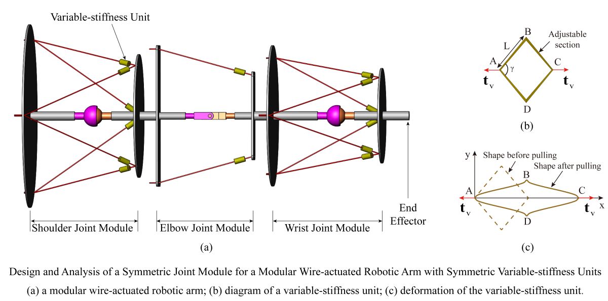
Inspired by the human arm, a wire-actuated robotic arm was designed in this paper, in which the rigid links were employed to instead of the skeleton of the human arm and the flexible steel wires were employed to instead of the muscles of the human arm. For the convenience of fabrication and maintenance, the wire-actuated robotic arm was made up of three joint modules: shoulder joint module, elbow joint module and wrist joint module. The three joint modules were connected in series to build a modular wire-actuated robot arm, as shown in Figure 1. The end of each wire for the robotic arm was connected with the wire actuation unit. All the wire actuation units were installed on the base of the robotic arm. This arrangement could reduce the moment of inertia and improve the security of the robot.
The three joint modules of the modular wire-actuated robotic arm could be divided into two types: one-degree-of-freedom (1-DOF) joint module and three-degree-of-freedom (3-DOF) joint module. The conceptual design of the 1-DOF and 3-DOF joint module were shown in Figure 2. The 1-DOF joint module had symmetric structure and consisted of a movable platform, a static platform, a revolute joint, and wires. The 3-DOF joint module consisted of a movable platform, a static platform, a spherical joint, and wires. Since the variation range of the steel wire was limited, a variable-stiffness unit (VSU) was developed and placed along the wire to raise the variable-stiffness range of the robotic arm and improve its flexibility and safety.
However, the existing VSUs generally had complex structure, large volume, heavy mass, and highly nonlinear stiffness-force relationship. In order to overcome these disadvantages, a novel VSU was proposed based on the flexure in this paper. As shown in Figure 3, the proposed VSU had simple, symmetric and compact structure. The VSU had a rhombus frame, denoted by ABCD. When the force acted at the point A and C, the VSU would deform. Due to the symmetric structure, we only need to analyze the deformation behavior of one side of the VSU. In this paper, the finite element method was employed to analyze the deformation of the VSU. The deformations of one side of the VSU were investigated under different forces. The results of the finite element analysis were shown in Figure 4.
Based on the FEA results, the stiffness-force relationship of the VSU yielded the following fitted function
where was the VSU stiffness, was the force acted on the VSU. The curve of the fitted function was shown in Figure 5, which had lowly nonlinear.
3. Kinematics Modelling and Analysis of the Symmetric Joint Module
In the 1-DOF joint module, the movable platform rotated around the center O of the revolute joint with respect to the static platform. Two coordinate systems were established at the center O of the revolute joint: the coordinate system {M} which was attached to the movable platform and the coordinate system {S} which was attached to the static platform. When the two coordinate systems coincided with each other, the joint module was said to be in the home pose, also known as the initial pose.
Based on the two coordinate systems, the pose of the movable platform relative to the static platform could be described by the pose of the coordinate system {M} relative to the coordinate system {S}, which could be expressed mathematically by the rotation matrix . Here represented Special Orthogonal group. Since the 1-DOF joint module had only one rotational degree of freedom, and the rotation only occurred in the plane of the coordinate system {S}, the pose of the movable platform relative to the static platform could be described by the rotational angle about the X axis of {S}. That meant the rotation matrix could be determined by only one parameter , which satisfied:
When the 1-DOF joint module was in the home pose, . When the movable platform rotated in the positive direction of the X axis, . When the movable platform rotated in the negative direction of the X axis, .
Writing as the distance of two points and , and as the distance of two points and , then for a given 1-DOF joint module, the parameters and were constant. Writing as the angle between the two lines and , when the 1-DOF joint module was in the home pose, the initial value of was written as , which satisfied
For a given 1-DOF joint module, was constant. When the movable platform rotated by the angle from the home pose, yielded:
Writing as the wire length between two points and , then the parameters and yielded:
Substituting (4) and (5) into (6), then the wire length satisfied the following equations when the movable platform rotated by the angle from the home pose, i.e.,
From (7) and (8), it could be concluded that the wire length was determined by the angle . On the other hand, the desired pose of the 1-DOF joint module could be reached by controlling the wire length .
Differentiating on both sides of (7) and (8), we had the following results:
Writing , where was the wire lengths of the 1-DOF joint module, then (9) and (10) could be written in the following matrix form:
Here was the Jacobian matrix, which yielded:
Writing as the angular velocity of the coordinate system {M} relative to the coordinate system {S} about the X axis of {S}, then (11) could be written as:
From (13), for a given pose of the 1-DOF joint module, the change rate of the wire lengths, , was determined by the angular velocity, . On the other hand, the rotational velocity could be adjusted by controlling the change rate of the wire lengths.
Based on the parameters and in the plane of coordinate system {S}, the angle vector and angular velocity of the 1-DOF joint module in coordinate system {S} could be written as following
According to the exponential formula, the rotation matrix of {M} relative to {S} could be written as following
where the operator was defined by
Then, in the coordinate system {S}, (13) could be expressed as following
where the Jacobian matrix yielded:
For a given pose of the 1-DOF joint module, the Jacobian matrix was constant. From (18), for a given pose of the 1-DOF joint module, the change rate of the wire lengths, , was determined by the angular velocity, . On the other hand, the rotational velocity could be adjusted by controlling the change rate of the wire lengths.
4. Stiffness Modelling and Analysis of the Symmetric Joint Module
As shown in Figure 6, the external force and torque acted on the movable platform of the 1-DOF joint module were denoted as and , the tension of the wire was denoted as , the force and torque acted on the revolute joint of the movable platform were denoted as and , respectively. In the coordinate system {S}, the movable platform of the 1-DOF joint module satisfied the following equilibrium equations
where .
Writing and defining as the unit vector along the wire of the 1-DOF joint module, then the tension of the wire could be written as
where represented the value of the wire tension . Thus the equilibrium equations (20) and (21) could be written as:
where was a vector composed of the values of the wire tension , and was a matrix composed of the unit vector , represented the Jacobian matrix and its transposed matrix yielded:
In this paper, the friction of the revolute joint was not considered. Then the component of the torque in the X-axis direction, denoted as , yielded
In the OYZ plane of the coordinate system {S}, (24) could be written as
where represented the component of the torque in the X-axis direction.
That was
where was given in (12).
When the component of torque acted on the movable platform of 1-DOF joint module increased from to , the movable platform would rotate slightly around the X axis of {S}, and the increment of the angular displacement would be denoted as . The torque increment and the angular increment yielded:
where represented the stiffness of the 1-DOF joint module around the X axis of {S}.
Differentiating on both sides of (28), it yielded:
Writing as:
where was defined as:
Substituting (12) into (32), it yielded:
In addition, according to (11), we had:
Then could be written as:
where . Here, represented the stiffness of the wire with the VSU in series. Since the stiffness of the wire was far greater than the stiffness of the VSU, then , where was the stiffness of the VSU placed in the wire.
Substituting (31) and (35) into (30), it yielded:
Then the stiffness of the 1-DOF joint module around the X axis of {S}, , could be written as
For a certain pose of the 1-DOF joint module, the matrix was constant. According to (28), when the component of the external torque, , was given and one of the wire tension was determined, another wire tension could be calculated. According to (37), the stiffness of the 1-DOF joint module could be adjusted by controlling the wire tensions.
5. Wire Tension Analysis of the Symmetric Joint Module
Since the wire could only pull, but not push, the wire-actuated joint module was actuated redundantly. According to the kinematics and stiffness analysis of the 1-DOF joint module, the wires of the 1-DOF joint module could be divided into two groups. Each group included one wire. The pose of the 1-DOF joint module could be adjusted by controlling the length of one wire, and the stiffness of the 1-DOF joint module could be adjusted by controlling the tension of another wire. It meant that the pose and stiffness of the 1-DOF joint module could be controlled synchronously. For a desired pose of the 1-DOF joint module, , the corresponding wire lengths could be solved from (7) and (8) easily. For a desired stiffness of the 1-DOF joint module, , the issue of finding out the corresponding wire tensions was called stiffness-oriented wire tension distribution (SWTD) problem.
According to the stiffness model (37) of the 1-DOF joint module, the desired stiffness yielded:
According to the equilibrium equation (28) of the 1-DOF joint module, when the pose and external force were given, and were both constant. The wire tension could be expressed by a function of the wire tension , i.e.,
Substituting (39) into (38), we had a quadratic equation with one variable . Solving from the quadratic equation and substituting into (39), the wire tension could be obtained. Then the two wire tensions and were both found out for the desired stiffness . That meant the SWTD problem of the 1-DOF joint module was solved.
In order to avoid the actuation wire be slack, a lower limit of the wire tension was set. In order to avoid the tension of the actuation wire exceeding the capacity of the wire driving unit and the VSU, an upper limit of the wire tension was set. In this paper, we set , . The solved wire tensions in the safe interval were called the feasible wire tensions.
6. Simulation Verification
To verify the proposed analysis and method, a simulation example was carried out. The 1-DOF joint module for simulation was shown in Figure 6, and its dimension parameters were given below:
(a) the distance between the wire hole and the center of the static platform:
(b) the distance between the wire hole and the center of the movable platform:
(c) the distance between the center of the static platform and the center O of the revolute joint:
(d) the distance between the center of the movable platform and the center O of the revolute joint:
Based on the dimension parameters of the 1-DOF joint module given above, the parameters , , could be calculated:
When the pose of the 1-DOF joint module, , was given, the parameters , could also be calculated according to (4), (5), (7) and (8), respectively.
In order to verify the solution to the SWTD problem of the 1-DOF joint module, two simulation cases were set for different poses and external loads of the 1-DOF joint module, named Case 1 and Case 2 respectively. For Case , two sub-cases were set for different desired stiffness, named Case -a and Case -b respectively. The cases of the simulation were listed in Table 1.
Here, we took Case 1-a as an example to illustrate the solution to the SWTD problem of the 1-DOF joint module. For the given pose , the parameters and could be calculated according to (33) and (12), respectively
Substituting and into (39), the wire tension could be obtained by the expression wire tension :
Substituting the desired stiffness and (45) into (38), a quadratic equation of was obtained:
Solving (46), we had the wire tension . Substituting into (45), we obtained the wire tension . The wire tension and were both in the safe interval . In summary, for Case 1-a, the feasible wire tensions for the desired stiffness were and .
Similar to Case 1-a, the wire tension solutions to the SWTD problem of the 1-DOF joint module for the other simulation cases could be obtained. The results of the simulation were listed in Table 1.
7. Conclusion
In this paper, a modular wire-actuated robotic arm was proposed to improve the safety and adaptability of service robots during human-robot interaction, which consisted of three symmetric joint modules in series. To raise the stiffness adjustment range of the robotic arm, a variable-stiffness unit (VSU) was designed based on flexure, which had simple, symmetric and compact structure. The FEA result shown that the VSU yielded lowly nonlinear stiffness-force relationship. In this paper, we focused on the research of the 1-DOF joint module, including kinematics, statics, stiffness and wire tension analysis. It shown that the pose of the joint module could be adjusted by controlling the length of the wires, and the stiffness of the joint module could be adjusted by controlling the tension of the wires. Due to the actuation redundancy, the wires could be divided into two groups, and the pose and stiffness of the joint module could be controlled synchronously. For a given desired stiffness, in order to find out the corresponding wire tensions, the stiffness-oriented wire tension distribution (SWTD) problem should be solved. In this paper, a directly method was proposed for the SWTD problem of the 1-DOF joint module. A simulation was carried out to verify the effectiveness of the proposed analysis and method.
Author Contributions
Conceptualization, K.Y.; formal analysis, K.Y., C.Q., Y.R., and J.H.; methodology, K.Y., C.Q., Y.R., and J.H.; validation, Z.S.; writing-original draft, C.Q.; writing-review and editing, C.W. and C.X.; supervision, K.Y. All authors have read and agreed to the published version of the manuscript.
Funding
This research was funded by Public Welfare Technology Research Program of Zhejiang Province, China (Grant number: LGF22E050003), Public Welfare Technology Research Program of Ningbo City, China (Grant number: 2022S130), Key Research and Development Program of Ningbo City, China (Grant number: 2022Z062).
Data Availability Statement
Data are contained with the article.
Conflicts of Interest
The authors declare no conflicts of interest.
References
- Tang, Y.; Zhang, Q.; Lin, G.; Yin, J. Switchable adhesion actuator for amphibious climbing soft robot. Soft Robot. 2018, 5, 592–600. [Google Scholar] [CrossRef] [PubMed]
- Tian, B.; Gao, H.; Yu, H.; Shan, H.; Hou, J.; Yu, H.; Deng, Z. Cable-driven legged landing gear for unmanned helicopter: Prototype design, optimization and performance assessment. Sci. China Technol. Sc. 2024, 67, 1196–1214. [Google Scholar] [CrossRef]
- Yoon, J.; Lee, D.; Bang, J.; Shin, H.G.; Chung, W.K.; Choi, S.; Kim, K. Cable-driven haptic interface with movable bases achieving maximum workspace and isotropic force exertion. IEEE T. Haptics 2023, 16, 365–378. [Google Scholar] [CrossRef] [PubMed]
- Mailhot, N.; Abouheaf, M.M.; Spinello, D. Model-free force control of cable-driven parallel manipulators for weight-shift aircraft actuation. IEEE T. Instrum. Meas. 2024, 73, 2505108. [Google Scholar] [CrossRef]
- Axinte, D.; Dong, X.; Palmer, D.; Rushworth, A.; Guzman, S.C.; Olarra, A.; Arizaga, I.; Gomez-Acedo, E.; Txoperena, K.; Pfeiffer, K.; Messmer, F.; Gruhler, M.; Kell, J. MiRoR-miniaturised robotic systems for holistic in-situ repair and maintenance works in restrained and hazardous environments. IEEE-ASME T. Mech. 2018, 23, 978–981. [Google Scholar] [CrossRef]
- Troncoso, D.A.; Robles-Linares, J.A.; Russo, M.; Elbanna, M.A.; Wild, S.; Dong, X.; Mohammad, A.; Kell, J.; Norton, A.D.; Axinte, D. A continuum robot for remote applications: From industrial to medical surgery with slender continuum robots. IEEE Robot. Autom. Mag. 2023, 30, 94–105. [Google Scholar] [CrossRef]
- Dong, X.; Wang, M.; Mohammad, A.; Ba, W.; Russo, M.; Norton, A.; Kell, J.; Axinte, D. Continuum robots collaborate for safe manipulation of high-temperature flame to enable repairs in challenging environments. IEEE-ASME T. Mech. 2022, 27, 4217–4220. [Google Scholar] [CrossRef]
- Choi H, C.; Kang, B.B.; Jung, B.; Cho, K.J. Exo-wrist: a soft tendon-driven wrist-wearable robot with active anchor for dart-throwing motion in hemiplegic patients. IEEE Robot. Autom. Let. 2019, 4, 4499–4506. [Google Scholar] [CrossRef]
- Pu, S.W.; Pei, Y.C.; Chang, J.Y. Decoupling finger joint motion in an exoskeletal hand: a design for robot-assisted rehabilitation. IEEE T. Ind. Electron. 2020, 67, 686–697. [Google Scholar] [CrossRef]
- Wang, X.; Guo, S.; Bai, S. A cable-driven parallel hip exoskeleton for high-performance walking assistance. IEEE-ASME T. Mech. 2024, 71, 2705–2715. [Google Scholar] [CrossRef]
- Xu, M.; Zhou, Z.; Wang, Z.; Wang, Z.; Ruan, L.; Mai, J.; Wang, Q. Bioinspired cable-driven actuation system for wearable robotic devices: Design, control, and characterization. IEEE T. Robot. 2024, 40, 520–539. [Google Scholar] [CrossRef]
- Liao, H.; Chan, H.H.; Liu, G.; Zhao, X.; Gao, F.; Tomizuka, M.; Liao, W.H. Design, control, and validation of a novel cable-driven series elastic actuation system for a flexible and portable back-support exoskeleton. IEEE T. Robot. 2024, 40, 2769–2790. [Google Scholar] [CrossRef]
- Nakka, S.; Vashista, V. External dynamics dependent human gait adaptation using a cable-driven exoskeleton. IEEE Robot. Autom. Let. 2023, 8, 6036–6043. [Google Scholar] [CrossRef]
- Wu, Z.; Li, Q.; Zhao, J.; Gao, J.; Xu, K. Design of a modular continuum-articulated laparoscopic robotic tool with decoupled kinematics. IEEE Robot. Autom. Let. 2019, 4, 3545–3552. [Google Scholar] [CrossRef]
- Rivas-Blanco, I.; Lopez-Casado, C.; Perez-Del-Pulgar, C.J.; García-Vacas, F.; Fraile, J.C.; Muñoz, V.F. Smart cable-driven camera robotic assistant. IEEE T. Hum-Mach Syst. 2018, 48, 183–196. [Google Scholar] [CrossRef]
- Wang, W.; Wang, J.; Chen, C.; Luo, Y.; Wang, X.; Yu, L. Design of position estimator for rope driven micromanipulator of surgical robot based on parameter autonomous selection model. J. Mech. Robot. 2024, 16, 041005. [Google Scholar] [CrossRef]
- Li, C.; Gu, X.; Ren, H. A cable-driven flexible robotic grasper with Lego-like modular and reconfigurable joints. IEEE-ASME T. Mech. 2017, 22, 2757–2767. [Google Scholar] [CrossRef]
- Kim, Y.J. Anthropomorphic low-inertia high-stiffness manipulator for high-speed safe interaction. IEEE T. Robot. 2017, 33, 1358–1374. [Google Scholar] [CrossRef]
- Xiao, H.; Tang, J.; Lyu, S.; Xu, K.; Ding, X. Design and implementation of a synergy-based cable-driven humanoid arm with variable stiffness. J. Mech. Robot. 2024, 16, 041002. [Google Scholar] [CrossRef]
- Lin, B.; Xu, W.; Li, W.; Yuan, H.; Liang, B. Ex situ sensing method for the end-effector’s six-dimensional force and link’s contact force of cable-driven redundant manipulators. IEEE T. Ind. Inform. 2024, 20, 7995–8006. [Google Scholar] [CrossRef]
- Li, R.; Liu, Y.; Guo, A.; Shou, M.; Zhao, M.; Zhu, D.; Yang, P.; Lee, C.H. An inchworm-like climbing robot based on cable-driven grippers. IEEE-ASME T. Mech. 2024, 29, 1591–1600. [Google Scholar] [CrossRef]
- Xu, W.; Liu, T.; Li, Y. Kinematics, dynamics, and control of a cable-driven hyper-redundant manipulator. IEEE-ASME T. Mech. 2018, 23, 1693–1704. [Google Scholar] [CrossRef]
- Wu, L.; Crawford, R.; Roberts, J. Dexterity analysis of three 6-DOF continuum robots combining concentric tube mechanisms and cable-driven mechanisms. IEEE Robot. Autom. Let. 2017, 2, 514–521. [Google Scholar] [CrossRef]
- Yang, Q.; Zhou, Q.; Zhou, G.; Jiang, M.; Zhao, Z. Inverse kinematics solution method of an adaptive piecewise geometry for cable-driven hyper-redundant manipulator. J. Mech. Robot. 2024, 16, 041011. [Google Scholar] [CrossRef]
- Dai, Y.; Wang, S.; Wang, X.; Yuan, H. A novel friction measuring method and its application to improve the static modeling accuracy of cable-driven continuum manipulators. IEEE Robot. Autom. Let. 2024, 9, 3259–3266. [Google Scholar] [CrossRef]
- Yang, H.; Xia, C.; Wang, X.; Xu, W.; Liang, B. An efficient solver for the inverse kinematics of cable-driven manipulators with pure rolling joints using a geometric iterative approach. Mech. Mach. Theory 2024, 196, 105611. [Google Scholar] [CrossRef]
- Lau, D.; Eden, J.; Oetomo, D.; Halgamuge, K.S. Musculoskeletal static workspace analysis of the human shoulder as a cable-driven robot. IEEE-ASME T. Mech. 2015, 20, 978–984. [Google Scholar] [CrossRef]
- Cheng, H.H.; Lau, D. Cable attachment optimization for reconfigurable cable-driven parallel robots based on various workspace conditions. IEEE T. Robot. 2023, 39, 3759–3775. [Google Scholar] [CrossRef]
- Haghighipanah, M.; Miyasaka, M.; Hannaford, B. Utilizing elasticity of cable-driven surgical robot to estimate cable tension and external force. IEEE Robot. Autom. Let. 2017, 2, 1593–1600. [Google Scholar] [CrossRef]
- Jamshidifar, H.; Khajepour, A.; Fidan, B.; Rushton, M. Kinematically-constrained redundant cable-driven parallel robots: Modeling, redundancy analysis, and stiffness optimization. IEEE-ASME T. Mech. 2017, 22, 921–930. [Google Scholar] [CrossRef]
- Xu, G.; Zhu, H.; Xiong, H.; Lou, Y. Data-driven dynamics modeling and control strategy for a planar n-DOF cable-driven parallel robot driven by n+1 cables allowing collisions. J. Mech. Robot. 2024, 16, 051008. [Google Scholar] [CrossRef]
- Mamidi, T.K.; Bandyopadhyay, S. A modular computational framework for the dynamic analyses of cable-driven parallel robots with different types of actuation including the effects of inertia, elasticity and damping of cables. Robotica 2024, 42, 1676–1708. [Google Scholar] [CrossRef]
- Zhang, Z.; Cheng, H.H.; Lau, D. Efficient wrench-closure and interference-free conditions verification for cable-driven parallel robot trajectories using a ray-based method. IEEE Robot. Autom. Let. 2020, 5, 8–15. [Google Scholar] [CrossRef]
- Ding, M.; Zheng, X.; Liu, L.; Guo, J.; Guo, Y. Collision-free path planning for cable-driven continuum robot based on improved artificial potential field. Robotica 2024, 42, 1350–1367. [Google Scholar] [CrossRef]
- Qin, Y.; Chen, Q.; Ming, C. Adaptive recursive sliding mode based trajectory tracking control for cable-driven continuum robots. ISA T. 2024, 147, 501–510. [Google Scholar] [CrossRef]
- Han, Z.; Liu, Z.; Meurer, T.; He, W. PDE-based control synthesis for a planar cable-driven continuum arm. Automatica 2024, 163, 1116000. [Google Scholar] [CrossRef]
- Ameri, A.; Molaei, A.; Khosravi, M.A.; Aghdam, A.G.; Javad Dargahi, J.S.; Fazeli, M. A real-time approach to risk-free control of highly redundant cable-driven parallel robots. IEEE T. Syst. Man Cy-S. 2024, 54, 2651–2662. [Google Scholar] [CrossRef]
- Cheah, S.K.; Hayes, A.; Caverly, R.J. Adaptive passivity-based pose tracking control of cable-driven parallel robots for multiple attitude parameterizations. IEEE T. Contr. Syst. T. 2024, 32, 202–213. [Google Scholar] [CrossRef]
- Li, W.; Huang, X.; Yan, L.; Cheng, H.; Liang, B.; Xu, W. Force sensing and compliance control for a cable-driven redundant manipulator. IEEE-ASME T. Mech. 2024, 29, 777–788. [Google Scholar] [CrossRef]
- Zhang, B.; Shang, W.; Deng, B.; Shuang Cong, S.; Li, Z. High-precision adaptive control of cable-driven parallel robots with convergence guarantee. IEEE T. Ind. Electron. 2024, 71, 7370–7380. [Google Scholar] [CrossRef]
- Yang, K.; Chen, C.; Ye, D.; Wu, K.; Zhang, G. Stiffness modelling and distribution of a modular cable-driven human-like robotic arm. Mech. Mach. Theory 2023, 180, 105150. [Google Scholar] [CrossRef]
- Chen, W.; Fang, X.; Che, J.; Xiong, C. Design and analysis of passive variable stiffness device based on shear stiffening gel. Smart Mater. Struct. 2022, 31, 125007. [Google Scholar] [CrossRef]
- Zhu, Y.; Wu, Q.; Chen, B.; Xu, D.; Shao, Z. Design and evaluation of a novel torque-controllable variable stiffness actuator with reconfigurability. IEEE-ASME T. Mech. 2022, 27, 292–303. [Google Scholar] [CrossRef]
- Zhao, Y.; Chen, K.; Yu, J.; Huang, S. Design of a parallel compliance device with variable stiffness. P. I. Mech. Eng. C-J Mec. 2021, 235, 94–107. [Google Scholar] [CrossRef]
- Yang, K.; Yang, G.; Zhang, C.; Chen, C.; Zheng, T.; Cui, Y.; Chen, T. Cable tension analysis oriented the enhanced stiffness of a 3-DOF joint module of a modular cable-driven human-like robotic arm. Appl. Sci-Basel 2020, 10, 8871. [Google Scholar] [CrossRef]
Figure 1.
Conceptual design of the modular wire-actuated robotic arm.
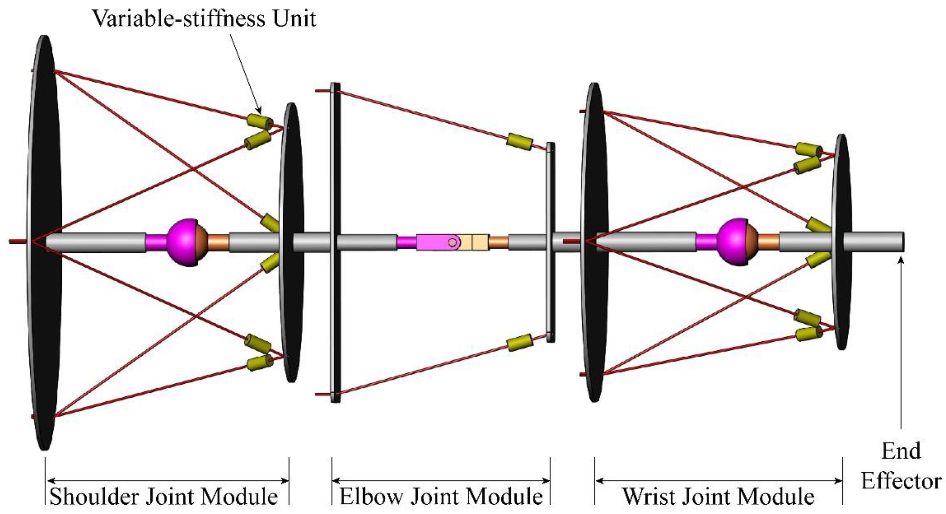
Figure 2.
Conceptual design of joint modules: (a) 1-DOF joint module; (b) 3-DOF joint module.
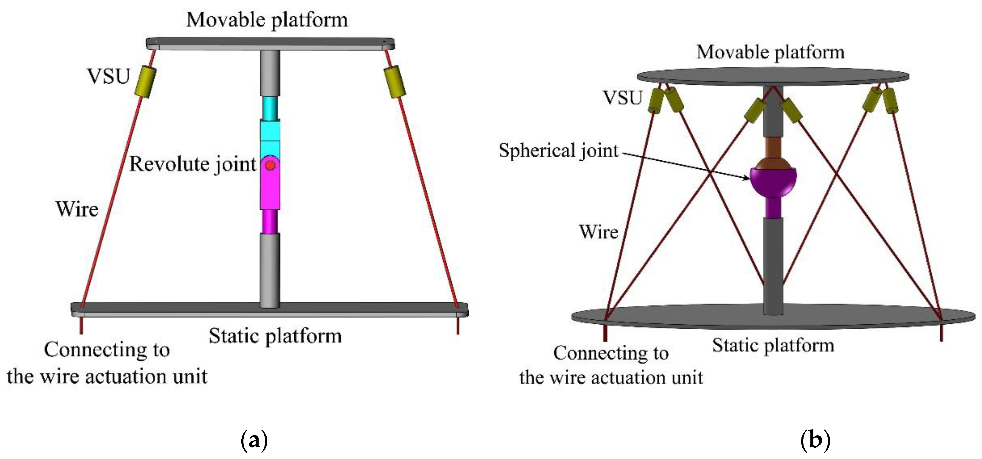
Figure 3.
Design of the variable-stiffness unit (VSU): (a) diagram of the VSU; (b) deformation of the VSU after pulling.
Figure 3.
Design of the variable-stiffness unit (VSU): (a) diagram of the VSU; (b) deformation of the VSU after pulling.
Figure 4.
FEA for one side of the VSU under different loads: (a) ; (b) ; (c) ; (d) ; (e) ; (f) ; (g) ; (h) ; (i) .
Figure 4.
FEA for one side of the VSU under different loads: (a) ; (b) ; (c) ; (d) ; (e) ; (f) ; (g) ; (h) ; (i) .
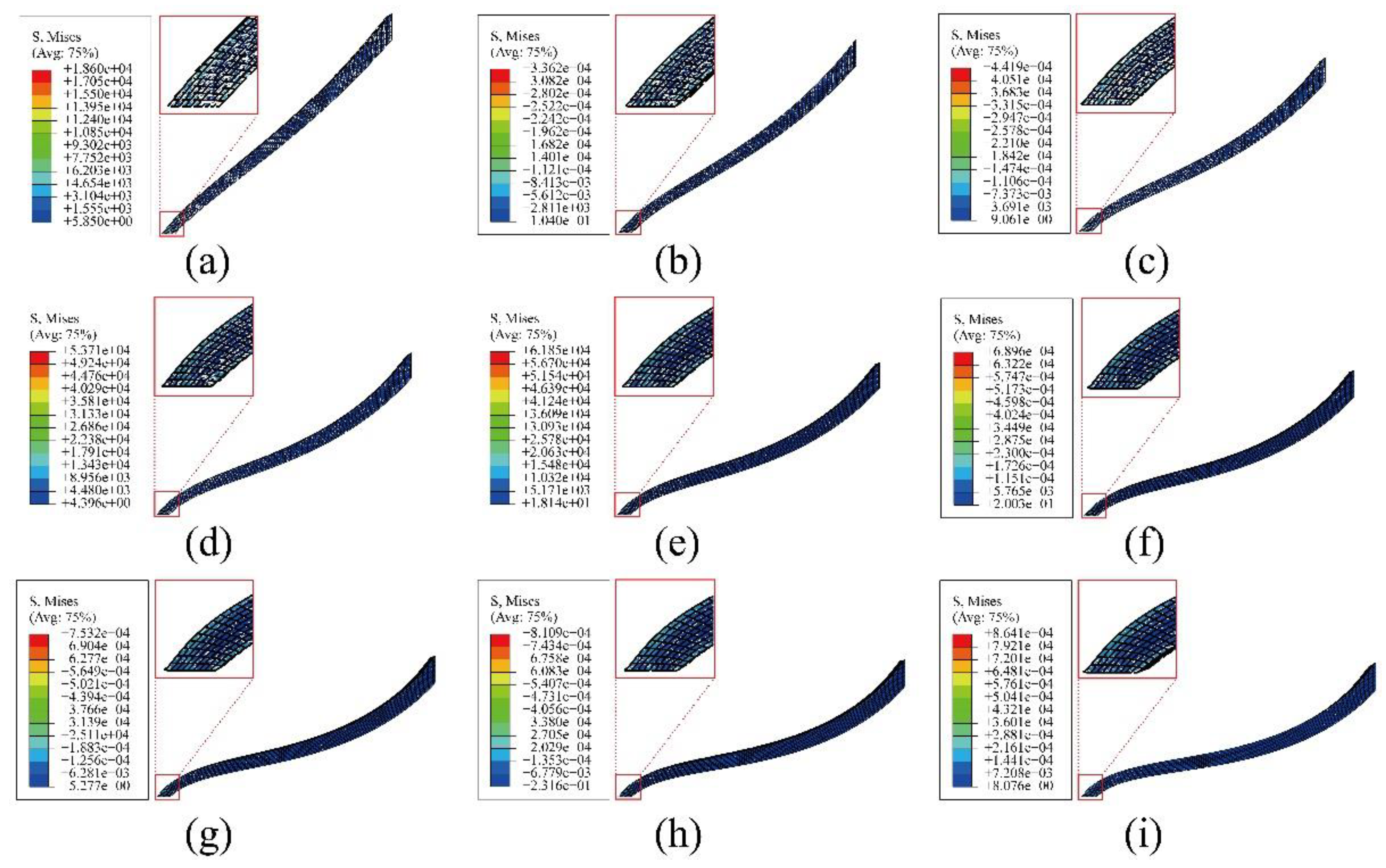
Figure 5.
Stiffness-force relationship of the VSU.
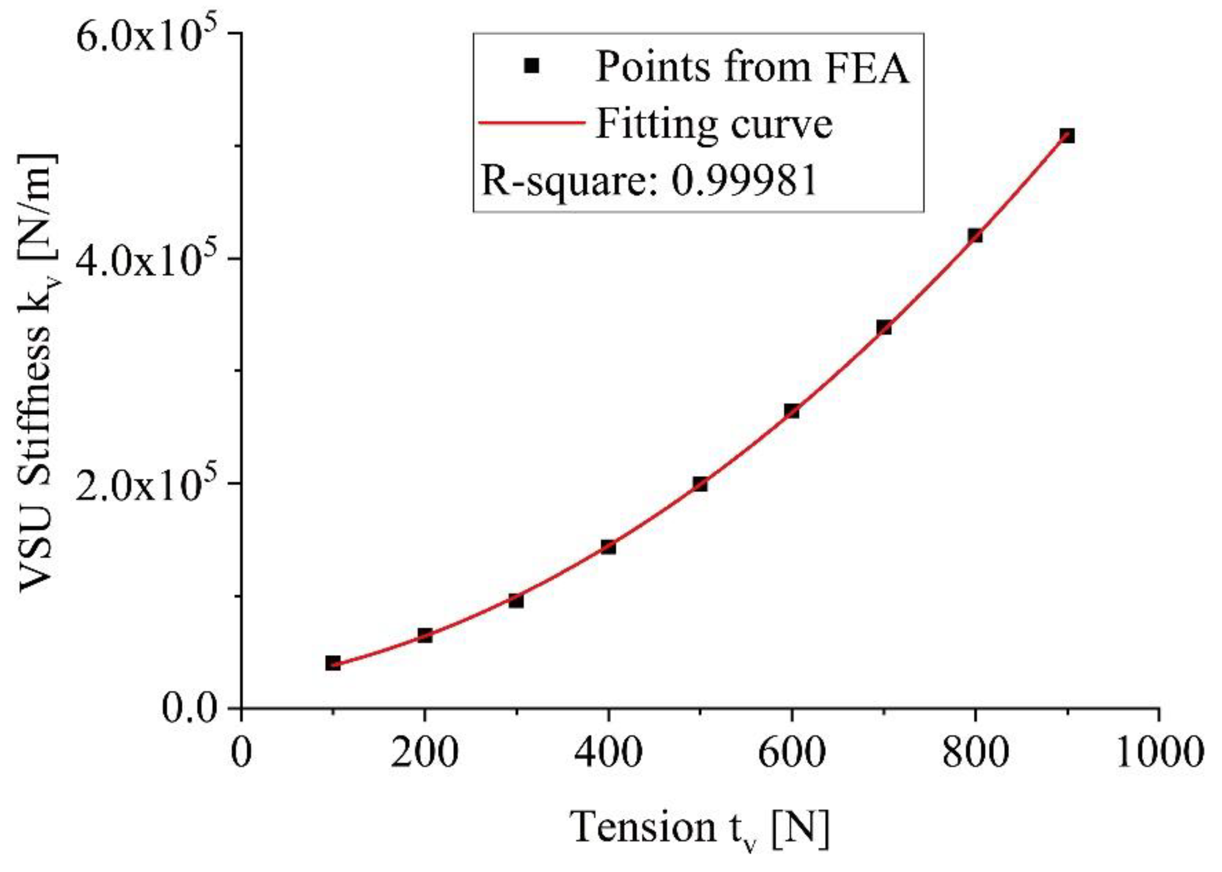
Figure 6.
Diagram of the 1-DOF joint module.
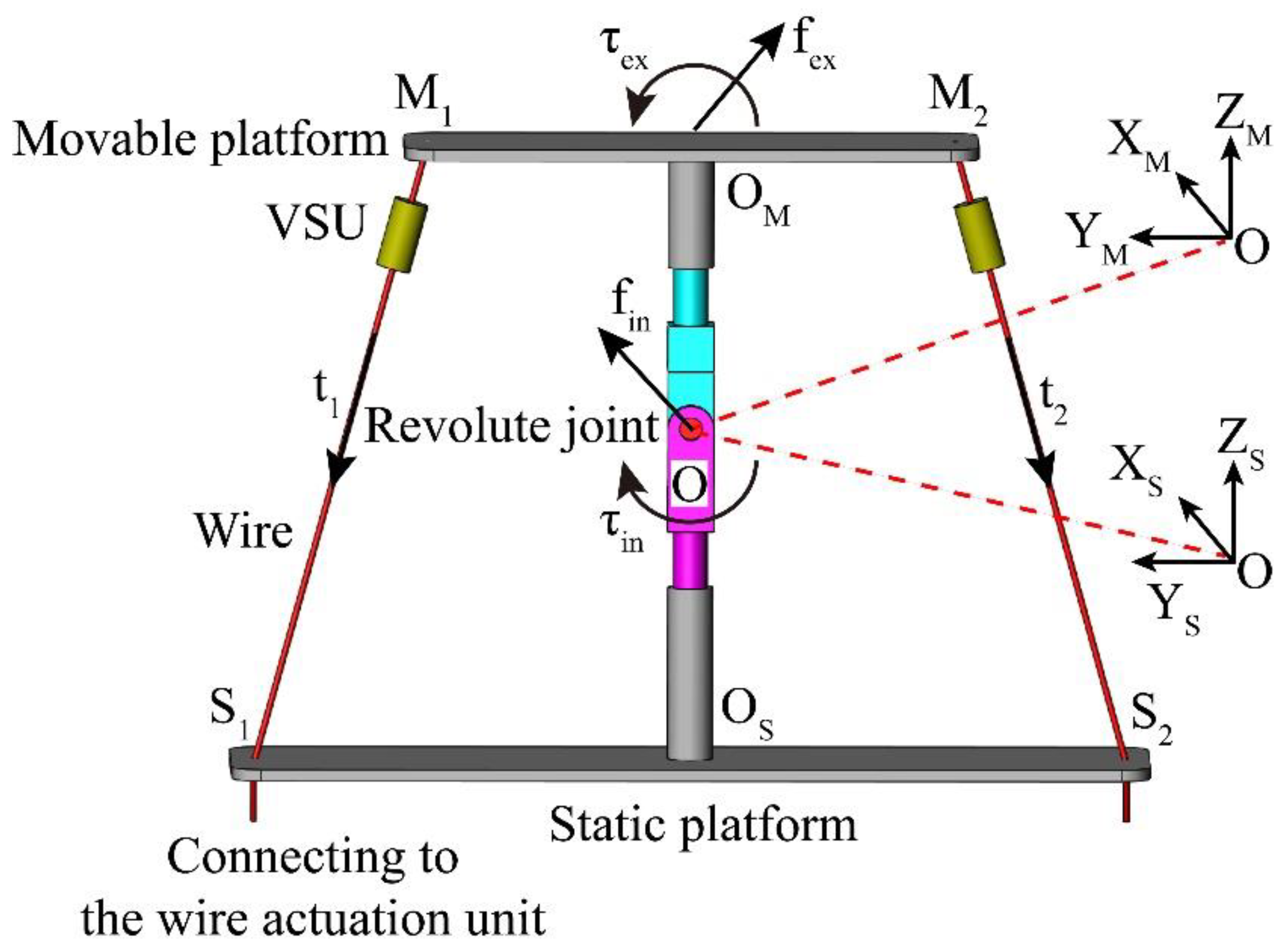

Table 1.
Simulation cases for the SWTD problem of the 1-DOF joint module.
| Case | External loads (Nm) |
Pose (rad) |
Desired stiffness (Nm/rad) |
Wire tension (N) |
|---|---|---|---|---|
| Case 1-a | 2 | 0.0524 | 368.66 | |
| Case 1-b | 2 | 0.0524 | 315.14 | |
| Case 2-a | -2 | 0.0349 | 324.25 | |
| Case 2-b | -2 | 0.0349 | 291.54 |
Disclaimer/Publisher’s Note: The statements, opinions and data contained in all publications are solely those of the individual author(s) and contributor(s) and not of MDPI and/or the editor(s). MDPI and/or the editor(s) disclaim responsibility for any injury to people or property resulting from any ideas, methods, instructions or products referred to in the content. |
© 2024 by the authors. Licensee MDPI, Basel, Switzerland. This article is an open access article distributed under the terms and conditions of the Creative Commons Attribution (CC BY) license (http://creativecommons.org/licenses/by/4.0/).
Copyright: This open access article is published under a Creative Commons CC BY 4.0 license, which permit the free download, distribution, and reuse, provided that the author and preprint are cited in any reuse.


