Analyzing the Approximate Error and the Applicable Condition of Fractional Reduced Differential Transform Method

Preprint

Article

Analyzing the Approximate Error and the Applicable Condition of Fractional Reduced Differential Transform Method

Altmetrics

Downloads

Views

Comments

A peer-reviewed article of this preprint also exists.

Jianbing Hu^*

This version is not peer-reviewed

Submitted:

16 May 2024

Posted:

17 May 2024

You are already at the latest version

Alerts

Abstract

The fractional reduced differential transform method is a finite iterative method based on infinite fractional expansions. The result obtained is the approximation of the real value. There are few reports on the approximate error and the applicable condition. In this paper, according to the fractional expansions, we study the factors related to the approximate errors. Our research shows that the approximate errors relate not only to fractional order but also to time $t$ and increase rapidly with time $t$. This method can only be applied within a certain time range and the time range is relevant to fractional order and fractional expansions. Then, many obtained achievements may be incorrect if the applicable conditions are not satisfied. Some examples presented in this paper verify our analysis.

Keywords:

Subject: Computer Science and Mathematics - Applied Mathematics

MSC: 00-01; 99-00

1. Introduction

Fractional calculus is an extension of integer calculus from integer dimension to fractional dimension, and can be applied to depict real physical systems with arbitrary accuracy. Fractional models are treated in many areas such as signal processing[1], image processing, control engineering[2], mechanic engineering etc[3,4,5,6].

The fractional calculus is defined by a convolution operation and is computationally complex. How to simplify this computation is an important research topic in the fractional field. Many approximate approaches have been proposed for this issue [7,8,9,10,11,12]. Without exception, only an approximation solution, but not an exact solution, can be obtained by any approximate method. There must exist an approximate error between the approximate solution and the exact solution. Only within the allowable range of the approximate error can this approximate method be correct. Or else, the achievements obtained may be incorrect[13,14,15]. For example, Ahmadian A. obtained the approximate solution in the time domain by its approximate value in Laplace domain[12], but Zhao L. etc[16] analyzed the approximate error and pointed out that this approach may mislead.

Similarly, fractional reduced differential transform method is also an approximate approach, and the approximate value is obtained by omitting some high order items of fractional expansions. It has been applied to solve fractional partial differential equations [17,18,19], higher-dimensional fractional equation[20], fractional nonlinear equation[21], fractional transport model[22], fractional financial models of awareness[23,24] etc. By this approach, the calculating process can be simplified and the approximate value can be drawn when the omitted high-order items are infinitesimal, but it can also mislead when the omitted high-order items are not infinitesimal. On the other hand, the high-order terms that are ignored may be infinitesimal within a certain time range and gradually increase over this time range. This method can only be applied in a certain time range. However, the approximate error and the applicable condition have rarely been reported in the obtained achievements. Some special examples presented cannot verify the effectiveness of the mentioned method.

In this paper, we study the fractional expansion and obtain its parameters according to the mean value theorem. The parameters are drawn step by step based on the hypothesis that the high-order items are infinitesimal. Then, we draw the applicable condition from the allowable error. Some examples are taken to verify our analysis. Numerical simulations show that the approximate error is convergent in a certain time range and increases rapidly over this time range.

The rest of this paper is organized as follows. Section 2 addresses the definitions and some properties of fractional calculus. Fractional reduced differential transform method is formulated in Section 3. We analyze the approximate error and the applicable condition in Section 4. In Section 5, some examples are taken to verify our analysis. Lastly, a conclusion is drawn in Section 6.

2. The Definitions and Some Properties of Fractional Calculus

There exist many fractional derivative definitions, among which the Caputo fractional derivative definition is widely adapted as it is irrelevant to the initial condition. In this paper, the Caputo fractional derivative definition is adapted.

Definition 1.

The fractional derivative in the Caputo sense of the function

ς (t) \in C^{n} (t \in [t_{0}, + \infty), R)

with order ϵ is defined as

\begin{matrix} _{t_{0}}^{C} D_{t}^{ϵ} ς (t) & = \frac{1}{Γ (n - ϵ)} \int_{t_{0}}^{t} \frac{ς^{(n)} (τ)}{{(t - τ)}^{ϵ - n + 1}} d τ \end{matrix}

(1)

where

Γ (\cdot)

is the Gamma function,

ς (t_{0})

is the initial value of

ς (t)

and n is a positive integer such that

n - 1 < ϵ < n

Definition 2.

The fractional integral of function

ς (t)

with order ϵ is defined as

\begin{matrix} _{t_{0}} I_{t}^{ϵ} ς (t) & = \frac{1}{Γ (ϵ)} \int_{t_{0}}^{t} {(t - τ)}^{ϵ - 1} ς (τ) d τ \end{matrix}

(2)

Some properties of fractional calculus that may be adapted are introduced in the following.

(i)

For a continuous function

ς (t)

_{t_{0}} I_{t}^{ϵ} [_{t_{0}}^{C} D_{t}^{ϵ} ς (t)] = ς (t) - ς (t_{0})

(i i)

_{t_{0}}^{C} D_{t}^{ϵ} C = 0

, where C is a constant.

(i i i)

_{t_{0}}^{C} D_{t}^{ϵ} t^{ξ} = \frac{Γ (ξ + 1)}{Γ (ξ - ϵ + 1)} {(t - t_{0})}^{ξ - ϵ}

, where

n - 1 < ϵ < n

and

ϵ

is not an integer less than n.

(i v)

_{t_{0}}^{C} D_{t}^{α} (_{t_{0}}^{C} D_{t}^{ϵ} ς (t)) =_{t_{0}}^{C} D_{t}^{α + ϵ} ς (t)

Theorem 1.

ς^{(n)} (t) (t \in [t_{0}, a])

is a continuous function, there must exist a constant

ν \in [t_{0}, a]

satisfying

\begin{matrix} _{t_{0}}^{C} D_{t}^{ϵ} ς (t) = \frac{ς^{(n)} (ν)}{Γ (n - ϵ + 1)} {(t - t_{0})}^{n - ϵ} \end{matrix}

(3)

Proof.

According to the mean value theorem, there must exist

ν \in [t_{0}, a]

satisfying the following equation,

\begin{matrix} _{t_{0}}^{C} D_{t}^{ϵ} ς (t) = \frac{1}{Γ (n - ϵ)} \int_{t_{0}}^{t} \frac{ς^{(n)} (τ)}{{(t - τ)}^{ϵ - n + 1}} {d τ |}_{t = a} \\ = ς^{(n)} (ν) \frac{1}{Γ (n - ϵ)} \int_{t_{0}}^{t} \frac{1}{{(t - τ)}^{ϵ - n + 1}} d τ \\ = \frac{ς^{(n)} (ν)}{Γ (n - ϵ + 1)} {(t - t_{0})}^{n - ϵ} \end{matrix}

(4)

where

m i n (ς^{(n)} (t)) \leq ς^{(n)} (ν) \leq m a x (ς^{(n)} (t))

The proof of Theorem 1 is completed. □

Conclusion 1: If

ς (t) (t \in [t_{0}, a])

is a continuous function, there must exist a constant

ν \in [t_{0}, a]

satisfying

_{t_{0}} I_{t}^{ϵ} ς (t) ∣_{t = a} = ς (ν) \frac{1}{Γ (ϵ)} \int_{t_{0}}^{t} {(t - τ)}^{ϵ - 1} d τ

Note 1: Especially, when

t \to t_{0}

, it yields

ς^{(n)} (ν) = ς^{(n)} (t_{0}) = ς^{(n)} (t)

and

\begin{matrix} lim_{t \to t_{0}}_{t_{0}}^{C} D_{t}^{ϵ} ς (t) = \frac{ς^{(n)} (t_{0})}{Γ (n - ϵ + 1)} {(t - t_{0})}^{n - ϵ} \end{matrix}

(5)

Obviously, the above holds only when

t \to t_{0}

. Or else, it may be incorrect.

Theorem 2.

When

0 < ϵ \leq 1

, if

ς (t)

and

g (t)

(

t \in (t_{0}, t_{b})

) are continuous differentiable functions, there must exist a constant

ν \in [t_{0}, t_{b}]

making the following equation hold,

\begin{matrix} \frac{ς (t_{b}) - ς (t_{0})}{g (t_{b}) - g (t_{0})} = \frac{_{t_{0}}^{C} D_{t}^{ϵ} {ς (t) |}_{t = ν}}{_{t_{0}}^{C} D_{t}^{ϵ} {g (t) |}_{t = ν}} \end{matrix}

(6)

Proof.

Define function

ϑ (t) = ς (t) - \frac{ς (t_{b}) - ς (t_{0})}{g (t_{b}) - g (t_{0})} g (t)

and get

\begin{matrix} ϑ (t_{b}) - ϑ (t_{0}) = 0 \end{matrix}

(7)

From the property of fractional calculus, it yields

\begin{matrix} ϑ (t_{b}) - ϑ (t_{0}) \\ =_{t_{0}} I_{t}^{ϵ} [_{t_{0}}^{C} D_{t}^{ϵ} ϑ (t)] \\ = \frac{1}{Γ (ϵ)} \int_{t_{0}}^{t} {(t - τ)}^{ϵ - 1} [_{t_{0}}^{C} D_{τ}^{ϵ} ϑ (τ)] d τ \end{matrix}

(8)

According to Conclusion 1, we obtain

\begin{matrix} ϑ (t_{b}) - ϑ (t_{0}) \\ = \frac{1}{Γ (ϵ)} \int_{t_{0}}^{t} {(t - τ)}^{ϵ - 1} [_{t_{0}}^{C} D_{τ}^{ϵ} ϑ (τ)] d τ \\ = [_{t_{0}}^{C} D_{t}^{ϵ} ϑ (t)] |_{t = ν} \frac{1}{Γ (ϵ)} \int_{t_{0}}^{t} {(t - τ)}^{ϵ - 1} d τ \\ = 0 \end{matrix}

(9)

Then, there must exist a constant

ν \in [t_{0}, a]

satisfying

\begin{matrix} [_{t_{0}}^{C} D_{t}^{ϵ} ϑ (t)] {|_{t = ν} =_{t_{0}}^{C} D_{t}^{ϵ} [ς (t) - \frac{ς (t_{b}) - ς (t_{0})}{g (t_{b}) - g (t_{0})} g (t)] |}_{t = ν} \\ = [_{t_{0}}^{C} D_{t}^{ϵ} ς (t) - \frac{ς (t_{b}) - ς (t_{0})}{g (t_{b}) - g (t_{0})}_{t_{0}}^{C} D_{t}^{ϵ} g (t)] |_{t = ν} \\ = 0 \end{matrix}

(10)

We can obtain

\begin{matrix} \frac{ς (t_{b}) - ς (t_{0})}{g (t_{b}) - g (t_{0})} = \frac{_{t_{0}}^{C} D_{t}^{ϵ} {ς (t) |}_{t = ν}}{_{t_{0}}^{C} D_{t}^{ϵ} {g (t) |}_{t = ν}} \end{matrix}

(11)

The proof of Theorem 2 is completed. □

Theorem 3.

ς (t)

and

g (t)

are continuous differentiable functions satisfying

lim_{t \to t_{0}} ς (t) = 0

and

lim_{t \to t_{0}} g (t) = 0

, the following equation holds

\begin{matrix} lim_{t \to t_{0}} \frac{ς (t)}{g (t)} = lim_{t \to t_{0}} \frac{_{t_{0}}^{C} D_{t}^{ϵ} ς (t)}{_{t_{0}}^{C} D_{t}^{ϵ} g (t)} \end{matrix}

(12)

where

0 < ϵ \leq 1

Proof.

lim_{t \to t_{0}} ς (t) = 0

and

lim_{t \to t_{0}} g (t) = 0

, we set

ς (t_{0}) = 0

and

g (t_{0}) = 0

. According to Theorem 2, it gets

\begin{matrix} lim_{t \to t_{0}} \frac{ς (t)}{g (t)} = lim_{t \to t_{0}} \frac{ς (t_{b}) - ς (t_{0})}{g (t_{b}) - g (t_{0})} = lim_{t \to t_{0}} \frac{_{t_{0}}^{C} D_{t}^{ϵ} ς (t)}{_{t_{0}}^{C} D_{t}^{ϵ} g (t)} \end{matrix}

(13)

The proof of Theorem 3 is completed. □

3. Fractional Reduced Differential Transform Method

Suppose

ς (t)

is a continuous and differentiable function. This function can be embodied as

\begin{matrix} ς (t) = \sum_{k = 0}^{\infty} V_{k ϵ} {(t - t_{0})}^{k ϵ} \end{matrix}

(14)

where

0 < ϵ \leq 1

V_{k ϵ}

represents the spectrum of function

ς (t)

Usually, we can only calculate finite but not infinite items. Then, many items will be omitted and equation (14) can be expressed as

\begin{matrix} ς (t) = \sum_{k = 0}^{j} V_{k ϵ} {(t - t_{0})}^{k ϵ} + o {((t - t_{0}))}^{k ϵ} \end{matrix}

(15)

When t is within the neighborhood of

t_{0}

o {((t - t_{0}))}^{k ϵ}

is the

k ϵ

order infinitesimal of

(t - t_{0})

. Then, we can obtain the approximate

{\tilde{ς}}_{j} (t)

ς (t)

\begin{matrix} {\tilde{ς}}_{k} (t) = \sum_{k = 0}^{j} V_{k ϵ} {(t - t_{0})}^{k ϵ} \end{matrix}

(16)

Obviously, the approximate error decreases with j increasing.

Based on the above hypothesis, when

0 < ϵ < 1

, let us study the expression of

V_{k ϵ}

step by step.

When

k = 0

, it has

\begin{matrix} lim_{t \to t_{0}} ς (t) = V_{ϵ 0} {(t - t_{0})}^{0} + o {((t - t_{0}))}^{0} \end{matrix}

(17)

and we have

\begin{matrix} V_{0} = lim_{t \to t_{0}} ς (t) = ς (t_{0}) \end{matrix}

(18)

When

k = 1

, it yields

\begin{matrix} ς (t) = ς (t_{0}) + V_{ϵ 1} {(t - t_{0})}^{ϵ 1} + o {((t - t_{0}))}^{ϵ 1} \end{matrix}

(19)

We can get

\begin{matrix} V_{ϵ 1} & = lim_{t \to t_{0}} \frac{ς (t) - ς (t_{0}) + o {((t - t_{0}))}^{ϵ 1}}{{(t - t_{0})}^{ϵ 1}} \end{matrix}

(20)

According to Theorem 3 , it has

\begin{matrix} V_{ϵ 1} & = lim_{t \to t_{0}} \frac{ς (t) - ς (t_{0}) + o {((t - t_{0}))}^{ϵ 1}}{{(t - t_{0})}^{ϵ 1}} \\ = lim_{t \to t_{0}} \frac{_{t_{0}}^{C} D_{t}^{ϵ} [ς (t) - ς (t_{0})]}{_{t_{0}}^{C} D_{t}^{ϵ} [{(t - t_{0})}^{ϵ 1}]} + lim_{t \to t_{0}} \frac{o {((t - t_{0}))}^{ϵ 1}}{{(t - t_{0})}^{ϵ 1}} \\ = lim_{t \to t_{0}} \frac{1}{Γ (1 + ϵ)}_{t_{0}}^{C} D_{t}^{ϵ} ς (t) \end{matrix}

(21)

When

k = 2

, it can obtain

\begin{matrix} ς (t) = lim_{t \to t_{0}} ς (t_{0}) + V_{ϵ 1} {(t - t_{0})}^{ϵ 1} + V_{ϵ 2} {(t - t_{0})}^{ϵ 2} + o {((t - t_{0}))}^{ϵ 2} \end{matrix}

(22)

Then, it yields

\begin{matrix} V_{ϵ 2} & = lim_{t \to t_{0}} \frac{ς (t) - ς (t_{0}) - V_{ϵ 1} {(t - t_{0})}^{ϵ 1} + o {((t - t_{0}))}^{ϵ 2}}{{(t - t_{0})}^{ϵ 2}} \\ = lim_{t \to t_{0}} \frac{ς (t) - V_{ϵ 1} {(t - t_{0})}^{ϵ 1} - ς (t_{0})}{{(t - t_{0})}^{ϵ 2}} + lim_{t \to t_{0}} \frac{o {((t - t_{0}))}^{ϵ 2}}{{(t - t_{0})}^{ϵ 2}} \end{matrix}

(23)

By Theorem 3,

\begin{matrix} V_{ϵ 2} & = lim_{t \to t_{0}} \frac{ς (t) - V_{ϵ 1} {(t - t_{0})}^{ϵ 1} - ς (t_{0})}{{(t - t_{0})}^{ϵ 2}} + lim_{t \to t_{0}} \frac{o {((t - t_{0}))}^{ϵ 2}}{{(t - t_{0})}^{ϵ 2}} \\ = lim_{t \to t_{0}} \frac{_{t_{0}}^{C} D_{t}^{ϵ} [ς (t) - V_{ϵ 1} {(t - t_{0})}^{ϵ 1} - ς (t_{0})]}{_{t_{0}}^{C} D_{t}^{ϵ} [{(t - t_{0})}^{ϵ 2}]} + lim_{t \to t_{0}} \frac{o {((t - t_{0}))}^{ϵ 2}}{{(t - t_{0})}^{ϵ 2}} \\ = lim_{t \to t_{0}} \frac{[_{t_{0}}^{C} D_{t}^{ϵ} ς (t) - V_{ϵ 1} Γ (1 + ϵ)]}{[\frac{Γ (1 + 2 ϵ)}{Γ (1 + ϵ)} {(t - t_{0})}^{ϵ}]} \end{matrix}

(24)

By again, by Theorem 3 , we have

\begin{matrix} V_{ϵ 2} & = lim_{t \to t_{0}} \frac{[_{t_{0}}^{C} D_{t}^{ϵ} ς (t) - V_{ϵ 1} Γ (1 + ϵ)]}{[\frac{Γ (1 + 2 ϵ)}{Γ (1 + ϵ)} {(t - t_{0})}^{ϵ}]} \\ = lim_{t \to t_{0}} \frac{_{t_{0}}^{C} D_{t}^{ϵ} [_{t_{0}}^{C} D_{t}^{ϵ} ς (t) - V_{ϵ 1} Γ (1 + ϵ)]}{_{t_{0}}^{C} D_{t}^{ϵ} [\frac{Γ (1 + 2 ϵ)}{Γ (1 + ϵ)} {(t - t_{0})}^{ϵ}]} \\ = lim_{t \to t_{0}} \frac{_{t_{0}}^{C} D_{t}^{2 ϵ} ς (t)}{Γ (1 + 2 ϵ)} \end{matrix}

(25)

When

k = i (i \geq 2)

, we can suppose

\begin{matrix} V_{ϵ i} & = lim_{t \to t_{0}} \frac{_{t_{0}}^{C} D_{t}^{i ϵ} ς (t_{0})}{Γ (1 + i ϵ)} \end{matrix}

(26)

Let us analyze what happens when

k = i + 1

When

k = i + 1

, we can obtain the following

\begin{matrix} ς (t) = lim_{t \to t_{0}} \sum_{k = 0}^{i} V_{ϵ i} {(t - t_{0})}^{ϵ i} + V_{ϵ (i + 1)} {(t - t_{0})}^{ϵ (i + 1)} + o {((t - t_{0}))}^{ϵ (i + 1)} \end{matrix}

(27)

It has

\begin{matrix} V_{ϵ (i + 1)} & = lim_{t \to t_{0}} \frac{ς (t) - \sum_{k = 0}^{i} V_{k ϵ} {(t - t_{0})}^{k ϵ} - o {((t - t_{0}))}^{ϵ (i + 1)}}{{(t - t_{0})}^{ϵ (i + 1)}} \\ = lim_{t \to t_{0}} \frac{_{t_{0}}^{C} D_{t}^{ϵ} [ς (t) - \sum_{k = 0}^{i} V_{k ϵ} {(t - t_{0})}^{k ϵ}]}{_{t_{0}}^{C} D_{t}^{ϵ} [{(t - t_{0})}^{ϵ (i + 1)}]} \\ = lim_{t \to t_{0}} \frac{[_{t_{0}}^{C} D_{t}^{ϵ} ς (t) -_{t_{0}}^{C} D_{t}^{ϵ} \sum_{k = 1}^{i} V_{k ϵ} {(t - t_{0})}^{k ϵ}]}{\frac{Γ (1 + (i + 1) ϵ)}{Γ (1 + i ϵ)}_{t_{0}}^{C} D_{t}^{ϵ} [{(t - t_{0})}^{ϵ (i)}]} \\ ⋮ \\ = lim_{t \to t_{0}} \frac{_{t_{0}}^{C} D_{t}^{(i + 1) ϵ} ς (t)}{Γ (1 + (i + 1) ϵ)} \end{matrix}

(28)

From the above reasoning process step by step, we have

\begin{matrix} lim_{t \to t_{0}} ς (t) = lim_{t \to t_{0}} \sum_{k = 0}^{\infty} \frac{_{t_{0}}^{C} D_{t}^{k ϵ} ς (t_{0})}{Γ (1 + k ϵ)} {(t - t_{0})}^{k ϵ} \end{matrix}

(29)

It is noticed that

V_{ϵ (i)}

is calculated by

_{t_{0}}^{C} D_{t}^{i ϵ} ς (t_{0})

, the initial value of

_{t_{0}}^{C} D_{t}^{i ϵ} ς (t_{0})

t_{0}

, and the above equation holds only when

t \to t_{0}

4. Analyzing the Approximate Error and the Applicable Condition

In many cases, we can only calculate finite items but not infinite items according to Equation (29).

Function

ς (t)

in Equation (29) is usually approximated by n order fractional expansion

{\tilde{ς}}_{n} (t)

\begin{matrix} {\tilde{ς}}_{n} (t) = \sum_{k = 0}^{n} \frac{_{t_{0}}^{C} D_{t}^{(k) ϵ} ς (t_{0})}{Γ (1 + k ϵ)} {(t - t_{0})}^{k ϵ} \end{matrix}

(30)

Especially, when

n \to \infty

, we have the following relation

\begin{matrix} ς (t) = lim_{n \to \infty} {\tilde{ς}}_{n} (t) = \sum_{k = 0}^{\infty} \frac{_{t_{0}}^{C} D_{t}^{k ϵ} ς (t_{0})}{Γ (1 + k ϵ)} {(t - t_{0})}^{k ϵ} \end{matrix}

(31)

When n is taken as a bounded value, there must exist an approximate error between

{\tilde{ς}}_{n} (t)

and

ς (t)

. The proposed method can only be applied if the maximum error is within the allowable range.

Let us analyze these approximate errors and the applicable condition.

Define the absolute error as

e_{{\tilde{ς}}_{n} (t)} = | ς (t) - {\tilde{ς}}_{n} (t) |

and obtain

\begin{matrix} e_{{\tilde{ς}}_{n} (t)} = | \sum_{k = n + 1}^{\infty} \frac{_{t_{0}}^{C} D_{t}^{k ϵ} ς (t_{0})}{Γ (1 + k ϵ)} {(t - t_{0})}^{k ϵ} | \\ \leq \sum_{k = n + 1}^{\infty} | \frac{_{t_{0}}^{C} D_{t}^{k ϵ} ς (t_{0})}{Γ (1 + k ϵ)} {(t - t_{0})}^{k ϵ} | \end{matrix}

(32)

According to the convergence properties of proportional sequences, when t satisfies the following condition

\begin{matrix} | \frac{\frac{_{t_{0}}^{C} D_{t}^{(k + 1) ϵ} ς (t_{0})}{Γ (1 + (k + 1) ϵ)} {(t - t_{0})}^{ϵ (k + 1)}}{\frac{_{t_{0}}^{C} D_{t}^{k ϵ} ς (t_{0})}{Γ (1 + k ϵ)} {(t - t_{0})}^{k ϵ}} | \\ = | \frac{Γ (1 + k ϵ)_{t_{0}}^{C} D_{t}^{(k + 1) ϵ} ς (t_{0})}{Γ (1 + (k + 1) ϵ)_{t_{0}}^{C} D_{t}^{k ϵ} ς (t_{0})} {(t - t_{0})}^{ϵ} | \\ < 1, (k = 1, 2, 3, \dots) \end{matrix}

(33)

The absolute error

e_{{\tilde{ς}}_{n} (t)}

decrease with order k increasing. That is to say that the convergence radius

r_{\tilde{ς} (t)} = m i n (| \frac{Γ (1 + (k + 1) ϵ)_{t_{0}}^{C} D_{t}^{k ϵ} ς (t_{0})}{Γ (1 + k ϵ)_{t_{0}}^{C} D_{t}^{(k + 1) ϵ} ς (t_{0})} {|)}^{\frac{1}{ϵ}}

Equation (32) also indicates that the absolute error increases rapidly with time t.

Define the relative error as

R e_{{\tilde{ς}}_{n} (t)} = \frac{| ς (t) - {\tilde{ς}}_{n} (t) |}{ς (t)} * 100 %

and get

\begin{matrix} R e_{{\tilde{ς}}_{n} (t)} = \frac{| \sum_{k = n + 1}^{\infty} \frac{_{t_{0}}^{C} D_{t}^{k ϵ} ς (t_{0})}{Γ (1 + k ϵ)} {(t - t_{0})}^{k ϵ} |}{| \sum_{k = 0}^{\infty} \frac{_{t_{0}}^{C} D_{t}^{k ϵ} ς (t_{0})}{Γ (1 + k ϵ)} {(t - t_{0})}^{k ϵ} |} * 100 % \end{matrix}

(34)

By simplify deducing, we can also see that the relative error increases with time t.

The above analysis shows that the approximate error increases with time t and the mentioned approach can be studied in a certain time range, and the time range depends on the allowable error, fractional order and the specific system.

5. Examples

In this section, we take some examples to verify our analysis.

Example 1.

Suppose

ς (t) = E_{ϵ} (t^{ϵ})

as a Mittag-Leffler function, which can be expressed by a fractional expansion as

\begin{matrix} ς (t) = \sum_{k = 0}^{\infty} \frac{t^{k ϵ}}{Γ (1 + k ϵ)} \end{matrix}

(35)

From Equation (34), the n order approximate expansion is expressed as

\begin{matrix} {\tilde{ς}}_{n} (t) = \sum_{k = 0}^{n} \frac{1}{Γ (1 + k ϵ)} t^{k ϵ} \end{matrix}

(36)

Define

y_{1} = ς (t)

y_{2} = {\tilde{ς}}_{n} (t)

where

n = 4

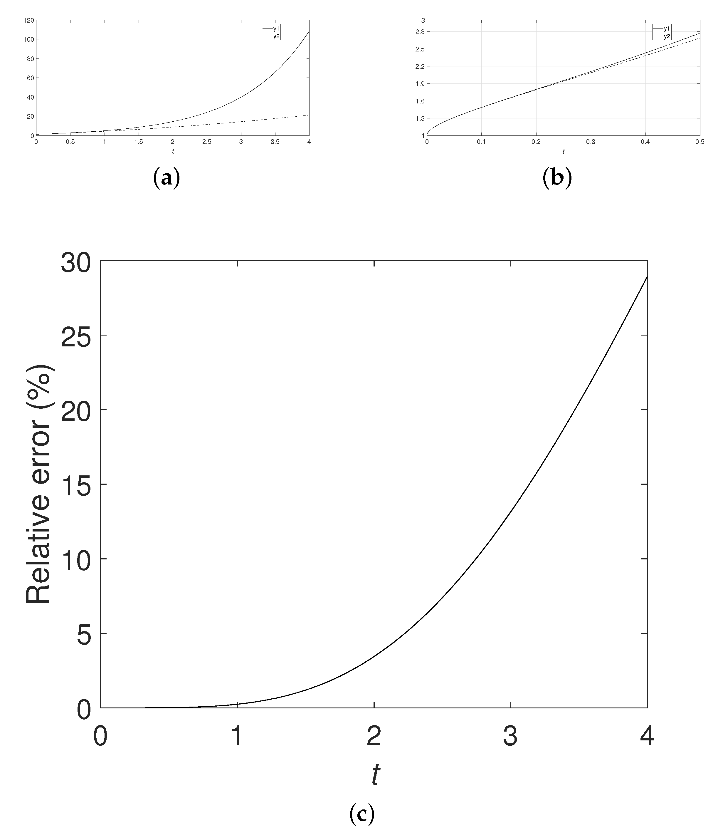
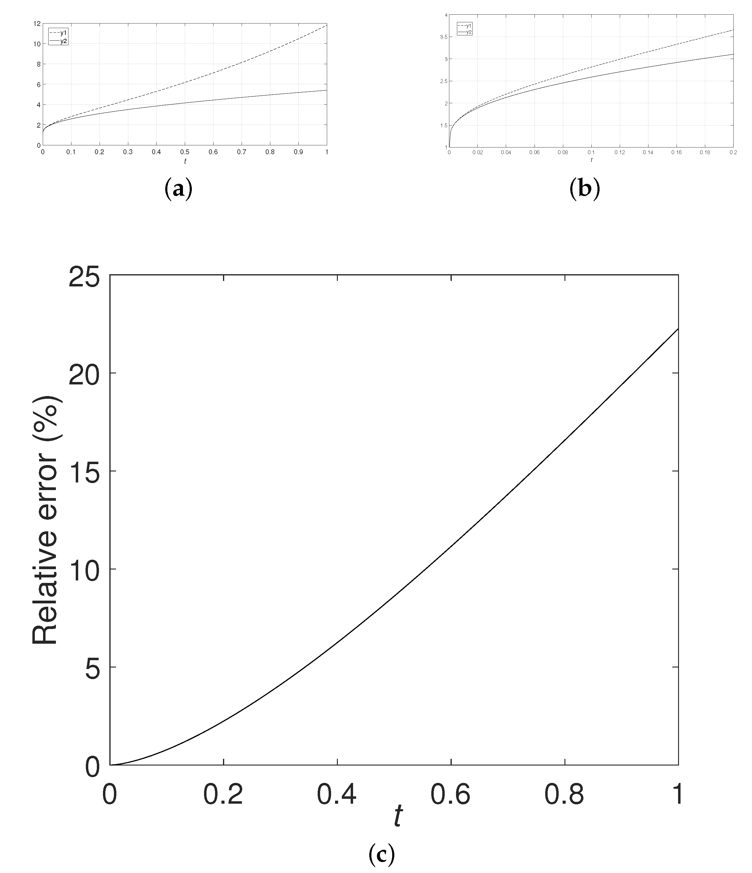
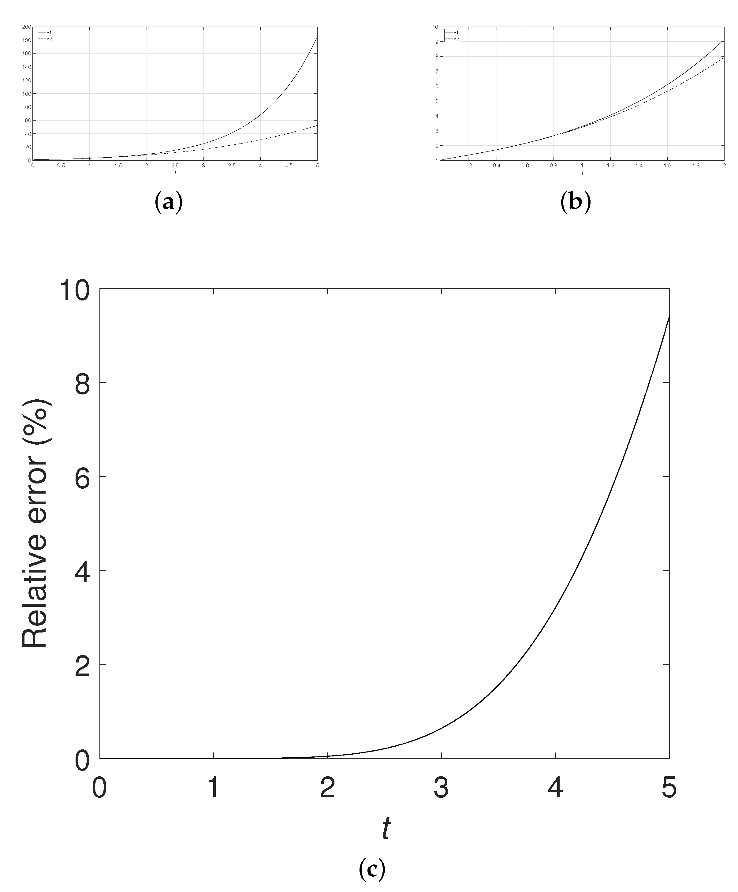
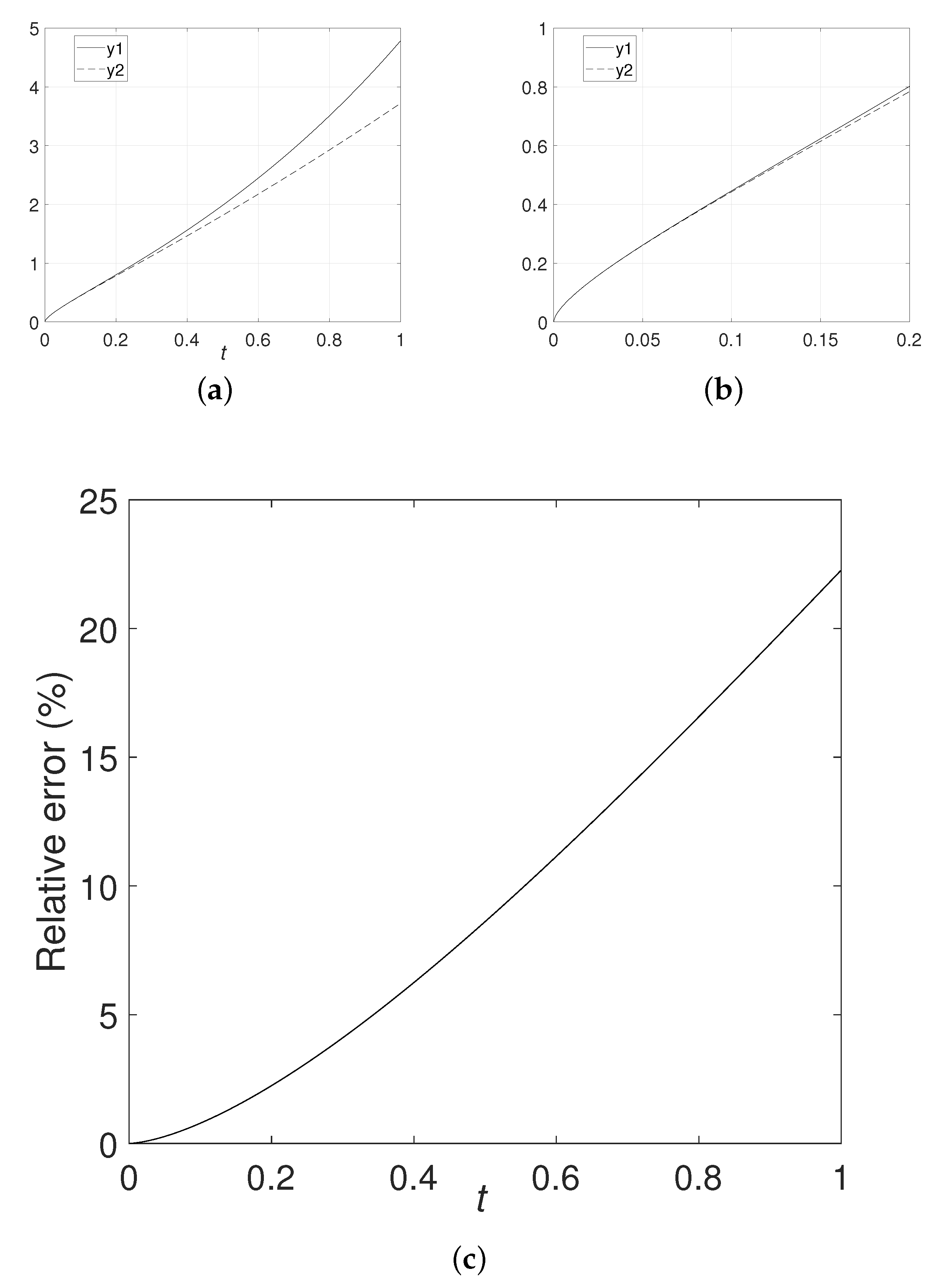
and take numerical simulation. The numerical simulation results are shown in Figure 1 with

ϵ = 0.5

, Figure 2 with

ϵ = 0.2

and Figure 3 with

ϵ = 0.8

. Numerical simulations show that the absolute error and the relative error have high accuracy within a time range, but quickly diverge and may mislead over this time range.

Example 2.

Suppose

ς (t) = \sum_{k = 0}^{\infty} \frac{t^{2 k ϵ + 1}}{Γ (1 + 2 k ϵ)}

. Then, the n order approximate expansion is expressed as

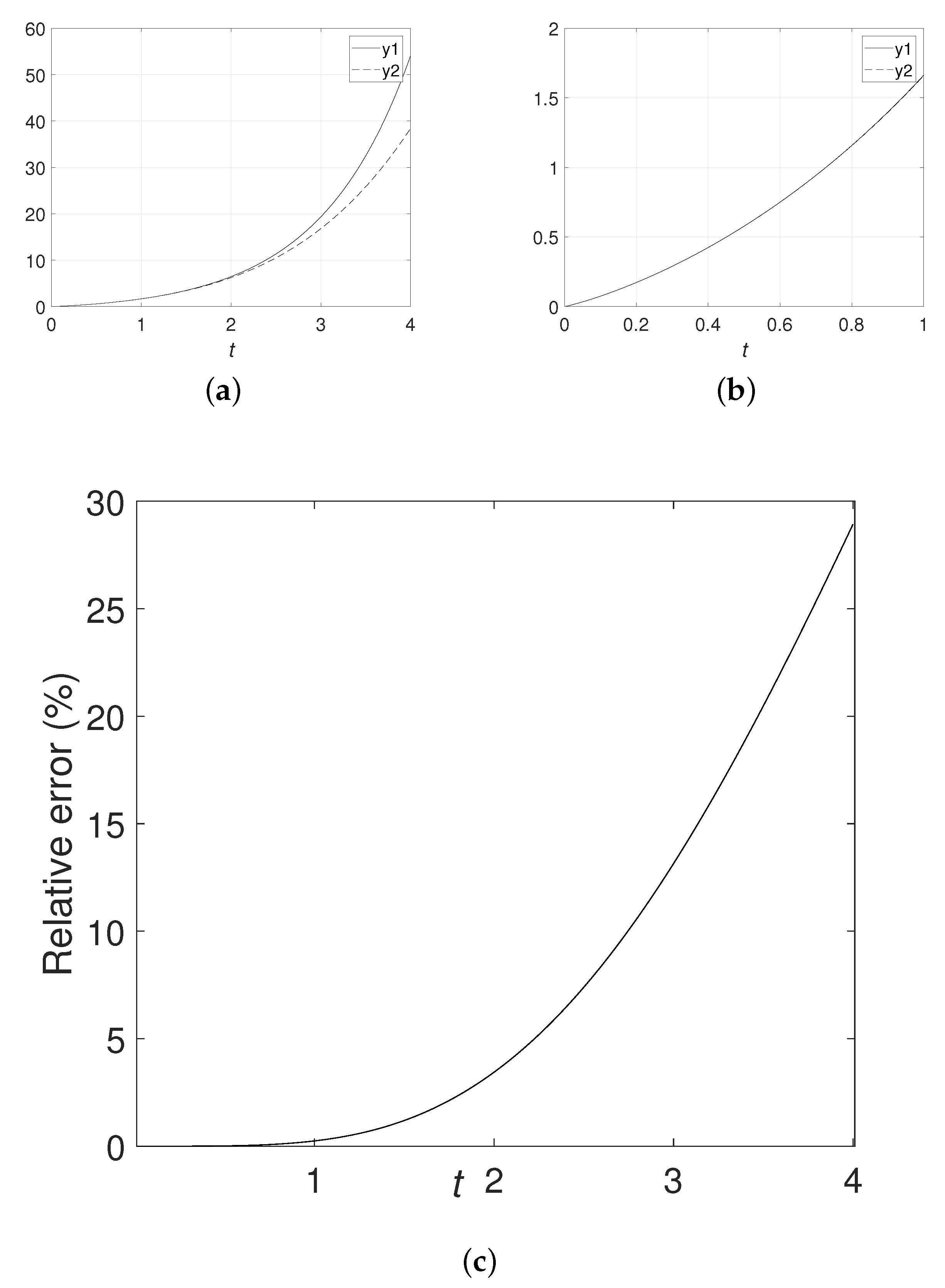
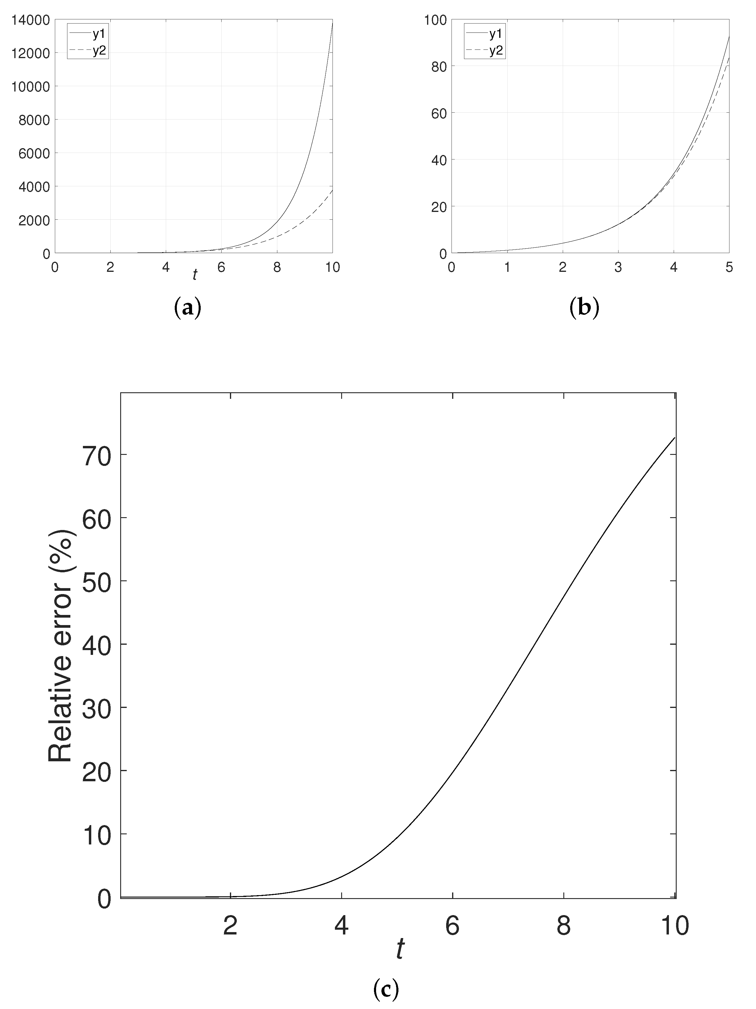
\begin{matrix} {\tilde{ς}}_{n} (t) = \sum_{k = 0}^{n} \frac{t^{2 k ϵ + 1}}{Γ (1 + 2 k ϵ)} \end{matrix}

(37)

Similarly, let

y_{1} = ς (t)

y_{2} = {\tilde{ς}}_{n} (t)

where

n = 4

and take numerical simulation. The numerical simulation results are shown in Figure 4 with

ϵ = 0.5

, Figure 5 with

ϵ = 0.2

and Figure 6 with

ϵ = 0.8

. Numerical simulations also show that the absolute error and the relative error have high accuracy within a certain time range, but quickly diverge and may mislead over this time range.

The numerical simulations in the above examples all verify our theorem analysis. The mentioned method can only be applied in a time range. Over this range, it may mislead.

6. Conclusions

In this paper, we present the detailed analysis process of the fractional reduced differential transform method. Theorem analysis and numerical simulation show that this method can only be applied in a certain time range. Then, by this method, we first need to know the time range. The mentioned can only be studied in this time range. During this time range, the achievement obtained may be mislead.

Data Availability Statement

The datasets analyzed during the current study are available from the corresponding author on reasonable request.

Acknowledgments

This work was supported by The National Natural Science Foundation of China under Grant Nos. 61304062.

Conflicts of Interest

The authors declare that they have no conflicts of interest.

References

Zhao, L. Comments on “Finite-Time Control of Uncertain Fractional-Order Positive Impulsive Switched Systems with Mode-Dependent Average Dwell Time”. CIRCUITS SYSTEMS AND SIGNAL PROCESSING 2020, 39, 6394–6397. [Google Scholar] [CrossRef]
Zhao, L. A note on “Cluster synchronization of fractional-order directed networks via intermittent pinning control”. PHYSICA A-STATISTICAL MECHANICS AND ITS APPLICATIONS 2021, 561. [Google Scholar] [CrossRef]
Shan, W.; Wang, Y.; Tang, W. Fractional Order Internal Model PID Control for Pulp Batch Cooking Process. JOURNAL OF CHEMICAL ENGINEERING OF JAPAN 2023, 56. [Google Scholar] [CrossRef]
Bishehniasar, M.; Salahshour, S.; Ahmadian, A.; Ismail, F.; Baleanu, D. An Accurate Approximate-Analytical Technique for Solving Time-Fractional Partial Differential Equations. COMPLEXITY 2017. [Google Scholar] [CrossRef]
Abdollahi, R.; Khastan, A.; Nieto, J.J.; Rodriguez-Lopez, R. On the linear fuzzy model associated with Caputo-Fabrizio operator. BOUNDARY VALUE PROBLEMS 2018. [Google Scholar] [CrossRef]
Zhao, L. A note on “Cluster synchronization of fractional-order directed networks via intermittent pinning control”. PHYSICA A-STATISTICAL MECHANICS AND ITS APPLICATIONS 2021, 561. [Google Scholar] [CrossRef]
Alam Khan, N.; Abdul Razzaq, O.; Riaz, F.; Ahmadian, A.; Senu, N. Dynamics of fractional order nonlinear system: A realistic perception with neutrosophic fuzzy number and Allee effect. Journal of Advanced Research 2021, 32, 109–118. [Google Scholar] [CrossRef]
Ahmadian, A.; Salahshour, S.; Ali-Akbari, M.; Ismail, F.; Baleanu, D. A novel approach to approximate fractional derivative with uncertain conditions. CHAOS SOLITONS & FRACTALS 2017, 104, 68–76. [Google Scholar] [CrossRef]
Singh, S.; Ray, S.S. Higher-order approximate solutions of fractional stochastic point kinetics equations in nuclear reactor dynamics. NUCLEAR SCIENCE AND TECHNIQUES 2019, 30. [Google Scholar] [CrossRef]
Bohaienko, V.; Bulavatsky, V. Simplified Mathematical Model for the Description of Anomalous Migration of Soluble Substances in Vertical Filtration Flow. Fractal and Fractional 2020, 4. [Google Scholar] [CrossRef]
Salama, F.M.; Hamid, N.N.A.; Ali, N.H.M.; Ali, U. An efficient modified hybrid explicit group iterative method for the time-fractional diffusion equation in two space dimensions. AIMS Mathematics 2022, 7, 2370–2392. [Google Scholar] [CrossRef]
Jaradat, I.; Alquran, M.; Yousef, F.; Momani, S.; Baleanu, D. On (2+1)-dimensional physical models endowed with decoupled spatial and temporal memory indices^★. EUROPEAN PHYSICAL JOURNAL PLUS 2019, 134. [Google Scholar] [CrossRef]
Mukhtar, S.; Abuasad, S.; Hashim, I.; Abdul Karim, S.A. Effective Method for Solving Different Types of Nonlinear Fractional Burgers’ Equations. MATHEMATICS 2020, 8. [Google Scholar] [CrossRef]
Liu, J.G.; Yang, X.J.; Feng, Y.Y.; Cui, P. On the (N+1)-dimensional local fractional reduced differential transform method and its applications. MATHEMATICAL METHODS IN THE APPLIED SCIENCES 2020, 43, 8856–8866. [Google Scholar] [CrossRef]
Ali, G.; Ahmad, I.; Shah, K.; Abdeljawad, T. Iterative Analysis of Nonlinear BBM Equations under Nonsingular Fractional Order Derivative. ADVANCES IN MATHEMATICAL PHYSICS 2020, 2020. [Google Scholar] [CrossRef]
Zhao, L.; Chen, Y. Comments on “a novel approach to approximate fractional derivative with uncertain conditions”. CHAOS SOLITONS & FRACTALS 2022, 154. [Google Scholar] [CrossRef]
Zada, L.; Aziz, I. Numerical solution of fractional partial differential equations via Haar wavelet. NUMERICAL METHODS FOR PARTIAL DIFFERENTIAL EQUATIONS 2022, 38, 222–242. [Google Scholar] [CrossRef]
Arshad, M.; Lu, D.; Wang, J. (N+1)-dimensional fractional reduced differential transform method for fractional order partial differential equations. COMMUNICATIONS IN NONLINEAR SCIENCE AND NUMERICAL SIMULATION 2017, 48, 509–519. [Google Scholar] [CrossRef]
Yu, J.; Jing, J.; Sun, Y.; Wu, S. (<i>n</i>+1)-Dimensional reduced differential transform method for solving partial differential equations’. APPLIED MATHEMATICS AND COMPUTATION 2016, 273, 697–705. [Google Scholar] [CrossRef]
Abuasad, S.; Alshammari, S.; Al-rabtah, A.; Hashim, I. Solving a Higher-Dimensional Time-Fractional Diffusion Equation via the Fractional Reduced Differential Transform Method. FRACTAL AND FRACTIONAL 2021, 5. [Google Scholar] [CrossRef]
Owyed, S.; Abdou, M.A.; Abdel-Aty, A.H.; Alharbi, W.; Nekhili, R. Numerical and approximate solutions for coupled time fractional nonlinear evolutions equations via reduced differential transform method. CHAOS SOLITONS & FRACTALS 2020, 131. [Google Scholar] [CrossRef]
Maisuria, M.A.; Tandel, P.V.; Patel, T. Solution of Two-Dimensional Solute Transport Model for Heterogeneous Porous Medium Using Fractional Reduced Differential Transform Method. AXIOMS 2023, 12. [Google Scholar] [CrossRef]
Mahdy, A.M.S.; Gepreel, K.A.; Lotfy, K.; El-Bary, A. Reduced differential transform and Sumudu transform methods for solving fractional financial models of awareness. APPLIED MATHEMATICS-A JOURNAL OF CHINESE UNIVERSITIES SERIES B 2023, 38, 338–356. [Google Scholar] [CrossRef]
Al-rabtah, A.; Abuasad, S. Effective Modified Fractional Reduced Differential Transform Method for Solving Multi-Term Time-Fractional Wave-Diffusion Equations. SYMMETRY-BASEL 2023, 15. [Google Scholar] [CrossRef]

Figure 1. The absolute error (Figure (a) and Figure(b)) and relative error (Figure(c)) in Example 1 with

ϵ = 0.5

Figure 1. The absolute error (Figure (a) and Figure(b)) and relative error (Figure(c)) in Example 1 with

ϵ = 0.5

Figure 2. The absolute error (Figure (a) and Figure(b)) and relative error (Figure(c)) in Example 1 with

ϵ = 0.2

Figure 2. The absolute error (Figure (a) and Figure(b)) and relative error (Figure(c)) in Example 1 with

ϵ = 0.2

Figure 3. The absolute error (Figure (a) and Figure(b)) and relative error (Figure(c)) in Example 1 with

ϵ = 0.8

Figure 3. The absolute error (Figure (a) and Figure(b)) and relative error (Figure(c)) in Example 1 with

ϵ = 0.8

Figure 4. The absolute error (Figure (a) and Figure(b)) and relative error (Figure(c)) in Example 2 with

ϵ = 0.5

Figure 4. The absolute error (Figure (a) and Figure(b)) and relative error (Figure(c)) in Example 2 with

ϵ = 0.5

Figure 5. The absolute error (Figure (a) and Figure(b)) and relative error (Figure(c)) in Example 2 with

ϵ = 0.2

Figure 5. The absolute error (Figure (a) and Figure(b)) and relative error (Figure(c)) in Example 2 with

ϵ = 0.2

Figure 6. The absolute error (Figure (a) and Figure(b)) and relative error (Figure(c)) in Example 2 with

ϵ = 0.8

Figure 6. The absolute error (Figure (a) and Figure(b)) and relative error (Figure(c)) in Example 2 with

ϵ = 0.8

Disclaimer/Publisher’s Note: The statements, opinions and data contained in all publications are solely those of the individual author(s) and contributor(s) and not of MDPI and/or the editor(s). MDPI and/or the editor(s) disclaim responsibility for any injury to people or property resulting from any ideas, methods, instructions or products referred to in the content.

© 2024 by the authors. Licensee MDPI, Basel, Switzerland. This article is an open access article distributed under the terms and conditions of the Creative Commons Attribution (CC BY) license (http://creativecommons.org/licenses/by/4.0/).

Copyright: This open access article is published under a Creative Commons CC BY 4.0 license, which permit the free download, distribution, and reuse, provided that the author and preprint are cited in any reuse.

MDPI Initiatives

Important Links

Choose an area of interest and we will send you notifications of new preprints at your preferred frequency.

Disclaimer

Analyzing the Approximate Error and the Applicable Condition of Fractional Reduced Differential Transform Method

Abstract

1. Introduction

2. The Definitions and Some Properties of Fractional Calculus

3. Fractional Reduced Differential Transform Method

4. Analyzing the Approximate Error and the Applicable Condition

5. Examples

6. Conclusions

Data Availability Statement

Acknowledgments

Conflicts of Interest

References

MDPI Initiatives

Important Links

Subscribe