Submitted:
17 May 2024
Posted:
20 May 2024
You are already at the latest version
Abstract
Demand flexibility plays a crucial role in mitigating the intermittency of renewable power sources. This paper focuses on an active distribution grid that incorporates flexible heat and electric demands, specifically Heat Pumps (HPs) and Electric Vehicles (EVs). Additionally, it addresses Photovoltaic (PV) power generation facilities and electrical batteries to enhance demand flexibility. To exploit demand flexibility from both heat and electric demand, along with the integration of PVs and batteries, Control and Communication Mechanisms (CCMs) are formulated. These CCMs integrate demand flexibility into the distribution grids to get economic benefits for private households and at the same time facilitate voltage control. Concerning EVs, the paper discusses voltage-based droop control, scheduled charging, priority charging, and up-/down-power regulation to optimize the charging and discharging operations. For heat demands, the on-off operation of the HPs integrated with Phase Change Material (PCM) storage is optimized to unlock heat-to-power flexibility. The HP controllers aim to ensure as much self-consumption as possible and provide voltage support for the distribution grid while ensuring the thermal comfort of residents. Finally, the developed CCMs are implemented on a small and representative community of active distribution grid with 8 houses using Power Factory software and DigSILENT Simulation Language (DSL). This scalable size of the active distribution network facilitates to carefully study symbiotic interaction among the flexible load, generation, and different houses thoroughly. The simulation results confirm that the integration of flexible demands into the grid using the designed CCMs results in the grid benefiting from stabilized voltage control, especially during peak demand hours.
Keywords:
active distribution grid
; battery
; CCM
; electric vehicle
; flexibility
; heat pump
; voltage
1. Introduction
1.1. Motivation and Problem Description
While environmental concerns about global warming intensify, there is a simultaneous and growing demand for energy, particularly in the electrical sector. To supply the growing need for electricity demand with zero emissions, renewable energies are a practical solution. What matters in renewable power generation is the power intermittency. Indeed, the intermittent nature of renewable energies, such as wind and solar power, complicates power dispatch. To overcome this problem, demand flexibility is a workable solution. Demand flexibility can be unleashed in response to renewable power availability on the supply side. The aggregation of demand flexibility needs to be coordinated; otherwise, segregated demand flexibility may not align with the requirements of the power system. Control mechanisms are required to coordinate the flexibility management systems with the power system needs. This is the main idea behind this study to unlock the flexibility potentials of both power and heat demands, including Heat Pumps (HPs), Electric Vehicles (EVs), and batteries, in the presence of Photovoltaic (PV) generation plants. To achieve these aims, this paper designs control mechanisms for the HP, EVs, and batteries. The on-off operation of the HPs coupled with Phase Change Material (PCM) storage is optimized to offer voltage support for the distribution grid by unleashing heat-to-power flexibility. The temperature and mass level of the heat storage are monitored continuously to ensure the residents’ thermal comfort. Regarding the EVs, the charging and discharging operations are optimized by a set of Control and Communication Mechanisms (CCMs) including voltage-based droop control, priority charging, and power regulation. In this way, the preferred State of Charge (SOC) of the EV owners, and Depth of Discharge (DOD) are the main constraints. For PV panels connected to the Battery Energy Storage System (PV-BESS), the CCM establishes the optimal charging and discharging schedule for the batteries to ensure as much self-consumption as possible, while also determining the schedule with the aim of either storing the solar power or releasing it to the grid, in accordance with the flexibility requirements of the power system. Ultimately, the flexible demands are integrated into a 0.4 kV active distribution grid. This integration serves to provide voltage support for the network while simultaneously addressing the thermal comfort requirements for heat demands and fulfilling the driving needs of EV owners.
1.2. Literature Review
In the literature, there are many studies discussing the flexibility potentials of power and heat demands in different sectors, including residential [1], industrial [2], agricultural [3], and commercial [4] sectors. In urban areas, the residential sector is the main source of demand flexibility [5]. In households, EVs, HPs, electrical batteries, and roof-top PV panels can provide flexibility for distribution grids. To enhance the effectiveness of energy flexibility within the power system, it is crucial to first coordinate and subsequently integrate the energy flexibility measures into the overall power system. In other words, the segregated energy flexibility may not meet the power system’s needs. To facilitate coordination among the flexibility potentials of various demands, it is essential to implement control and coordination schemes. Control schemes enable the optimization of processes such as charging/discharging of EVs on the demand side, aligning it with the availability of renewable power on the supply side. Without such coordination, demand flexibility might be activated during periods of excess renewable power or when electricity prices are low.
By retiring fossil fuel vehicles, the share of EVs is increasing considerably. From an environmental point of view, it limits global warming by the reduction in greenhouse gas emissions [6]. Initially, this surge in EVs might pose challenges to power grids, especially in the context of supplying a large number of new mobile electric demands, potentially posing a threat to weaker power systems, e.g., in the form of power congestion or voltage drop. However, upon closer examination of the flexibility and storage capabilities inherent in EVs, it becomes evident that they can play a pivotal role in facilitating the integration of renewables into power systems [7]. The flexibility potentials of EVs can be discussed in two categories: (1) Private parking lots [8] and (2) Public parking lots [9]. Regarding home parking, the demand flexibility of EVs is harnessed during non-working hours, primarily at night when the EVs are parked [10].
While the EV flexibility is limited by the owner preferences, e.g., arrival/departure SOC and dwelling time, the electrical batteries offer greater flexibility without being affected by human preferences. The batteries can be connected to the grid either independently or in conjunction with a renewable self-generation facility [11]. Among studies in urban areas, Roof-top PV (RPV) sites are one of the most popular micro-self-generation facilities due to zero noise and emission [12]. Similar to batteries, the RPVs can be connected independently to the power grid or integrated with an electrical battery. In the former, the flexibility potentials of the RPVs are restricted to daylight hours. In the latter, the solar power can be stored in the batteries during the day and discharged at nighttime hours either to the household loads or to the grid [13]. A recent study proposed flexibility indices for RPVs in smart homes to enable household controllable appliances to benefit from demand flexibility [14].
In the residential sector, heat pumps’ popularity is increasing due to their high efficiency, i.e., they can generate three to five times as much heat energy as they are using electricity [15]. In many studies, heat pumps are addressed with heat storage, including water tanks [16] and PCM storage [17]. The incorporation of heat storage enhances the flexibility potential of the heating system. It enables drawing power from the grid during periods of low electricity prices or a surplus of renewable energy, effectively unleashing heat-to-power flexibility to offer voltage support [18]. On the electrical side of the heat pumps, the compressor can be turned on/off on short notice in response to flexibility requests from the local system operator [19]. Moreover, for variable-speed compressors, the power consumption can be turned up/down without needing a binary working state of the heat pumps, eliminating the requirement for full stop or full operation [20]. On the thermal side of the heat pump, the time constant of the thermal mass, including building envelopes and indoor air, is longer than the electrical side. It means that the heat pump can swiftly respond to the flexibility needs of the power system without causing a substantial change in the indoor air temperature.
In order to unleash the flexibility potentials of the controllable devices, e.g., HPs, EVs, RPVs, and batteries, aligned with the power system requirements, control mechanisms are required. Control mechanisms make it possible to optimize the operation schedule of power and heat demands to provide as much flexibility as possible to upstream networks. In [21], a model predictive control was addressed to unlock the heat-to-power flexibility of heat pumps; consequently, it showed 20% operation cost savings and 12% energy consumption savings in comparison to conventional PID controls. In [22], a droop charging control was proposed for EVs contributing to the frequency regulation of distribution grids with high penetration of renewables. In [23], a rule-based algorithm was suggested for peak shaving control in commercial buildings utilizing coupled PV-battery systems. In addition, other control methods were highlighted in recent literature to control and manage components of distribution grids and microgrids as combined master-slave and droop control [24], adaptive droop control based on the fuzzy algorithm [25] and virtual resistance damp control [26].
Distribution grids derive diverse benefits from demand flexibility, including voltage support [27], frequency regulation [28], congestion management [29], peak-shaving and valley-filling [30], enhancing grid resiliency and stability [31], loss reduction [32], emission reduction [33], and cost efficiency [34]. A recent study was conducted to assess the flexibility potentials of a carbon-neutral German energy system [35]. The results underlined that electrical mobility and heat sectors not only facilitate carbon-neutral energy systems but also enhance the flexibility of the energy systems. In this context, it is necessary to explore the flexibility potentials of multi-carrier energy systems and Power-to-X systems, which are anticipated to expand further in the near future.
1.3. Paper Contributions and Organization
This paper proposes an active distribution grid that is comprised of flexible heat pumps with thermal storage, EVs, electrical batteries, and PV generation facilities. The problem aims to control the operation of the flexible heat and electric demands to offer voltage support for the distribution grid. Therefore, CCMs are addressed to unlock the flexibility potentials in response to the power system’s requirements. To sum up, the main contributions of this paper can be summarized as follows:
- (1)
- Designing comprehensive CCMs for power and heat demands, i.e., EVs, HPs, and PV-BSS, to unlock the power and heat-to-power flexibility potentials in alignment with power system requirements and consumer preferences, and economic benefits.
- (2)
- Offering voltage support for the active distribution grid by leveraging demand flexibility derived from power and heat demands.
- (3)
- Justifying integration of CCMs along with flexible power and heat demands into the active distribution network using Power Factory software and DSL.
The rest of the paper is organized as follows. Section 2 represents the mathematical formulations of EVs, HPs, PV, and BESS and the structures of the associated CCMs. Section 3 describes the input data and simulation results in Section 3.1 and Section 3.2, respectively. Finally, Section 4 concludes the study.
2. Problem Formulation for Operation and Control of Flexible Demands
In this section, the structure of CCMs is explained, accompanied by mathematical formulations for the flexible power and heat demands. The CCMs and mathematical models are stated for EVs, HPs, and PV-BESS individually.
Two-level control approach is implemented to address both the forecasting error and communication failures in the scheduling device operations, including HP, EV, and BESS to meet users’ requirements. Figure 1 illustrates the decentralized control and operation of flexible loads within an integrated energy system, employing the bi-level control as follows:
(1) First Level: Involves signaling and re-coordination as a response to issues
(2) Second level: Focuses on local translation planning and the control signals implementation
At the first control level, the estimation of device operations is conducted by considering forecasted demand, and electricity spot price information, users’ preferences, status of energy storage, and formulating operation schedules. The operating schedule is subject to re-scheduling to compensate for forecasting errors in demand. This control level needs online communication with the control server regularly via the Internet.
The second level of control have the capability to override the command from the first-level control based on the upper and lower limits of the state of energy available in the storage devices as well as the node voltage condition at the Point of Coupling (POC) of controlled devices. Since the state of charge of energy storage and node voltages are measured locally, there is no need for internet communication. Hence, the error in the operation schedule is compensated while also supporting local node voltage regulation where applicable.
2.1. Electric Vehicles
In this part, CCMs are designed for EVs to offer voltage regulation for the supply side and meet the EV owners’ preferences, e.g., SOC and DOD, on the demand side. Therefore, three different control schemes are suggested to optimize the charging and discharging of the EVs as follows:
- (1)
- Scheduled charging
- (2)
- Up-/down-regulation
- (3)
- Priority charging
Note that if none of these schemes are selected by EV owners, the EV will charge at the rated power of the charger until it is fully charged or disconnected.
Figure 2 illustrates the comprehensive control flowchart depicting the three control mechanisms for the EV operation. In the following, the structure of the control mechanisms is described qualitatively and formulated mathematically.
Moreover, Figure 3 describes the structure of EV charging control encompassing voltage at POC and transformer loading. This figure explains how the three control mechanisms contribute to the high, middle, and no flexibility based on the voltage magnitude and transformer loading. When the voltage at POC falls within the range of 0.98 to 1 p.u, there is high flexibility in the network. In such cases, scheduled and priority charging are chosen. Note that demand flexibility remains essential for the power grid even when nodal voltage is normal. This is because demand flexibility plays a crucial role in maintaining grid stability by adapting to real-time variations in electricity consumption. With a decrease in voltage magnitude to the range of 0.98 to 0.92, medium flexibility is available in the network, leading to the selection of droop control and priority charging. Lastly, when the voltage magnitude drops below 0.92, indicating a lack of flexibility in the network, priority charging becomes the only available charging option.
To initiate the modeling of the CCMs, let us denote as the state of charge of the EV battery at a given time t, then the EV availability is defined as the binary variable . is equal to 1 if the EV is connected physically to the charger and takes 0 otherwise. The binary variable states the EV battery status, if the EV is connected to the charger and the battery is not fully charged, takes the value of 1 and takes 0 otherwise. Therefore, S(t) can be formulated as follows:
The designated control mechanism ensures that the EV owners have the minimum preferred SOC level, , at the time of departure. Therefore, the minimum required state of the EV battery, is defined as follows:
After the introduction of primary variables, the fundamentals of the three control mechanisms are explained in the next subsections.
2.1.1. Droop Control
The droop control provides voltage regulation by unlocking the flexibility of EVs connected to buses in the radial structure of distribution networks. Droop control is an integral part of all the three control methodologies defined earlier. Based on the user’s preferences, these control schemes are anticipated with or without the support of droop control. To formulate the droop control mechanism, it is supposed that VPOC(t) and Iline(t) represent the voltage at the POC of EV and line current, respectively and Preg(t) is the regulation power by EVs. It is worth mentioning that different flexible demands have diverse response characteristics to voltage and frequency variations; therefore, variable droop coefficients ensure optimized coordination of flexible demands in response to some deviations in power grids. Then, the droop coefficients are calculated as follows:
As the node voltages along the radial feeder is different, so will be the droop coefficient. The lower limit for the voltage droop coefficient is determined at 0.92 p.u, so that there is no EV being charged, unless in priority condition discussed later, and the terminal voltage may remain above 0.9 p.u with some margin for increase in other loads. The upper limit of 0.98 p.u is assumed considering that the load at the far end of the feeder can be operated with rated capacity at this voltage level. In Eq. (3), the voltage coefficient of droop control Kv(t) is calculated based on VPOC(t) to provide up-/down-regulation for the VPOC(t). Similarly, according to Eq. (4), current coefficient of droop control Kl(t) is chosen to manage line loading within the critical limit icrit and the full loading of the connected bus. Finally, the droop control coefficient k(t) is determined as the minimum value between kv(t) and kl(t) according to the following expression:
where the parameter Cdroop indicates the EV owner’s preference to participate in droop control, in which it takes value 1 for the participation and takes 0 otherwise. Figure 4 illustrates the droop control procedure for the voltage and current coefficients.
2.1.2. Scheduled Charging
In this control mechanism, the EV owners are allowed to select an option to participate in scheduled EV charging. Therefore, the binary variable Csch is defined to state the EV preference to participate in the scheduled charging, in which it takes 1 in the case of participation and 0 otherwise. The scheduled power Psch(t) is generated either through cloud computing, utilizing an optimal solution for power regulation in the grid in real-time, or it is determined by an online or app-based optimal solution defined by the user and stored in the controller for offline use. In case the user is not willing to contribute to the scheduled charging program, the EV will start charging immediately with rated power of the charger Prated. To distinguish between the selection of droop control and scheduled charging, two variables as flexible power and flexible control signal Cflex are defined as follows:
determines the flexible power required for charging EV, which can be based on rated or scheduled charging power as well as droop coefficient, whereas represents the logical crieria for selection of charging power value of .
2.1.3. Up- and Down-Regulation
In power systems with high renewable power penetration, the power system may face deficit/excess of renewable power. To counterbalance the intermittent power, EVs can utilize their flexibility to discharge/charge to/from the power grid, thereby offering down-/up-regulation in the opposite direction of power system imbalance.
To formulate the regulation scheme, consider Creg as the binary variable denoting the EVs’ inclination to participate in power regulation program, and Pv2g(t) as the power interchange between EVs and the grid. To participate in the power exchange, SOC(t) must be between 20% and 100%. This constraint ensures that EV battery is not discharged below 20% when EV is supplying regulated power to grid. Then, consider the control signal for up- and down-regulation as Sup(t) and Sdn(t), respectively; control signal for power regulation as Sreg(t) and the regulation power as Preg(t). Therefore, the control conditions can be formulated as follows:
Note that the regulation power Preg(t) is calculated by the power system operator. Defining the activation of the Vehicle-to-Grid (V2G) signal as Cv2g(t), we can express this as:
Equation (11) determines activation of power regulation Cv2g(t) based on user preference Creg and power regulation requirement Preg(t). When the power regulation signal is active, power interchange Pv2g(t) is initiated according to equation (12). When the EV is fully charged during down regulation or discharged down to 20% during up regulation, then the power regulation signal Cv2g (t) is activated to stop charging/discharging of the EV.
2.1.4. Priority Charging
As previously stated, the control mechanism of EVs must align with the preferences of the EV owners at the departure time. To ensure the attainment of the minimum SOC at the departure time, the controller generates a priority signal Cpriority(t). This signal is derived from the state of charge information, SOC(t), and the user-defined minimum required , at the estimated time of departure. Hence, the formulations for the total time required for minimum SOC charging and the remaining time until departure can be expressed as follows:
The controller logic is structured to activate the priority signal when the charging time of the EV to reach the minimum SOC level is less than 15 minutes before the estimated departure time. Upon activation of the priority signal, the EV undergoes charging to reach the minimum SOC level using the rated power, and subsequently, droop control is employed until the vehicle is either fully charged or disconnected. During this period, the EV is precluded from participating in grid regulation to ensure readiness for departure. The mathematical expression for this logic can be represented as follows:
2.1.5. Charging Power
Finally, the general charging power of EV for the all control mechanisms, Pchar(t), is computed based on the participation of EVs in the three control mechanisms, including scheduled charging, up-/down-regulation and priority charging, as follows:
This expression indicates that the priority charging is active when the priority signal is active, regulation charging is active when the V2G signal is active, and the scheduled charging is active when both the priority and V2G signals are inactive.
2.2. Electric Batteries and PVs
Electrical batteries offer power flexibility for the distribution grid in two directions: as a source of demand, i.e., charging from the grid, and a supplier, i.e., discharging to the grid. In this study, the batteries are connected to the PV arrays. Therefore, when electricity prices are high, both the electrical batteries and PV panels inject power into the distribution grids. In this scenario, the PV-BESS supplies local demands and discharges the remaining capacity to the distribution grids to optimize self-consumption. Conversely, during periods of low electricity prices or excess renewable power generation, the batteries are charged by both PV generation and power drawn from the distribution grid. Figure 5 depicts the flowchart of designed CCMs for the PV-BESS to unlock the battery flexibility in response to requirements of the distribution grid.
The Battery Management System (BMS) determines the charging and discharging scheduling of the PV-BESS. Assume as the state of the charge of battery at a given time t, and and as minimum and maximum SOC levels of the battery, respectively. To limit the cycling and avoid haunting effect of battery switching in upper and lower thresholds of the SOC boundary, a dead zone is considered as 10% and 20% for the and , respectively. Therefore, the discharge schedule is further suspended until the is greater than +20%. Similarly, the charging of battery is stopped once battery reaches and further charging is suspended until the is less than -10%. Accordingly, the control logic of the PV-BESS is formulated in the following subsections.
2.2.1. Fully Charged Condition
When the SOC of the battery is attaining 100%, further charging is disabled until the battery is discharged to level (). This logic is called charging condition CC1(t) or fully charged condition and can be formulated as follows:
2.2.2. Peak Shaving Mode
Peak Shaving (PS) is a function incorporated within the BESS to mitigate peak loads on the distribution grid during periods of peak demand. When the PS mode is activated by the BMS, i.e., PS=1, charging of BESS is disabled during the peak hour period, e.g., hours 17-20. The PS mode is called charging condition CC2(t) and is formulated as follows:
Considering charging conditions CC1(t) and CC2(t), the general charging condition of the battery CC(t) is satisfied when charging conditions 1 and 2 are fulfilled as follows:
2.2.3. Fully Discharged Condition
Battery storage is considered fully discharged when the SOC is 20% or below. This SOC level is considered as . The battery is not able to discharge beyond this SOC level. The discharge plan is further suspended until the is greater than +20% to avoid hunting as mentioned. This control logic is called discharging condition DC1(t) and is formulated as follows:
2.2.4. Power Export Mode
Power Export (PE) mode is a function incorporated within the BESS to sell power to the distribution grid. When the PE mode is activated by the BMS, i.e., PE=1, the battery discharge to the distribution grid. When the PE mode is disabled, i.e., PE=0, the BMS restricts power discharge from the battery and prohibits the sale of power to the grid from the battery storage. In this operation mode, the BMS is constantly monitoring the power at the main meter and power generation from the solar panels PVgen(t). When the power exported to the grid is greater than PV power generation, the battery storage reduces the discharged power. This makes it possible to sell PV power generation to the distribution grid during high electricity price, or during deficit of renewable power generation, and use battery storage to supply local residential demands. The logical control of the PE mode is formulated as follows:
Note that the PE mode is represented as the discharging condition DC2(t).
2.2.5. Charging and Discharging Power
Henceforth, the charging and discharging power of the batteries can be stated based on the abovementioned control logics. The charging power of the battery is formulated as follows:
In Equation (23), the charging power is determined by the BMS and is limited to the rated charging power of the inverter , which supplies the DC power of the battery by grid connection. Note that the variable denotes the available battery power at time given t, regardless of the charging condition. In the similar way, the BMS determines the discharging power using the following formulation:
where denotes the battery discharging power, is the available battery discharging power, and is the power interchange between the battery and the distribution grid.
2.3. Thermal Devices
In this study, besides addressing power demands, heat demands are modeled. This is done to leverage heat-to-power flexibility for providing voltage support. In this section, the control logic as well as the mathematical formulations of the thermal devices, including HP and PCM storage, are stated.
Figure 6 illustrates how a HP can enhance grid voltage regulation at the POC while meeting thermal demand. If the terminal voltage at POC decreases from 1 p.u to 0.95 p.u, the HP operates according to its regular schedule, offering flexible operation. If drops below 0.95 p.u, the HP is deactivated until the voltage recovers to 0.98 p.u or the thermal storage reaches a critical reserve condition to meet additional demand. However, user priority enables the HP to operate regardless of conditions. To have a general overview about the CCM for thermal devices, Figure 7 illustrates the flowchart of the presented CCM for the heating system.
2.3.1. Heat Pump
In general, heat pumps produce 3-5 times more heat energy than the electricity they consume. The thermal power delivered by the heat pump as well as the inflow/outflow temperatures can be stated as follows:
where is flow rate of Heat Transfer Fluid (HTF) through HP for thermal power delivery, is the rate of heat energy delivered by HP, is the coefficient of performance of HP, is the electrical power consumed by the HP compressor, denotes the outflow temperature of the HTF, and is the inflow temperature of the HTF into the heat exchanger.
2.3.2. Heat Storage
Phase change material and Latent Thermal Storage (LTS) offer certain advantages over sensible heat storage, e.g., water tanks. High energy density, constant temperature during phase change and compact storage design are the most important advantages in comparison to the sensible storage ones. The PCM stores thermal energy without significant change in the storage material. The energy stored in a PCM due to a temperature increase from T1 to T2 can be determined as follows [36]:
where is energy storage capacity of the PCM, is the mass of PCM material, and denote specific heat of PCM in solid and liquid phases, respectively, expresses melting temperature of PCM, and state initial and final temperatures of the PCM material, respectively, is the melt fraction and shows latent heat of fusion of material.
For a comprehensive understanding of the energy flow in the PCM storage, Figure 8 illustrates the energy dynamics in a conceptual PCM storage system.
Based on the figure, the energy balance equation of the PCM can be represented as follows:
where denotes the rate of heat energy stored in tank, shows the rate of heat energy entering storage tank from the source, i.e., the HP, represents the rate of heat energy leaving the tank to the HP, is the rate of heat energy leaving the tank for district heating, indicates the rate of heat energy entering the tank as a return from the district heating, and explains the rate of heat loss to the environment.
3. Numerical Studies
In this section, the numerical studies are described. Firstly, the input data of the test grid are explained. Thereafter, the simulation results are described and discussed.
3.1. Input Data and Test Grid
In order to show the proficiency of the suggested CCMs, a radial distribution network is considered in Figure 9. Based on the figure, the test grid is comprised of 8 EVs, 8 HPs, 8 PV-BESS, 8 household demands and 2 residential areas. These are connected to the external grid through a 2-winding transformer.
The heating system of the households includes a HP and PCM thermal storage. The storage tank has a 500 Liter capacity with a usable storage capacity of 15 kWh. The controllable heat pump can be turned on and off only with a thermal output of 9 kW. The other technical data of the PCM storage and the HP are described in Table 1 and Table 2, respectively. Table 3 represents the complementary data about the EVs, BESS, and PV units.
3.2. Simulation Results and Discussions
In this section, the simulation results of the case studies are discussed. The active distribution grid consist of flexible power and heat demands to provide flexibility services, i.e., voltage regulation. In order to study the impacts of different flexible demands on the distribution grid operation, different case studies are addressed as follows:
Case Study 1: in this state, only the household demands are considered in the network; therefore, the flexible HPs, EVs and PV-batteries are disregarded. This is a base case without demand flexibility.
Case Study 2: in this state, the HPs are integrated to the household demands; as a result, the active distribution grid benefits from the heat-to-power flexibility.
Case Study 3: in this state, the EVs and HPs are integrated to the household demands; then, the network utilizes the power and heat-to-power flexibilities simultaneously. To discuss different charging schemes of EVs, three scenarios are designed for this case study as: (1) Charging priority (2) V2G and droop control (3) V2G, droop control and schedule charging.
Case Study 4: in this state, all the flexible demands, including HPs, EVs, PV-BESS as well as the household demands are integrated to the distribution grid. This is the most complete case study where the active distribution grid takes the advantages of all flexibility potentials.
Figure 10 shows the voltage magnitude at different buses, accumulative power demand of residential areas, power loading of different lines and the transformer loading for case study 1. In this case study, neither flexible demand nor CCMs are addressed. In subfigure (a), the daily demand can be divided into three sections: valley, from hours 1-6; shoulder, from hours 7-16; and peak, from hour 17-24. Despite the difference in the actual demand between the two residential areas, the three demand sections are observed in the transformer loading and line loading in subfigures (c) and (d), respectively.
Although we can observe the three slots for valley, shoulder, and peak in the voltage profile, the valley and peak voltage sections occur during the peak and valley demand slots, respectively. Therefore, when the line loadings are between 20-40% during valley demand, the bus voltage magnitudes vary between 0.96-1 p.u. in the peak period. In contrast, during peak demand, when the line loadings increase up to 80%, the voltage magnitudes drop to approximately 0.92 p.u. Note that this represents the baseline case study, wherein no flexible demands are considered. Upon integrating HPs, EVs, and the PV-BSS into the grid, there is a possibility of voltage magnitude deterioration during peak demand hours. Consequently, CCMs will be implemented in subsequent case studies to provide voltage regulation as additional heat and power demands are introduced to the distribution grid.
Figure 11 describes the operation dynamics of the active distribution network in case study 2 when the HPs and associated CCMs are integrated to the grid. Regarding the PCM temperature in subfigure (a), it is evident that the storage temperature peaks between approximately 50-65°C during nighttime from hours 1 to 6 and remains elevated until hour 9. Subsequently, the storage temperature decreases to 35°C due to low household heat demand when residents are out at work. As time passes and residents return home from the workplace, household demand increases, leading to a gradual rise in storage temperature from hour 14.
During the peak demand period, hours 17-24, which corresponds to the valley of the voltage profile, the temperature of the PCM begins to decrease. This indicates that HPs are extracting heat energy from the storage precisely when there is a high heat demand, and the voltage profile is at its lowest. In this manner, the CCM supplies the HPs with energy from the PCM, effectively contributing to voltage regulation for the grid.
Subfigure (b) illustrates the voltage magnitudes for different buses when the flexible HPs and PCM storages are integrated into the grid through the CCMs. Comparing the voltage profile with subfigure (b) in case study 1, despite the addition of heat demands to the distribution grid, the CCMs effectively maintain the voltage magnitude within the lower and upper permitted thresholds, i.e., 0.92-1.08 p.u. In essence, the CCMs unleash the power-to-heat flexibility of the HPs and utilize the storage capacity of the PCM to regulate the bus voltage magnitude while simultaneously meeting the residents’ heat demand. In this context, we observe greater variations in the voltage profile compared to case study 1. The primary reason for this difference is the on-off switching operation of the HPs.
Regarding line loading in subfigure (d), there is an increase compared to case study 1. Additionally, it displays more fluctuations in the loading profile attributed to the switching operation of the HPs. It’s noteworthy that the step-wise changes in voltage and line loading demonstrate the responsive actions of the CCMs to the switching operations of the HPs in order to regulate bus voltages.
Figure 12 illustrates the operation dynamics of the grid for case study 3 where both the HPs and EVs are integrated into the grid. Subfigure (b) depicts the voltage magnitudes at network buses. The graph reveals two key points. Firstly, with the integration of EVs into the grid, there is an increase in voltage variation. Secondly, during the early nighttime, i.e., hours 1-2, when EVs are connected to the grid for charging, the voltage magnitude remains lower compared to the preceding case where no EVs are involved. Compared to the previous case study, although EVs and HPs are added to the distribution grid as new demands, the CCMs unlocked the heat and power flexibility to offer voltage regulation.
In subfigure (c), illustrating line loading, two noteworthy points should be highlighted. Firstly, the addition of EVs to the network results in an increase in line loading percentage during the valley period. Although there is a noticeable but less pronounced increase in the shoulder and peak periods, the primary escalation occurs during the valley period when most EVs are connected for night charging. Secondly, the line loading profile undergoes more frequent fluctuations due to the charging and discharging schedules of the EVs.
Subfigure (d) explains the SOC of the EV batteries. As depicted in the graph, the majority of charging schedules occur during valley and peak demands, with less charging taking place during the shoulder period. This pattern is attributed to the fact that most EVs are connected to home parking during nighttime, i.e., hours 1-8, and outside of working hours, i.e., 16-24, when residents return home from workplaces.
To elaborate on the various CCMs for EVs, Figure 13, Figure 14 and Figure 15 the grid’s dynamics for three scenarios including (1) charging priority, (2) V2G and droop control, and (3) V2G, droop control, and scheduled charging, respectively.
To distinguish the functionalities of the three scenarios, we focus on the voltage and SOC diagrams of the EVs. It is evident that the strength of voltage control increases from control scenario 1 to 3; therefore, we should anticipate greater voltage control stability in scenario 3 than in scenario 1.
In the first scenario, Figure 15, EVs are charged to 100% throughout all time slots without considering voltage conditions. In this state, the average voltage of the grid is 0.9578 p.u. during the peak period. In the second scenario, as depicted in Figure 16, most EVs reach 100% SOC during valley and shoulder periods. However, some EVs reduce the maximum SOC to 60-80% during the peak period to contribute to voltage regulation on the grid. Consequently, the average voltage magnitude of the grid increases to 0.9593 in the peak period. In the third scenario, based on the SOC diagram of Figure 17, more EVs participate in the voltage regulation program. Here, some EVs not only limit the maximum SOC but also restrict the charging rate to lower values following droop control. This results in an increase in the average voltage to 0.9602 p.u. in the peak period.
As a result, it is evident that the integration of more CCMs into the EV charging control leads to an enhancement in the voltage stability of the distribution grid.
Figure 16 represents the dynamics of the distribution grid for the most comprehensive state, case study 4, incorporating all flexible demands, including HPs, EVs, and PV-BESS, connected to the network.
Subfigure (b) illustrates the voltage profile. According to the graph, upon the integration of the PV-BESS into the grid, the designed CCM strives to stabilize the voltage magnitude during peak hours. This is evident at hour 17 when there is a noticeable increase, up to around 0.98 pu, in the voltage magnitude. Concurrently, there is a decline in the line loading depicted in subfigure (f) at hour 17, indicating that household demands are being supplied by the local PV-BESS.
Subfigure (d) depicts the power generation of the PV system. As evident, solar power generation initiates at around 6 am during daytime hours. The peak of solar power generation is observed in the midday, gradually decreasing to reach zero by hour 20. The solar panels are connected to the BESS, allowing for a decision to either supply the local demands directly on the line or store excess power in the batteries. As illustrated in subfigure (g), the SOC of batteries increases from 20% to 60% from hours 1 to 15, reaching its peak shortly after that for most batteries. This behavior is primarily attributed to the BSS charging from the PV system during the shoulder period and subsequently supplying the local demands during the peak period, specifically from hour 17 onwards.
Subfigure (h) illustrates the power transactions between 8 households and the grid. Positive transaction power values indicate power selling to the grid, while negative values represent power purchasing from the grid. According to the graph, households equipped with flexible heat-power demand and storage have the capability to meet their local demand at certain time slots and also sell excess power to the grid during specific periods. As observed in the diagram, during the valley and shoulder periods, households draw power from the distribution grid. In the peak hours from 17 to 19, households sell power to the grid, providing voltage support. In the remaining peak period from hours 19 to 24, most households minimize power purchases from the distribution grid and meet their demands locally through heat and power storages.
Figure 17 illustrates the secondary controller’s action in correcting errors in the forecasted schedule. This figure is depicted for one EV, i.e., EV2, to clearly describe this matter. The EV was scheduled to depart at hour 10 with a minimum SOC requirement of 80%. Incorrect charging schedule estimation prompted a priority request from the secondary control at hour 4, leading the EV to start charging at the rated power, deviating from the planned power level schedule. Once the EV reaches the minimum required SOC, it continues to charge to 100% using the droop control. Based on the subfigure (c), the red diagram depicts EV’s participation in regulation power, but a regulation cut-off around hour 4 occurs due to the activation of priority charging at midnight.
The primary objective of the presented case studies was to provide voltage support for the grid by unlocking the flexibility of heat and power demand. This was achieved through the design of CCMs. The graphical representation in the presented voltage profile figures demonstrated how the daily voltage profile remains stable in response to the addition of loads, including HPs and EVs. To quantify the voltage stabilization, Table 4 illustrates the average voltage magnitude for the peak period and the entire day. According to the table, despite the integration of additional demands such as EVs, HPs, and batteries into the grid, not only does the bus voltage not decrease, but the CCMs also unleash the flexibility of power and heat demands, enhancing the voltage profile.
4. Conclusions
In this paper, an active distribution network was examined, leveraging the flexibility potentials of both electrical and heat demands to facilitate voltage regulation at the distribution level. The study devised Control and Coordination Mechanisms (CCMs) tailored for flexible demands, encompassing Heat Pumps (HPs), Electric Vehicles (EVs), and Photovoltaic-Battery Storage Systems (PV-BSS), with the aim of unlocking the power and heat-to-power flexibility inherent in these demands.
Concerning the heating system, HPs were linked to Phase Change Material (PCM) storage to augment their inherent flexibility. The PCM facilitated the storage of heating energy during off-peak hours or when there was an excess of solar power availability. The heating system was integrated into the distribution grid using designed CCMs to regulate the on-off operation of the HPs and manage the storage temperature of the PCM in response to the voltage requirements of the distribution network.
Various control mechanisms were explored for EVs to provide voltage support for the grid while meeting the driving requirements of EV owners. These mechanisms included priority charging, droop control, Vehicle-to-Grid (V2G), and scheduled charging.
Battery Energy Storage Systems (BESS) were connected to the Photovoltaic (PV) system, enabling decisions on whether to supply local demand or store excess solar power in the batteries. To enhance the power flexibility of the PV-BESS, the CCMs included two primary modes: peak-shaving and power export modes. The peak-shaving mode serves as a function integrated into the Battery Management System (BMS) to alleviate peak loads on the distribution grid during periods of high demand. Conversely, the power export mode is designed to inject the stored electricity into the network and supply local demands, thereby providing up-regulation for bus voltage.
The simulation results demonstrated that despite the integration of additional demands, including HPs and EVs into the distribution grid, the designed CCMs not only prevented a decrease in bus voltage but also stabilized the voltage magnitude up to around 0.98 p.u. This was achieved by leveraging the power and heat-to-power flexibility of EVs, HPs, and PV-BESS. Specifically, concerning EVs, the implementation of droop control and V2G mechanisms provides additional voltage support for the grid during peak hours.
Although this paper thoroughly discussed comprehensive CCMs to manage flexible heat and power, there are opportunities for future development. Potential enhancements could include:
- (1)
- Real-time simulation: incorporating real-time simulation could enhance the CCM’s responsiveness and help researchers test and validate the designed systems in a virtual environment before being implemented in the real world.
- (2)
- Machine learning algorithms: using machine learning algorithms in forecasting the future heat and electricity demand could increase the potential interests to unlock demand flexibility on one-day advance notice, addressing challenges associated with the intermittency of renewable power sources.
- (3)
- Large-scale parking lots: addressing public parking lots could enhance the controllability of the distribution grid. Since the majority of EVs may park for extended periods, utilizing them as a virtual power plant could provide voltage and power support for the distribution grid.
Among them, our future focus is on implementing real-time simulation for the designed CCMs. Specifically, we are utilizing OPAL-RT to simulate these CCMs in real-time within our laboratory environment. The outcomes are anticipated to be published in upcoming journal issues.
Acknowledgments
This project has received funding from the European Union’s Horizon 2020 research and innovation programme under grant  agreement No 957682 for SERENE project.
agreement No 957682 for SERENE project.Nomenclature
| Acronyms | |
| BMS | Battery management system |
| BESS | Battery energy storage system |
| CCM | Control and communication mechanism |
| DOD | Depth of discharge |
| DSL | Digsilent simulation language |
| EV | Electric vehicle |
| HP | Heat pump |
| HTF | Heat transfer fluid |
| LTS | Latent thermal storage |
| PCM | Phase change material |
| PE | Power export |
| POC | Point of coupling |
| PS | Peak shaving |
| PV | Photovoltaic |
| RPV | Roof-top photovoltaic |
| SOC | State of charge |
| V2G | Vehicle-to-grid |
| Indices | |
| t | Index of time |
| Variables | |
| Rate of heat energy entering storage tank from HP/ leaving storage tank | |
| Rate of heat energy delivered by HP | |
| Rate of heat energy transfer in HTF | |
| Rate of heat energy transferred to PCM | |
| Rate of heat energy leaving tank for district heating | |
| Rate of heat loss to environment | |
| Rate of heat energy entering tank as a return from district heating | |
| Rate of heat energy stored in tank | |
| Flow rate of heat transfer fluid through HP | |
| Electrical power consumed by the HP compressor | |
| Charging power of battery at time given t | |
| Power exported to grid from battery | |
| Power interchange between the battery and the distribution grid | |
| Energy storage capacity of the PCM | |
| SOC level of the batteries at a given time t | |
| Temperature of HTF in storage tank | |
| Average temperature of HTF in storage tank | |
| HTF temperature in the PCM storage | |
| Inflow/outflow temperature of HTF of HP | |
| Temperature of return HTF from heat sink | |
| Temperature of HTF from heat source for charging storage tank | |
| Mass of PCM material | |
| CC(t) | General charging condition of battery |
| CC1/2(t) | Fully charge/peak shaving condition of BESS |
| Cdroop | EV owner preferences to participate in droop control |
| Cflex | Flexible control signal |
| Cpriority(t) | Priority signal of EV charging control |
| Creg | Binary variable denoting EVs’ participation in power regulation program |
| Csch | Binary variable stating EV preference to participate in scheduled charging |
| Cv2g(t) | Activation signal of V2G at given time t |
| DC1(t) | Fully discharging condition of battery |
| DC2(t) | Power export discharging condition of battery |
| Iline(t) | Line current at given time t |
| Kl(t) | Current coefficients of droop control |
| Kv(t) | Voltage coefficients of droop control |
| Pchar(t) | Charging power of EV at time given t |
| Pflex(t) | Flexible power between scheduled charging and droop control |
| Ppriority(t) | Priority power of EV charging control |
| Preg(t) | Regulation power by EVs at time given t |
| Psch(t) | Charging/discharging power of EVs for scheduled charging |
| Pv2g(t) | Power interchange between EVs and the grid at time given t |
| PVgen(t) | Solar power generation at given time t |
| S(t) | EV battery status at given time t |
| Sdn(t) | Control signal for down-regulation by EVs at time given t |
| Sreq(t) | Minimum required state of the EV battery before estimated departure |
| SOC(t) | State of charge at given time t |
| Sreg(t) | Control signal for power regulation by EVs at time given t |
| Sup(t) | Control signal for up-regulation by EVs at time given t |
| tremain | Remaining time until departure of EVs |
| tsocmin | Total time required for minimum SOC charging of EVs |
| VPOC(t) | Voltage at POC of EVs at given time t |
| X(t) | EV availability at given time t |
| Constants | |
| Specific heat of PCM in liquid phase | |
| Specific heat of PCM in solid phase | |
| Rated charging power of inverter | |
| Maximum/minimum SOC level of the batteries | |
| Ambient temperature | |
| Melting temperature of PCM | |
| Final/initial temperature of the PCM material | |
| Latent heat of fusion of material | |
| Cbattery | Electrical storage capacity of EV’s battery |
| icrit | Critical limit of line currents |
| Prated | Rated power of charger |
| SOCreq | Minimum required SOC level of EVs at departure time |
| Melt fraction |
References
- F. Zobiri, M. Gama, S. Nikova, and G. Deconinck, “Residential flexibility characterization and trading using secure Multiparty Computation,” International Journal of Electrical Power & Energy Systems, vol. 155, p. 109604, 2024. [CrossRef]
- H. Golmohamadi, “Demand-side management in industrial sector: A review of heavy industries,” Renewable and Sustainable Energy Reviews, vol. 156, p. 111963, 2022. [CrossRef]
- H. Golmohamadi, “Operational scheduling of responsive prosumer farms for day-ahead peak shaving by agricultural demand response aggregators,” Int J Energy Res, vol. n/a, no. n/a. [CrossRef]
- L. Scharnhorst, D. Sloot, N. Lehmann, A. Ardone, and W. Fichtner, “Barriers to demand response in the commercial and industrial sectors – An empirical investigation,” Renewable and Sustainable Energy Reviews, vol. 190, p. 114067, 2024. [CrossRef]
- H. Golmohamadi, R. Keypour, B. Bak-Jensen, and J. R. Pillai, “A multi-agent based optimization of residential and industrial demand response aggregators,” International Journal of Electrical Power & Energy Systems, vol. 107, pp. 472–485, 2019. [CrossRef]
- S. Ou, Z. Lin, Y. Jiang, and S. Zhang, “Quantifying policy gaps for achieving the net-zero GHG emissions target in the U.S. light-duty vehicle market through electrification,” J Clean Prod, vol. 380, p. 135000, 2022. [CrossRef]
- H. Fathabadi, “Novel grid-connected solar/wind powered electric vehicle charging station with vehicle-to-grid technology,” Energy, vol. 132, pp. 1–11, 2017. [CrossRef]
- X. Zhou, S. A. Mansouri, A. Rezaee Jordehi, M. Tostado-Véliz, and F. Jurado, “A three-stage mechanism for flexibility-oriented energy management of renewable-based community microgrids with high penetration of smart homes and electric vehicles,” Sustain Cities Soc, vol. 99, p. 104946, 2023. [CrossRef]
- M. K. Daryabari, R. Keypour, and H. Golmohamadi, “Stochastic energy management of responsive plug-in electric vehicles characterizing parking lot aggregators,” Appl Energy, vol. 279, p. 115751, 2020. [CrossRef]
- M. Tostado-Véliz, H. M. Hasanien, R. A. Turky, A. Rezaee Jordehi, S. A. Mansouri, and F. Jurado, “A fully robust home energy management model considering real time price and on-board vehicle batteries,” J Energy Storage, vol. 72, p. 108531, 2023. [CrossRef]
- M. Rezaeimozafar, M. Duffy, R. F. D. Monaghan, and E. Barrett, “A hybrid heuristic-reinforcement learning-based real-time control model for residential behind-the-meter PV-battery systems,” Appl Energy, vol. 355, p. 122244, 2024. [CrossRef]
- L. Sun, Y. Chang, Y. Wu, Y. Sun, and D. Su, “Potential estimation of rooftop photovoltaic with the spatialization of energy self-sufficiency in urban areas,” Energy Reports, vol. 8, pp. 3982–3994, 2022. [CrossRef]
- Y. Wu, Z. Liu, B. Li, J. Liu, and L. Zhang, “Energy management strategy and optimal battery capacity for flexible PV-battery system under time-of-use tariff,” Renew Energy, vol. 200, pp. 558–570, 2022. [CrossRef]
- S. Alyami, A. Almutairi, and O. Alrumayh, “Novel Flexibility Indices of Controllable Loads in Relation to EV and Rooftop PV,” IEEE Transactions on Intelligent Transportation Systems, vol. 24, no. 1, pp. 923–931, 2023. [CrossRef]
- M. Evens, A. Mugnini, and A. Arteconi, “Design energy flexibility characterisation of a heat pump and thermal energy storage in a Comfort and Climate Box,” Appl Therm Eng, vol. 216, p. 119154, 2022. [CrossRef]
- Z. Zhao, C. Wang, and B. Wang, “Adaptive model predictive control of a heat pump-assisted solar water heating system,” Energy Build, vol. 300, p. 113682, 2023. [CrossRef]
- H. Gu, Y. Chen, X. Yao, L. Huang, and D. Zou, “Review on heat pump (HP) coupled with phase change material (PCM) for thermal energy storage,” Chemical Engineering Journal, vol. 455, p. 140701, 2023. [CrossRef]
- L. Shen, X. Dou, H. Long, C. Li, K. Chen, and J. Zhou, “A collaborative voltage optimization utilizing flexibility of community heating systems for high PV penetration,” Energy, vol. 232, p. 120989, 2021. [CrossRef]
- Z. You, S. D. Lumpp, M. Doepfert, P. Tzscheutschler, and C. Goebel, “Leveraging flexibility of residential heat pumps through local energy markets,” Appl Energy, vol. 355, p. 122269, 2024. [CrossRef]
- T. Péan, R. Costa-Castelló, E. Fuentes, and J. Salom, “Experimental Testing of Variable Speed Heat Pump Control Strategies for Enhancing Energy Flexibility in Buildings,” IEEE Access, vol. 7, pp. 37071–37087, 2019. [CrossRef]
- Z. Zhao, C. Wang, and B. Wang, “Adaptive model predictive control of a heat pump-assisted solar water heating system,” Energy Build, vol. 300, p. 113682, 2023. [CrossRef]
- X. Zhu, M. Xia, and H.-D. Chiang, “Coordinated sectional droop charging control for EV aggregator enhancing frequency stability of microgrid with high penetration of renewable energy sources,” Appl Energy, vol. 210, pp. 936–943, 2018. [CrossRef]
- J. Hossain, N. Saeed, R. Manojkumar, M. Marzband, K. Sedraoui, and Y. Al-Turki, “Optimal peak-shaving for dynamic demand response in smart Malaysian commercial buildings utilizing an efficient PV-BES system,” Sustain Cities Soc, vol. 101, p. 105107, 2024. [CrossRef]
- H. Huang, S. Balasubramaniam, G. Todeschini, and S. Santoso, “A Photovoltaic-Fed DC-Bus Islanded Electric Vehicles Charging System Based on a Hybrid Control Scheme,” Electronics (Basel), vol. 10, no. 10, 2021. [CrossRef]
- C. Guo, J. Liao, and Y. Zhang, “Adaptive droop control of unbalanced voltage in the multi-node bipolar DC microgrid based on fuzzy control,” International Journal of Electrical Power & Energy Systems, vol. 142, p. 108300, 2022. [CrossRef]
- J. Liao, X. You, H. Liu, and Y. Huang, “Voltage stability improvement of a bipolar DC system connected with constant power loads,” Electric Power Systems Research, vol. 201, p. 107508, 2021. [CrossRef]
- B. Wei, F. Zobiri, and G. Deconinck, “Peer to Peer Flexibility Trading in the Voltage Control of Low Voltage Distribution Network,” IEEE Transactions on Power Systems, vol. 37, no. 4, pp. 2821–2832, 2022. [CrossRef]
- K. Oikonomou, M. Parvania, and R. Khatami, “Coordinated deliverable energy flexibility and regulation capacity of distribution networks,” International Journal of Electrical Power & Energy Systems, vol. 123, p. 106219, 2020. [CrossRef]
- J. Hu, J. Wu, X. Ai, and N. Liu, “Coordinated Energy Management of Prosumers in a Distribution System Considering Network Congestion,” IEEE Trans Smart Grid, vol. 12, no. 1, pp. 468–478, 2021. [CrossRef]
- Y. Chen, B. Han, Z. Li, B. Zhao, R. Zheng, and G. Li, “A multi-layer interactive peak-shaving model considering demand response sensitivity,” International Journal of Electrical Power & Energy Systems, vol. 152, p. 109206, 2023. [CrossRef]
- G. N. V Mohan and C. N. Bhende, “Resiliency enhancement of distribution network with distributed scheduling algorithm,” Electric Power Systems Research, vol. 225, p. 109796, 2023. [CrossRef]
- G. A. Ranjbar, M. Simab, M. Nafar, and M. Zare, “Day-ahead energy market model for the smart distribution network in the presence of multi-microgrids based on two-layer flexible power management,” International Journal of Electrical Power & Energy Systems, vol. 155, p. 109663, 2024. [CrossRef]
- J. Yuan, W. Gang, F. Xiao, C. Zhang, and Y. Zhang, “Two-level collaborative demand-side management for regional distributed energy system considering carbon emission quotas,” J Clean Prod, vol. 434, p. 140095, 2024. [CrossRef]
- X. Zhou, S. A. Mansouri, A. Rezaee Jordehi, M. Tostado-Véliz, and F. Jurado, “A three-stage mechanism for flexibility-oriented energy management of renewable-based community microgrids with high penetration of smart homes and electric vehicles,” Sustain Cities Soc, vol. 99, p. 104946, 2023. [CrossRef]
- B. Reveron Baecker and S. Candas, “Co-optimizing transmission and active distribution grids to assess demand-side flexibilities of a carbon-neutral German energy system,” Renewable and Sustainable Energy Reviews, vol. 163, p. 112422, 2022. [CrossRef]
- R. Sinha, P. Ponnaganti, B. Bak-Jensen, J. R. Pillai, and C. Bojesen, “Modelling and validation of latent heat storage systems for demand response applications,” in 27th International Conference on Electricity Distribution (CIRED 2023), 2023, pp. 1120–1124. [CrossRef]
Figure 1.
Distributed control and operation of flexible loads in an integrated energy system.
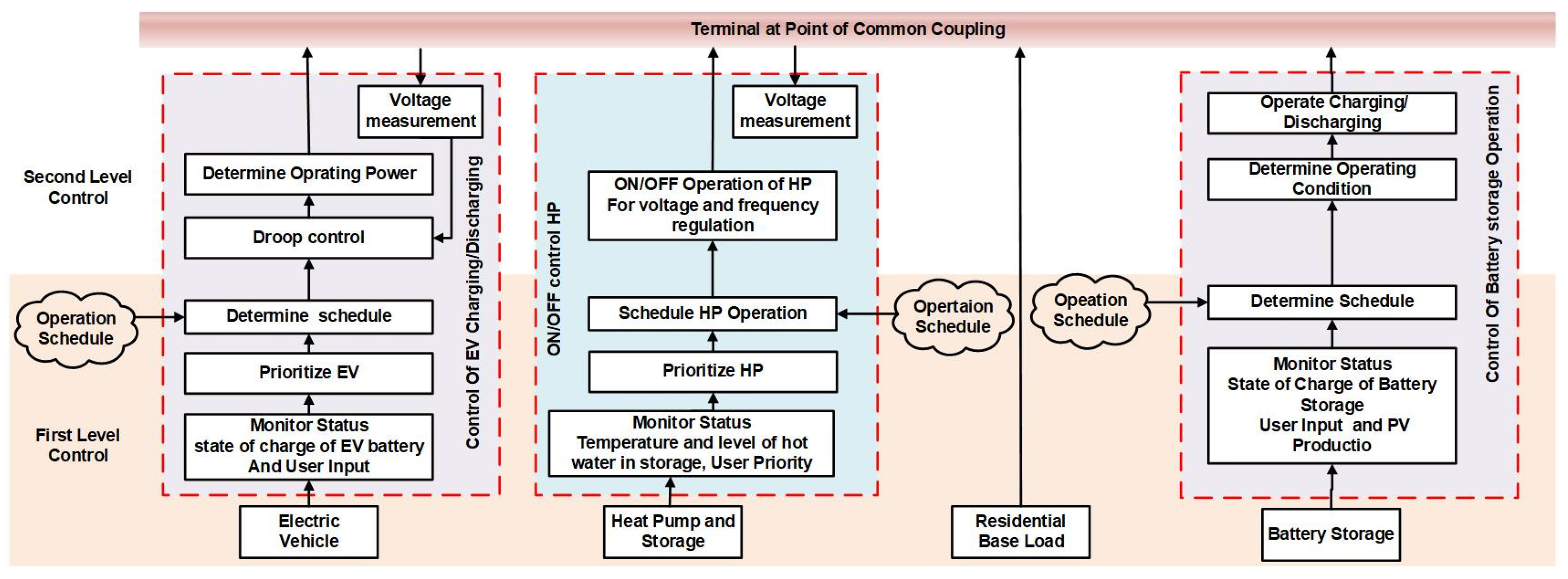
Figure 2.
Holistic CCMs of EV charging including droop control, scheduled charging, power regulation, and priority charging.
Figure 2.
Holistic CCMs of EV charging including droop control, scheduled charging, power regulation, and priority charging.
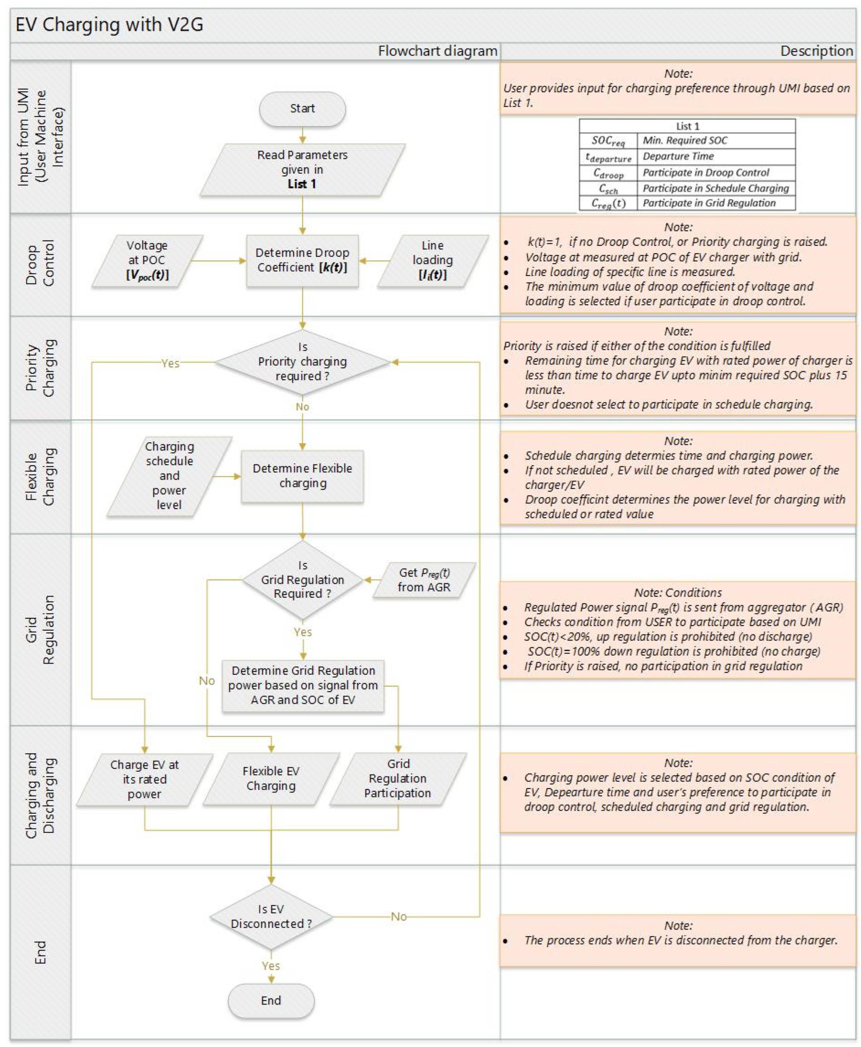
Figure 3.
Logic of EV charging to unlock flexibility through interaction with voltage at POC and transformer loading.
Figure 3.
Logic of EV charging to unlock flexibility through interaction with voltage at POC and transformer loading.
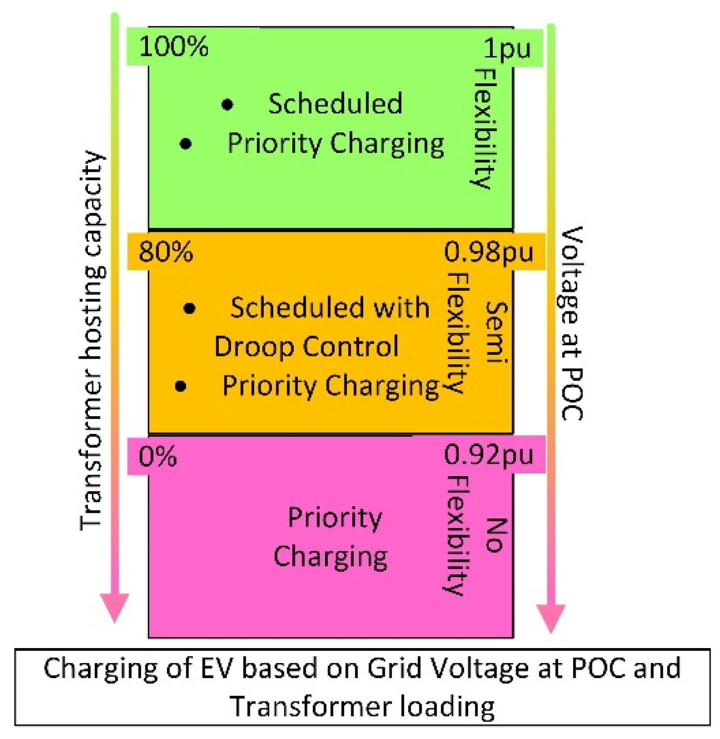
Figure 4.
Droop control coefficient for (a) bus voltage and (b) line loading.
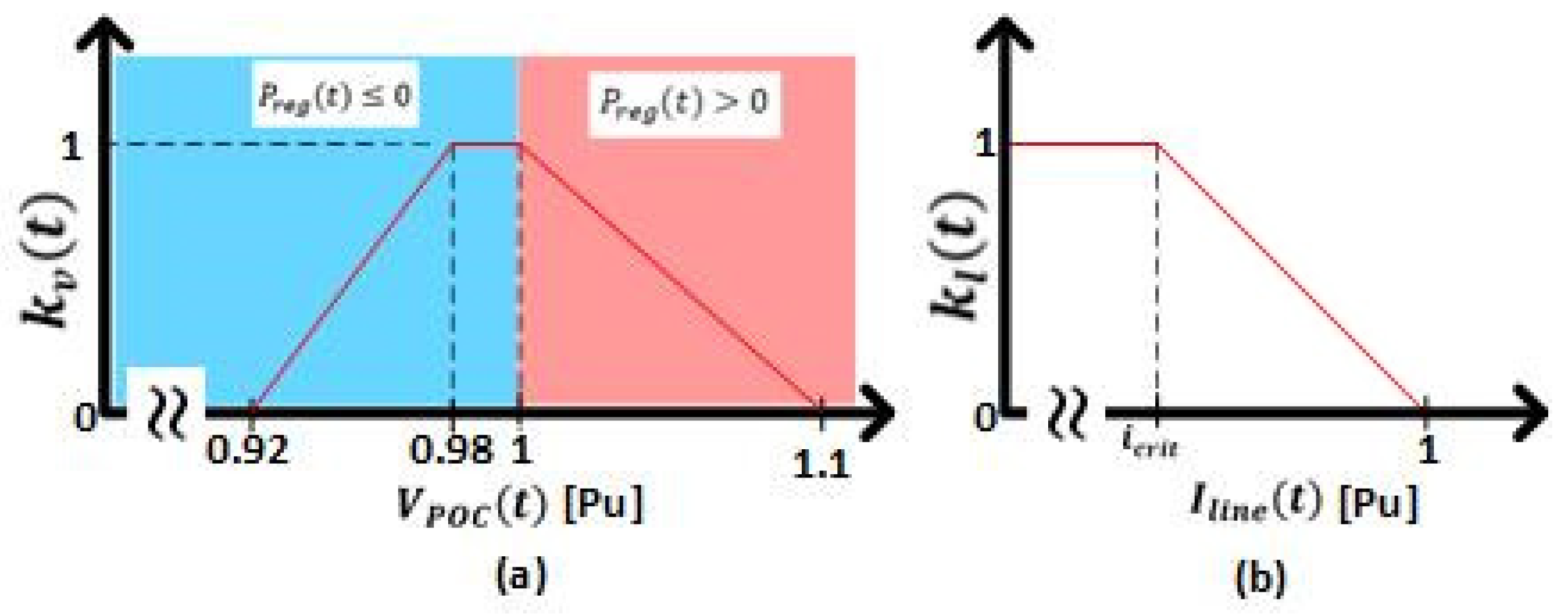
Figure 5.
Flowchart of CCMs for the PV-BESS.
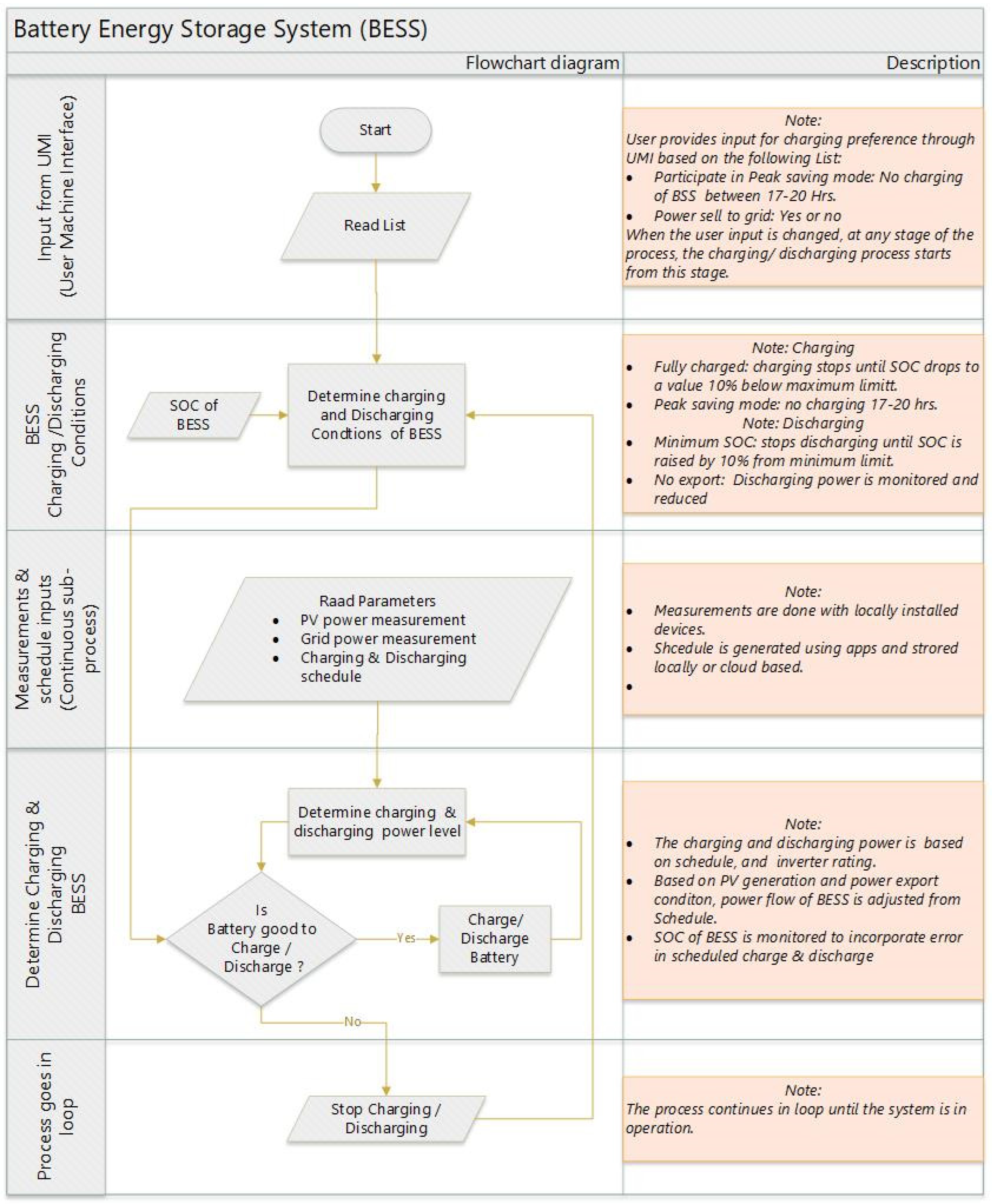
Figure 6.
Flexibility provision of the heating system in response to voltage magnitude.
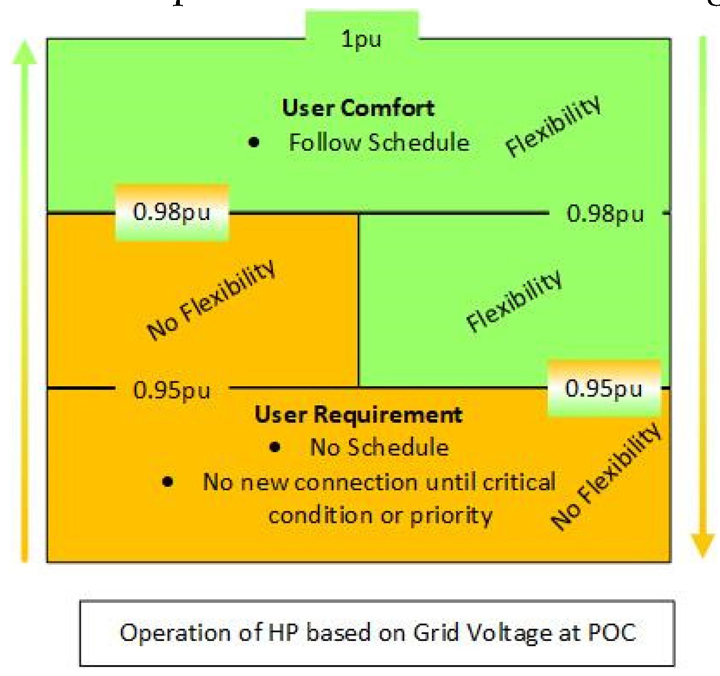
Figure 7.
Flowchart of the CCM for the heating system including HP and PCM.
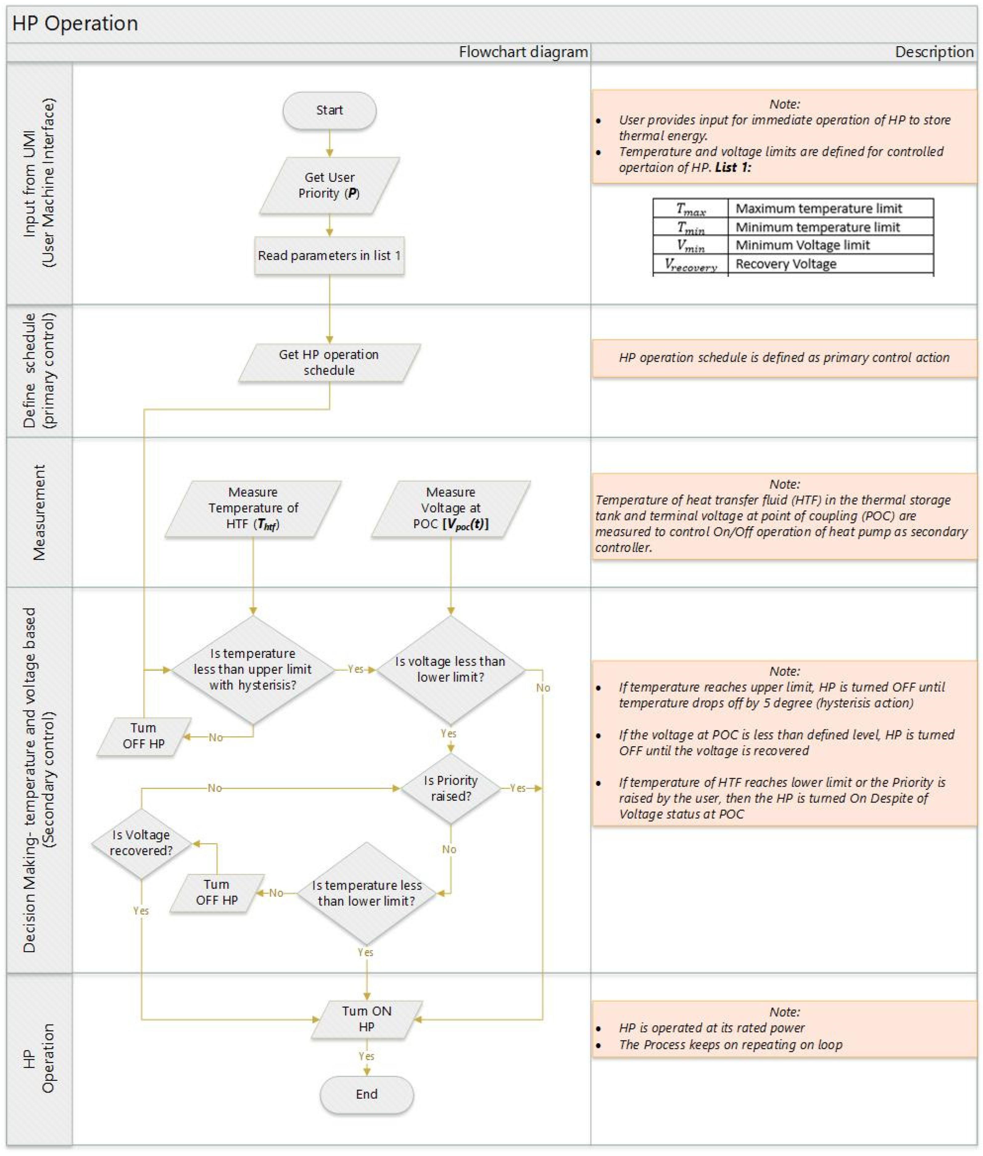
Figure 8.
Schematic diagram of a PCM storage with energy flows [36].
Figure 8.
Schematic diagram of a PCM storage with energy flows [36].
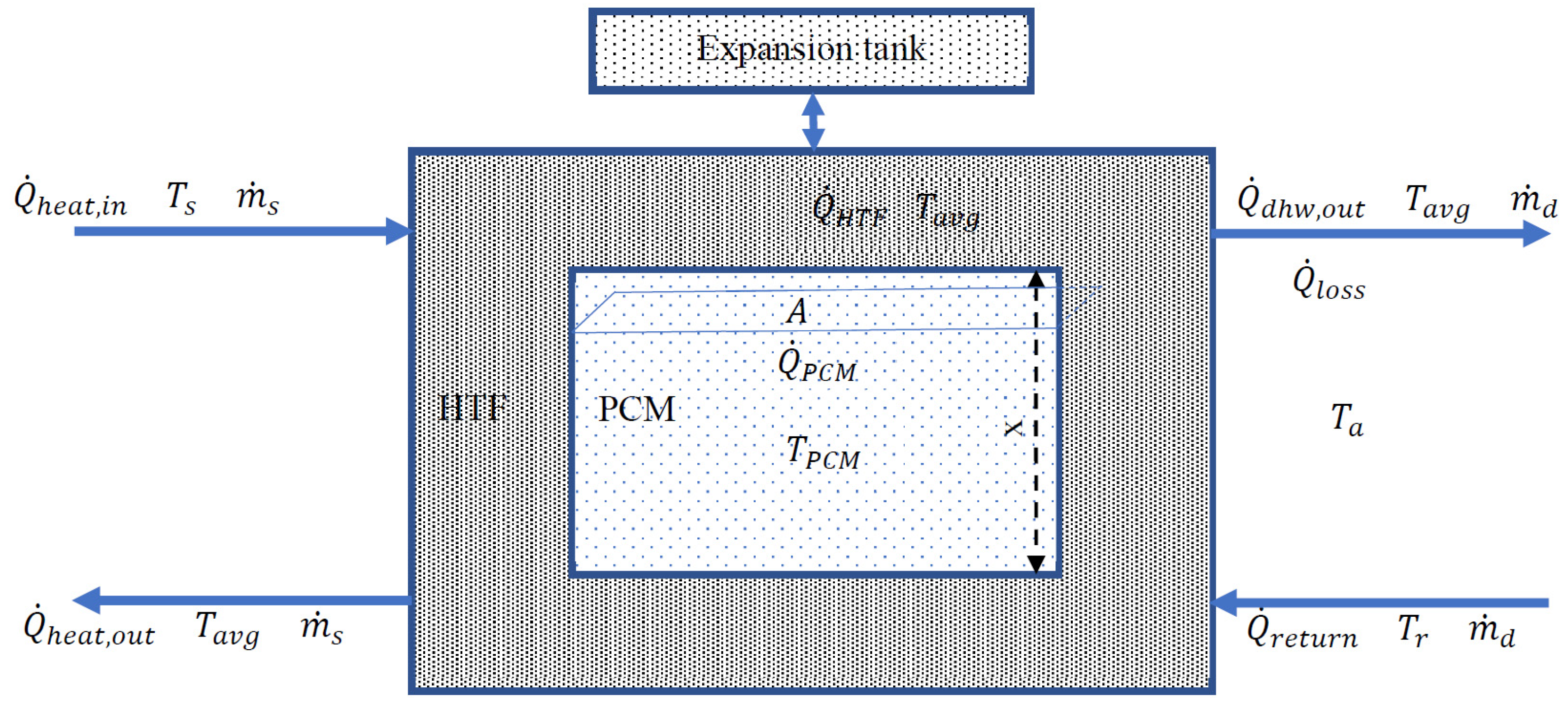
Figure 9.
The configuration of the 0.4 kV active distribution grid with flexible heat-power demands in DIgSILENT.
Figure 9.
The configuration of the 0.4 kV active distribution grid with flexible heat-power demands in DIgSILENT.
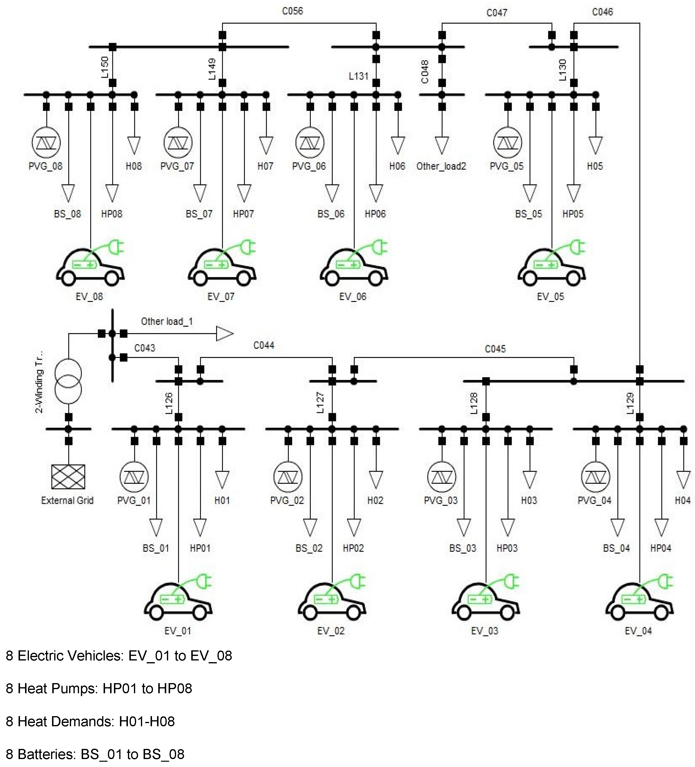
Figure 10.
Visualizing distribution grid’s dynamics in Case Study 1 (a) Active power of residential areas (b) Voltage magnitude at buses (c) Loading of the transformer (d) Line loading.
Figure 10.
Visualizing distribution grid’s dynamics in Case Study 1 (a) Active power of residential areas (b) Voltage magnitude at buses (c) Loading of the transformer (d) Line loading.
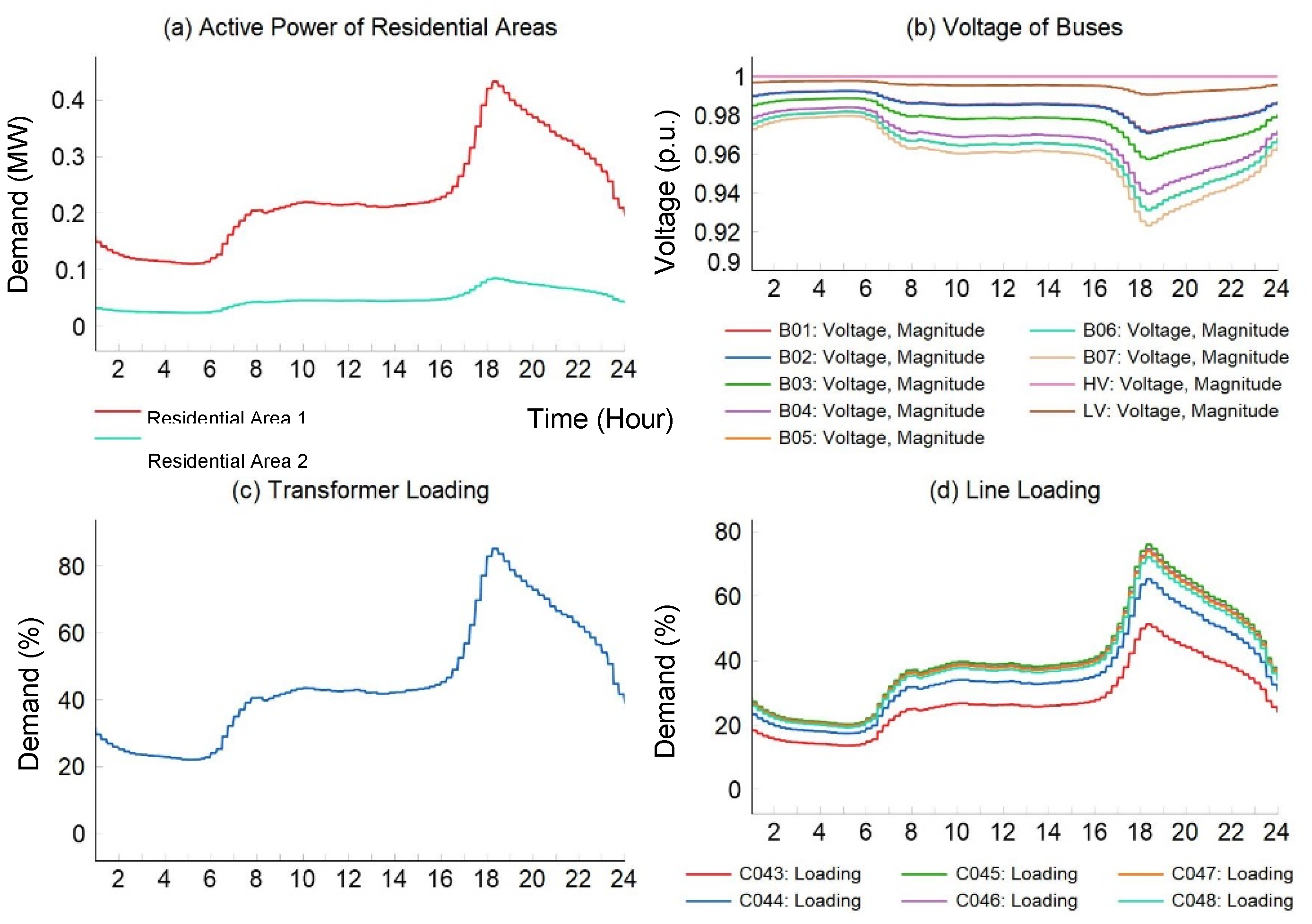
Figure 11.
Visualizing distribution grid’s dynamics in Case Study 2 (a) Temperature of PCM storage (b) Voltage magnitude at buses (c) Loading of the transformer (d) Line loading.
Figure 11.
Visualizing distribution grid’s dynamics in Case Study 2 (a) Temperature of PCM storage (b) Voltage magnitude at buses (c) Loading of the transformer (d) Line loading.
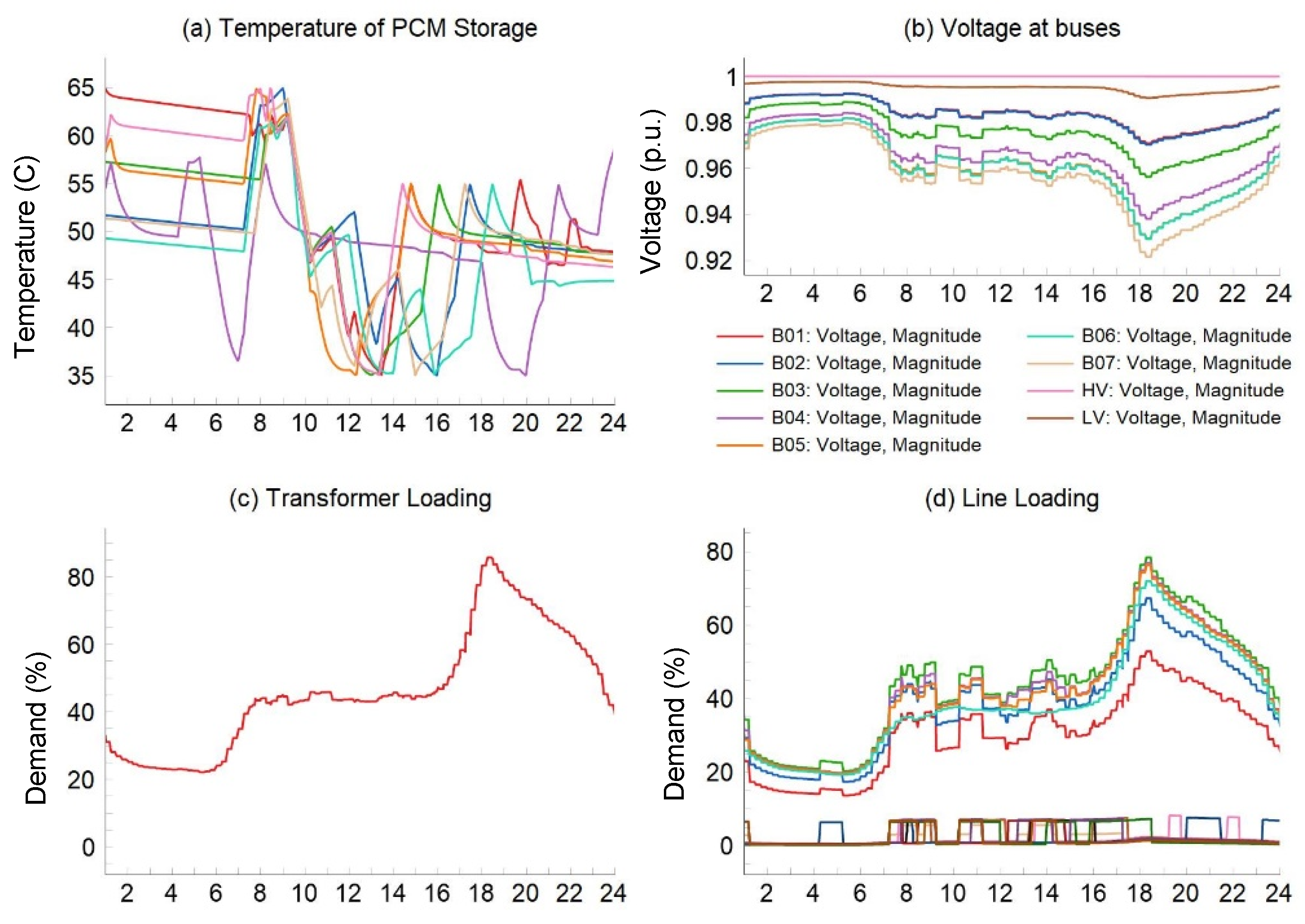
Figure 12.
Description of distribution grid’s dynamics in Case Study 3 (a) Temperature of PCM storage (b) Voltage magnitude at buses (c) Line loading (d) SOC of EV’s batteries.
Figure 12.
Description of distribution grid’s dynamics in Case Study 3 (a) Temperature of PCM storage (b) Voltage magnitude at buses (c) Line loading (d) SOC of EV’s batteries.
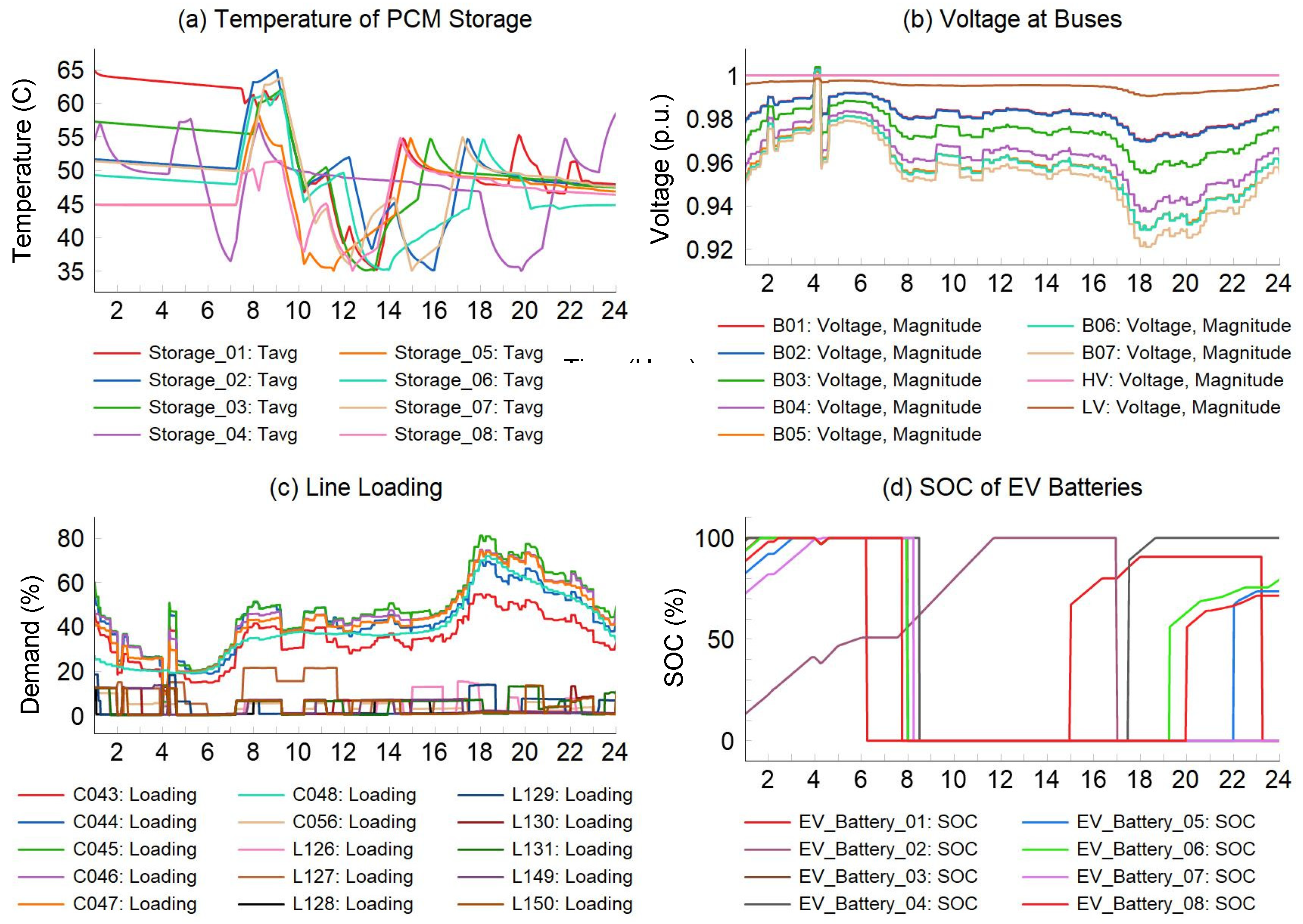
Figure 13.
Grid’s dynamics in Case Study 3-Scenario 1 (a) Loading of transformer (b) Voltage magnitude at buses (c) Line loading (d) SOC of EV’s batteries.
Figure 13.
Grid’s dynamics in Case Study 3-Scenario 1 (a) Loading of transformer (b) Voltage magnitude at buses (c) Line loading (d) SOC of EV’s batteries.
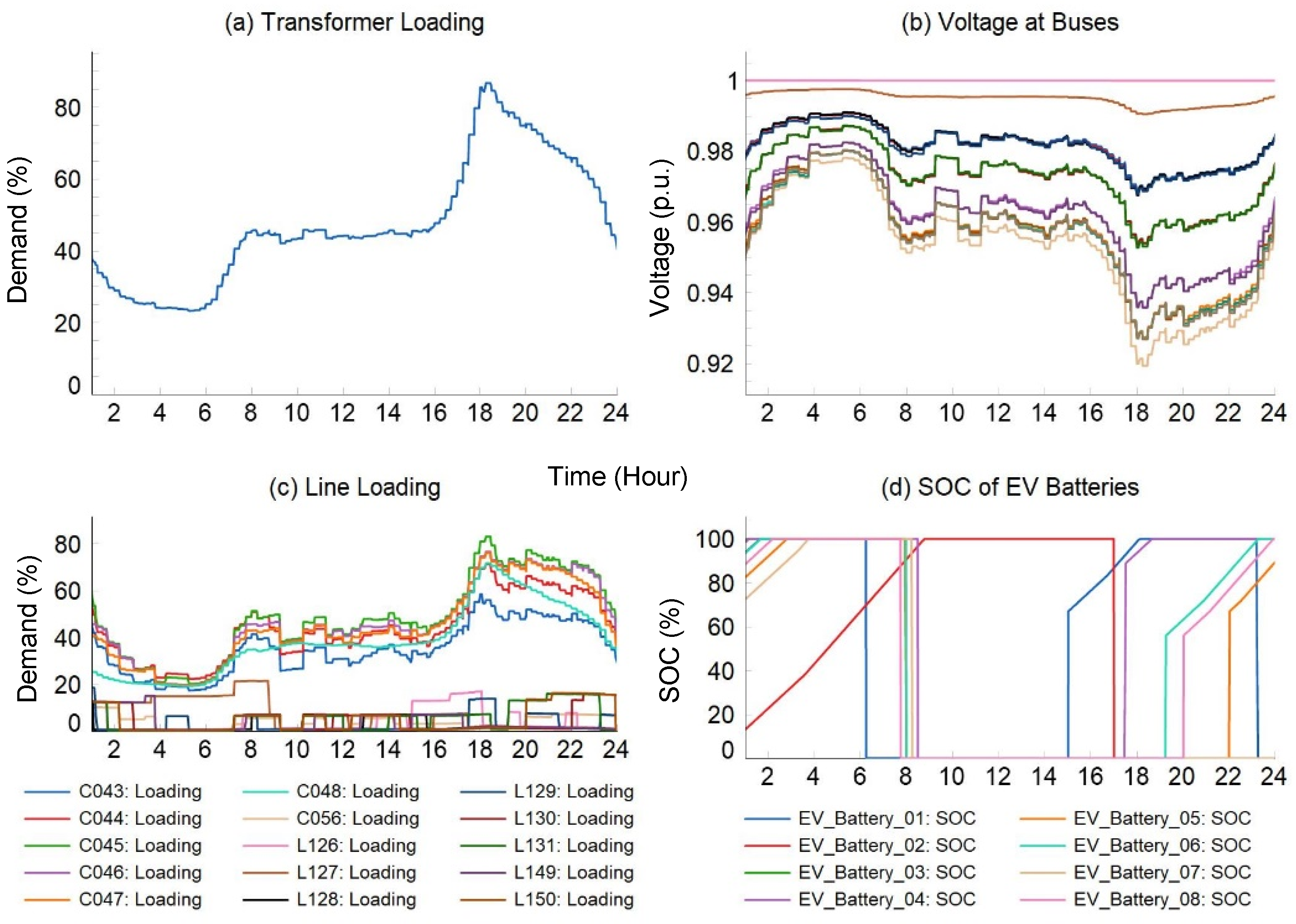
Figure 14.
Grid’s dynamics in Case Study 3-Scenario 2 (a) Loading of transformer (b) Voltage magnitude at buses (c) Line loading (d) SOC of EV’s batteries.
Figure 14.
Grid’s dynamics in Case Study 3-Scenario 2 (a) Loading of transformer (b) Voltage magnitude at buses (c) Line loading (d) SOC of EV’s batteries.
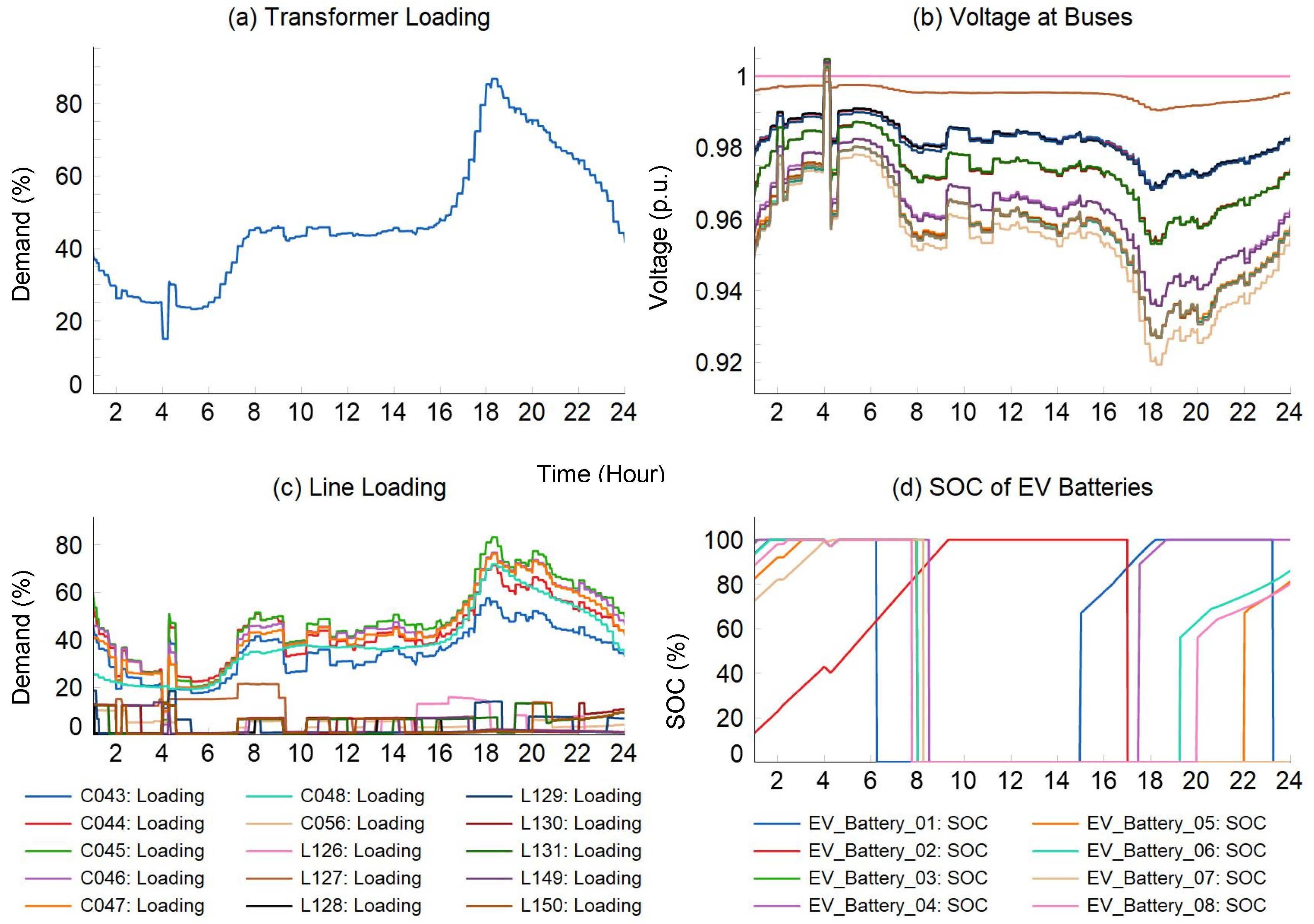
Figure 15.
Grid’s dynamics in Case Study 3-Scenario 3 (a) Loading of transformer (b) Voltage magnitude at buses (c) Line loading (d) SOC of EV’s batteries.
Figure 15.
Grid’s dynamics in Case Study 3-Scenario 3 (a) Loading of transformer (b) Voltage magnitude at buses (c) Line loading (d) SOC of EV’s batteries.
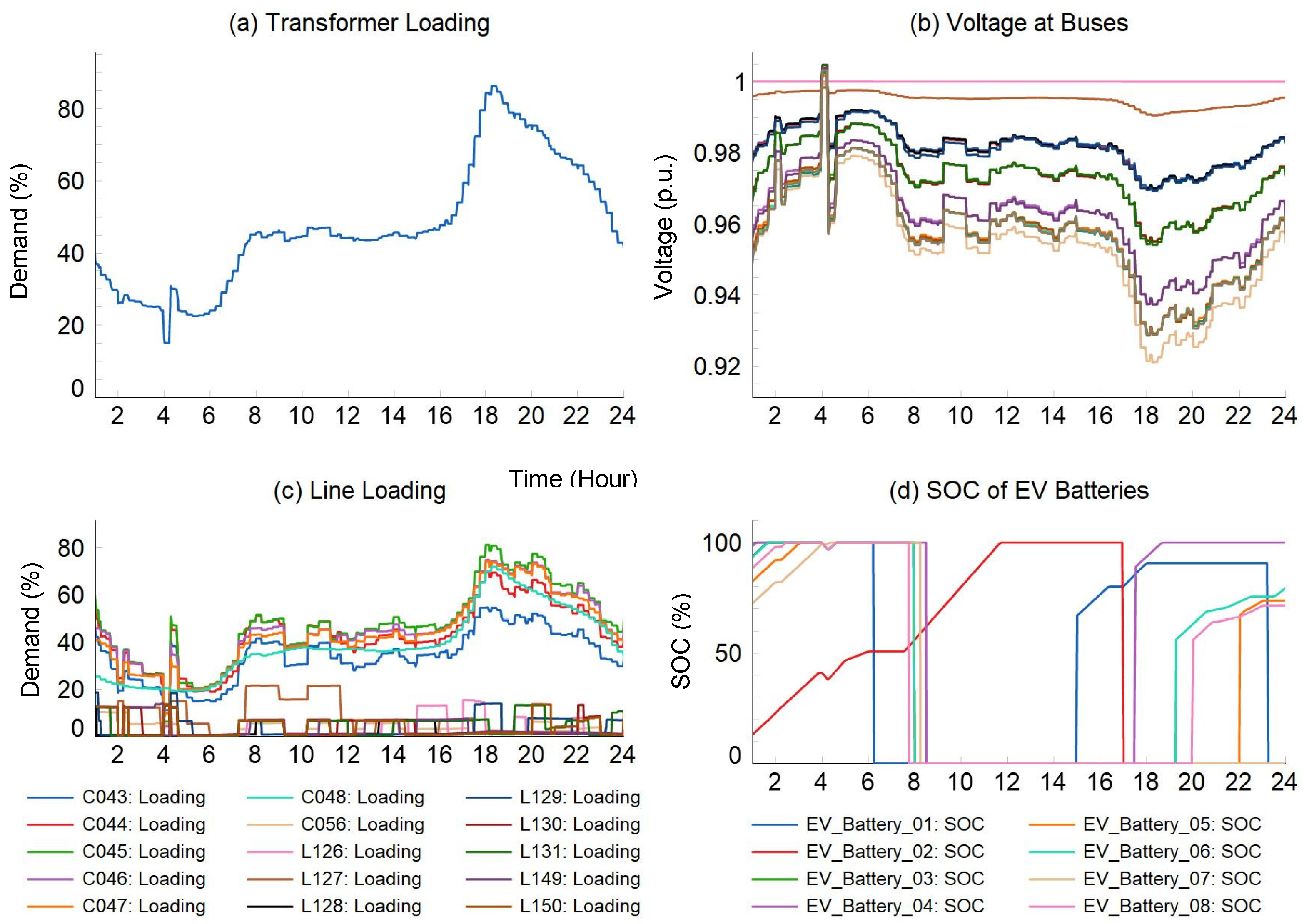
Figure 16.
Grid’s dynamics in Case Study 4 (a) Temperature of PCM storage (b) Voltage magnitude at buses (c) SOC of EV’s batteries (d) Active power generation of PV (e) Loading of the transformer (f) Line loading (g) SOC of batteries of BSS (h) Power transaction between households and grid.
Figure 16.
Grid’s dynamics in Case Study 4 (a) Temperature of PCM storage (b) Voltage magnitude at buses (c) SOC of EV’s batteries (d) Active power generation of PV (e) Loading of the transformer (f) Line loading (g) SOC of batteries of BSS (h) Power transaction between households and grid.
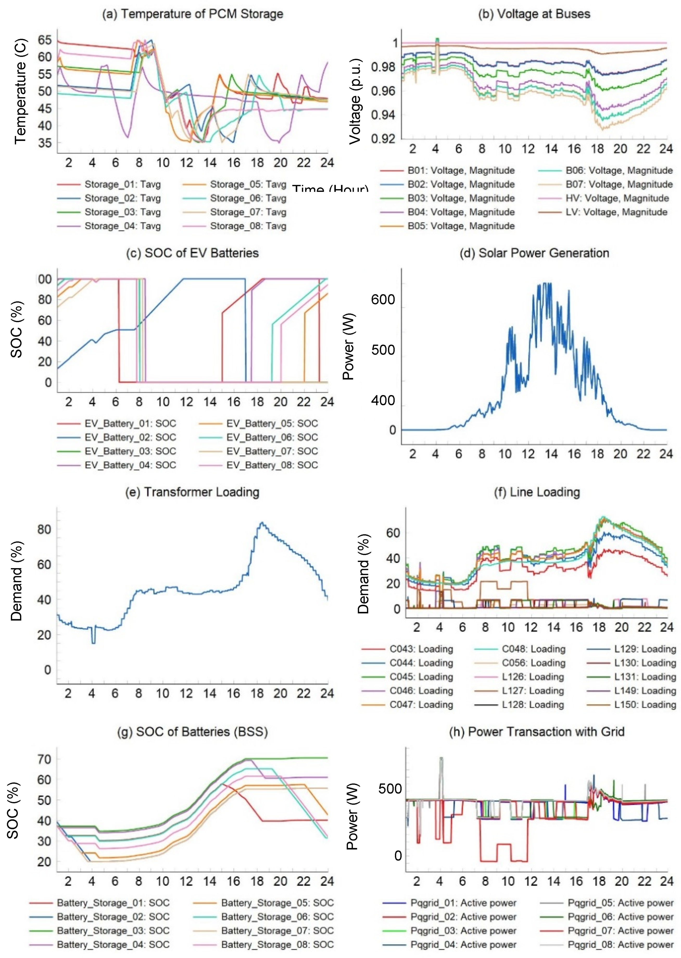
Figure 17.
Performance of secondary controller’s action in correcting errors of forecasted schedule for EV2 (a) SOC of EV2 (b) Control signal of priority charging (c) Regulation and scheduled charging power (d) Priority charging power.
Figure 17.
Performance of secondary controller’s action in correcting errors of forecasted schedule for EV2 (a) SOC of EV2 (b) Control signal of priority charging (c) Regulation and scheduled charging power (d) Priority charging power.
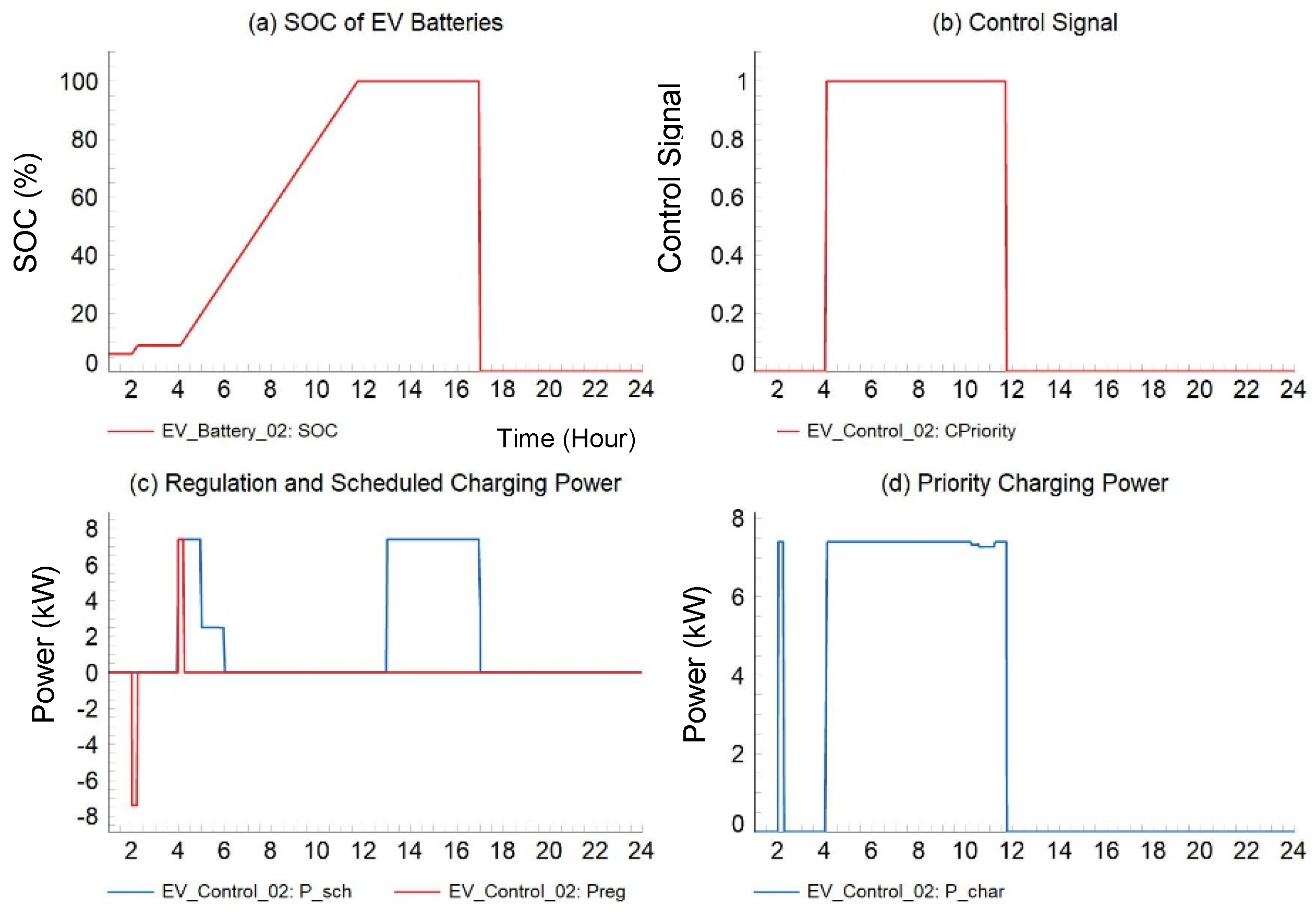

Table 1.
Technical parameters of the PCM thermal storage.
| Parameters | Unit | Value |
|---|---|---|
| Volume of storage tank | 0.5 | |
| Ratio of height to diameter | 3.25 | |
| Overall heat transfer coefficient of tank | 0.9 | |
| Ambient temperature in storage room | 10 | |
| Temperature of inflow cold water | 30 | |
| Total mass of hot water in the tank | 346.56 | |
| Thermal conductivity of PCM in solid state | 1 | |
| Thermal conductivity of PCM in liquid state | 0.6 | |
| Total mass of PCM in the storage | 170 | |
| Latent heat of fusion | 183000 | |
| Melting temperature | 49.5 | |
| Freezing temperature | 45 | |
| Specific heat capacity liquid | 3000 | |
| Specific heat capacity solid | 3000 | |
| Convective heat transfer coefficient | 60 | |
| Density of PCM | 1.3 | |
| Number of heat cells in the tank () | 548 |
Table 2.
Technical parameters of the HP.
| Parameters | Unit | Value |
|---|---|---|
| Thermal rating of Heat pump | 9 | |
| Flow rate from HP | (1.2-1.5) | |
| Flow rate from HP | 0.3-4.2 | |
| Flow in heating system (less than 10 ) | < 0.17 |
Table 3.
Technical parameters of the EV, PV, BESS.
| Parameters | Unit | Value |
|---|---|---|
| EV | ||
| EV Battery Size | 62 | |
| Rater Power of EV charger | 7.4 | |
| BESS | ||
| BESS Battery Size | 80 | |
| Rater Power of BESS inverter | 7.4 | |
| PV | ||
| Rated PV power | kW | 6 |
Table 4.
Voltage magnitude for all the case studies (NB: “×” included and “-” means excluded).
| Case Number | Included Flexible Demands | Ave. Voltage Magnitude (p.u.) | ||||
|---|---|---|---|---|---|---|
| HP | EV | PV-BSS | Peak Period | Whole Day | ||
| Case study 1 | - | - | - | 0.9641 | 0.9702 | |
| Case study 2 | × | - | - | 0.9635 | 0.9707 | |
| Case study 3 | Base Case | × | × | - | 0.9614 | 0.9719 |
| Scenario 1 | × | × | - | 0.9578 | 0.9755 | |
| Scenario 2 | × | × | - | 0.9593 | 0.9707 | |
| Scenario 3 | × | × | - | 0.9602 | 0.9710 | |
| Case study 4 | × | × | × | 0.9650 | 0.9742 | |
Disclaimer/Publisher’s Note: The statements, opinions and data contained in all publications are solely those of the individual author(s) and contributor(s) and not of MDPI and/or the editor(s). MDPI and/or the editor(s) disclaim responsibility for any injury to people or property resulting from any ideas, methods, instructions or products referred to in the content. |
© 2024 by the authors. Licensee MDPI, Basel, Switzerland. This article is an open access article distributed under the terms and conditions of the Creative Commons Attribution (CC BY) license (https://creativecommons.org/licenses/by/4.0/).
Copyright: This open access article is published under a Creative Commons CC BY 4.0 license, which permit the free download, distribution, and reuse, provided that the author and preprint are cited in any reuse.


