1. Introduction
The uplift of the Andes represents one of the most significant events in the biogeographic history of South America [
1], serving as a vicariant barrier, a biological corridor, and a source of new ecosystems and conditions in extra-Andean areas [
2,
3,
4,
5]. The influence of this mountain range on the climatic and biotic history is partly attributed to its impact on atmospheric circulation [
6], affecting the distribution of precipitation along the latitudinal gradient [
3].
Macroclimatic conditions, alongside diverse histories of colonization and in situ speciation, shape the zonal vegetation associated with the Andes, influencing its structure and composition [
2,
7]. In southern South America, a biogeographic break is observed near 27°S in the Andes, which divides the ecosystems of the Puna to the north and the Andean steppe to the south [
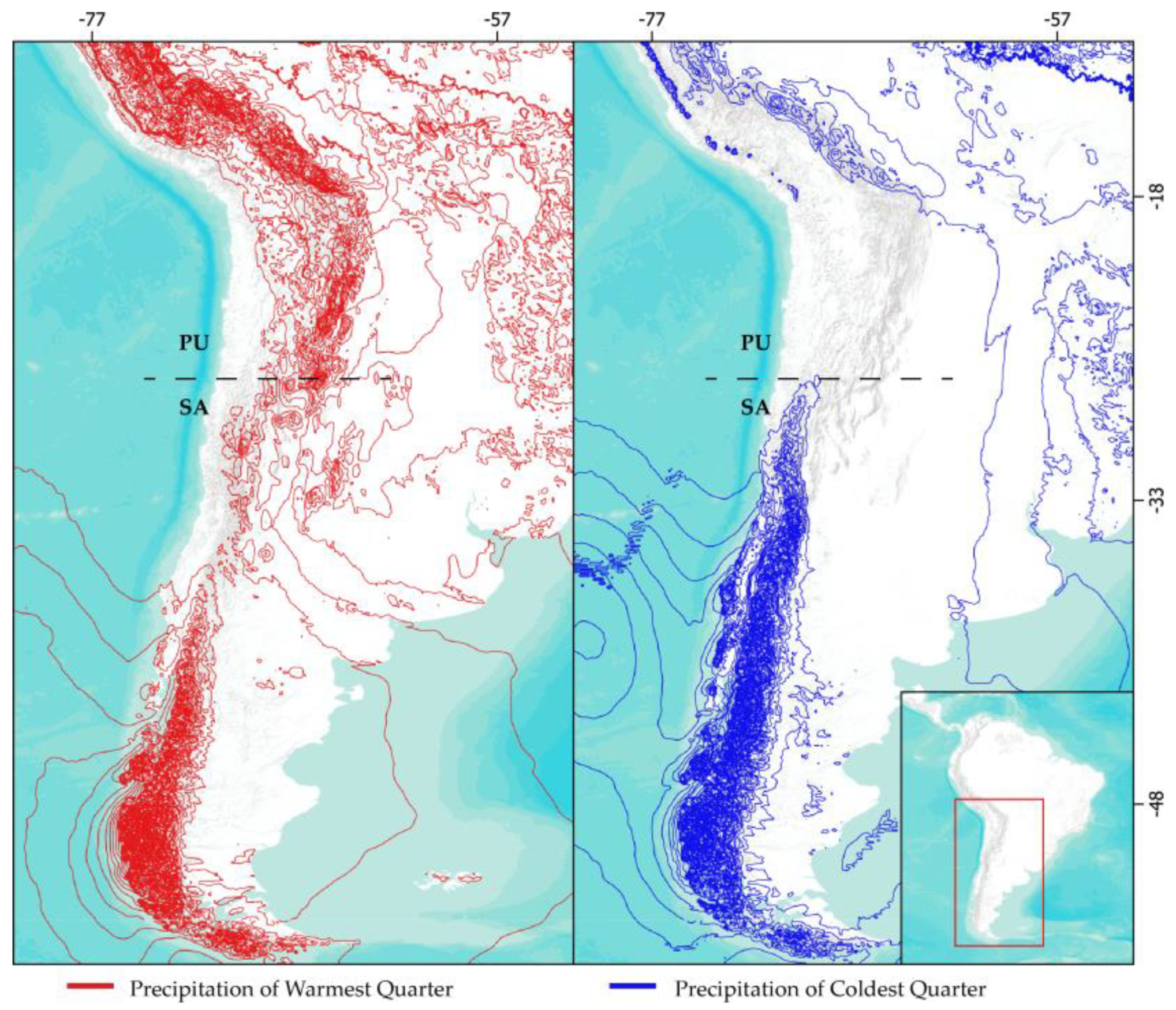
8]. Each is influenced by different precipitation regimes: summer rainfall from easterly winds and winter rainfall from westerly winds, respectively (
Figure 1) [
3,
8]. The aridity resulting from the shift between winter and summer precipitation regimes acts as an environmental filter that limits north-south dispersal, particularly around 29°S [
9]. This phenomenon correlates with a turnover of species, a decrease in richness, and changes in life forms [
9,
10,
11].
Additionally, microclimatic conditions emerge in the context of the interaction between Andean topography and the local environment [
12,
13], conducive to establishing azonal ecosystems such as Cushion Bogs [
8,
9]. These high Andean wetlands, also known as “Bofedales”, “Vegas”, or “Mallines” [
14,
15], develop near the hydrological and altitudinal limits for plant life in the Andes [
14] from Colombia/Venezuela to Patagonia [
15,
16,
17]. They are dominated by “bogs-forming” plants, which grow in compact cushions, capable of forming peat, retaining moisture, altering local hydrological conditions, and creating conditions for the colonization of other species [
15,
18,
19]. These plants, mainly Juncaceae like
Oxychloe,
Distichia, and
Patosia, along with Cyperaceae such as
Zameiocirpus [
15], show variations in their distribution. For instance,
Distichia dominates bogs with a tropical and subtropical distribution from Colombia to northern Chile and Argentina. At the same time,
Oxychloe is found in subtropical and extratropical distributions from southern Peru to central-southern Chile and Argentina [
20,
21].
Bogs represent a complex of different species interlocked with each other [
22,
23,
24]. Generally, the flora composing these ecosystems is characterized by rapid vegetative reproduction, high seed production, and both endozoochoric and epizoochoric dispersion [
15], as is the case with the dominant Juncaceae, which exhibit clear adaptations for dispersion by birds [
9]. Moreover, many of these species demonstrate an anemophilous pollination strategy, and a significant number are considered autogamous [
9]. It is proposed that these reproductive characteristics have played a crucial role in the homogeneity of bog flora compared to zonal flora along the latitudinal gradient, regardless of macroclimatic conditions [
9,
10]. However, bogs are affected by small-scale climatic conditions; for instance, the influence of elevation and temperature on the change in dominance of Juncaceae species has been documented [
15,
25,
26,
27,
28], as well as the effect of the physicochemical characteristics of associated waters [
9,
15,
16]. Moreover, significant impacts of human activity on floristic composition have been identified [
15,
22,
23], but above all, the aridity-humidity gradients have been proposed as the main factor shaping these communities’ composition [
9,
10,
15,
25,
26,
27,
29,
30].
The “Environmental Filters” hypothesis proposes that environmental factors restrict communities by selecting species through a hierarchical process from large-scale filters to microclimatic factors and biotic interactions [
31,
32], leaving a mark on the species composition of communities [
33,
34], that is, on beta diversity, a measure of the differences in species composition between communities [
35,
36]. Beta diversity can be broken down into two components: (1) turnover, which is the replacement of species between sites, and (2) nestedness, which refers to the loss of species from one site, transforming into a subset of another [
37,
38]. These components provide insights into the underlying processes driving differences in species composition. Turnover is generally associated with niche diversity along the study gradient, while nestedness is related to spatial variables and dispersal [
38,
39,
40].
Environmental filters also impact the phylogenetic structure of communities, manifesting in patterns of phylogenetic clustering, where community members are more closely related due, for instance, to shared traits for persistence in a particular environment [
41,
42]. In contrast, in the absence of environmental filters, a pattern of phylogenetic overdispersion emerges, where individuals are not closely related, and interactions predominate [
41,
43,
44,
45].
These backgrounds on the biogeographic patterns of zonal and azonal vegetation in the Andes, as well as the various environmental effects that influence the structure of communities, guide the research question in this work: What environmental filters explain the floristic composition of bogs on a large scale along the latitudinal gradient of southern South America? We hypothesize that the variation in precipitation patterns, particularly between the northern macroclimatic areas, dominated by summer rains, southern areas, dominated by winter rains, and the transition between both precipitation regimes, differentiates the bog communities along the latitudinal gradient of their distribution.
Accordingly, it is predicted: (1) An increase in beta diversity towards the extremes of the latitudinal gradient, primarily due to species turnover or rotation; (2) Clustering of communities, based on beta diversity, that differentiates the macroclimatic regions north, transition, and south of the precipitation regimes; (3) Greater overlap of climatic niches among species within regions than between macroclimatic regions; and (4) Phylogenetic clustering in communities within each macroclimatic region. This study aims to determine the influence of environmental filters on the differentiation on a large scale of bog communities along the latitudinal gradient of the Andes.
5. Conclusions
This study provided a comprehensive assessment of how macro-environmental variables function as filters in the differentiation of communities in bogs along the Andes (15°S - 41°S). The findings indicate a low total beta diversity across this gradient, primarily influenced by dispersal limitations and macro-environmental conditions. Three distinct bioregions were identified based on taxonomic diversity, corresponding to the macroclimates of Chile and the phytogeographic districts of the high Andean province of southern South America.
Notably, species at the extremes of the north-south gradient exhibited significant differences in their climatic niches, with a broader niche width in the transition zone. Phylogenetic metric analyses indicate clustering between rainfall regimes in the arid transition zone, reflecting phylogenetic conservatism in niche preference.
In conclusion, this study validates the proposed hypothesis by identifying a clear separation of communities in the transition of rainfall regimes. However, it adds temperature variation as an influential factor in community formation. Significantly, macro-environmental conditions exert a considerable effect on the biodiversity of azonal flora in the Southern Andes of South America, playing a critical role in shaping these unique communities.
Figure 1.
Map of the precipitation regimes in southern South America represented by Precipitation of Warmer Quarter (red lines) and Precipitation of Coldest Quarter (blue lines). Dotted lines divide the Puna (PU) and southern Andean steppe (SA) ecosystems.
Figure 1.
Map of the precipitation regimes in southern South America represented by Precipitation of Warmer Quarter (red lines) and Precipitation of Coldest Quarter (blue lines). Dotted lines divide the Puna (PU) and southern Andean steppe (SA) ecosystems.
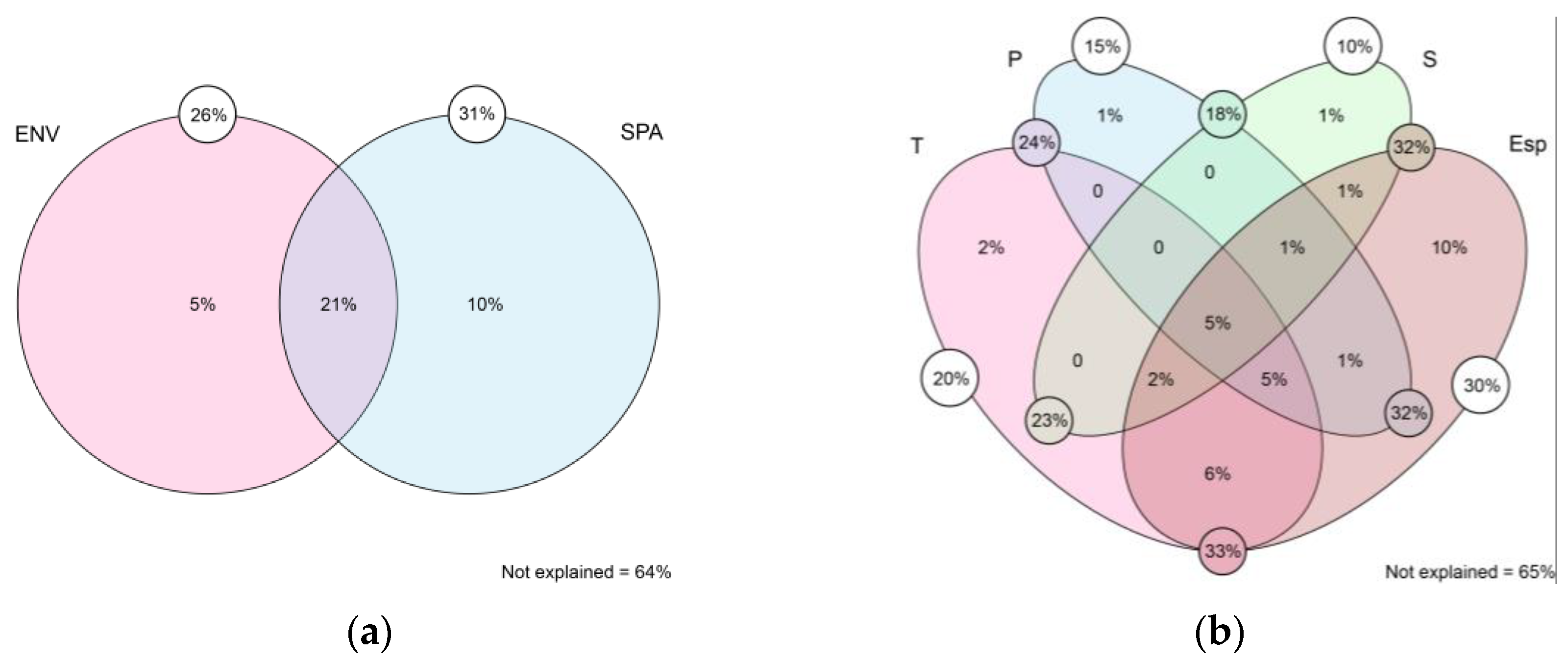
Figure 2.
Venn diagram of the variance partitioning analysis between environmental and spatial factors (a) and between each environmental component with spatial factors (b). The values inside each circle/oval indicate the individual contribution of that variable. The values in the small white circles indicate the contribution of the variable considering a synergistic effect with the others. The values in the small circles colored according to the intersection correspond to the contribution of the interaction of those two variables, considering the synergistic effect with the others. ENV = environment; SPA = spatial; T = temperature; P = precipitation; S = soil.
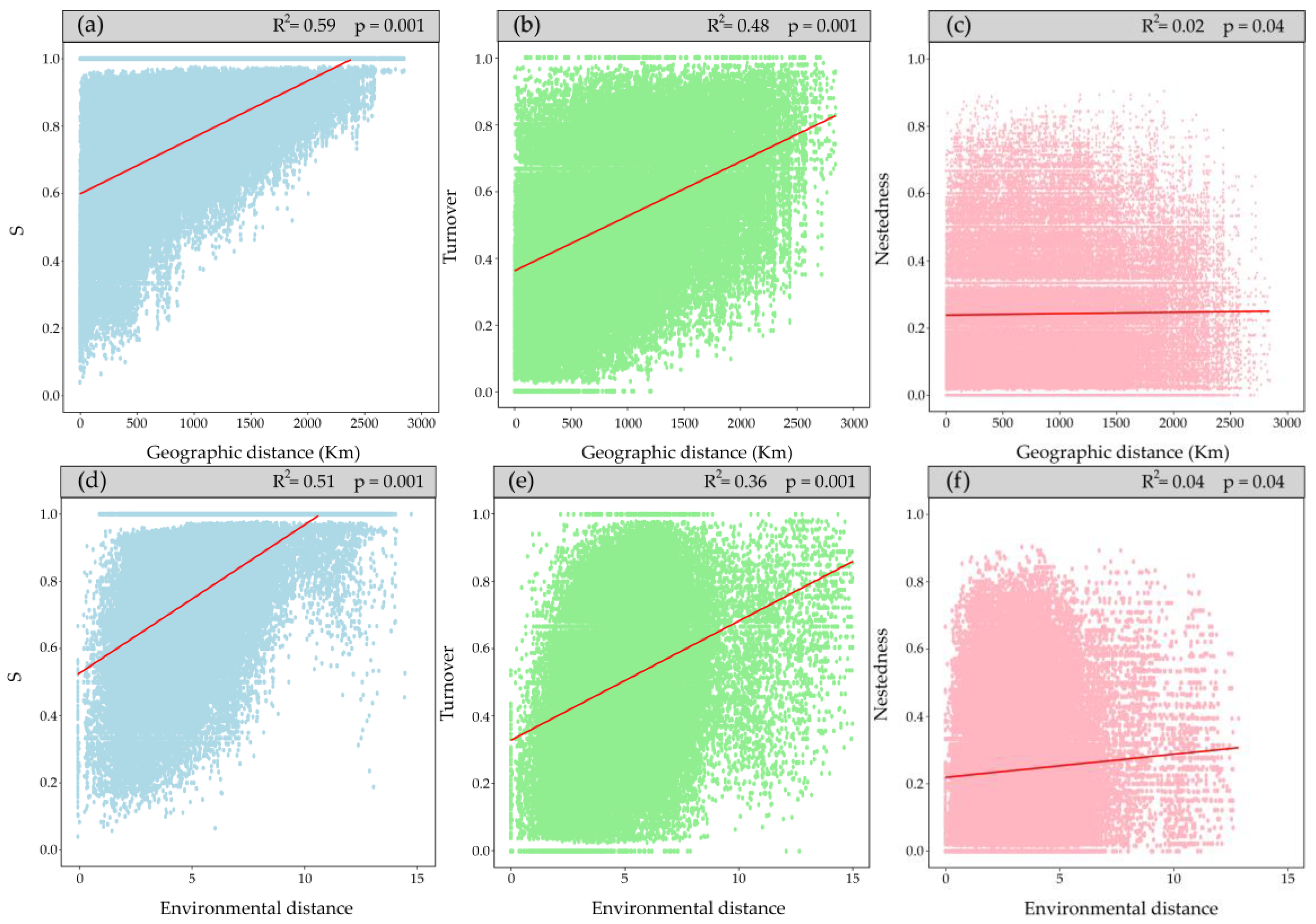
Figure 3.
The first row (a, b, c) shows the relationships between beta diversity and its components with geographic distance. The second row (d, e, f) shows the relationships between beta diversity and its components with environmental distance.
Figure 3.
The first row (a, b, c) shows the relationships between beta diversity and its components with geographic distance. The second row (d, e, f) shows the relationships between beta diversity and its components with environmental distance.
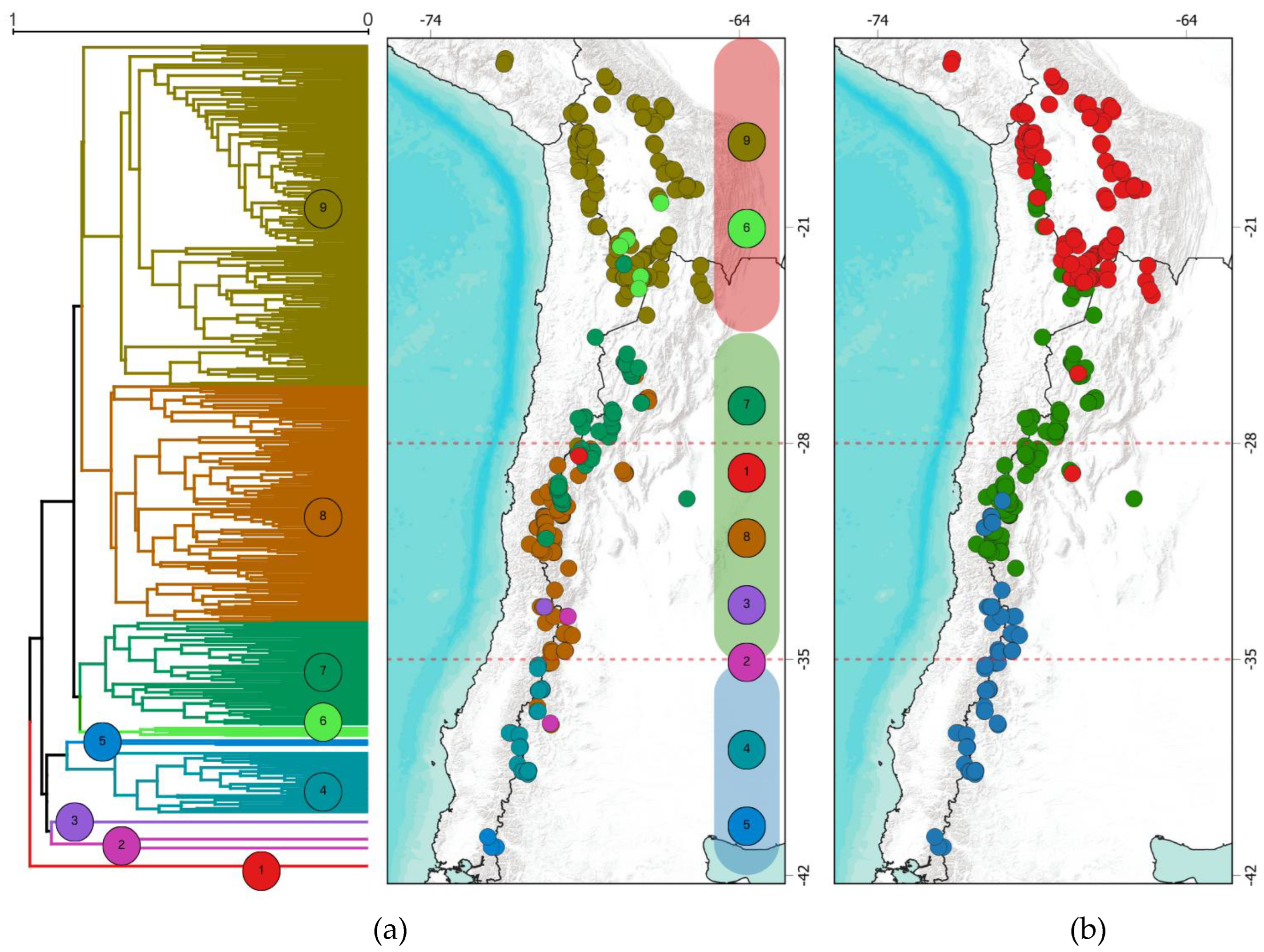
Figure 4.
Dendrogram of floristic affinities based on the Sorensen dissimilarity index with its projection onto geographic space in (a). Regionalization by membership grade model in (b). The dotted red lines correspond to the operational macrozones defined in this study.
Figure 4.
Dendrogram of floristic affinities based on the Sorensen dissimilarity index with its projection onto geographic space in (a). Regionalization by membership grade model in (b). The dotted red lines correspond to the operational macrozones defined in this study.
Figure 5.
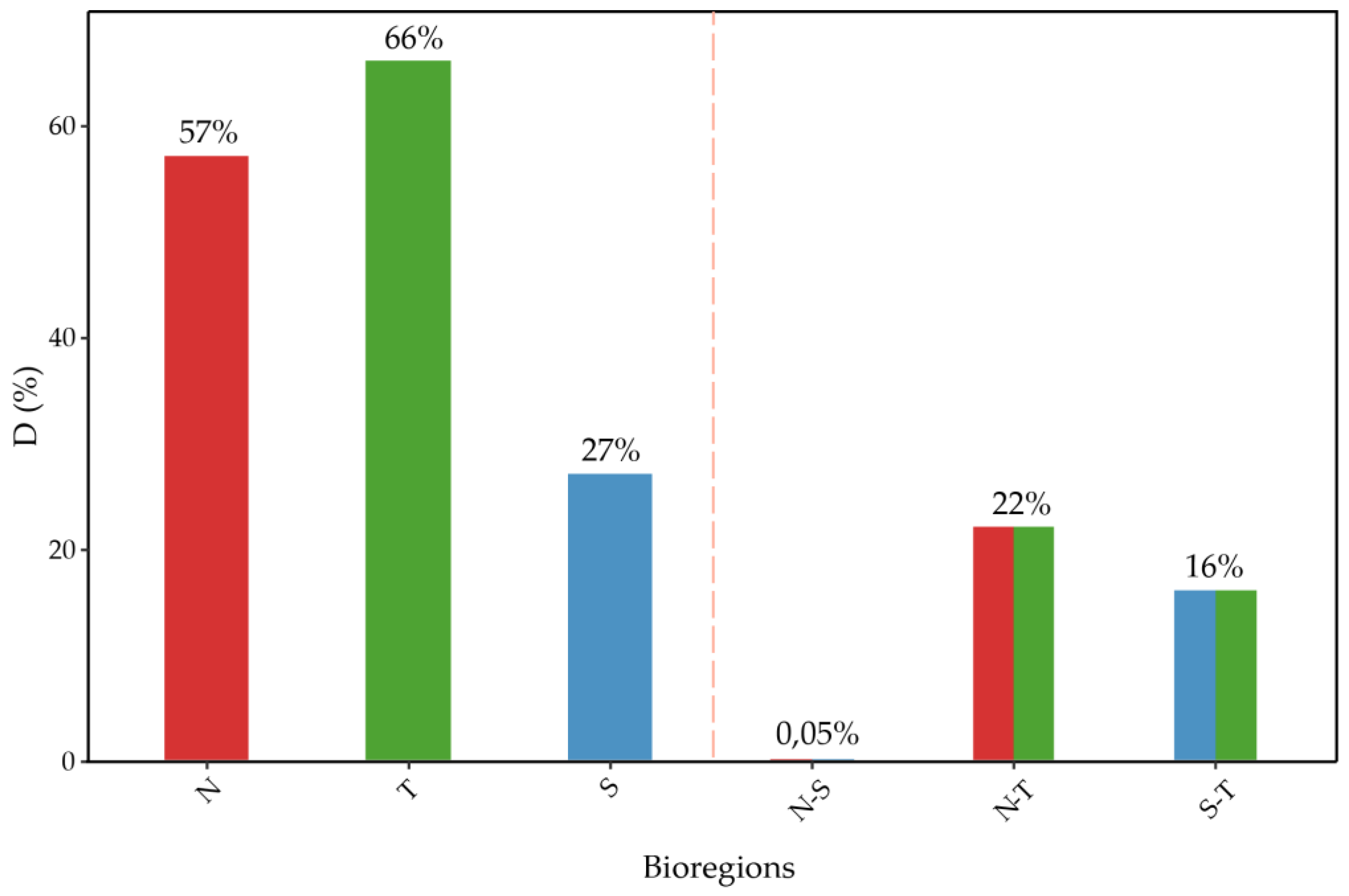
Average “D” Overlap Index as a percentage for species from each bioregion. “N” represents the average overlap among species within the northern bioregion; “T” indicates the average overlap among species within the transition bioregion; “S” refers to the average overlap among species within the southern bioregion. “N-S” denotes the average overlap between species from the north and south bioregions; “N-T” refers to the average between species from the northern and transition bioregions; “S-T” shows the average between species from the southern and transition bioregions.
Figure 6.
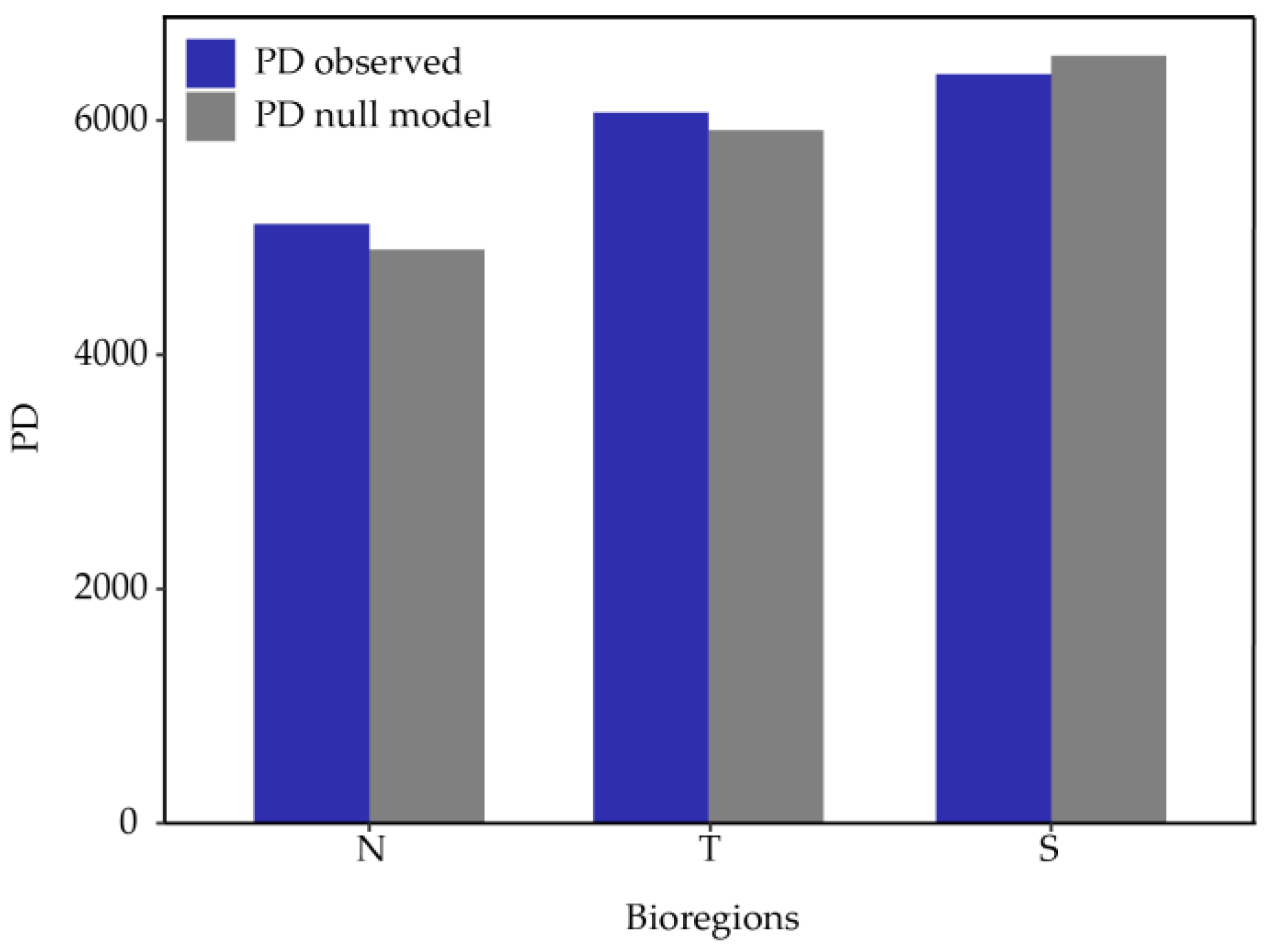
Observed Phylogenetic Diversity (PD) for each bioregion (blue) and expected PD according to the null model (gray).
Figure 6.
Observed Phylogenetic Diversity (PD) for each bioregion (blue) and expected PD according to the null model (gray).
Figure 7.
Observed Phylogenetic Diversity (PD) for each 2° latitudinal band (blue) and the expected PD according to the null model (gray).
Figure 7.
Observed Phylogenetic Diversity (PD) for each 2° latitudinal band (blue) and the expected PD according to the null model (gray).
Figure 8.
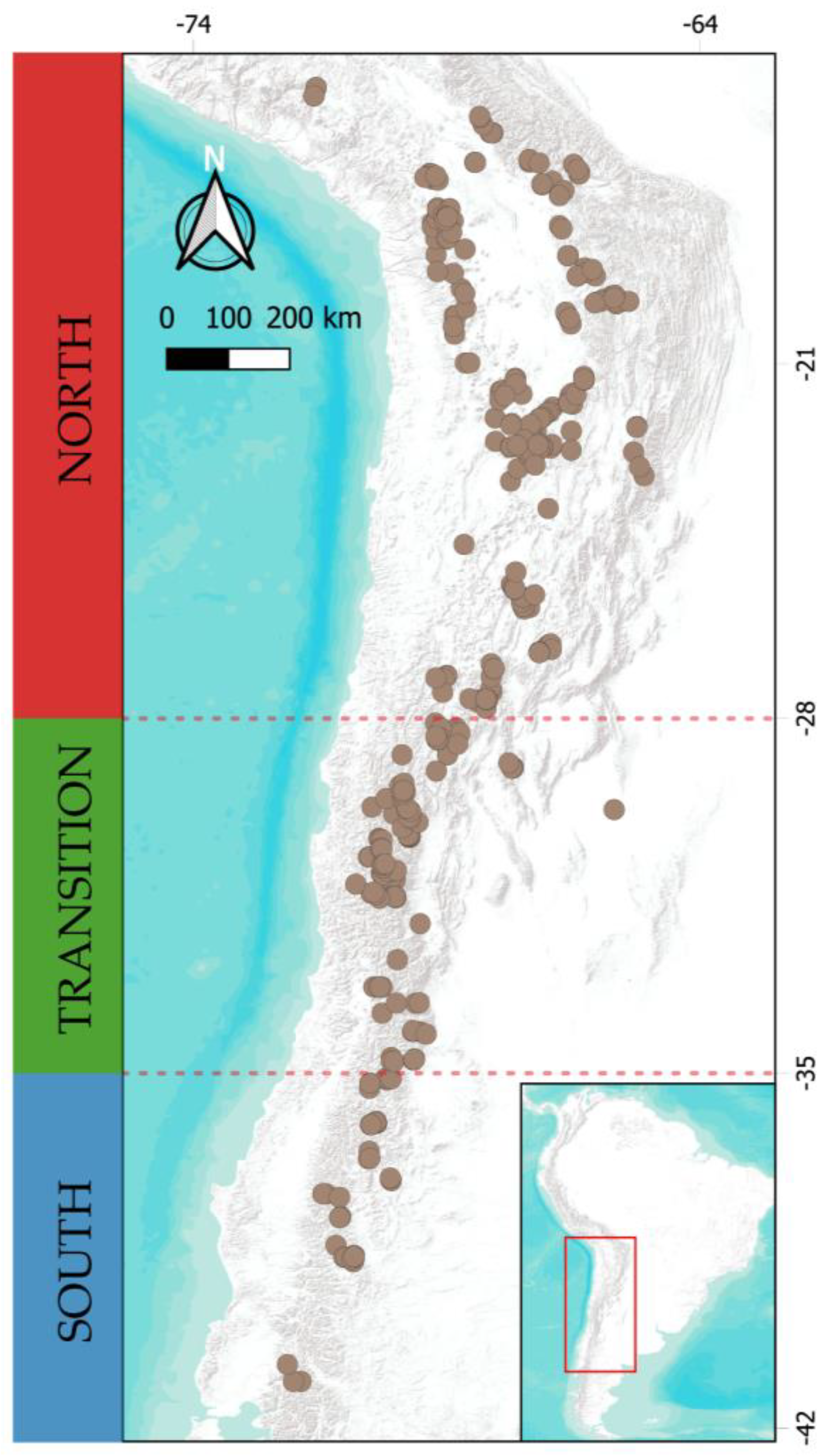
Distribution map of the 420 bogs in southern South America with the macroclimatic regions defined for this study: North (N), Transition (T), and South (S).
Figure 8.
Distribution map of the 420 bogs in southern South America with the macroclimatic regions defined for this study: North (N), Transition (T), and South (S).
Table 1.
Standardized effects of PD, MPD, and MNTD compared to the null model (z-score) for each bioregion with statistical significance (α).
Table 1.
Standardized effects of PD, MPD, and MNTD compared to the null model (z-score) for each bioregion with statistical significance (α).
| Bioregion |
PD z-score |
αPD |
MPD z-score |
αMPD |
MNTD z-score |
αMNTD |
| N |
0.771 |
0.773 |
1.899 |
0.979 |
0.462 |
0.678 |
| T |
0.523 |
0.683 |
1.430 |
0.949 |
0.275 |
0.591 |
| S |
-0.596 |
0.277 |
-1.310 |
0.142 |
-0.503 |
0.305 |
Table 2.
Standardized PD, MPD, and MNTD effects relative to the null model (z-score) for each 2° latitudinal band with statistical significance (α).
Table 2.
Standardized PD, MPD, and MNTD effects relative to the null model (z-score) for each 2° latitudinal band with statistical significance (α).
| Band |
PD z-score |
αPD |
MPD z-score |
αMPD |
MNTD z-score |
αMNTD |
| 15-16 |
0.386 |
0.658 |
1.507 |
0.859 |
0.343 |
0.659 |
| 17-18 |
1.041 |
0.836 |
1.740 |
0.931 |
1.291 |
0.879 |
| 18-19 |
1.738 |
0.953 |
2.141 |
0.982 |
1.681 |
0.943 |
| 21-22 |
0.189 |
0.608 |
1.866 |
0.932 |
0.243 |
0.598 |
| 23-24 |
-1.786 |
0.022 |
-0.912 |
0.126 |
-1.408 |
0.078 |
| 25-26 |
-0.783 |
0.231 |
-0.452 |
0.371 |
-0.546 |
0.304 |
| 27-28 |
-0.570 |
0.309 |
-0.558 |
0.305 |
-0.721 |
0.249 |
| 29-30 |
-1.452 |
0.064 |
-0.266 |
0.515 |
-1.517 |
0.059 |
| 31-32 |
-0.904 |
0.186 |
-0.805 |
0.179 |
-0.292 |
0.408 |
| 33-34 |
-0.562 |
0.295 |
-0.090 |
0.609 |
-0.809 |
0.215 |
| 35-36 |
-0.887 |
0.189 |
-0.587 |
0.322 |
-1.319 |
0.089 |
| 37-38 |
-0.344 |
0.376 |
-0.736 |
0.265 |
0.232 |
0.594 |
| 40-41 |
0.504 |
0.713 |
-0.435 |
0.388 |
0.637 |
0.747 |
Table 3.
Environmental Variables and Their Abbreviations Used in This Study.
Table 3.
Environmental Variables and Their Abbreviations Used in This Study.
| Type |
Variable (abbreviation) |
| Climate |
Annual Mean Temperature (Bio1) |
Mean Temperature of Coldest Quarter (Bio11) |
| Mean Diurnal Range (Bio2) |
Annual Precipitation (Bio12) |
| Isothermality (Bio3) |
Precipitation of Wettest Month (Bio13) |
| Temperature Seasonality (Bio4) |
Precipitation of Driest Month (Bio14) |
| Max Temperature of Warmest Month (Bio5) |
Precipitation Seasonality (Bio15) |
| Min Temperature of Coldest Month (Bio6) |
Precipitation of Wettest Quarter (Bio16) |
| Temperature Annual Range (Bio7) |
Precipitation of Driest Quarter (Bio17) |
| Mean Temperature of Wettest Quarter (Bio8) |
Precipitation of Warmest Quarter (Bio18) |
| Mean Temperature of Driest Quarter (Bio9) |
Precipitation of Coldest Quarter (Bio19) |
| Mean Temperature of Warmest Quarter (Bio10) |
|
| Edaphic |
Soil organic carbon in fine earth (Soc) |
Total nitrogen (Nitrogen) |
| Bulk density of the fine earth fraction (Bdod) |
Vol. fraction of coarse fragments (> 2 mm) (Cfvo) |
| pH H2O (Phh2o) |
Densidad de carbono orgánico (Ocd) |
| Silt (Silt) |
Sand (Sand) |
| Clay (Clay) |
|
| Elevación |
Digital elevation model (Elev) |
|
Table 4.
Environmental variables after correlation analysis and Forward Selection used for Variation Partitioning.
Table 4.
Environmental variables after correlation analysis and Forward Selection used for Variation Partitioning.
| |
Type |
Variables |
| Environment |
Temperature |
Bio2$$Bio7$$Bio9$$Bio10$$Bio11 |
| |
| |
| |
| |
| Precipitation |
Bio15$$Bio18 |
| |
| Edaphic |
Bdod$$Phh2o$$Cfvo |
| |
| |
| Spatial |
Elevation |
Elev |
| MEM |
4 |
1 |
3 |
| 5 |
9 |
8 |
| 2 |
12 |
51 |
| 19 |
17 |
10 |
| 32 |
59 |
28 |
| 11 |
37 |
6 |
| 16 |
40 |
24 |
| 23 |
20 |
33 |
| 22 |
52 |
42 |
| |
31 |
36 |
|
Table 5.
Equations Used for Calculating Beta Diversity. In (1), (3), and (4), a = species shared by the compared sites; b = species present exclusively in one site; and c = species present exclusively in the other site. In (2), n = sites in the dissimilarity matrix, created from equation (1); D2hi = √S between each site.
| Index |
Equation |
Source |
|
| S (Sorensen) |
|
(Chao et al., 2006) |
(1) |
| BDtotal |
|
(Legendre, 2013) |
(2) |
| Turnover(ReplS) |
|
(Legendre, 2014) |
(3) |
| Nestedness(RichDiffS) |
|
(Legendre, 2014) |
(4) |
Table 6.
Environmental Variables After Correlation Analysis and Forward Selection Used for Mantel Tests.
Table 6.
Environmental Variables After Correlation Analysis and Forward Selection Used for Mantel Tests.
| Type |
S |
Turnover |
Nestedness |
| Temperature |
Bio2 |
Bio2 |
Bio11 |
| |
Bio7 |
Bio7 |
|
| |
Bio9 |
Bio9 |
|
| |
Bio10 |
Bio10 |
|
| |
Bio11 |
Bio11 |
|
| Precipitation |
Bio15 |
Bio14 |
Bio16 |
| |
Bio16 |
Bio15 |
|
| |
Bio18 |
Bio16 |
|
| Edaphic |
Bdod |
Bio18 |
Silt |
| |
Phh2o |
Bdod |
Bdod |
| |
Silt |
Phh2o |
Soc |
| |
Sand |
Silt |
|
| |
Cfvo |
Cfvo |
|
| Elevation |
Elev |
Elev |
|
Table 7.
Selected Species for Niche Overlap Analysis.
Table 7.
Selected Species for Niche Overlap Analysis.
| |
North (N) |
Transition (T) |
South (S) |
| 1 |
Plantago tubulosa |
Deschampsia eminens |
Ochetophila nana |
| 2 |
Distichia muscoides |
Cinnagrostis velutina |
Ranunculus peduncularis |
| 3 |
Hypochaeris taraxacoides |
Eleocharis pseudoalbibracteata |
Hordeum comosum |
Table 8.
Environmental variables used in niche overlap analysis after correlation and Forward Selection analysis.
Table 8.
Environmental variables used in niche overlap analysis after correlation and Forward Selection analysis.
| Climate |
Edaphic |
| Bio2 |
Bio11 |
Bdod |
| Bio3 |
Bio12 |
Cfvo |
| Bio5 |
Bio15 |
Clay |
| Bio7 |
Bio19 |
Nitrogen |
| Bio9 |
|
Silt |
